Bootstrapping Time-Varying Uncertainty Intervals for Extreme Daily Return Periods

Abstract

This study aims to overcome the problem of dimensionality, accurate estimation, and forecasting Value-at-Risk (VaR) and Expected Shortfall (ES) uncertainty intervals in high frequency data. A Bayesian bootstrapping and backtest density forecasts, which are based on a weighted threshold and quantile of a continuously ranked probability score, are developed. Developed backtesting procedures revealed that an estimated Seasonal autoregressive integrated moving average-generalized autoregressive score-generalized extreme value distribution (SARIMA–GAS–GEVD) with a skewed student-t distribution had the best prediction performance in forecasting and bootstrapping VaR and ES. Extension of this non-stationary distribution in literature is quite complicated since it requires specifications not only on how the usual Bayesian parameters change over time but also those with bulk distribution components. This implies that the combination of a stochastic econometric model with extreme value theory (EVT) procedures provides a robust basis necessary for the statistical backtesting and bootstrapping density predictions for VaR and ES.

1. Introduction

In financial markets, risk refers to the probability distribution of future returns. Uncertainty is a broader concept that encompasses ambiguity about the parameters of this probability distribution Babatunde et al. (2020). There are various types of measures seeking to estimate risk and uncertainty: (1) realized and derivatives-implied distributions of returns across assets, (2) news-based measures of policy and political uncertainty, (3) survey-based indicators, (4) econometric measures, and (5) ambiguity indices. The benefits for macro trading are threefold. First, uncertainty measures provide a basis for comparing the market’s assessment of risk with private information and research. Second, changes in uncertainty indicators often predict near-term flows in and out of risky asset classes. Third, the level of public and market uncertainty is indicative of risk premia offered across asset classes. However, daily return periods involves planning under uncertainty and one has to cope with operational, tactical, and strategic planning. Planning under uncertainty in stock markets involves determining the appropriate location of a stock market, the size of the stock market, transmission, and distribution (returns flow analysis, analysis of the frequency, and occurrence of extreme losses and scheduling of risk factors). Uncertainties in forecasting extreme daily losses may arise due to increased technology making use of financial fraud in online systems, resulting in stock market crash, population growth, and general randomness in the individual participant in stock market, prevailing economic instability and political conditions Sigauke et al. (2014).

To model and predict uncertainties, Mieth et al. (2020) and Zoglat et al. (2013) have indicated that modeling and prediction procedures should be probabilistic because uncertainties are robustly modeled or predicted as quantiles, prediction intervals, or density forecasts, and an asymptotic theory is always applied, while at the same time obscure quantiles are being supplanted by estimated probabilistic quantiles. Probabilistic forecasting of financial uncertainty and risk promotes the management of financial use and planning. The use of VaR and or ES is a measure that aims at lowering risk effects such as that of credit risk, exchange rate risk, and interest rate risk—to mention a few that harm the economic and financial sector. This also gives a positive impact on market values that are associated with the use of other portfolios such as an aggressive portfolio. Short-term forecasting has a superior impact on the safety and financial implication of the financial network. Since the financial sector has a stochastic and uncontrollable nature, the current study uses seasonal autoregressive integrated moving average (SARIMA) combined with a time-varying generalized autoregressive score—generalized extreme value distribution (GAS—GEVD). Application of the SARIMA process requires the computation of independently and identically distributed (i.i.d) residuals and the key element that deeply influences the forecasting results. Hence, it is critical to focus on coming up with a more accurate model. A study by Chandiwana et al. (2021) used a Gaussian process regression coupled with core vector regression for short-term hourly global horizontal irradiance forecasting with uncertainty. On the other hand, Rigotti and Shannon (2005) considered a general equilibrium model in which the distinction between uncertainty and risk is formalized by assuming that agents have incomplete preferences over state-contingent consumption. However, the current study considers a more robust methodology in modeling uncertainty and Beutner et al. (2020) and Rocco (2014) defined this method as a bootstrap to probability forecasting. These authors emphasized that there are different bootstrap procedures that have been studied and are based only on generalized autoregressive conditional heteroscedasticity (GARCH) estimates. Therefore, this study extends the GARCH bootstrap estimates to a SARIMA–GAS–GEVD VaR and ES estimates, and currently, no other study has taken this approach. Bootstrapping of VaR and ES with the combined SARIMA-GAS-GEVD estimates give precise and accurate extreme return periods uncertainty.

Since the number of recent contributions related to forecasting and backtesting ES and VaR is extremely large, the main contribution of this study is the estimation and forecasting of VaR and ES intervals through the use of SARIMA–GAS–GEVD. Nonetheless, Le (2020) used mixed data sampling (MIDAS) framework to forecast VaR and ES. The new methods of this author exploit the serial dependence on short-horizon returns to directly forecast the tail dynamics of the desired horizon. However, the approach of SARIMA–GAS–GEVD in this study takes into consideration real-time system forecasting and this improves the accuracy of the forecasts. This enables one to easily identify changes in the immediate, especially when dealing with economic conditions that are constantly evolving. This is an aspect that is ignored by most researchers when forecasting stock markets indices. To the best of our knowledge, this is the first application of SARIMA–GAS–GEVD with Bayesian methods. This study has adopted the Bayesian approach to estimation because it captures uncertainty as compared to the maximum likelihood estimation (MLE) and also the framework upon which the forecasting is done, is based on Bayesian assumptions, unlike the study of Taylor (2019), which uses the MLE approach to forecasting VaR and ES through a semi-parametric approach. Bayesian estimation makes use of either informative or non-informative priors and it is more attractive than the frequentist MLE technique since it combines prior information to data, allows analysis with small samples, and the forecasting is robust. Moreover, the Bayesian analysis does not depend on asymptotic estimation and it follows the likelihood principle that involves applying a subset of the selected data on the two selected probability models basing on whether they have the same likelihood outcome, producing the same assumptions. The other contribution is the development of threshold and quantile weighted scoring rules to compare the density forecasts of extreme time-varying VaR and ES. Gneiting and Ranjan (2012), typically compared the density forecast through the GARCH model, which currently this improves the GARCH process to the special case for extreme time-varying through the implementation of the GAS-GEVD process. The comparison typically uses a proper scoring rule in order to avoid misguided inferences, and it comes with associated statistical tools that are used to diagnose strengths and weaknesses of a forecasting method. In this case, a test of equal forecast performance is retained and it is based on an appropriate weighted, but proper versions, of a continuous ranked probability score (CRPS). The last contribution is that of a fixed-design residual bootstrap algorithm, tail risk (TR), and dynamic quantile (DQ) backtesting. Siegl and West (2001) used a Monte-Carlo (MC) method while calculating VaR. The approach of these authors is set into resampling towards bootstrapping and this was to refine the computational results in different ways. However, the approach of fixed design bootstraps performs equally well in terms of average coverage, yet leads on average to shorter intervals in smaller samples as compared to recursive bootstrap through the MC procedures.

The sections that follow are arranged as follows: in Section 1.1, a review of relevant literature on this study is presented. In Section 2, methods and procedures followed in the study. This includes the proposed hybrid time-varying model, cross validation, backtesting, and density forecasting of VaR and ES. In Section 3, empirical results are presented while Section 4 concludes the paper.

1.1. Literature Review

Time-varying parameters were firstly introduced in the GAS framework by Creal et al. 2013. When modeling time-varying parameters of stock returns, Eckernkemper (2018) examined a time-varying tail dependence and forecast expected shortfall by modeling a systemic risk. The results of this author indicates a leptokurtic behavior of stock returns. Bernardi and Catania (2019) assesses the co-movement between assets of European countries. These authors allow copular parameters to depend on the realization of the first order Markov process in a Generalized Autoregressive score dynamic of Harvey (2013) by developing regime shifts, and at the same time retaining an appropriate arbitrary specification for the marginals of a conditional distribution dynamics. This empirical investigation of Bernardi shows that their proposed switching GAS models are able to explain and predict the systemic risk contribution of several European countries. These authors also found that their models outperform others when using several VaR backtesting procedures.

On the other hand, Babatunde et al. (2020) investigates the volatility of exchange rates in Nigeria and the authors uses the United States (U.S) dollar, Pound Sterling, and Euro against the Naira. Variants of the GAS model are applied by these authors and studies exchange rate volatility by assuming three different probability distributions. Utilising Akaike information criterion (AIC) and Bayesian information criterion (BIC), the GAS model with a t distribution (GAS–T), exponential GAS with t distribution (EGAS–T) and exponential GAS with student-t distribution (EGAS–ST) are being selected for US dollar/Naira, Pound sterling/Naira, and Euro/Naira exchange rates as the best fitted models. Based on mean absolute error (MAE) and root mean square error (RMSE), the GAS-T, EGAS-T, and EGAS-SKT respectively are selected for forecasting the volatility of US dollar/Naira, Pound sterling/Naira, and Euro/Naira exchange rates. With the current study, a skewed student distribution of SARIMA–GAS–GEVD is applied to FTSE/JSE-ALSI. Moreover, Kamika (2019) uses different statistical techniques to estimate unconditional and conditional risk measures. The former is computed using three traditional Value-at-Risk procedures, namely the Historical Simulation (HS), Variance-Covariance (VC), and Monte Carlo simulation (MCS). This author solved unrealistic assumption, which is regularly used in empirical studies1 through the GAS framework. The assumption is relaxed, and a score of an empirical distribution is set to evolve over time. Tafakori et al. (2018) proposes a class observation-driven time series model referred to as an asymmetric exponential generalized autoregressive score (AEGAS) model in order to evaluate the accuracy of VaR forecasts for Australian electricity returns. The mechanism to update the parameters over time is provided by a scaled score of a likelihood function of the proposed model. Based on this new approach, the results provided a unified and consistent framework for introducing time-varying parameters in a wide class of non-linear models.

Le (2020) develops a mixing data sampling (MIDAS) framework for forecasting VaR and ES. The methods of this author exploit the serial dependence on short-horizon returns, to directly forecast the tail dynamics of the desired horizon. A comprehensive comparison and backtest is performed. The MIDAS-based models significantly outperform the traditional GARCH-based forecasts and the alternative conditional quantile specifications of multi-day forecast horizons. The analysis of Le (2020) advocates asymmetric conditional quantiles and the use of asymmetric Laplace density to jointly estimate Value-at-Risk and expected shortfall. Additionally, Lazar and Xue (2019) used a new framework for a joint estimation and forecasting the dynamics of VaR and ES. The authors incorporated an intra-day information into a GAS model in order to estimate the risk measures in a quantile regression set-up. Four intra-day measures, which are realized volatility at 5-min and 10-min sampling frequencies, were considered. Furthermore, an overnight return was also incorporated into these two realized volatilities. In a forecasting study, a set of newly developed semi-parametric models are applied to four international stock market indices (S&P 500, Dow Jones Industrial Average, Nikkei 225, and FTSE 100) which are further compared with a range of parametric, non-parametric, and semi-parametric models. The procedure included historical simulations, the GARCH, and the original GAS models. The backtesting procedure for both VaR and ES was individually established and, the joint loss function was used for comparisons. Their results showed that the enhanced GAS models with realized volatility measures outperform the benchmark models consistently across all indices and various probability levels.

In a study of dynamic semi-parametric models for expected shortfall and Value-at-Risk, Patton et al. (2019) used recent results from statistical decision theory to overcome the problem of “elicitability” for ES by jointly modeling ES and VaR; and further develops a new dynamic model for these risk measures. The authors provided an estimation and inference methods for established models. Simulation studies were used to confirm that the new dynamic model have good finite-sample properties. Applying these models to daily returns, on four international equity indices, the results of Patton et al. (2019) indicated that the new ES–VaR model outperform forecasts that are based on GARCH or rolling window models. Christoffersen and Gonçalves (2005) looked at different quantile estimators and develops some intervals for the conditional VaR by utilizing a recursive-design residual bootstrap approach. On that note, Hartz et al. (2006) presumed an advanced distribution to be a standard normal with an end goal that a quantile parameter is known. These authors further propose a resampling procedure that is dependent on a residual bootstrap and a bias-correction step to represent deviations from the assumption of normality. Interestingly, Spierdijk (2016) fosters the m-out-of-n without-replacement bootstrap to develop confidence intervals for autoregressive-moving average-generalized autoregressive-conditional-heteroscedasticity (ARMA-GARCH) VaR. However, this study develops a Bayesian approach to bootstrapping the Seasonal Autoregressive Integrated Moving Average-Generalized autoregressive score-Generalized extreme value distribution.

The literature on forecasting and backtesting of risk measures largely assumes that the appropriate data are used. However, Frésard et al. (2011), using information from the annual reports of the 200 largest US and international commercial banks, document that a large fraction of them boost the performances of their models artificially by polluting their returns with extraneous profits such as intra-day revenues, fees, commissions, net interest income, and revenues from market making or underwriting activities. They find that over the period of 2005–2008, fewer than 6% of the largest commercial banks in the world evaluated their VaR models using the appropriate uncontaminated data. They also show that all of the available backtesting procedures are highly sensitive to data contamination. For example, using the “traffic light” approach developed by the Basel Committee, 23.5% of the VaR models are rejected when tested with uncontaminated data, whereas only 10.8% are rejected when tested with returns that include both fees and intra-day trading revenues. Therefore, data contamination has dramatic implications for model validation and can lead to the acceptance of misspecified VaR models, and therefore significantly reduced the regulatory capital.

2. Methodology

Let $r_t$ be stock returns at time t, Bee and Trapin (2018) showed that $r_t$ can be modeled by

$$r_t={\mu }_t+{\epsilon }_t$$

(1)

where ${\mu }_t$ is the time-varying mean; ${\epsilon }_t$ is the error term that can be modeled by

$${\epsilon }_t={\nu }_t{\sigma }_t.$$

(2)

In model (2), ${\sigma }_t$ is the time-varying dynamic, while ${\nu }_t$ is the i.i.d residuals from model (1). The proposed SARIMA model has the following multiplicative form

$$\mathsf{\Phi }\left(L\right){\mathsf{\Phi }}_S\left(L^S\right){\left(-L\right)}^D{r}_t=\mathsf{\Theta }\left(L\right){\mathsf{\Theta }}_S\left(L^S\right)e_t$$

(3)

where $e_t\sim i.i.d\left(\mu =0,{\sigma }_t^2=1\right)$, S is the seasonal length while L is the lag operator. A multiplicative representation of the SARIMA model allows no common factors between the polynomials of seasonal autoregressive (SAR) and seasonal moving average (SMA) and the SAR polynomials acquaints with the characteristic a SARMA model. Moreover, the SMA term adhere to remove serial correlation in the returns. The next step is to fit a time-varying GAS–GEVD to these i.i.d residuals obtained from model (3). The GAS–GEVD is presented in a manner that the mapping function shows how extreme time-varying parameters can be modeled in a restricted parameter space. Therefore, Creal et al. (2013) specified the GAS model by first letting $Y_t\in {\Re }^N$ to be the N-dimensional random vector at time t where the conditional distribution of model (3) is given by

$$r_t\mid r_{1,t-1}\sim Pr\left(r_t;\theta \right)$$

(4)

where $r_{1,t-1}\equiv {\left(r_1^T,\dots ,r_{t-1}^T\right)}^T$ holds the past values of $r_t$ and a vector of time-varying parameters is given by ${\theta }_t\in \mathsf{\Theta }\subseteq {\Re }^J$. The fruition in this vector is the main feature of a GAS model and it is driven by the score of a conditional distribution defined in model (3). A completed description of the GAS in model (3) is given by

$${\theta }_{t+1}\equiv \alpha +\varphi {\nu }_t+\phi {\theta }_t.$$

(5)

Note that $\theta ,\varphi$ and $\phi$ in model (5) are the coefficient matrices. A vector that is proportional to a score of model (5) is as follows

$${\delta }_t\in {\vartheta }_t\left({\theta }_t\right){▽}_t\left(Y_t,{\theta }_t\right).$$

(6)

Here, ${\vartheta }_t=J\times J$ scaling matrix that is known at time t; ${▽}_t\left(Y_t,{\theta }_t\right)\equiv {\displaystyle \frac{\partial lnPr\left(Y_t,{\theta }_t\right)}{\partial {\theta }_t}}$ is the score of model (6) that is appraised at ${\theta }_t$. In order to account for the variance of ${▽}_t$, a scaling matrix is set to the power $\gamma >0$ and according to Ardia et al. (2019), this simplifies to ${\vartheta }_t\left({\theta }_t\right)\equiv {\phi }_t{\left({\theta }_t\right)}^{-\gamma }$ where $\gamma$ is fixed at $\gamma \subset \left\{0,0.5,1\right\}$ and gives

$${\vartheta }_t\left({\theta }_t\right)\equiv {\phi }_t{\mathsf{𝔼}}_{t-1}\lfloor {▽}_t\left(Yt,{\theta }_t\right){▽}_t{\left(Yt,{\theta }_t\right)}^T\rfloor .$$

(7)

Finally, the generalized extreme value distribution according to Masingi and Maposa (2021) and Gagaza et al. (2019) is given by

$$G_{\xi }=exp\left\{-{\left[1+\xi \left(\frac{x-{\mu }_t}{{\sigma }_t}\right)\right]}^{\frac{-1}{{\xi }_t}}\right\}.$$

(8)

This distribution is valid for $\left\{x:\mu -\frac{\sigma }{\xi }<x<\infty \right\}$ where $\mu$, $\sigma$ and $\xi$ are the location, scale, and shape parameters. The GEVD uses a block minima or block maxima approach to model the extreme losses or gains. This procedure with respect to Nemukula (2018) usually sets the block size to one year and from each block; the extreme losses or gains are selected. Additionally, Maposa et al. (2016) showed that at period t, $r_t\sim GEVD\left(\mu \left(t\right),\sigma ,\xi \right)$ while Taylor (2019) emphasized that for the linear variation of a location parameter; model (8) should have the intercept as ${\mu }_0$ and a slope as ${\mu }_1$ which can also be expressed as $\mu \left(t\right)+{\mu }_1^t$ and further indicates the rate of change in daily losses or gains.

2.1. Bayesian Inferences to Parameter Estimates

In the Bayesian methodology, all obscure quantiles are considered as irregular factors and vulnerabilities over those quantiles that are addressed utilizing the likelihood contingent of the accessible data. When estimating any parameter using classical/frequentist methods, the sampling distribution of a parameter is most likely assumed to be normal or Gaussian. This methodology is very unrefined in the sense that in real situations the sampling distributions of parameters can deviate from normality. With Bayesian analysis, reasonable approximations to the sampling distribution are thought of; and their inferences are arrived at utilizing non-exclusive procedures and observed data. The fundamental standard behind Bayesian statistics is as follows. Some prior thoughts regarding any parameter or data set can neither be acquired from prolonged, some detailed observations, nor by comparing them with similar conditions Ghosh et al. (2007).

The Bayesian approach also allows for an additional source of variation, which implies that the parameters now have probability distributions with hyper-parameters giving small standard errors. This is achieved through the naive standard errors, which are computed by dividing the actual standard deviation by the number of iterations just as Maposa (2016) has suggested. Furthermore, Droumaguet (2012) also emphasized that Bayesian methods provide densities of the model parameters, which solves the problem of confidence interval, and finally Bayesian shrinkage techniques allow models to be estimated with higher dimensions and these would have complex shapes of the likelihood function and be more difficult to estimate with classical algorithms. Sigauke et al. (2012) declared that ambiguity about the parameters is very minimal.

The Likelihood Function

For both frequentist (maximum likelihood) and Bayesian estimations, the likelihood function that follows a skewed distribution of the vector $\xi$, is given by $L\left(\xi \mid Y\right)$. The likelihood function of the n-th sample for $r_t$ is then given by

$$L\left(\xi \mid Y\right)={\sigma }^{-n}f\left(\xi \right)exp\left(-\frac{S\left(\xi \right)}{2{\sigma }^2}\right)$$

(9)

where Y is a vector of n observations, $S\left(\xi \right)={\sum }_{t=-\infty }^n{\left[{\epsilon }_t\mid Y,\xi \right]}^2$ and $f\left(\xi \right)$ are the functions of $\xi$ that are computed based on the inverse of a covariance matrix of $r_t$ denoted by $n\times n$. To ease the complexity of computing $f\left(\xi \right)$, the history of observed data and the errors are incorporated. The observations for this study are $\left(r_{t-1},r_{t-2},\dots r_{t-2644}\right)$ and $\left({\epsilon }_{t-1},\dots {\epsilon }_{t-2643}\right)$ respectively. The n variate skewed distribution of the SARIMA–GAS process is represented by

$$\prod \left(r_{t-1},\dots r_n\mid \xi \right)=\prod \left(r_{t-1}\mid r_2,\dots r_n,\mid \right)\prod \left(r_{t-2}\mid r_3,\dots r_n,\mid \right)\dots \prod \left(r_n\mid \xi \right).$$

(10)

The moving average part in model (3) is as follows

$$e_t={\epsilon }_t{\mathsf{\Theta }}_t{\epsilon }_t$$

(11)

and the observations are assumed to follow skewed density as

$$\begin{array}{c}\hfill Z_{\xi }\equiv f\left(x\right)=\left\{\begin{array}{cc}{\xi }^{-1}\left({\sigma }_{\xi }Z+{\mu }_{\xi }\right)\hfill & \mathrm{if}Z\ge -{\mu }_{\xi }/{\sigma }_{\xi }\hfill \\ \xi \left({\sigma }_{\xi }Z+{\mu }_{\xi }\right)\hfill & \mathrm{if}Z<-{\mu }_{\xi }/{\sigma }_{\xi }\hfill \end{array}\right.\end{array}$$

(12)

which is simplified to

$$f_{\xi }\equiv \frac{2{\sigma }_{\xi }}{\xi +\xi -1}{f}_1\left(Z_{\xi }\right).$$

(13)

The mean vector ${\mu }_{\xi }\equiv M_1\left(\xi +{\xi }^{-1}\right)$, ${\sigma }_{\xi }\equiv \left(1-M_1^2\right)+2M_1^2-1$ and $M_1\equiv 2{\int }_0^{\infty }udu$. The parameter that describes a degree of asymmetry ranges between $0<\xi <\infty$ and $f_1\left(•\right)$ is a symmetric density with mean zero and unit variance. Hence, the likelihood function of the SARIMA–GAS is finally given by

$$L\left(\mu ,\sum \mid r_{1,2,\dots ,n}\right)={\left(2\pi \right)}^{-n/2}{|\sum |}^{-n/2}exp\left\{-\frac{1}{2}\sum _{t=1}^n{\left(r_t-{\mu }_t\right)}^T{\sum }^{-1}\left(r_t-{\mu }_t\right)\right\}.$$

(14)

Applying SARIMA–GAS to model (14) and considering a simplified ${\sum }_{n\times n}$ as $\tau ={\sigma }^2+{\mathsf{\Theta }}_1{\sigma }^2$, this leads to model (15) as

$$L\left(\mu ,\tau \mid r_{1,2,\dots ,n}\right)={\left(2\pi \tau \right)}^{-n/2}exp\left(-\frac{1}{2}{\tau }^{-1}\sum _{t=1}^n{\left(r_t-{\mu }_t\right)}^2\right)$$

(15)

that is further simplified to expression (16) through partial differentiation

$$L\left({\varphi }_1,{\mathsf{\Theta }}_1,{\sigma }^2\mid r_{1,2,\dots ,n}\right)\propto {\sigma }^{-n}{\left(1+{\mathsf{\Theta }}_1^2\right)}^{-n/2}exp\left\{-\frac{1}{2}{\sigma }^{-2}{\left(1+{\mathsf{\Theta }}_1^2\right)}^{-1}\left(A+{\varphi }_{1}B+{\varphi }_1^{2}C\right)\right\}.$$

(16)

Here, $A={\sum }_{t=1}^n{\left(r_t-r_{t-2644}\right)}^2$, $B=-2{\sum }_{t=1}^n\left(r_t-r_{t-2644}\right)\left(r_{t-1}-r_{t-2645}\right)$ and $C={\left(r_{t-1}-r_{t-2645}\right)}^2$. For the priors, there are some restrictions on the range of ${\varphi }_1,{\mathsf{\Theta }}_1$. The invertibility region of the model, which is required by a condition that the roots of $\left(1-{\varphi }_{1}B\right)=0$ should lie outside the unit circle. This is defined by $-<{\varphi }_1<1$ and to ensure stationarity, this condition $|{\mathsf{\Theta }}_1|<1$ is required. The considered priors for ${\varphi }_1$, and ${\mathsf{\Theta }}_1$ are of a uniform distribution at the range of $-1--1$. Note that ${\varphi }_1=1/2$ and ${\mathsf{\Theta }}_1=1/2$. The non-informative prior for ${\sigma }^2$, is

$$\prod \left({\sigma }^2\propto {\displaystyle \frac{1}{2}}\right)$$

(17)

and the posterior is given by

$$\prod \left({\varphi }_1,{\mathsf{\Theta }}_1{\sigma }^2\mid r_{1,2,\dots ,n}\right)\propto \prod \left({\varphi }_1\right)\prod \left({\mathsf{\Theta }}_1\right)\prod \left({\sigma }^2\right)L\left({\varphi }_1,{\mathsf{\Theta }}_1{\sigma }^2\mid r_{1,2,\dots ,n}\right).$$

(18)

When integrating the marginal (posterior) distribution that is denoted by $\left[\prod \left(\sigma \mid Y\right),\prod \left({\mathsf{\Theta }}_1\mid Y\right),\prod \left(\varphi \mid Y\right)\right]$; all unknown parameters are found and in order to get the marginal distribution for each unknown parameters, the other two unknowns are integrated out. So, to find the marginal distribution of the three unknown parameters; integration(s) (19)–(21) are performed as follows

$$\prod \left({\varphi }_1\mid Y\right)\propto {\int }_{-1}^1{\int }_0^{\infty }{\sigma }^{-n-2}{\left(1+{\mathsf{\Theta }}_1^2\right)}^{-n/2}exp\left\{-1/2{\sigma }^{-2}{\left(1+{\mathsf{\Theta }}_1\right)}^{-1}\left(A+{\varphi }_{1}B+{\varphi }_1^{2}C\right)\right\}d\sigma d{\mathsf{\Theta }}_1$$

(19)

$$\prod \left({\mathsf{\Theta }}_1\mid Y\right)\propto {\int }_0^{\infty }{\int }_{-1}^1{\sigma }^{-n-2}{\left(1+{\mathsf{\Theta }}_1^2\right)}^{-n/2}exp\left\{-1/2{\sigma }^{-2}{\left(1+{\mathsf{\Theta }}_1\right)}^{-1}\left(A+{\varphi }_{1}B+{\varphi }_1^{2}C\right)\right\}d{\varphi }_{1}d{\sigma }^2$$

(20)

$$\prod \left({\sigma }^2\mid Y\right)\propto {\int }_{-1}^1{\int }_{-1}^1{\sigma }^{-n-2}{\left(1+{\mathsf{\Theta }}_1^2\right)}^{-n/2}exp\left\{-1/2{\sigma }^{-2}{\left(1+{\mathsf{\Theta }}_1\right)}^{-1}\left(A+{\varphi }_{1}B+{\varphi }_1^{2}C\right)\right\}d{\varphi }_{1}d{\mathsf{\Theta }}_1.$$

(21)

From the posterior distribution, a predictive distribution is obtained through

$$\prod \left(r_{n+1}\mid r_1,\dots ,r_n\right)=\int L\left(\xi \mid r_{1,2,\dots ,n}\right)\prod \left(\xi \mid r_{1,2,\dots ,n}\right)d\xi ,$$

(22)

and for the generalised extreme value distribution, a parameter vector $\theta =\left(\mu ,\sigma ,\xi \right)$ and its Bayes estimates are given by

$$f\left({\theta }_i\mid x\right)=\frac{f\left({\theta }_i\right)f\left(x\mid {\theta }_i\right)}{f\left(x\right)}=\frac{f\left({\theta }_i\right)f\left(x\mid {\theta }_i\right)}{{\sum }_{j}f\left({\theta }_j\right)f\left(x\mid {\theta }_j\right)}$$

(23)

and

$$f\left(\theta \mid x\right)=\frac{f\left(\theta \right)f\left(x\mid \theta \right)}{f\left(x\right)}=\frac{\left(\theta \right)f\left(x\mid \theta \right)}{\int f\left(\theta \right)f\left(x\mid \theta \right)d\theta }$$

(24)

where $f\left(\theta \right),f\left(\theta \mid x\right),f\left(x\mid \theta \right)$ and $f\left(x\right)$ are the prior, posterior, likelihood, and normalization constant respectively. In addition to that, Vidal (2014) have indicated that a posterior information is a combined sum of prior and sample information. With these computations, model (24) is further modified to

$$p\left(\theta \mid x\right)=\frac{p\left(\theta \right)\times p\left(x\mid \theta \right)}{p\left(x\right)}=\frac{p\left(\theta \right)\times p\left(x\mid \theta \right)}{{\int }_{\mathsf{\Phi }}p\left(\theta \right)\times p\left(x\mid \theta \right)d\theta }\propto p\left(\theta \right)\times p\left(x\mid \theta \right),$$

(25)

where $\theta$ is the vector parameters of the generalized extreme value distribution, $p\left(\theta \mid x\right)$ is the posterior distribution, x is a vector of observations $;\mathsf{\Phi }$ is the space parameter, $p\left(\theta \right)$ is the prior distribution, and $p\left(x\mid \theta \right)$ is the likelihood function of the GEVD.

The $100\left(1-\alpha \right)\%$ Bayesian credible set C (or in particular credible interval) is a subset of the space parameter $\mathsf{\Phi }$ such that ${\int }_{\mathsf{\Phi }}p\left(\theta \mid x\right)d\theta =1-\alpha$. The quantile-based credible interval is such that if ${\theta }_L^{*}$ is $\frac{\alpha }{2}$; a posterior quantile for $\theta$ and ${\theta }_U^{*}$ is $1-\frac{\alpha }{2}$ while $\left({\theta }_L^{*},{\theta }_U^{*}\right)$ is the $100\left(1-\alpha \right)\%$ credible interval for $\theta$.

2.2. Value-at-Risk and Expected Shortfall

Having obtained estimators for $\xi ,\sigma$ and $\mu$ the conditional VaR and ES for a one-period ahead are estimated at $\alpha$ level. Employing the proposed SARIMA(p,d,q)(P,D,Q)–GAS(p)–GEVD, the conditional VaR according to Anjum and Malik (2020) and Bernard et al. (2017) is estimated as

$$\begin{array}{c}\hfill {\widehat{VaR}}_{\alpha ,n}=\left\{\begin{array}{cc}\widehat{\mu }-\frac{\widehat{\sigma }}{\widehat{\xi }}\left\{1-{[-nln(1-\alpha )]}^{-\widehat{\xi }}\right\}\hfill & \mathrm{if}\widehat{\xi }\ne 0;\hfill \\ \widehat{\mu }-\sigma ln(1-\alpha )\hfill & \mathrm{if}\widehat{\xi }=0.\hfill \end{array}\right.\end{array}$$

(26)

n is the length of the sub-period, $\widehat{\mu }$, $\widehat{\sigma }$ and $\widehat{\xi }$ are Bayesian parameter estimates.

Expected shortfall considers a loss beyond Value-at-Risk level and is shown to be sub-additive, while VaR disregards a loss beyond the percentile and is not sub-additive. The measure $E{S}_{\alpha }$ is related to $Va{R}_{\alpha }$ in such a way that

$$E{S}_{\alpha }=Va{R}_{\alpha }+\mathsf{𝔼}\left[r_t-Va{R}_{\alpha }\mid r_t>Va{R}_{\alpha }\right].$$

(27)

The second term in model (27) is the mean excess distribution $F_{Va{R}_{\alpha }}$ over threshold of $Va{R}_{\alpha }$.

2.3. Cross-Validation on Prediction and Uncertainty Problems

There is a peculiarity between test error rate and the training error rate. The former is defined by Gareth et al. (2013) as the average error that results for the use of statistical learning procedure that predicts the response on a new observation. For a performance of the proposed hybrid model, some frequent metrics like accuracy and error rate, are not used but; the following five classification metrics are used. These are Precision, recall, F1-score, Matthews correlation coefficient (MCC), and balanced classification rate (BCR). The extreme financial loss is considered as a positive class and legal as negative class; hence, TP (true positive) and TN (true negative) are the number of losses that are correctly classified, and FP (false positive) and FN (false negative) are the numbers of losses incorrectly classified.

$$Precission=\frac{TP}{TP+FP}$$

(28)

$$Recall=\frac{TP}{TP+FN}$$

(29)

$$F1-score=\frac{2\left(precission\times recall\right)}{precission+Recall}$$

(30)

$$MCC=\frac{\left(TP\times TN\right)-\left(FP\times FN\right)}{\sqrt{(TP+FP)\times (TN+FN)\times (FP+TN)\times (TP+FN)}}.$$

(31)

Lastly, the Balanced classification rate combines the specificity and sensitivity metrics as follows

$$BCR=\frac{1}{2}\left(\frac{TP}{TP+FN}+\frac{TN}{FP+TN}\right)$$

(32)

2.4. Fixed-Design Residual Bootstrap

A fixed-design residual bootstrap procedure, described in Algorithm 1, is used to approximate the distribution of a conditional Value-at-Risk and expected shortfall.

Remark 1.

The term ’fixed-design’ refers to the fact that bootstrap observations are generated with $\widetilde{{\sigma }_t}\left({\widehat{\theta }}_n\right)=\sigma \left({\epsilon }_{t-1},\dots ,{\epsilon }_1,{\tilde{\epsilon }}_0,{\tilde{\epsilon }}_{-1},\dots ,{\widehat{\theta }}_n\right)$. In contrast, the recursive design duplicates the dynamic structure of the model; i.e., ${\epsilon }_t^{*}={\sigma }_t^{*}{\eta }_t^{*}$ with ${\sigma }_t^{*}=\sigma \left({\epsilon }_{t-1}^{*},\dots ,{\epsilon }_1^{*},{\tilde{\epsilon }}_0,{\tilde{\epsilon }}_{-1},\dots ,{\widehat{\theta }}_n\right)$ and ${\eta }_t^{*}\sim i.i.d{\widehat{\mathbb{F}}}_n$ which is computationally more demanding. For a complete description on recursive-design residual bootstrap, the reader is refereed to Appendix B of Beutner et al. (2020).

2.5. Backtesting Value-at-Risk and Expected Shortfall Forecasts

Once a series of VaR predictions is available, forecasts adequacy is assessed through backtesting procedures. VaR backtesting procedures usually check the correct coverage of the unconditional and conditional left-tail of the log-returns distribution. Correct unconditional coverage (UC) was first considered by Kupiec (1995), while correct conditional coverage (CC) by Christoffersen (1998). The main difference between UC and CC concerns the distribution that one focuses onto. For instance, UC considers correct coverage of the left-tail of the unconditional log-return distribution $f\left(r_t\right)$ while CC deals with the conditional density $f(r_t\mid {\mathcal{T}}_{t-1})$. From an inferential perspective, UC looks at the ratio between the number of realized VaR violations observed from the data and the expected number of VaR violations implied by the chosen risk level, $\alpha$, during the forecast period, that is, $\alpha H$. In order to investigate CC, Christoffersen (1998) proposed a test on the series of VaR exceedance $\left\{d_t,t=s,\dots ,s+H\right\}$ where $d_t=\equiv \left\{r_t<Va{R}_t\alpha \right\}$ or $d_t=\equiv \left\{r_t<E{S}_t\alpha \right\}$, usually referred to as the hitting series. Specifically, if correct conditional coverage is achieved by the model, VaR exceedances should be independently distributed over time. For more readings on backtesting VaR and ES, the reader is referred to Bayer and Dimitriadis (2020).

Furthermore, Escanciano and Olmo (2010) show that the use of standard unconditional and independence backtesting procedures can be misleading, because they do not take into account the uncertainty associated with parameter estimation. They quantify this risk in a very general class of dynamic parametric VaR models and propose a correction of the standard backtests that takes it into account. They show that one of the main determinants of the corrected asymptotic variance is the forecasting scheme used to generate the VaR forecasts, i.e., whether one uses recursive, rolling, or fixed parameter estimates. The backtesting methodologies described above focus only on the number of VaR and ES exceptions, and totally disregard their magnitudes. Nieto and Ruiz (2016) criticizes the statistics proposed by Christoffersen (1998) because they are two-tailed, and, as a consequence, can reject a risk model for being over conservative. However, note that, as was mentioned above, risk models can also be rejected for being over conservative because this is not desirable for financial institutions. Alternatively, the tail risk statistic is proposed and is defined as

$$TR=-\frac{1}{T}\sum _{i=1}^T\left(R_t-\alpha \right)I\left(R_t-\alpha \right).$$

(33)

Algorithm 1: Fixed-design Residual Bootstrap

The TR statistic in model (33) tells risk managers the size of the aggregate tail losses that a portfolio may incur over the period considered. The asymptotic distribution of the TR statistic is derived under the assumption of normal returns.

The DQ test by Engle and Manganelli (2004) assesses the joint hypothesis that $\mathsf{𝔼}\left[d_t\right]=\alpha$ and the hit variables are independently distributed. The implementation of the test involves the de-meaned process $Hi{t}_t^{\alpha }\equiv d_t-\alpha$. Under correct model specification, unconditionally and conditionally, $Hi{t}_t^{\alpha }$ has zero mean and is serially uncorrelated. The DQ test is then the traditional Wald test of the joint nullity of all coefficients in the following linear regressions

$$\begin{array}{c}\hfill Hi{t}_t^{\alpha }=\left\{\begin{array}{c}{\delta }_0+\sum _{t=1}^L{\delta }_{1}Hi{t}_{t-1}^{\alpha }+{\delta }_{L+1}Va{R}_{t-1}\left(\alpha \right)+{\epsilon }_t\hfill \\ {\delta }_0+\sum _{t=1}^L{\delta }_{1}Hi{t}_{t-1}^{\alpha }+{\delta }_{L+1}E{S}_{t-1}\left(\alpha \right)+{\epsilon }_t.\hfill \end{array}\right.\end{array}$$

(34)

Under the null hypothesis of correct unconditional and conditional coverage, we have that the Wald test statistic is asymptotically chi-square distributed with $L+2$ degrees of freedom. Engle and Manganelli (2004) set $L=4$ lags, which has become the standard choice.

2.6. Density Forecasts Using Threshold and Quantile-Weighted Scoring Rules for VaR and ES

For the density forecasts of the conditional VaR and ES, the study considers density forecasts in a time series context, in which a rolling window consisting of the past b observations is used to fit a density forecast for a future observation that lies at k time steps ahead. Distinctively, let $W_1,\dots ,W_T$ be a stochastic process that can be divided into $W_t=(X_t,r_t)$ where $X_t$ is the vector of predictors and $r_t$ is the variable of interest and in the case of this study is the return series on FTSE/JSE-ALSI. Let $T=m+n$; at time $t=m,\dots ,m+n-k$ the density forecast ${\widehat{f}}_{t+k}$ and ${\widehat{g}}_{t+k}$ are generated and they all rely of $W_{t-m+1},\dots ,W_t$. In this context, the only requirement for creating a forecast is that the forecast is a measurable function of the data in the rolling estimation window. Coroneo and Iacone (2020) insisted that the ideal predictor should be preferred by rational users, regardless of the cost-loss structure. Therefore, it is vital to set the evaluation rule within the following sense

$${\mathsf{𝔼}}_{f}S\left(f,Y\right)=\int f\left(y\right)S\left(f,d\right)dy$$

(35)

for all density function f and g. The scoring rule is strictly proper if model (35) holds; if and only if $f=g$. Additionally, the density forecast procedures are then ranked by comparing their average scores hence,

$$S_n^{-f}=\frac{1}{n-k+1}\sum _{t=m}^{m+k-}S\left({\widehat{f}}_{t+k},y_{t+k}\right)$$

(36)

and

$$S_n^{-g}=\frac{1}{n-k+1}\sum _{t=m}^{m+k-}S\left({\widehat{g}}_{t+k},y_{t+k}\right),$$

(37)

where f is preferred if $S_n^{-f}<S_n^{-g}$ and prefer g otherwise. Amisano and Giacomini (2007) considered tests of equal forecast performance based on the test statistic

$$t_n=\sqrt{n}\frac{S_n^{-f}-S_n^{-g}}{{\widehat{\sigma }}_n},$$

(38)

where

$${\widehat{\sigma }}_n^2=\frac{1}{n-k+1}\sum _{j=-\left(k-1\right)}^{k-1}\sum _{t=m}^{m+n-k\left|j\right|}{△}_{t,k}{△}_{t+\left|j\right|,k}$$

(39)

and ${△}_{t,k}=S\left({\widehat{f}}_{t+k},y_{t+k}\right)-S\left({\widehat{g}}_{t+k},y_{t+k}\right)$ as proposed by Coroneo and Iacone (2020). What scoring rule should be considered? Amisano and Giacomini (2007) employed model (40) as the weighted logarithmic scoring rule

$$S\left(f,y\right)=w\left(\frac{y-\mu }{\sigma }\right)S_0\left(f,y\right)$$

(40)

where w is a fixed non-negative weight $\mu$ function, and $\sigma$ estimates the unconditional mean and standard deviation of the predictand. These non-negative functions are based on the past m observations, and $S_0$ is the logarithmic scoring rule, $S_0(f,y)=—logf\left(y\right)$. The weight function emphasizes regions of interest, such as tails or the center of a variable’s range. Denoting a standard normal probability density and cumulative distribution functions with $\varphi$ and $\mathsf{\Phi }$, respectively, the weight functions $w_1\left(x\right)=\varphi \left(x\right)$, $w_2\left(x\right)=1-\varphi \left(x\right)/\varphi \left(0\right)$, $W_3=\mathsf{\Phi }\left(x\right)$, $W_4=1-\mathsf{\Phi }\left(x\right)$ emphasize the center, the tails, the right tail, and the left tail.

The weighting approach seems appealing; however, it corresponds to the use of an improper scoring rule and incurs misguided inferences. Instead of employing the GARCH(1,1), process as in the work of Gneiting and Ranjan (2012), the SARIMA–GAS–GEVD is used in this study. The goal of this article proposes a test that adopts the weighting approach of Amisano and Giacomini (2007), this is to avoid misguided inferences, and comes with associated graphical tools that can be used to diagnose strengths and weaknesses of a forecasting method. The test statistic in model (38) is retained but it is based on appropriately weighted versions of a continuous ranked probability score (CRPS). Any density forecast f induces a probability forecast for the binary event $\left\{Y\le Z\right\}$ passing through the value of the corresponding cumulative distribution function (CDF),

$$F\left(z\right)={\int }_{-\infty }^{z}f\left(y\right)dy,$$

(41)

at the threshold $Z\in \Re$. Similarly, this induces the quantile forecast as $F^{-1}\left(\alpha \right)$ at the level $\alpha \in \left(0,1\right)$. The continuous ranked probability score is then defined by

$$CRPS\left(f,y\right)={\int }_{-\infty }^{\infty }PS\left(F\left(z\right)\mathbb{I}\left\{y\le z\right\}\right)dz$$

(42)

that can simplified to

$$CRPS\left(f,y\right)={\int }_0^{1}Q{S}_{\alpha }\left(F^{-1}\left(\alpha \right),y\right)d\alpha ,$$

(43)

where $PS\left(F\left(z\right),\mathbb{I}\left\{y\le z\right\}\right)={\left(F\left(z\right)-\mathbb{I}\left\{y\le z\right\}\right)}^2$ is the Brier likelihood score for the probability forecast $F\left(z\right)$ of a binary event $\left\{Y\le z\right\}$ at the threshold $z\in \Re$ and $Q{S}_{\alpha }\left(F^{-1}\left(\alpha \right),y\right)=2\left(\mathbb{I}\left\{y\le F^{-1}\left(\alpha \right)\right\}-\alpha \right)\left(F^{-1}\left(\alpha \right)-y\right)$ is the quantile score for the quantile forecast $F^{-1}\left(\alpha \right)$ at the level $\alpha \in (0,1)$. Here, the symbol $\mathbb{I}$ stands for an indicator function. Following Gneiting and Ranjan (2012), a threshold weighted version of the continuous ranked probability score is obtained as

$$S\left(f,y\right)={\int }_{-\infty }^{\infty }PS\left(F\left(z\right),\mathbb{I}\left\{y\le z\right\}\right)u\left(z\right)dz,$$

(44)

where u is a non-negative weight function on the real line. In the same way, a quantile weighted version is obtained by

$$S\left(f,y\right)={\int }_0^{1}QS\left(F^{-1}\left(\alpha \right),y\right)v\left(\alpha \right)d\alpha$$

(45)

where v is a non-negative weight function on the unit interval.

Table 1. Shows Proposed Threshold and Quantile Weights. These weights are used to compare the density forecasts of both time-varying VaR and ES.

Threshold Weights	Emphasis	Quantile Weights
$W\left(Z\right)={\varphi }_{\left\{a,b\right\}}\left(Z\right)$	Center	$W\left(\alpha \right)=\alpha (1-\alpha )$
$W\left(Z\right)=1-{\varphi }_{\left\{a,b\right\}}\left(Z\right)$	Tails	$W\left(\alpha \right)={(2\alpha -1)}^2$
$W\left(Z\right)={\mathsf{\Phi }}_{\left\{a,b\right\}}\left(Z\right)$	Left Tail	$W\left(\alpha \right)={\alpha }^2$
$W\left(Z\right)=1-{\mathsf{\Phi }}_{\left\{a,b\right\}}\left(Z\right)$	Right Tail	$W\left(\alpha \right)={(1-\alpha )}^2$

displays the proposed weight functions for threshold and quantile weighted versions of the continuous ranked probability score. The threshold weight functions are specified in terms of the probability density function ${\varphi }_{a,b}$ and the cumulative distribution function ${\mathsf{\Phi }}_{a,b}$, of the normal distribution with mean a and standard deviation b.

2.7. Data and Software

The data used in this study are five business day FTSE/JSE-ALSI for the period 4 January 2010 to 30 June 2021. The index used has been kept in its original currency to avoid exchange rates fluctuations. The data has been collected from the South African Stock Exchange and it was accessed on 15 July 2021. Data for the period 4 January 2010 to 3 April 2020 are used for training the models, while the remaining data (6 April 2020 to 30 June 2021) are used for testing the models. R version 4.0.2 is the statistical packages that is used in this study. Several package used to execute the analysis in this study, which includes, among others, the GAS package for the GAS model, timeseries and ismive for SARIMA and GEVD, respectively.

3. Empirical Results

Results of bootstrapping and backtesting time-varying VaR and ES uncertainty intervals for extreme daily periods are done on datasets. The results are presented in tables and figures.

3.1. Exploratory Data Analysis

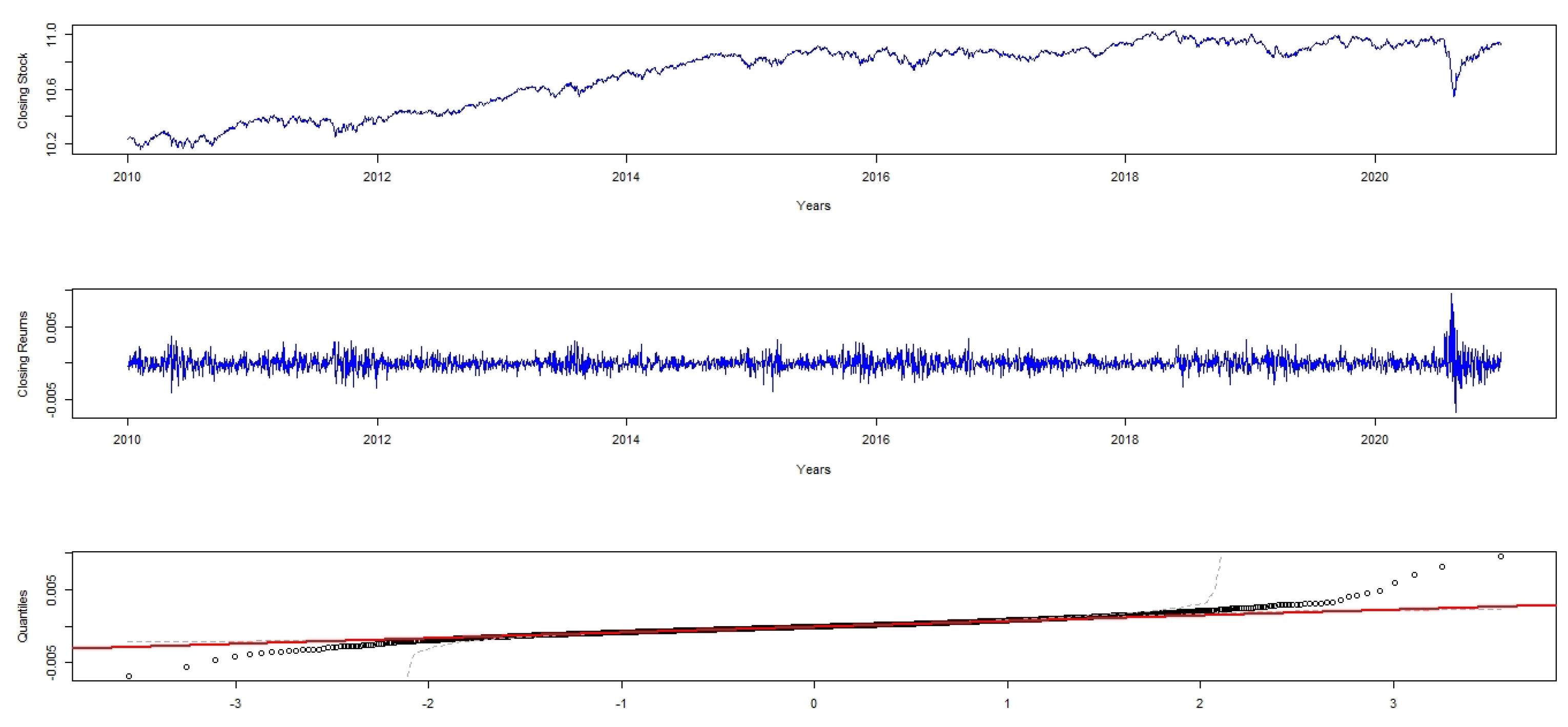
Figure 1 displays intra-day returns on FTSE/JSE-ALSI. The visual inspection of this reveals that the distribution of FTSE/JSE-ALSI is not normally distributed. The quantile-quantile (Q-Q) plot in the last panel reveals a strong departure of linearity in the tails of returns on FTSE/JSE-ALSI. This departure is also evident from

Table 2. Descriptive statistics for intra-day returns with reported skewness and kurtosis of logarithmic returns on FTSE/JSE–ALSI.

	Skewness	Kurtosis
Returns on FTSE/JSE-ALSI	−18.83	688.84

, which gives a descriptive statistics for intra-day returns on FTSE/JSE-ALSI. The reported kurtosis in Table 2 is greater than three and the skewness is less than zero, making the returns to be asymmetric with one heavy, and one semi-heavy tails. Two significant issues are uncovered by these charts; these are the weight easing cause and steady unpredictability. The latter infers that individual shocks often have a long effect on subsequent volatility. The former state that shocks are followed by periods of low volatility rather than high volatility. Similar results were obtained by Musunuru et al. (2013).

3.2. SARIMA–GAS–GEVD Framework

To begin the main analysis, a SARIMA in model (3) is fitted to the training data. This model is used to filter the returns on FTSE/JSE-ALSI in order to obtain independent and identically distributed residuals. Moreover, in order to accommodate the Box-Jenkins methodology, the Augmented Dickey Fuller (ADF) test is applied and the ADF model with intercept and trend is selected because its $Pr\left(t\right)=0.0001$. To test for a long-term trend, a Mann-Kendall test statistics is used and the results of this test statistic revealed a significant monotonic increasing long-term trend in FTSE/JSE-ALSI returns. Finally, ARIMA $(1,0,0)\times {(1,0,0)}_{240}$ is selected as the final model and it is formulated as

$$r_t=\left[\left(1-0.684\mathsf{\Phi }\ast \ast \ast \left(1\right)\right)\times \left(1-0.4532\mathsf{\Phi }\ast \ast \left(240\right)\right)\right]{\epsilon }_t.$$

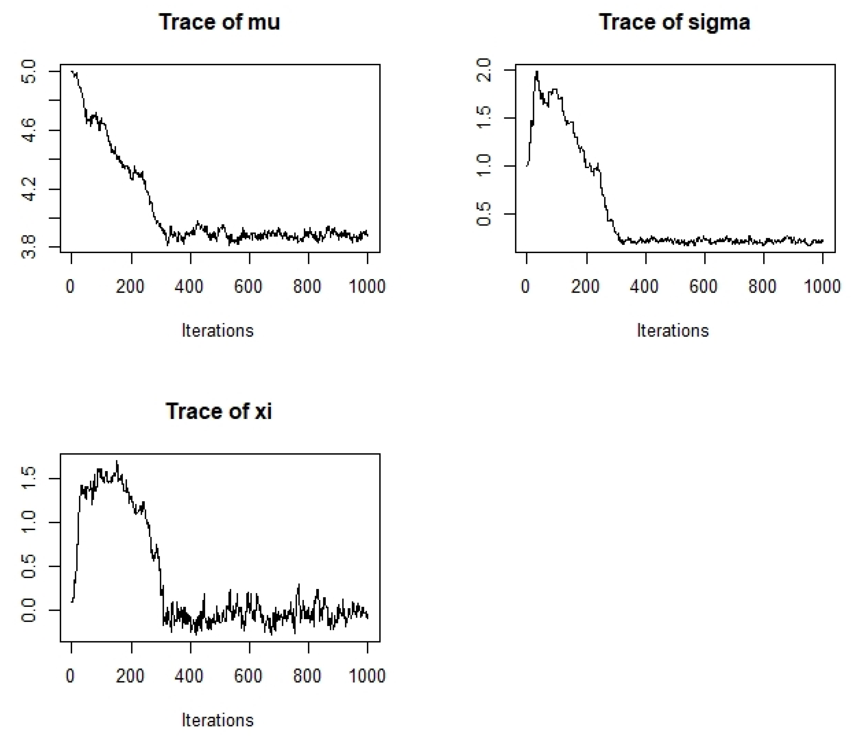
The model diagnosis indicated that the estimated SARIMA model is a white noise process. Using obtained i.i.d residuals and the block size of 2400, the GAS-GEVD is fitted with a total minimas of 482. Estimates of targeted parameters in a skewed student-t distribution are reported in

Table 3. Bayesian parameter estimates of the proposed GAS–GEVD. The estimates are from the i.i.d residuals of the SARIMA model. The GAS–GEVD is fitted using a block minima (BM) with the block size of 2400.

Parameter	Estimate	Std Error	t-Value	$Pr\left(>\mid \mathit{t}\mid \right)$
${\widehat{\varphi }}_1$	65.5515	0.8782	7.4040	0.0000
${\widehat{\varphi }}_2$	0.0702	0.0895	8.7172	0.0000
${\widehat{\varphi }}_3$	3.7575	3.7575	1.4740	0.0702
$\widehat{\sigma }$	9.9995	0.0005	2.0578	0.0000
$\widehat{\xi }$	−1.7119	0.1209	−1.4114	0.0000
$\widehat{\varpi }$	−0.9666	0.0005	−2.0670	0.0000
$\widehat{\mu }$	−0.9356	0.0065	−1.5098	0.0000
Unconditional Parameters
	$\widehat{\mu }$	$\widehat{\sigma }$	$\widehat{\xi }$	$\widehat{\varpi }$
	−0.0046	0.00245	−7.999	1.091

, which reports parameter estimates of the proposed generalized autoregressive-generalized extreme value distribution. Figure 2 shows the traces of $\mu ,\sigma$ and $\xi$, which are produced by running a Markov-chain-Monte-Carlo (MCMC) on the Bayesian estimates of SARIMA $(1,0,0)\times (1,0,0)$. Results in this figure shows those properties that are found in financial econometric literature. These are, but not limited to, strong persistence in volatility and positive reaction of conditional variance to negatively skewed innovations. The choice of a skewed student-t is justified by its significant parameter estimate denoted by $\widehat{\varpi }$. The same results found in this study were also found by Bernardi and Catania (2019) in their study of Switching-GAS copula model for systemic risk assessment. The parameter of excess kurtosis denoted by ${\widehat{\varphi }}_3$ is also significant and it is greater than three. This signifies heavy tails (i.e., leptokurtic) features that have been reported in Table 2. See for instance Gródek-Szostak et al. (2019) and Guégan and Hassani (2019) who also found similar results. In their study on application of the GAS model to stock returns, Makatjane et al. (2017) use the maximum likelihood method to estimate the parameters of the model and these authors also found a leptokurtic behavior in stock returns.

It is worth noting that the fitted skewed student-t distribution follows an extreme distribution that is well known as the Weibull class. This is because the estimated shape parameter denoted as $\widehat{\xi }$ is negative. Gagaza et al. (2019) and Sigauke et al. (2014) also reported a negative shape parameter estimates. The contrast is in an empirical analysis of Chan (2017). These author reported a positive shape parameter in their study, which indicates a Fréchet distribution. Additionally, a 95% confidence interval for the shape parameter is estimated by $\widehat{\xi }\pm z_{\alpha /2}\times \left(se\right)$2 $=-1.7119\pm (1.96\times 0.1209)\approx (-1.948864,-1.474936)$. It can be seen that the interval limits encloses the estimated parameter and therefore conclude that a Weibull is an appropriate distribution for FTSE/JSE-ALSI returns. Finally, the right endpoint is computed as $\widehat{\mu }-\frac{\widehat{\sigma }}{\widehat{\xi }}=4.905570629$ and it implies that for any degree losses above 5%, the likelihood of any further degrease in FTSE/JSE-ALSI is minimal.

3.3. Comparative Analysis

The purpose of this section is to determine the model that best mimics the data and produces less error forecasts. The Akaike information criterion (AIC), Bayesian information criterion (BIC), mean absolute error (MAE), log-likelihood (LL), mean absolute percentage error (MAPE) which are defined in literature as statistical loss function, are used.

Table 4. Shows a comparative analysis of the SARIMA, GAS, GEVD, and the combined SARIMA-GAS-GEVD models to select the best model that mimic the returns on FTSE/JSE-ALSI.

Test	SARIMA	GAS	GEVD	SARIMA-GAS-GEVD
LL	108	110	102	99
Rank	3	4	2	1
AIC	−1710	−1712	−1719	−1725
Rank	4	3	2	1
BIC	−1794	−1799	−1802	−1800
Rank	4	3	1	2
MAE	0.9023	0.988	0.8774	0.9930
Rank	2	3	1	4
MPAE	1.247	1.004	1.002	0.798
Rank	4	3	2	1

shows the statistical loss functions used to compare the estimated models. This helps in selecting the best model that mimic the FTSE/JSE-ALSI returns. Looking at the results of these statistics in Table 4, the log-likelihood and AIC selects a SARIMA–GAS–GEVD as the best performing model. However, the mean absolute error selects the GEVD. Using the rank of 1 to 5, where rank 1 denotes the best model and rank 5 denotes the poorest model, Table 4 gives much evidence that the SARIMA model has the poorest performance because the frequency of rank 4 is higher than the other three models. The final conclusion made here is that SARIMA–GAS–GEVD model outperformed all the models.

3.4. Evaluation of the Prediction Experiment

To reduce variability, a 10-fold cross-validation method is used. This approach partitions the training set into 10 subsets and averages validation results over 10 rounds.

Table 5. Shows the cross-validation performance of the estimated SARIMA–GAS–GEVD on both the training and validation dataset.

Metric	Mean	Std Error	Training Set	Validation Set
Precision	0.9514	0.0108	0.9510	0.9701
Recall	0.9664	0.0107	0.9645	0.9489
F1Score	0.9580	0.0063	0.9577	0.9594
MCC	0.8468	0.0015	0.8489	0.8513
BCR	0.8953	0.0076	0.8909	0.9102

gives the results of cross-validations metrics, which are discussed in Section 2.3. The cross-validations are done on both training and validation data. The SARIMA–GAS–GEVD is evaluated in both training set and validation set, respectively. The classification performance of the model indicates a reasonable goodness-of-fit in the training and validation sets. The average classification on the training set is estimated at 0.9226 while on the validation set it is estimated at 0.92798.

Table 6. Shows a pair-wise comparison and power test to assess the prediction power of SARIMA–GAS–GEVD Model.

	Wilcoxon Signed-Rank Test		Model Power Test
Parameters	SARIMA–GAS–GEVD	Data	Mean Difference	Actual Power
z-value	8.67	Training	−0.0194	0.8241
p-value	0.001	Validation	0.0298	0.8556

shows the pairwise comparison using Wilcoxon signed-rank test and power test using model power prediction. A pair-wise comparison is done to establish the statistical significance of the selected SARIMA–GAS–GEVD model. Chen et al. (2017) and Bui et al. (2016) employed the former, while Karsten et al. (2020) utilized the latter in their empirical analysis in 2020. At 95% confidence level, the null hypothesis is that the model is not statistically different from zero. The relevance of the model is further evaluated by the use of z statistic and p-values. In relation to the actual prediction capacity, the mean difference of the model in both training and validation sets is established and used to complete this assignment. Reject the null hypothesis when z values exceeds the critical value of $(\pm 1.96)$ and when p-values are less than the significant level of $\left(0.05\right)$. The results of a Wilcoxon signed-rank and power tests are shown in Table 6. Since the (p-value = 0.001, z value = 8.67), the model is significantly different from zero, implying a good fit of the SARIMA–GAS–GEVD model. Therefore, this model passes the power test with a score of 82.41%, suggesting that it fits the data well.

3.5. Forecasting and Backtesting Procedure

The forecasting exercise is performed in pseudo real-time and the information that is not accessed is never utilized at the time the forecast is made.

Table 7. Weighted CRPS tests for density forecasts for the extreme time-varying process. The density forecast ˆ ${\widehat{f}}_t+1=N(0,{\widehat{\sigma }}_t^2+1)$ is estimated under the correct model assumption. Its competitor ${\widehat{g}}_t+1=N(0,1{\widehat{\sigma }}_t^2+1)$ uses a deliberately misspecified predictive variance. The width of the sliding training window is $m=76$, and $n=128$ one-step-ahead density forecasts is considered.

Threshold Weights	Emphasis	p-Value	Quantile Weights	p-Value
$W\left(Z\right)={\phi }_{\left\{2.5,1\right\}}\left(Z\right)$	Center	0.1675	$W\left(\alpha \right)=\alpha (1-\alpha )$	0.1892
$W\left(Z\right)=1-{\phi }_{\left\{2.5,1\right\}}\left(Z\right)$	Tails	0.0587	$W\left(\alpha \right)={(2\alpha -1)}^2$	0.0774
$W\left(Z\right)={\theta }_{\left\{2.5,1\right\}}\left(Z\right)$	Left Tail	0.1157	$W\left(\alpha \right)={\alpha }^2$	0.1422
$W\left(Z\right)=1-{\theta }_{\left\{2.5,1\right\}}\left(Z\right)$	Right Tail	0.1005	$W\left(\alpha \right)={(1-\alpha )}^2$	0.9911

shows the comparisons of the threshold and quantile weights forecasting of time-varying VaR and ES. The comparison is based on predicting time-varying VaR and ES at $k=1$ days head, for a test period ranging from the 1 July 2021 to 31 December 2021 for a total $n=128$ density forecast cases. The ES forecast has a clear edge at almost all thresholds and quantiles, with a mean continuous ranked probability score of 0.112%, as opposed to 0.1106% for the VaR forecast. The superiority of ES forecast is corroborated by Table 7, which reports the results of weighted CRPS tests, using the weight functions of Table 1.

Table 8. Backtesting one-step ahead Value-at-Risk and wxpected shortfall at $\alpha =1\%$ risk level using tail risk and dynamic quantile tests. The TR tells how much loss a portfolio can incur while the DQ of the joint hypothesis is at $\alpha$ level of significance.

Risk Measure	TR Test	DQ Test	ADmax	ADMean	AE
VaR	0.4816	7.3246	13.4596	0.5664197	1.1342
ES	0.5364	0.3958	0.48743	0.4873	1.0982

shows results on backtesting one-step ahead density forecasts for VaR and ES. The established tail risk statistic suggest that the null hypothesis is not rejected and conclude that the forecasts of VaR and ES produced reliable, efficient, and unbiased estimates at 1% confidence levels. Under the null hypothesis, there is a correct model specification for the chosen risk level. DQ test statistic p-values for the FTSE/JSE-ALSI returns constituents one-step ahead VaR and ES forecasts at the two downside risk levels $\alpha =1\%$. For long-time periods, the model would produce suitable risk estimates and, according to Bee and Trapin (2018), these long periods are indicated by high probability values of losses at all selected confidence levels for all the tests used. As it is seen in Table 8, none of the tests reject the null hypothesis of vanishing expected score differentials. However, the methods that consider the extreme time-varying volatility show lower violation rates. This is also confirmed by the absolute error loss function.

3.6. Return Level Periods and Bootstrapping Uncertainty Intervals

Table 9. Shows return level periods and posterior distribution with 99% uncertainty interval bootstraps forecasts for VaR and ES.

Period	Returns	Bootstrap Replicates	99% CI
3 Years	4.3760	15,000	(4.2996; 4.3977)
5 Years	5.2416	15,000	(5.166; 5.374)
10 Yeas	6.3842	15,000	(6.287; 6.439)

shows returns level periods and extreme uncertainty interval bootstraps. The bootstrap procedure is developed on the fixed-design residual bootstrap algorithm, which is discussed in Section 2.4. A performance of two distributions as a function of the return period T is explored. It is not phenomenal to calculate return periods as high as 10,000 years relating to a small risk. Ten years, three years and five years, as in Nemukula (2018), are used in the current paper and the results are reported in Table 9. The return levels are obtained by applying a fixed-design residual bootstrap with $B=1500$ replications. As reported in Table 9, a three year return period is 4.376, emphasizing that a daily loss as high as 4.4% would be observed once in three years. The same interpretation can be used for 5-year and 10-year return periods. The estimated bootstrap intervals are not wide, indicating that the MCMC estimates of SARIMA $\left(1,0,0\right)\times {\left(1,0,0\right)}_{240}$–GAS$\left(1\right)$–GEVD are accurate with a forecasting power of 89.6%.

3.7. Discussion of Results

Financial risk is any of the various types of risk associated with financing, including financial transactions of a company loans. Risk analysts can use the proposed loss distributions in this study to predict their financial loss and further estimate the risk associated with their losses. Associated risk factors should be taken into consideration while predicting the loss risk with these loss distributions. Duration of returns on losses could also be increased, as the study used only 3, 5, and 10 year return periods. Insurance companies may also use the estimated time-varying Value-at-Risk and expected shortfall to draw their risk management policy towards their loss on investment and return levels on their losses.

This paper makes use of a stochastic time-varying econometric model and extreme value theory procedures to bootstrap and backtest time varying Value-at-Risk and expected shortfall uncertainty intervals for extreme intra-day return periods. Few studies aim to backtest a one-step-ahead density prediction using time-varying parameters and extreme value distribution. To our knowledge, this is the first use of such a model to produce a map characterizing time-varying and extreme density predictions of VaR ES. To achieve this objective, a three stage procedure is set up. In the first, a SARIMA-GAS-GEVD is estimated and the second stage uncertainty intervals for both ES and the conditional VaR are being bootstrapped by the established fixed-design residual bootstrap procedure. Finally, a 10-fold cross validation and backtesting of the density forecasts that are based on a weighted continuous ranked probability score with the established threshold and quantile weights are used. Robust parameter estimates are achieved by the use of MCMC procedures and setting the number of burns (nburn) and of MCMC replicate to nburn = 1,000,000 L and nmcmc = 810,000 L. This estimation approach produced an overall acceptance sampling rate of 85%, the acceptance rate of the location and a shape parameters at 76.3% and 91.61%, respectively. Estimation of this hybrid has delivered an enhanced understanding for the use of the Bayesian approach to model estimation, bootstrapping, and backtesting time-varying VaR and ES uncertainty intervals for extreme daily return periods. In particular, the study is unique in terms of uniting univariate methods in bootstrapping uncertainty intervals for extreme daily returns. Due to studying a specific sector in the economy, the approach taken in this study best treats the SARMA$(1,0,0){(1,0,0)}_{240}$–GAS(1)–GEVD shape parameter in a simple manner. This has established a significant Weibull distribution in the FTSE/JSE-ALSI returns.

Taking a local density score step as a driving mechanism, time-varying parameters increased and produced a clear indication of a leptokurtic performance in which the empirical properties revealed the same behavior with the volatility of 55.995%. Nevertheless, Anjum and Malik (2020) used a GARCH model with volatility shifts to forecast the conditional VaR. Their approach produced the most accurate VaR forecast relative to several benchmark methods they have used. In this study, the special case of the GARCH model is used, which is the GAS model in collaboration with SARIMA and GEVD. According to Makatjane et al. (2017), the GAS model serves as an extension of the GARCH family models, which assume that the conditional distribution does not vary over time. A vibrant advantage of the GAS model is that it exploits the full likelihood of information. Taking a local density score step as a driving mechanism, the time-varying parameters increase and produced a clear indication of a leptokurtic behavior, in which the empirical properties revealed the same behavior with a skewness of 1.091 in the unconditional parameters. The same behavior of the leptokurtic was also realized in the study of Kamika (2019). When backtesting one-step-ahead density predictions of Value-at-Risk and expected shortfall, no violations were met. All the backtesting tests accepted the null hypothesis, implying that computed risk measures and their uncertainty intervals are reliable and correct future uncertainty signals are given out by these risk measures to the risk managers.

4. Conclusions and Recommendations

The current study aims to empirically investigate the behavior of time-varying uncertainty intervals of ES and VaR by estimating the SARIMA–GAS–GEVD model to the FTSE/JSE-ALSI. The literature on bootstrapping and backtesting uncertainty intervals for extreme return periods while utilizing the SARIMA model combined with GAS–GEVD. No study on the subject are published, and as a result, very few sources are available. The SARIMA(1, 0, 0)(1, 0, 0)–GAS(1)–GEVD is estimated using the Bayesian algorithms in which a non-linear modeling approach with higher dimensions such as GAS-GEVD becomes more complicated, because it has positive semi-definiteness constraints for covariance matrices.

The findings of this study diverge from other previous studies when predicting financial risk. Studies such as Chinhamu et al. (2015) for instance, used only VaR and ES, which is the case in this study. In order to avoid biases that may be caused by using only two risk measures, researchers and scholars should engage more risk measures and avoid using ES and VaR, but use risk measures such as Tail conditional median, expected proportional shortfall, and Wang’s risk measure among others, as these measures and many others are available in the work of Chan and Nadarajah (2019). Additionally, future studies should add one more backtesting procedure known as quantile dynamic test, which was not considered in this study. Moreover, multivariate loss distributions should also be adopted together with multivariate copular methods to test the interdependence and extreme relationships. It would be interesting to see what sort of results would be available when using a machine learning approach to filter the series and quantify one-step-ahead densities for extreme losses and do a comparative analysis with time-varying parameters, extreme value distribution, and bootstrap the credible confidence interval for risk measures. Another area that requires future research is a probabilistic description and modeling of extreme risk loads using the Poison point process. This approach helps in estimating the frequency of the occurrence of peak risks. A sensitivity analysis for daily risk performed and the development of a two-stage stochastic integer recourse models to optimize returns’ distribution is an interesting future research direction.

Banks and stock market participants can use these results to optimist their daily operational one head prediction losses and further predict the probability of future default in their daily operations. Regarding credit risk, the findings can also be useful for banks. Financial risk is any of the various types of risk associated with financing, including financial transactions that include company loans in risk of default. Therefore, risk analysts can use the proposed loss distributions in this study to predict their financial loss and further estimate the risk associated with the losses. Associated risk factors should be taken into consideration while predicting the loss risk with this loss distribution. Duration of returns on losses could also be increased, as the study used only 3-year, 5-year, and 10-year return periods. Insurance companies may also use this model to draw their risk management policy towards their loss on investment and return levels on their losses.

References

- Amisano, Gianni, and Raffaella Giacomini. 2007. Comparing Density Forecasts via Weighted Likelihood Ratio Tests. Journal of Business and Economic Statistics 25: 177–90. [Google Scholar] [CrossRef]
- Anjum, Hassan, and Farooq Malik. 2020. Forecasting Risk in the US Dollar Exchange Rate under Volatility Shifts. The North American Journal of Economics and Finance 54: 101257. [Google Scholar] [CrossRef]
- Ardia, David, Kris Boudt, and Leopoldo Catania. 2019. Generalised Autoregressive Score Models in R: The GAS Package. Journal of Statistical Software 88: 1–28. [Google Scholar] [CrossRef] [Green Version]
- Babatunde, Oluwagbenga Tobi, Henrietta Ebele Oranye, and Cynthia Ndidiamaka Nwafor. 2020. Volatility of Some Selected Currencies Against the Naira Using Generalized Autoregressive Score Models. International Journal of Statistical Distributions and Applications 6: 42–46. [Google Scholar] [CrossRef]
- Bayer, Sebastian, and Timo Dimitriadis. 2020. Regression based expected shortfall backtesting. Journal of Financial Econometrics 18: nbaa013. [Google Scholar] [CrossRef]
- Bee, Marco, and Luca Trapin. 2018. Estimating and Forecasting Conditional Risk Measures with Extreme Value Theory: A Review. Risks 6: 45. [Google Scholar] [CrossRef] [Green Version]
- Bernard, Carole, Ludger Rüschendorf, and Steven Vanduffel. 2017. Value-at-risk Bounds with Variance Constraints. Journal of Risk and Insurance 84: 923–59. [Google Scholar] [CrossRef]
- Bernardi, Mauro, and Leopoldo Catania. 2019. Switching-GAS Copula Models for Systemic Risk Assessment. Journal of Applied Econometrics 34: 43–65. [Google Scholar] [CrossRef] [Green Version]
- Beutner, Eric, Alexander Heinemann, and Stephan Smeekes. 2020. A Residual Bootstrap for Conditional Value-at-Risk. arXiv arXiv:1808.09125. [Google Scholar]
- Bui, Dieu Tien, Tran Anh Tuan, Harald Klempe, Biswajeet Pradhan, and Inge Revhaug. 2016. Spatial Prediction Model for shallow Landslide Hazards: A Comparative Assessment of the Efficacy of Support Vector Machines, Artificial Neural Networks, Kernel Logistic Regression, and Logistic Model Tree. Landslides 13: 361–78. [Google Scholar] [CrossRef]
- Chan, Joshua C. C. 2017. The Stochastic Volatility in Mean Model With Time-Varying Parameters: An Application to Inflation Modeling. Journal of Business and Economic Statistics 35: 17–28. [Google Scholar] [CrossRef]
- Chan, Stephen, and Saralees Nadarajah. 2019. Risk: An R package for Financial Risk Measures. Computational Economics 53: 1337–51. [Google Scholar] [CrossRef] [Green Version]
- Chandiwana, Edina, Caston Sigauke, and Alphonce Bere. 2021. Twenty-Four-Hour Ahead Probabilistic Global Horizontal Irradiance Forecasting Using Gaussian Process Regression. Algorithms 14: 177. [Google Scholar] [CrossRef]
- Chen, Wei, Xiaoshen Xie, Jiale Wang, Biswajeet Pradhan, Haoyuan Hong, Dieu Tien Bui, Zhao Duan, and Jianquan Ma. 2017. A Comparative Study of Logistic Model Tree, Random Forest, and Classification and Regression tree Models for Spatial Prediction of Landslide Susceptibility. Catena 51: 147–60. [Google Scholar] [CrossRef] [Green Version]
- Chinhamu, Knowledge, Chun-Kai Huang, Chun-Sung Huang, and Delson Chikobvu. 2015. Extreme Risk, Value-at-Risk and Expected Shortfall in the Gold Market. The International Business and Economics Research Journal 14: 109–22. [Google Scholar] [CrossRef]
- Christoffersen, Peter F. 1998. Evaluating Interval Forecasts. International Economic Review 39: 841–62. [Google Scholar] [CrossRef]
- Christoffersen, Peter, and Sílvia Gonçalves. 2005. Estimation Risk in Financial Risk Management. The Journal of Risk 7: 1–28. [Google Scholar] [CrossRef] [Green Version]
- Coroneo, Laura, and Fabrizio Iacone. 2020. Comparing Predictive Accuracy in Small Samples using Fixed-smoothing Asymptotics. Journal of Applied Econometrics 35: 391–409. [Google Scholar] [CrossRef]
- Creal, Drew, Siem Jan Koopman, and André Lucas. 2013. Generalized Autoregressive Score Models with Applications. Journal of Applied Econometrics 28: 777–95. [Google Scholar] [CrossRef] [Green Version]
- Droumaguet, Matthieu. 2012. Markov-Switching Vector Autoregressive Models: Monte Carlo Experiment, Impulse Response Analysis, and Granger-Causal. Ph.D. thesis, European University Institute, Europe, Department of Economics, Fiesole, Italy. Available online: http://hdl.handle.net/1814/25135 (accessed on 13 August 2021).
- Eckernkemper, Tobias. 2018. Modelling systemic Risk: Time-varying Tail Dependence when Forecasting Marginal Expected Shortfall. Journal of Financial Economics 16: 63–117. [Google Scholar] [CrossRef]
- Engle, Robert F., and Simone Manganelli. 2004. CAViaR: Conditional Autoregressive Value-at-Risk by Regression Quantiles. Journal of Business and Economic Statistics 22: 412–15. [Google Scholar] [CrossRef]
- Escanciano, J. Carlos, and Jose Olmo. 2010. Backtesting Parametric Value-at-Risk with Estimation Risk. Journal of Business and Economic Statistics 28: 36–51. [Google Scholar] [CrossRef]
- Frésard, Laurent, Christophe Pérignon, and Anders Wilhelmsson. 2011. The Pernicious Effects of Contaminated Data in Risk Management. Journal of Banking and Finance 35: 2569–83. [Google Scholar] [CrossRef]
- Gagaza, Nceba, Murendeni Maurel Nemukula, Retius Chifurira, and Danielle Jade Roberts. 2019. Modelling Non-stationary Temperature Extremes in KwaZulu-Natal using the Generalised Extreme Value Distribution. In Annual Proceedings of the South African Statistical Association Conference. Number Congress 2. Centurion: South African Statistical Association (SASA), pp. 1–8. Available online: https://hdl.handle.net/10520/EJC-19ea5a8642 (accessed on 3 July 2021).
- Gareth, James, Witten Daniela, Hastie Trevor, and Tibshirani Robert. 2013. An Introduction to Statistical Learning with Application in R. New York: Springer, vol. 112, Available online: https://d1wqtxts1xzle7.cloudfront.net/ (accessed on 3 March 2021).
- Ghosh, Bidisha, Biswajit Basu, and Margaret O’Mahony. 2007. Bayesian Time-Series Model for Short-term Traffic Flow Forecasting. Journal of Transportation Engineering 133: 180–89. [Google Scholar] [CrossRef]
- Gneiting, Tilmann, and Roopesh Ranjan. 2012. Comparing Density Forecasts using Threshold-and Quantile-Weighted Scoring Rules. Journal of Business and Economic Statistics 29: 411–22. [Google Scholar] [CrossRef] [Green Version]
- Gródek-Szostak, Zofia, Gabriela Malik, Danuta Kajrunajtys, Anna Szeląg-Sikora, Jakub Sikora, Maciej Kuboń, Marcin Niemiec, and Joanna Kapusta-Duch. 2019. Modelling the Dependency Between Extreme Prices of Selected Agricultural Products on the Derivatives Market using the Linkage Function. Sustainability 11: 4144. [Google Scholar] [CrossRef] [Green Version]
- Guégan, Dominique, and Bertrand K. Hassani. 2019. Risk Measurement: From Quantitative Measures to Management Decisions. Berlin: Springer. [Google Scholar] [CrossRef]
- Hartz, Christoph, Stefan Mittnik, and Marc Paolella. 2006. Accurate Value-at-Risk Forecasting Based on the Normal-GARCH Model. Computational Statistics and Data Analysis 51: 2295–312. [Google Scholar] [CrossRef]
- Harvey, Andrew C. 2013. Dynamic Models for Volatility and Heavy Tails: With Applications to Financial and Economic Time Series. Cambridge: Cambridge University Press, Available online: hppts://www.cambridge.org/9781107630024 (accessed on 27 September 2021).
- Kamika, Mbuaya Grace. 2019. An Application of the Generalised Autoregressive Score Model to Market Risk Modelling. Ph.D. thesis, University of Johannesburg, School of Economics and Econometrics, Johannesburg, South Africa. Available online: http://hdl.handle.net/102000/0002 (accessed on 27 September 2021).
- Karsten, Bettina, Luca Petrigna, Andreas Klose, Antonino Bianco, Nathan Townsend, and Christoph Triska. 2020. Relationship between the critical power test and a 20-min functional threshold power test in cycling. Frontiers in Physiology 11: 613151. [Google Scholar] [CrossRef]
- Kupiec, Paul. 1995. Techniques for Verifying the Accuracy of Risk Measurement Models. The Journal of Derivatives 3: 73–84. Available online: https://ssrn.com/abstract=7065 (accessed on 27 September 2021). [CrossRef]
- Lazar, Emese, and Xiaohan Xue. 2019. Forecasting Risk Measures using Intra-day Data in a Generalized Autoregressive Score Framework. International Journal of Forecasting 36: 1–16. [Google Scholar] [CrossRef]
- Le, Trung H. 2020. Forecasting Value at Risk and Expected Shortfall with Mixed Data Sampling. International Journal of Forecasting 36: 1362–79. [Google Scholar] [CrossRef]
- Makatjane, Katleho, Diteboho Xaba, and Ntebogang Moroke. 2017. Application of Generalized Autoregressive Score Model to Stock Returns. International Journal of Economics and Management Engineering 11: 2714–17. [Google Scholar] [CrossRef]
- Maposa, Daniel. 2016. Statistics of Extremes with Applications to Extreme Flood Heights in the Lower Limpopo River Basin of Mozambique. Ph.D. thesis, University of Limpopo, School of Mathematical and Computer Sciences, Mankweng, South Africa. Available online: http://hdl.handle.net/10386/1695 (accessed on 27 September 2021).
- Maposa, Daniel, Maseka Lesaoana, and James J. Cochran. 2016. Modelling Non-stationary Annual Maximum Flood Heights in the Lower Limpopo River Basin of Mozambique. Jàmbá Journal of Disaster Risk Studies 8: 1–9. [Google Scholar] [CrossRef] [PubMed]
- Masingi, Vusi Ntiyiso, and Daniel Maposa. 2021. Modelling Long-term Monthly Rainfall Variability in Selected Provinces of South Africa: Trend and Extreme Value Analysis Approaches. Hydrology 8: 70. [Google Scholar] [CrossRef]
- Mieth, Robert, Matt Roveto, and Yury Dvorkin. 2002. Risk Trading in a Chance-constrained Stochastic Electricity Market. IEEE Control Systems Letters 5: 199–204. [Google Scholar] [CrossRef]
- Musunuru, Naveen, Mark Yu, and Arley Larson. 2013. Forecasting Volatility of Returns for Corn using GARCH Models. Texas Journal of Agriculture and Natural Resources 26: 42–55. Available online: https://txjanr.agintexas.org/index.php/txjanr/article/view/33/21 (accessed on 27 September 2021).
- Nemukula, Murendeni Maurel. 2018. Modelling Temperature in South Africa using Extreme Value Theory. Ph.D. thesis, University of the Witwatersrand, School of Statistics and Actuarial Science, Johannesburg, South Africa. Available online: https://core.ac.uk/download/pdf/188769682.pdf (accessed on 27 September 2021).
- Nieto, Maria Rosa, and Esther Ruiz. 2016. Frontiers in VaR Forecasting and Backtesting. International Journal of Forecasting 32: 475–50. [Google Scholar] [CrossRef]
- Patton, Andrew J., Johanna F. Ziegel, and Rui Chen. 2019. Dynamic Semi–parametric Models for Expected Shortfall and Value-at-Risk. Journal of Econometrics 211: 388–413. [Google Scholar] [CrossRef] [Green Version]
- Rigotti, Luca, and Chris Shannon. 2005. Uncertainty and Risk in Financial Markets. Econometrica 73: 203–43. [Google Scholar] [CrossRef] [Green Version]
- Rocco, Marco. 2014. Extreme value theory in Finance: A Survey. Journal of Economic Surveys 28: 82–108. [Google Scholar] [CrossRef] [Green Version]
- Siegl, Thomas, and Ansgar West. 2001. Statistical Bootstrapping Methods in VaR Calculation. Applied Mathematical Finance 8: 67–181. [Google Scholar] [CrossRef]
- Sigauke, Caston, Andréhette Verster, and Delson Chikobvu. 2012. Tail Quantile Estimation of Heteroscedastic Intra-day Increases in Peak Electricity Demand. African Review of Economics and Finance 2: 435. [Google Scholar] [CrossRef] [Green Version]
- Sigauke, Caston, Rhoda M. Makhwiting, and Maseka Lesaoana. 2014. Modelling Conditional Heteroscedasticity in JSE Stock Returns using the Generalised Pareto Distribution. African Review of Economics and Finance 6: 41–55. Available online: https://hdl.handle.net/10520/EJC155586 (accessed on 27 September 2021).
- Spierdijk, Laura. 2016. Confidence Intervals for ARMA–GARCH Value-at-risk: The Case of Heavy Tails and skewness. Computational Statistics and Data Analysis 100: 545–59. [Google Scholar] [CrossRef]
- Tafakori, Laleh, Armin Pourkhanali, and Farzad Alavi Fard. 2018. Forecasting Spikes in Electricity Return Innovations. Energy 150: 508–26. [Google Scholar] [CrossRef]
- Taylor, James W. 2019. Forecasting Value–at–Risk and Expected Shortfall using a Semi-parametric Approach Based on the Asymmetric Laplace Distribution. Journal of Business and Economic Statistics 37: 121–33. [Google Scholar] [CrossRef]
- Vidal, Ignacio. 2014. A Bayesian analysis of the Gumbel Distribution: An Application to Extreme Rainfall Data. Stochastic Environmental Research and Risk Assessment 28: 571–82. [Google Scholar] [CrossRef]
- Zoglat, A., S. El Adlouni, E. Ezzahid, A. Amar, C. G. Okou, and F. Badaoui. 2013. Statistical Methods to Expect Extreme Values: Application of Pot Approach to cac40 Return Index. International Journal of Statistics and Economics 10: 1–13. Available online: http://hdl.handle.net/10625/51488 (accessed on 27 September 2021).
Figure 1.
Presents plots of original FTSE/JSE-ALSI, the logarithm returns on FTSE/JSE–ALSI, and normal Q-Q plot for intra-day returns on FTSE/JSE–ALSI.
Figure 2.
Traces of three GEVD for parameters , and showing the maximum iterations used to estimate these parameters.