A Note on Universal Bilinear Portfolios

Abstract

This note provides a neat and enjoyable expansion and application of the magnificent Ordentlich-Cover theory of “universal portfolios”. I generalize Cover’s benchmark of the best constant-rebalanced portfolio (or 1-linear trading strategy) in hindsight by considering the best bilinear trading strategy determined in hindsight for the realized sequence of asset prices. A bilinear trading strategy is a mini two-period active strategy whose final capital growth factor is linear separately in each period’s gross return vector for the asset market. I apply Thomas Cover’s ingenious performance-weighted averaging technique to construct a universal bilinear portfolio that is guaranteed (uniformly for all possible market behavior) to compound its money at the same asymptotic rate as the best bilinear trading strategy in hindsight. Thus, the universal bilinear portfolio asymptotically dominates the original (1-linear) universal portfolio in the same technical sense that Cover’s universal portfolios asymptotically dominate all constant-rebalanced portfolios and all buy-and-hold strategies. In fact, like so many Russian dolls, one can get carried away and use these ideas to construct an endless hierarchy of ever more dominant H-linear universal portfolios.

We first investigate what a natural goal might be for the growth of wealth for arbitrary market sequences. For example, a natural goal might be to outperform the best buy-and-hold strategy, thus beating an investor who is given a look at a newspaper n days in the future. We propose a more ambitious goal.

—Thomas M. Cover, Universal Portfolios, 1991

In 1988, out of the blue, Paul Samuelson wrote a letter to Stanford information theorist Thomas Cover. Samuelson had been sent one of Cover’s papers on portfolio theory for review. “If I did use some of your procedures,” Samuelson wrote, “I would not let that … bias my portfolio choice toward choices my alien cousin with log utility would make”. He chides Kelly, Latané, Markowitz, and “various Ph.D’s who appear with Poisson-distribution probabilities most Junes”.

—William Poundstone, Fortune’s Formula, 2005

With four parameters I can fit an elephant, and with five I can make him wiggle his trunk.

—John von Neumann

1. Introduction; Literature Review

This note contains a nice application and extension of the elegant universal portfolio theory that was established by Thomas Cover (1991); Cover and Ordentlich (1996); and Ordentlich and Cover (1998).

Universal portfolio theory is the on-line analogue of the log-optimal portfolio theory (that is, the theory of asymptotic capital growth), whose brilliant simplicity came down to us from such illustrative thinkers as John Kelly (1956), Henry Latané (1959), Leo Breiman (1961), and card-counter Edward O. Thorp (1969). Under laboratory conditions where the investor or gambler knows in advance the precise distribution of the profit-and-loss outcomes on which he is betting, the tea leaves say (cf. with MacLean et al. (2011)) that log-optimal portfolios (or growth-optimal portfolios) enjoy tremendous optimality properties, quite apart from the fact that they saturate a very specific type of expected utility, as pointed out so many times by Samuelson (1963, 1969, 1979).

Leo Breiman (1961) gave the first substantial results in this direction, namely, that the so-called Kelly gambler will, under general conditions, asymptotically outperform any “essentially different strategy” almost surely by an exponential factor. He also demonstrated that, for the sake of goal-based investing, the Kelly criterion minimizes the expected waiting time with respect to hitting a distant high-water mark.

In a pair of beautiful articles, Bell and Cover(1980, 1988) established that, actually, the Kelly rule also possesses very strong short-term competitive optimality properties, even for a single period’s fluctuation of a betting or investment market. They considered a static, zero-sum investment ϕ-game whose payoff kernel is equal to the expected value of an arbitrary increasing function $\varphi (•)$ of the ratio of one trader’s wealth to that of another. Subject to the proviso that, prior to the actual portfolio choice, each contestant is permitted to make a fair randomization of his initial dollar (by exchanging it for any random capital whose mean is at most 1), the saddle point of the game amounts to each player using the log-optimal portfolio, together with fair randomizations that depend only on the criterion $\varphi (•)$, and not on any particular characteristic of the underlying investment opportunities.

Garivaltis (2018a) showed that the Bell-Cover theorem holds equally well for stochastic differential investment $\varphi$-games in continuous time that exhibit state-dependent drift and diffusion; Garivaltis (2019a) generalized this result even further, so as to cover levered investment $\varphi$-games over continuous time markets whereby the asset prices follow jump-diffusion processes with compactly-supported jump returns. Some recent work by Curatola (2019) investigates the strategic interaction of two large traders whose transactions affect not just each other, but also the expected returns of the entire stock market. For an illuminating discussion of competitive optimality as it relates to evolutionary contingencies in mathematical biology, consult with Tal and Tran (2020).

Cover’s universal portfolio theory, which began in earnest with his empirical Bayes stock portfolio (Cover and Gluss (1986)), takes its cue from the fact that for stock markets with iid returns, the log-optimal portfolio amounts to a certain constant-rebalanced portfolio (CRP); this consists in fixing the correct (growth-optimal) target percentages of wealth for each asset, and continuously executing rebalancing trades so as to counteract allocation drift. However, in the presence of model uncertainty (e.g., for actual stock markets), this particular CRP is completely unknown to the practitioner.

Inspired by the analogies with information theory, Thomas Cover had the brilliant insight that one should benchmark his on-line investment performance relative to that of the best constant-rebalanced portfolio determined in hindsight for the actual (realized) sequence of asset prices. The hindsight-optimized wealth can be interpreted as a financial derivative that is susceptible of exact pricing and replication in the (complete) continuous time market of Black and Scholes (1973). On that score, Ordentlich and Cover (1998) priced the rebalancing option at time-0 for unlevered hindsight optimization over a single risk asset; their work sat unfinished for twenty years, until it was completed by Garivaltis (2019b), who demonstrated how to price and replicate Cover’s (levered) rebalancing option at any time t, for any number of correlated stocks in geometric Brownian motion.

In discrete time, the empirical Bayes stock portfolio (Cover and Gluss (1986)), the Dirichlet-weighted universal portfolio (Cover and Ordentlich (1996)), and the minimax universal portfolio (Ordentlich and Cover (1998)) are all notable in that they guarantee to achieve a high percentage of the final wealth of the best constant-rebalanced portfolio in hindsight, uniformly for all possible sequences of asset prices. On account of the fact that this percentage (or competitive ratio) converges to zero at a slow (polynomial) rate, the excess compound (logarithmic) growth rate of the best CRP in hindsight (over and above that of the on-line portfolio) converges uniformly to zero. Thus, universal portfolios succeed in matching the performance of the best CRP in hindsight “to first order in the exponent”.

The original universal portfolios (inspired as they were by iid stock markets) suffer from the defect that they fail to recognize and exploit even very simple types of serial dependence in the individual sequence of asset returns. For example, consider a two-asset market whereby asset 2 is cash (that pays no interest), and asset 1 is a “hot stock” whose price alternately doubles in odd periods and gets cut in half in even periods. Naturally, one should hope that his portfolio selection algorithm is capable of detecting such a trivial pattern, thereby learning to (asymptotically) double its capital every two periods. But the original universal portfolios, when applied to this particular sequence of asset prices, merely learn to use the constant-rebalanced portfolio that puts $50\%$ of its wealth into the stock and holds the rest in cash at the start of each investment period; this generates asymptotic capital growth at a rate of $\log (9/8)=11.8\%$ every two periods, compounded continuously—a far cry from the $\log 2=69.3\%$ that accrues to perfect trading.

One way out of this conundrum is the use the universal portfolio with side information (Cover and Ordentlich (1996)) along with a “signal” that indicates, say, whether or not the current period is odd. The obvious objection here is that the efficacy of this particular signal (as opposed to any other piece of side information) will only ever become apparent in hindsight. Accordingly, this paper tackles the problem differently: we consider an expanded parametric family of mini 2-period active trading strategies called bilinear portfolios, which explicitly generalize the constant-rebalanced portfolios (here called 1-linear portfolios). Accordingly, we apply the Ordentlich-Cover techniques to design a universal bilinear portfolio that compounds its money at the same asymptotic rate as the best bilinear trading strategy in hindsight (thereby learning to trade perfectly in the motivating example). Thus, the universal bilinear portfolio will be shown to asymptotically dominate the universal 1-linear portfolio in the same technical sense (cf. with Cover and Thomas (2006)) that the universal 1-linear portfolio asymptotically dominates all constant-rebalanced portfolios and all buy-and-hold strategies. Once this is done, it will become readily apparent just how one can go about constructing an endless hierarchy of ever more dominant universal H-linear portfolios, for all possible mini-horizons $H\in \left\{1,2,3,...\right\}$.

2. Bilinear Trading Strategies

We start by defining the concept of a bilinear trading strategy (or bilinear portfolio), which is a simple 2-period active strategy that generalizes the notion of a constant-rebalanced portfolio (CRP). To this end, we assume that there are m assets called $i,j\in \{1,...,m\}$; we let $x_i\ge 0$ denote the gross return1 of a $\$1$ investment in asset i in period 1, and similarly we let $y_j\ge 0$ denote the gross return of asset j in period 2. We let $x:={(x_1,...,x_m)}^{\prime }\in {\mathbb{R}}_{+}^m-\left\{0\right\}$ denote the gross return vector in period 1, and in the same vein, $y:={(y_1,...,y_m)}^{\prime }\in {\mathbb{R}}_{+}^m-\left\{0\right\}$ is the gross return vector in period 2.

Definition 1.

A bilinear trading strategy is a square matrix $B:={\left[b_{ij}\right]}_{m\times m}$ of non-negative weights that sum to one. After two investment periods, the bilinear trading strategy B multiplies the initial dollar by a factor of

$$\begin{array}{|c|}\hline \mathrm{TWO}\text{-}\mathrm{PERIOD}\mathrm{CAPITAL}\mathrm{GROWTH}\mathrm{FACTOR}:=x^{\prime }By={\displaystyle \sum _{i=1}^m}{\displaystyle \sum _{j=1}^m}{b}_{ij}{x}_i{y}_j.\\ \hline\end{array}$$

(1)

The set of all bilinear trading strategies is denoted

$$\mathcal{B}:=\left\{B\in {\mathit{Mat}}_{m,m}\left(\mathbb{R}\right):B\ge 0\mathit{and}{\mathbf{1}}^{\prime }B\mathbf{1}=1\right\},$$

(2)

where $\mathbf{1}:={(1,...,1)}^{\prime }$ is an $m\times 1$ vector of ones.

Proposition 1.

The bilinear2 final wealth $x^{\prime }By$ is uniquely replicated by the following 2-period active trading strategy: in period 1, we use the initial portfolio $p:={(p_1,...,p_m)}^{\prime }=B\mathbf{1}$, where $p_i={\displaystyle \sum _{j=1}^m}{b}_{ij}$ is the initial fraction of wealth that will be invested in asset i; in period 2, we must use the portfolio

$$\begin{array}{|c|}\hline q\left(x\right):={\left(q_1\left(x\right),...,q_m\left(x\right)\right)}^{\prime }=\frac{B^{\prime }x}{p^{\prime }x}=\frac{B^{\prime }x}{x^{\prime }B\mathbf{1}},\\ \hline\end{array}$$

(3)

e.g.,

$$q_j\left(x\right)=\frac{{\displaystyle \sum _{i=1}^m}{b}_{ij}{x}_i}{{\displaystyle \sum _{i=1}^m}{\displaystyle \sum _{k=1}^m}{b}_{ik}{x}_i}.$$

(4)

Proof. 

We start with the functional equation

$$\left(p^{\prime }x\right)·\left(q{\left(x\right)}^{\prime }y\right)=x^{\prime }By,$$

(5)

e.g., the two-period growth factor is equal to the product of the individual growth factors that were achieved in periods 1 and 2. To start, we substitute $y:=\mathbf{1}={(1,...,1)}^{\prime }$ and $x:=e_i={(0,...,0,\underset{i}{1},0,...,0)}^{\prime },$ which is the $i\mathrm{th}$ unit basis vector for ${\mathbb{R}}^m$. There lies $p_i=e_i^{\prime }B\mathbf{1}={\displaystyle \sum _{j=1}^m}{b}_{ij}$, as promised. Next, in the identity

$$q{\left(x\right)}^{\prime }y=\frac{x^{\prime }By}{p^{\prime }x},$$

(6)

we put $y:=e_j$. This leaves us with

$$q_j\left(x\right)=\frac{{\displaystyle \sum _{i=1}^m}{b}_{ij}{x}_i}{{\displaystyle \sum _{i=1}^m}{\displaystyle \sum _{j=1}^m}{b}_{ik}{x}_i},$$

(7)

which is the desired result. In order to be logically complete, we must substitute our expressions for p and $q\left(x\right)$ into Equation (5) so as to verify that they turn it into an identity. Here you go:

$${\left(B\mathbf{1}\right)}^{\prime }x·{\left(\frac{B^{\prime }x}{x^{\prime }B\mathbf{1}}\right)}^{\prime }y=x^{\prime }By.$$

(8)

 □

Example 1.

Every constant-rebalanced portfolio (cf. with Thomas Cover (1991)) $c:={(c_1,...,c_m)}^{\prime }$ amounts to a bilinear trading strategy that is represented by the outer product $B:=c{c}^{\prime }$, e.g., $b_{ij}:=c_i{c}_j$ for all $i,j\in \left\{1,...,m\right\}$. Here, the constant-rebalanced portfolio c resolves to maintain the constant fraction $c_i$ of wealth in each asset i at all times3, where $c_i\ge 0$ and ${\displaystyle \sum _{i=1}^m}{c}_i=1$.

Example 2.

More generally, consider the trading strategy that always uses the portfolio $c:={(c_1,...,c_m)}^{\prime }\in {\Delta }_m$ in period 1 and then always uses the portfolio $d:={(d_1,...,d_m)}^{\prime }\in {\Delta }_m$ in period 2 (regardless of the observed value of x), where ${\Delta }_m:=\left\{c\in {\mathbb{R}}_{+}^m:{\displaystyle \sum _{i=1}^m}{c}_i=1\right\}$ denotes the unit portfolio simplex in ${\mathbb{R}}_{+}^m$. This scheme is a bilinear trading strategy that corresponds to the outer product $B:=c{d}^{\prime }$, e.g., $b_{ij}:=c_i{d}_j$ for all $i,j\in \left\{1,...,m\right\}$.

Example 3.

Every buy-and-hold strategy (that buys some initial portfolio $c:={(c_1,...,c_m)}^{\prime }$ and holds it for two periods, without rebalancing) amounts to a bilinear trading strategy that is represented by the diagonal matrix $B:=\mathrm{diag}(c_1,...,c_m)$.

Inspired by Ordentlich and Cover (1998) and Cover and Thomas (2006), we note that the concept of a bilinear trading strategy admits the following simple and lucid interpretation. Let an extremal strategy4 be defined by the simple trading scheme: in period 1, we put $100\%$ of wealth into asset i, and then in period 2, we take all the proceeds and roll them over into asset j. Hence, there are $m^2$ different extremal strategies $(i,j)\in \{1,...,m\}\times \{1,...,m\}$; since the ${(i,j)}^{th}$ extremal strategy yields a capital growth factor of $x_i{y}_j$, it therefore amounts to the bilinear trading strategy $B:=e_i{e}_j^{\prime }$, which is an extreme point of $\mathcal{B}$. The general bilinear portfolio $B:={\left[b_{ij}\right]}_{m\times m}$ is uniquely representable as a convex combination

$$B={\displaystyle \sum _{i=1}^m}{\displaystyle \sum _{j=1}^m}{b}_{ij}{e}_i{e}_j^{\prime }$$

(9)

of extremal strategies; this means that the practitioner of B has elected to invest the fraction $b_{ij}$ of his initial dollar into each extremal strategy $(i,j)$. Thus, after the elapse of two periods, the investor’s total wealth will be equal to ${\displaystyle \sum _{i=1}^m}{\displaystyle \sum _{j=1}^m}{b}_{ij}{x}_i{y}_j=x^{\prime }By.$

3. Universal Bilinear Portfolios

We now consider the on-line learning of the asymptotically dominant (or growth-optimal) bilinear portfolio. To this end, we assume that there are T basic investment periods $t\in \left\{1,...,T\right\}$, each of which is divided into a “first half” (during which the gross return vector is $x_t$) and a “second half” (during which the gross return vector is $y_t$.) We let $x^t:=(x_1,...,x_t)\in {\left({\mathbb{R}}_{+}^m-\left\{0\right\}\right)}^t$ denote the history of returns in the first halves of periods $1,...,t$, and, likewise, we let $y^t:=(y_1,...,y_t)\in {\left({\mathbb{R}}_{+}^m-\left\{0\right\}\right)}^t$ denote the return history for the latter halves of periods $1,...,t$. Thus, we have the transition laws $x^{t+1}:=(x^t,x_{t+1})$ and $y^{t+1}:=(y^t,y_{t+1})$, where $x^0$ and $y^0$ denote empty histories. We let

$$\begin{array}{|c|}\hline W_B(x^t,y^t):={\displaystyle \prod _{s=1}^t}{x}_s^{\prime }B{y}_s\\ \hline\end{array}$$

(10)

denote the final wealth function5 of the bilinear trading strategy B against the return history $(x^t,y^t)$; similarly, we write

$$W_B(x^t,y^{t-1}):=\left({\displaystyle \prod _{s=1}^{t-1}}{x}_s^{\prime }B{y}_s\right)\times \left(x_t^{\prime }B\mathbf{1}\right)=W_B\left(x^t,(y^{t-1},\mathbf{1})\right)$$

(11)

if period t has only been half-completed. We will consider sequential investment strategies $\widehat{B}(•,•)$ that, at the start of each period t, select some bilinear portfolio $\widehat{B}\left(x^{t-1},y^{t-1}\right):={\left[{\widehat{b}}_{ij}\left(x^{t-1},y^{t-1}\right)\right]}_{m\times m}$ that is conditioned on the observed return history $(x^{t-1},y^{t-1})$; this bilinear portfolio will be used for the entire duration of period t. The capital growth factor achieved by an investment scheme $\widehat{B}(•,•)$ against the history $(x^t,y^t)$ is equal to

$$\widehat{W}(x^t,y^t):={\displaystyle \prod _{s=1}^t}{x}_s^{\prime }\widehat{B}(x^{s-1},y^{s-1})y_s,$$

(12)

and, if period t is only half-finished, we write

$$\widehat{W}(x^t,y^{t-1}):=\left[{\displaystyle \prod _{s=1}^{t-1}}{x}_s^{\prime }\widehat{B}(x^{s-1},y^{s-1})y_s\right]\times \left[x_t^{\prime }\widehat{B}(x^{t-1},y^{t-1})\mathbf{1}\right]=\widehat{W}\left(x^t,(y^{t-1},\mathbf{1})\right).$$

(13)

Within a given period t, the on-line behavior of $\widehat{B}(•,•)$ amounts to the portfolio vectors $\widehat{p}(x^{t-1},y^{t-1}):=\widehat{B}(x^{t-1},y^{t-1})\mathbf{1}$ and

$$\widehat{q}(x^t,y^{t-1}):=\frac{\widehat{B}{(x^{t-1},y^{t-1})}^{\prime }{x}_t}{x_t^{\prime }\widehat{B}(x^{t-1},y^{t-1})\mathbf{1}}.$$

(14)

In order to have a practical benchmark for the on-line performance of $\widehat{B}(•,•)$ after the elapse of t complete investment periods, we will consider the best bilinear trading strategy in hindsight for the individual sequence $(x^t,y^t)$:

$$\begin{array}{|c|}\hline B^{*}(x^t,y^t):=\underset{B\in \mathcal{B}}{\arg \max } W_B(x^t,y^t)\\ \hline\end{array}$$

(15)

and

$$B^{*}(x^t,y^{t-1}):=\underset{B\in \mathcal{B}}{\arg \max } W_B(x^t,y^{t-1})=B^{*}\left(x^t,(y^{t-1},\mathbf{1})\right).$$

(16)

The final wealth that accrues to $B^{*}(x^t,y^t)$ is a path-dependent financial derivative, with payoff

$$\begin{array}{|c|}\hline D(x^t,y^t):=\underset{B\in \mathcal{B}}{\max }{W}_B(x^t,y^t)=W_{B^{*}(x^t,y^t)}(x^t,y^t)\\ \hline\end{array}$$

(17)

and

$$D(x^t,y^{t-1}):=\underset{B\in \mathcal{B}}{\max } W_B(x^t,y^{t-1})=D\left(x^t,(y^{t-1},\mathbf{1})\right).$$

(18)

Proposition 2.

The final wealth function $W_B(x^T,y^T)$ is a multilinear form in the vectors $x_1,y_1,$$x_2,y_2,...,x_T,y_T$, e.g., it is linear separately in each vector $x_t$ and also in each vector $y_t$, for $1\le t\le T.$ Consequently, the hindsight-optimized final wealth $D(x^T,y^T)$ is convex and positively homogeneous separately in each $x_t$ and also in each $y_t$.

Proof. 

The multi-linearity of $W_B(•,•)$ follows easily from the definition, e.g., $W_B(x^T,y^T)=\left({\displaystyle \prod _{s=1}^{t-1}}{x}_s^{\prime }B{y}_s\right)·\left(x_t^{\prime }B{y}_t\right)·\left({\displaystyle \prod _{s=t+1}^T}{x}_s^{\prime }B{y}_s\right)$ is clearly additive and homogeneous in $x_t$ and also in $y_t$. If we write $D\left(x_t\right)$ and view $D(•,•)$ as a function of $x_t$ alone, then the convexity and homogeneity with respect to $x_t$ (or with respect to $y_t$) follow from the fact that the mapping $x_t\mapsto D\left(x_t\right)$ is a pointwise maximum of a family of linear functions, namely, ${\left(W_B\left(x_t\right)\right)}_{B\in \mathcal{B}}$. □

For obvious reasons, the hindsight-optimized payoff $D(•,•)$ is not achievable by any causal (or non-anticipating) investment strategy $\widehat{B}(•,•)$; however, it is possible to achieve6 any average

$$\widehat{W}(x^t,y^t):=\underset{B\in \mathcal{B}}{\int }{W}_B(x^t,y^t)f\left(B\right)dB,$$

(19)

where $f(•)$ is a continuous density function over $\mathcal{B}$. That is, inspired by Thomas Cover (1991) and Cover and Ordentlich (1996), we make the following definition.

Definition 2.

Theuniversal bilinear portfolio(that corresponds to the prior density $f(•)$) is a performance-weighted average of all bilinear-trading strategies:

$$\begin{array}{|c|}\hline \widehat{B}(x^t,y^t):=\frac{\underset{B\in \mathcal{B}}{\int }B·W_B(x^t,y^t)f\left(B\right)dB}{\underset{B\in \mathcal{B}}{\int }{W}_B(x^t,y^t)f\left(B\right)dB}=\frac{{\mathbb{E}}_f\left[B·W_B(x^t,y^t)\right]}{{\mathbb{E}}_f\left[W_B(x^t,y^t)\right]}.\\ \hline\end{array}$$

(20)

So-defined, the matrix $\widehat{B}(•,•)$ is indeed a valid bilinear portfolio, on account of the fact that $\widehat{B}(x^t,y^t)\ge 0$ and ${\mathbf{1}}^{\prime }\widehat{B}(x^t,y^t)\mathbf{1}=1$. The initial bilinear portfolio $\widehat{B}(x^0,y^0)$ is equal to the center of mass $\underset{B\in \mathcal{B}}{\int }Bf\left(B\right)dB={\mathbb{E}}_f\left[B\right]$ that is induced by the prior density $f(•)$.

Proposition 3.

After T complete investment periods, the universal wealth $\widehat{W}(x^T,y^T)$ is equal to the average value

$$\begin{array}{|c|}\hline \widehat{W}(x^T,y^T)=\underset{B\in \mathcal{B}}{\int }{W}_B(x^T,y^T)f\left(B\right)dB={\mathbb{E}}_f\left[W_B(x^T,y^T)\right].\\ \hline\end{array}$$

(21)

Proof. 

The gross return of the universal bilinear portfolio in period t is given by

$$\begin{array}{cc}{x}_t^{\prime }\widehat{B}(x^{t-1},y^{t-1})y_t\hfill & =\frac{\underset{B\in \mathcal{B}}{\int }\left(x_t^{\prime }B{y}_t\right)·W_B(x^{t-1},y^{t-1})f\left(B\right)dB}{\underset{B\in \mathcal{B}}{\int }{W}_B(x^{t-1},y^{t-1})f\left(B\right)dB}\\ \hfill & =\frac{\underset{B\in \mathcal{B}}{\int }{W}_B(x^t,y^t)f\left(B\right)dB}{\underset{B\in \mathcal{B}}{\int }{W}_B(x^{t-1},y^{t-1})f\left(B\right)dB}.\hfill \end{array}$$

(22)

Taking the (telescopic) product of both sides of Equation (22) for $t:=1,...,T$, and bearing in mind that $W_B(x^0,y^0)=1=\underset{B\in \mathcal{B}}{\int }f\left(B\right)dB$, we arrive at the desired result: $\widehat{W}(x^T,y^T)=\underset{B\in \mathcal{B}}{\int }{W}_B(x^T,y^T)f\left(B\right)dB$. □

Following Cover (1991) and Cover and Thomas (2006), the intuition behind the universal bilinear portfolio is just this: we distribute the initial dollar (according to $f(•)$) among all the bilinear trading strategies $B\in \mathcal{B}$, whereby the bilinear portfolios in the neighborhood of a given B receive $f\left(B\right)dB$ dollars to manage (from now until kingdom come). After the elapse of t complete investment periods, the bilinear strategies in this locale have grown their bankroll to $W_B(x^t,y^t)f\left(B\right)dB$; the investor’s aggregate wealth is thereby equal to $\underset{B\in \mathcal{B}}{\int }{W}_B(x^t,y^t)f\left(B\right)dB.$ With this intuition in hand, the formula for $\widehat{B}(x^t,y^t)$ can be written down immediately, on account of the fact that the locale of a given B is responsible for managing the fraction $\varphi \left(B\right)dB:=W_B(x^t,y^t)f\left(B\right)dB/\underset{B\in \mathcal{B}}{\int }{W}_B(x^t,y^t)f\left(B\right)dB$ of the aggregate wealth.

Hence, the overall bilinear portfolio is just the convex combination $\widehat{B}=\underset{B\in \mathcal{B}}{\int }B·\varphi \left(B\right)dB$. Over long periods of time, the bilinear trading strategies in the neighborhood of $B^{*}(x^t,y^t)$ will come to control an ever-greater share of the aggregate wealth, on account of their superior exponential growth rate, namely $(1/t)\log D(x^t,y^t)$. Thus, the aggregate bankroll will (asymptotically) compound itself at this same rate; that is, we have the relation

$$\begin{array}{c}\underset{t\to \infty }{\lim }\left(\mathrm{Excess}\mathrm{Growth}\mathrm{Rate}\mathrm{of}\mathrm{the}\mathrm{Best}\mathrm{Bilinear}\mathrm{Portfolio}\mathrm{in}\mathrm{Hindsight}\right)\hfill \\ \hfill =\underset{t\to \infty }{\lim }\left[\frac{\log D(x^t,y^t)}{t}-\frac{\log \widehat{W}(x^t,y^t)}{t}\right]=0,\end{array}$$

(23)

regardless7 of the individual return sequence $\omega :={(x_t,y_t)}_{t=1}^{\infty }$. The remainder of the paper is concerned with fleshing out the necessary details. On that score, we make the definition:

Definition 3.

The competitive ratio $R(x^T,y^T)$ measures the percentage of hindsight-optimized bilinear wealth that was actually achieved by the universal bilinear portfolio, e.g.,

$$R(x^T,y^T):=\frac{\widehat{W}(x^T,y^T)}{D(x^T,y^T)}=\frac{\mathrm{AVERAGE}\mathrm{VALUE}\mathrm{OF}{W}_B(x^T,y^T)}{\mathrm{MAXIMUM}\mathrm{VALUE}\mathrm{OF}{W}_B(x^T,y^T)}.$$

(24)

Lemma 1.

The competitive ratio $R(•,•)$ is always $\le 1$; it is homogeneous of degree 0 and quasi-concave separately in each vector $x_t$ and also in each vector $y_t$.

Proof. 

The fact that $R(x^T,y^T)\le 1$ follows immediately from the fact that any convex combination (or weighted average) of the numbers ${\left(W_B(x^T,y^T)\right)}_{B\in \mathcal{B}}$ cannot exceed their maximum. The homogeneity of degree 0 follows from the fact that $W_B(•,•)$ and $D(•,•)$ are both linearly homogeneous (of degree 1) in each vector $x_t$ or $y_t$. The multi-quasi-concavity obtains from the fact that, when viewed as a function $R\left(x_t\right)$ of $x_t$ alone (or of $y_t$ alone), we are dealing with the ratio of a positive linear function (namely, $\widehat{W}\left(x_t\right)$) to a positive convex function (viz., $D\left(x_t\right)$). That is, if we consider the upper contour sets

$$U_{\alpha }:=\left\{x_t\in {\mathbb{R}}_{+}^m:R\left(x_t\right)\ge \alpha \right\}=\left\{x_t\in {\mathbb{R}}_{+}^m:\widehat{W}\left(x_t\right)-\alpha D\left(x_t\right)\ge 0\right\},$$

(25)

then we see that $U_{\alpha }$ is a convex set for all $\alpha \in \mathbb{R}$. For, if $\alpha \le 0$, then $U_{\alpha }={\mathbb{R}}_{+}^m$, which is convex; if $\alpha \ge 0$, then $U_{\alpha }$ is convex because it is an upper contour set of the concave function $x_t\mapsto \widehat{W}\left(x_t\right)-\alpha D\left(x_t\right)$. □

On account of the (multi-) homogeneity of degree 0, the competitive ratio only cares about the directions of the vectors $x_t$ or $y_t$—their lengths do not affect the relative performance of the universal bilinear portfolio. Thus, we are free to scale each $x_t$ (resp. $y_t$) by a factor of $\lambda :=1/\left|\right|x_t{\left|\right|}_1$ (resp. $1/\left|\right|y_t{\left|\right|}_1$), so that the coordinates of $x_t$ (resp. $y_t$) sum to one, e.g., we may assume that each $x_t$ or $y_t$ belongs to the unit simplex ${\Delta }_m$. Hence, we have the relation

$$\underline{R}(x^T,y^T):=\underset{(x^T,y^T)\in {\left({\mathbb{R}}_{+}^m-\left\{0\right\}\right)}^{2T}}{\inf }R(x^T,y^T)=\underset{(x^T,y^T)\in {\Delta }_m^{2T}}{\min }R(x^T,y^T),$$

(26)

e.g., the worst-case8 relative performance $\underline{R}(x^T,y^T)$ is achieved over the product of simplices ${\Delta }_m^{2T}$. Even better, since $R(•,•)$ is multi-quasi-concave, its minimum value must in fact be realized at some extreme point $(x^T,y^T)\in {\{e_1,...,e_m\}}^{2T}$, e.g., a return history whereby all $x_t,y_t$ are unit basis vectors. This happens on account of the fact that when $R(•,•)$ is viewed as a function solely of $x_t\in {\Delta }_m$ (or solely of $y_t\in {\Delta }_m$), we have

$$R\left(x_t\right)=R(x_{t1}{e}_1+···+x_{tm}{e}_m)\ge \min \left\{R\left(e_1\right),...,R\left(e_m\right)\right\}=R\left(e_{i^{*}}\right),$$

(27)

so that the competitive ratio can always be reduced by replacing any $x_t$ or $y_t$ by an appropriate unit basis vector $e_{i^{*}}$.

In what follows, we will consider sequences of unit basis vectors $x^T:=(e_{i_1},...,e_{i_T})$ and $y^T:=(e_{j_1},...,e_{j_T})$, where $i^T:=(i_1,...,i_T)\in {\{1,...,m\}}^T$ and $j^T:=(j_1,...,j_T)\in {\{1,...,m\}}^T$. For the sake of simplicity, we will abuse notation by writing the (self-evident) expressions $R(i^T,j^T)$, $\widehat{W}(i^T,j^T)$, and $D(i^T,j^T)$. Sequences of unit basis vectors will hereby be referred to as extremal sequences, or Kelly horse race sequences, on account of the fact that they correspond to betting markets (say, horse races or prediction markets) whereby only one of the m assets has a positive gross return. For a given Kelly sequence $(i^T,j^T)$, we will require the counts, or relative frequencies

$$n_{ij}(i^T,j^T): :=: \left(\mathrm{number}\mathrm{of}\mathrm{times}(i_t,j_t)=(i,j)\right)=\sum _{\left\{t:(i_t,j_t)=(i,j)\right\}}1,$$

(28)

so that $n_{ij}\ge 0$ and ${\displaystyle \sum _{i=1}^m}{\displaystyle \sum _{j=1}^m}{n}_{ij}=T$.

Lemma 2.

For any Kelly sequence $(i^T,j^T)$, the final wealth of the best bilinear trading strategy in hindsight is equal to $D\left({\left[n_{ij}\right]}_{i,j=1}^m\right)={\displaystyle \prod _{(i,j):n_{ij}>0}}{(n_{ij}/T)}^{n_{ij}}$; the universal wealth $\widehat{W}(i^T,j^T)$ admits the minorant

$$\widehat{W}(i^T,j^T)\ge \frac{\underline{f}}{(T+m^2-1)!}{\displaystyle \prod _{i=1}^m}{\displaystyle \prod _{j=1}^m}{n}_{ij}!,$$

(29)

where $\underline{f}:=\underset{B\in \mathcal{B}}{\min }f\left(B\right)$ is the minimum weight assigned to any bilinear portfolio by the prior density $f(•)$.

Proof. 

Against the Kelly sequence $(i^T,j^T)$, the final wealth of the bilinear trading strategy B is given by

$$W_B(i^T,j^T)={\displaystyle \prod _{t=1}^T}{b}_{i_t{j}_t}=\prod _{(i,j):n_{ij}>0}{b}_{ij}^{n_{ij}(i^T,j^T)}.$$

(30)

Maximization of this quantity with respect to B amounts to a standard Cobb-Douglas optimization problem over the unit simplex in ${\mathbb{R}}_{+}^{m^2}$. Lagrange’s multipliers yield the solution $b_{ij}^{*}=n_{ij}/T$, so that $D(i^T,j^T)={\displaystyle \prod _{(i,j):n_{ij}>0}}{(n_{ij}/T)}^{n_{ij}}$.

The stated minorant for $\widehat{W}(i^T,j^T)$ will be gotten by direct integration of $W_B(i^T,j^T)$ over the set of bilinear trading strategies. To this end, we will identify $\mathcal{B}$ with the solid region

$$\left\{\left(b_{11},...,b_{1m},b_{21},...,b_{2m},...,b_{m1},...,b_{m,m-1}\right)\in {\mathbb{R}}_{+}^{m^2-1}:b_{11}+···+b_{m,m-1}\le 1\right\},$$

(31)

where $b_{mm}=1-b_{11}-···-b_{m,m-1}$ is not a free variable. Thus, we must evaluate the $(m^2-1)$-fold integral

$${\displaystyle \underset{b_{11}=0}{\overset{1}{\int }}} {\displaystyle \underset{b_{12}=0}{\overset{1-b_{11}}{\int }}}···{\displaystyle \underset{b_{m,m-1}=0}{\overset{1-b_{11}-···-b_{m,m-2}}{\int }}}\left[\prod _{(i,j)\ne (m,m)}{b}_{ij}^{n_{ij}}\right]{\left[1-\sum _{(i,j)\ne (m,m)}{b}_{ij}\right]}^{n_{mm}}f\left(B\right)d{b}_{m,m-1}···d{b}_{11}.$$

(32)

Using the fact that $f\left(B\right)\ge \underline{f}$, and recalling the general identity9

$$\begin{array}{c}{\displaystyle \underset{z_1=0}{\overset{1}{\int }}} {\displaystyle \underset{z_2=0}{\overset{1-z_1}{\int }}}···{\displaystyle \underset{z_{k-1}=0}{\overset{1-z_1-···-z_{k-2}}{\int }}}{z}_1^{{\alpha }_1}{z}_2^{{\alpha }_2}···z_{k-1}^{{\alpha }_{k-1}}{(1-z_1-z_2-···-z_{k-1})}^{{\alpha }_k}d{z}_{k-1}···d{z}_{2}d{z}_1\hfill \\ \hfill =\frac{\mathsf{\Gamma }({\alpha }_1+1)\mathsf{\Gamma }({\alpha }_2+1)···\mathsf{\Gamma }({\alpha }_k+1)}{\mathsf{\Gamma }({\alpha }_1+{\alpha }_2+···+{\alpha }_k+k)},\end{array}$$

(33)

where $\mathsf{\Gamma }(•)$ is the gamma function, we put $k:=m^2$ and obtain

$$\widehat{W}(i^T,j^T)\ge \underline{f}·\frac{{\displaystyle \prod _{i=1}^m}{\displaystyle \prod _{j=1}^m}\mathsf{\Gamma }(n_{ij}+1)}{\mathsf{\Gamma }\left(m^2+{\displaystyle \sum _{i=1}^m}{\displaystyle \sum _{j=1}^m}{n}_{ij}\right)}=\underline{f}·\frac{{\displaystyle \prod _{i=1}^m}{\displaystyle \prod _{j=1}^m}{n}_{ij}!}{(T+m^2-1)!},$$

(34)

as promised. □

Corollary 1.

The competitive ratio has the following (uniform) bounds, for all $x^T,y^T$:

$$1\ge R(x^T,y^T)\ge \frac{\underline{f}}{(T+1)(T+2)···(T+m^2-1)}{\sim }^{10}\frac{\underline{f}}{T^{m^2-1}}.$$

(35)

10 means that The relation ∼ signifies that the two sequences are asymptotically equivalent, e.g., $a_n\sim b_n$ means that $\underset{n\to \infty }{\lim }{a}_n/b_n=1$.

Hence, the excess continuously-compounded per-period growth rate10 of the best bilinear portfolio in hindsight (namely, $-(1/T)\log R(x^T,y^T)$) is sandwiched by

$$0\le \mathrm{EXCESS}\mathrm{GROWTH}\mathrm{Rate}\le \frac{\log \left(1/\underline{f}\right)}{T}+\frac{1}{T}{\displaystyle \sum _{j=1}^{m^2-1}}\log (T+j).$$

(36)

That is, at worst, the excess growth rate is asymptotically equivalent to the quantity $(m^2-1)\log \left(T\right)/T$.

Proof. 

For any Kelly sequence $(i^T,j^T)$, Lemma 1 implies that

$$R(i^T,j^T)=\frac{\widehat{W}(i^T,j^T)}{{\displaystyle \prod _{(i,j):n_{ij}>0}}{(n_{ij}/T)}^{n_{ij}}}\ge \underline{f}·\frac{T^T}{(T+m^2-1)!}{\displaystyle \prod _{i=1}^m}{\displaystyle \prod _{j=1}^m}\frac{n_{ij}!}{n_{ij}^{n_{ij}}},$$

(37)

where the right-hand side makes use of the convention that $0^0:=1$. Now, note that the integer program

$$\underset{\left\{\left[n_{ij}\right]\ge 0:{\displaystyle \sum _{i=1}^m}{\displaystyle \sum _{j=1}^m}{n}_{ij}=T\right\}}{\min }{\displaystyle \prod _{i=1}^m}{\displaystyle \prod _{j=1}^m}\frac{n_{ij}!}{n_{ij}^{n_{ij}}}$$

(38)

is solved by setting any entry of the matrix ${\left[n_{ij}\right]}_{m\times m}$ to T and setting all the other entries to zero, e.g., we have the well-known inequality (cf. with Cover and Ordentlich (1996))

$${\displaystyle \prod _{i=1}^m}{\displaystyle \prod _{j=1}^m}\frac{n_{ij}!}{n_{ij}^{n_{ij}}}\ge \frac{T!}{T^T}.$$

(39)

Hence, there lies

$$R(x^T,y^T)\ge \underset{(i^T,j^T)\in {\{1,...,m\}}^{2T}}{\min }R(i^T,j^T)\ge \frac{\underline{f}}{(T+1)(T+2)···(T+m^2-1)}.$$

(40)

 □

Theorem 1.

The universal bilinear portfolio asymptotically dominates the original (1-linear) universal portfolio in precisely the same technical sense that the universal 1-linear portfolio asymptotically dominates all constant-rebalanced portfolios and all buy-and-hold strategies.

If it turns out that the best bilinear trading strategy in hindsight sustains a higher asymptotic capital growth rate than the best constant-rebalanced portfolio in hindsight, then the universal bilinear portfolio will asymptotically outperform the universal 1-linear portfolio by an exponential factor.

Proof. 

We let

$$\widehat{S}(x^t,y^t):=\underset{c\in {\Delta }_m}{\int }\left[{\displaystyle \prod _{s=1}^t}\left(c^{\prime }{x}_s\right)\left(c^{\prime }{y}_s\right)\right]g\left(c\right)dc={\mathbb{E}}_g\left[{\displaystyle \prod _{s=1}^t}\left(c^{\prime }{x}_s\right)\left(c^{\prime }{y}_s\right)\right]$$

(41)

denote the wealth of the universal 1-linear portfolio (cf. with Thomas Cover (1991) and Cover and Ordentlich (1996)) after the elapse of t complete investment periods, where ${\Delta }_m$ is the unit portfolio simplex in ${\mathbb{R}}_{+}^m$ and $g(•)$ is a prior density over ${\Delta }_m$. The final wealth of the best constant-rebalanced portfolio in hindsight will be denoted

$$S^{*}(x^t,y^t):=\underset{c\in {\Delta }_m}{\max }{\displaystyle \prod _{s=1}^t}\left(c^{\prime }{x}_s\right)\left(c^{\prime }{y}_s\right).$$

(42)

On account of the lower bound

$$\frac{\widehat{W}(x^t,y^t)}{\widehat{S}(x^t,y^t)}=\frac{\widehat{W}(x^t,y^t)}{D(x^t,y^t)}·\frac{D(x^t,y^t)}{S^{*}(x^t,y^t)}·\frac{S^{*}(x^t,y^t)}{\widehat{S}(x^t,y^t)}\ge \frac{\underline{f}}{{\displaystyle \prod _{j=1}^{m^2-1}}(t+j)}·\frac{D(x^t,y^t)}{S^{*}(x^t,y^t)}·1,$$

(43)

we can minorize the asymptotic excess growth rate (of the universal bilinear portfolio relative to the universal 1-linear portfolio) as follows:

$$\begin{array}{c}\underset{t\to \infty }{\mathrm{lim\; inf}}\left[\frac{\log \widehat{W}(x^t,y^t)}{t}-\frac{\log \widehat{S}(x^t,y^t)}{t}\right]\hfill \\ \ge \underset{t\to \infty }{\lim \inf }(1/t)\log \left(\underline{f}/{\displaystyle \prod _{j=1}^{m^2-1}}(t+j)\right)+\underset{t\to \infty }{\lim \inf }\left[\frac{\log D(x^t,y^t)}{t}-\frac{\log S^{*}(x^t,y^t)}{t}\right]\\ \hfill =\underset{t\to \infty }{\lim \inf }\left[\frac{\log D(x^t,y^t)}{t}-\frac{\log S^{*}(x^t,y^t)}{t}\right]\ge 0,\end{array}$$

(44)

where we have made use of the fact that the relations $S^{*}(x^t,y^t)\ge \widehat{S}(x^t,y^t)$ and $D(x^t,y^t)\ge S^{*}(x^t,y^t)$ hold for all $x^t$ and all $y^t$.

Thus, we have shown that even the smallest subsequential limit of the excess growth rate $(1/t)\log \left(\widehat{W}/\widehat{S}\right)$ is non-negative; if the best bilinear trading strategy in hindsight happens to achieve a higher asymptotic growth rate than the best constant-rebalanced portfolio in hindsight11 (in the sense that the smallest subsequential limit of $(1/t)\log \left(D/S^{*}\right)$ is strictly positive), then the universal bilinear portfolio will asymptotically outperform the universal 1-linear portfolio by an exponential factor. □

Resolution of the Motivating Example

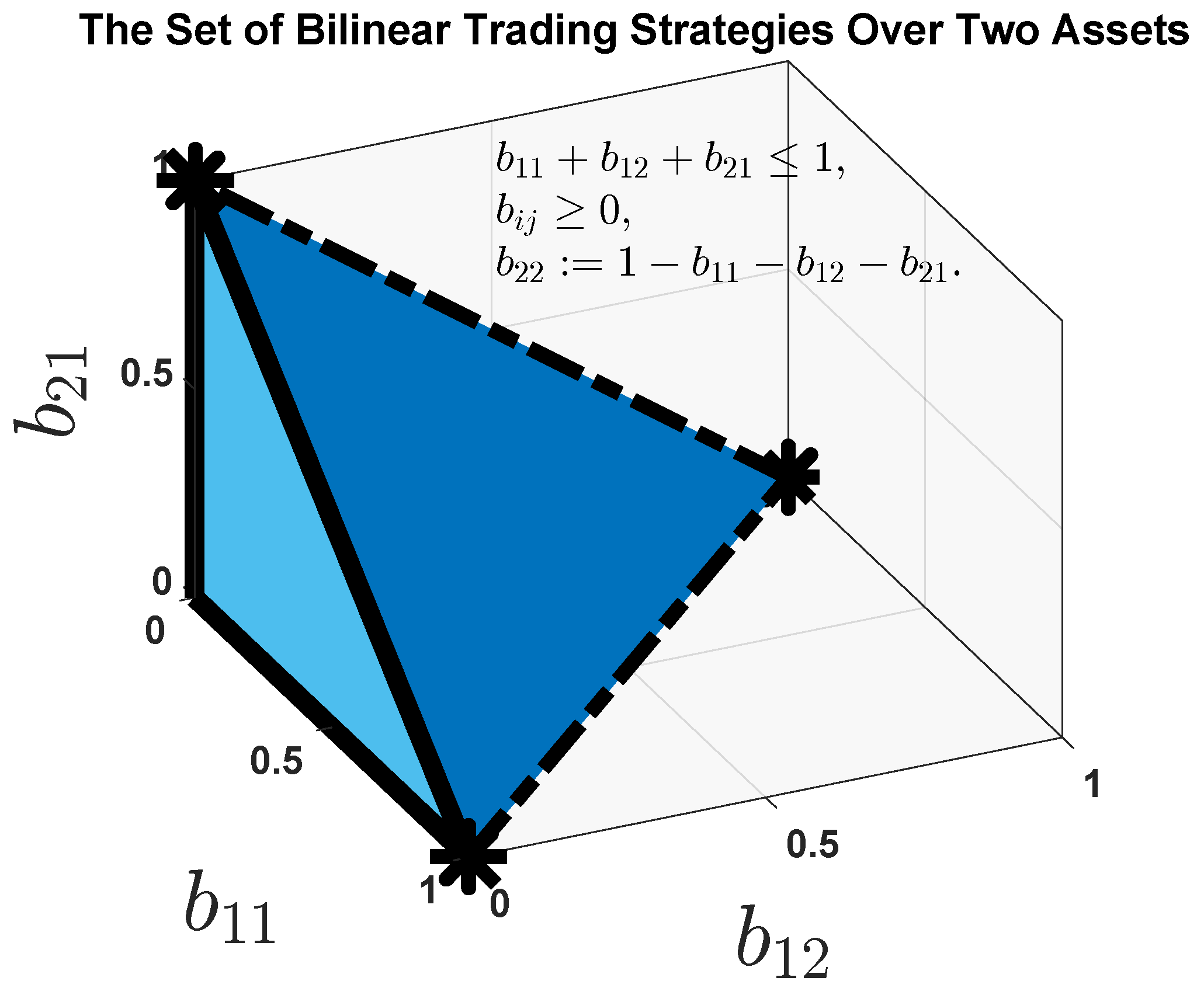
To close out the paper, this subsection provides exact formulas for the behavior of the universal bilinear portfolio in the context of our original motivating example (as discussed in the introduction) for the case of $m:=2$ assets. Accordingly, we will assume that asset 2 is cash (which pays no interest) and that asset 1 is a “hot stock” that always doubles in the first half of each investment period and then loses $50\%$ of its value in the latter half of each investment period. Thus, we have the individual return sequence defined by $x_t:\equiv {(2,1)}^{\prime }$ and $y_t:\equiv {(1/2,1)}^{\prime }$. The set of all bilinear trading strategies is now a family of $2\times 2$ matrices

$$\mathcal{B}:=\left\{(b_{11},b_{12},b_{21},b_{22})\in {\mathbb{R}}_{+}^4:b_{11}+b_{12}+b_{21}\le 1,b_{22}=1-b_{11}-b_{12}-b_{21}\right\},$$

(45)

where the variable $b_{22}$ is bound by the relation $b_{22}:=1-b_{11}-b_{12}-b_{21}$. As depicted in Figure 1, this set of matrices amounts to a tetrahedron in ${\mathbb{R}}_{+}^3$.

Analogous to Thomas Cover (1991), we will use the uniform prior density $f(b_{11},b_{12},b_{21})\equiv 6$, e.g., the volume of the tetrahedron $\mathcal{B}$ is given by

$$\mathrm{Volume}\left(\mathcal{B}\right)={\displaystyle \underset{b_{11}=0}{\overset{1}{\int }}} {\displaystyle \underset{b_{12}=0}{\overset{1-b_{11}}{\int }}}{\displaystyle \underset{b_{21}=0}{\overset{1-b_{11}-b_{12}}{\int }}}d{b}_{21}d{b}_{12}d{b}_{11}=\frac{1}{6}.$$

(46)

During each (complete) investment period, the (intra-period) capital growth factor achieved by the bilinear trading strategy B amounts to

$$x_t^{\prime }B{y}_t=\left[\begin{array}{cc}2& 1\end{array}\right]\left[\begin{array}{cc}{b}_{11}& b_{12}\\ b_{21}& 1-b_{11}-b_{12}-b_{21}\end{array}\right]\left[\begin{array}{c}1/2\\ 1\end{array}\right]=1+b_{12}-\frac{b_{21}}{2},$$

(47)

so that $W_B(x^t,y^t)={\left(1+b_{12}-b_{21}/2\right)}^t$. Thus, the universal wealth $\widehat{W}(x^t,y^t)$ that obtains after the elapse of t complete investment periods is found by evaluating the triple integral

$$\begin{array}{c}6{\displaystyle \underset{b_{11}=0}{\overset{1}{\int }}} {\displaystyle \underset{b_{12}=0}{\overset{1-b_{11}}{\int }}}{\displaystyle \underset{b_{21}=0}{\overset{1-b_{11}-b_{12}}{\int }}}{\left(1+b_{12}-\frac{b_{21}}{2}\right)}^{t}d{b}_{21}d{b}_{12}d{b}_{11}\hfill \\ \hfill =\frac{2^{t+5}-12(t+2)-2^{1-t}}{(t+1)(t+2)(t+3)}\sim \frac{32}{t^3}·2^t.\end{array}$$

(48)

The best bilinear trading strategy in hindsight is obviously

$$B^{*}(x^t,y^t)\equiv \left[\begin{array}{cc}0& 1\\ 0& 0\end{array}\right],$$

(49)

e.g., the extremal strategy that bets the ranch on the stock in the first half of each investment period, and then cashes out completely in the latter half of each investment period. This (perfect trading) yields the hindsight-optimized wealth $D(x^t,y^t)=D(x^t,y^{t-1})=2^t$, which corresponds to the asymptotic growth rate $\underset{t\to \infty }{\lim }(1/t)\log D(x^t,y^t)=\log 2=69.3\%$ per complete investment period, compounded continuously. The competitive ratio after t full periods is equal to

$$R(x^t,y^t)=\frac{32-12(t+2)2^{-t}-2^{1-2t}}{(t+1)(t+2)(t+3)}\sim \frac{32}{t^3}.$$

(50)

Note well that Corollary 1 promised us the minorant

$$R(x^t,y^t)\ge \frac{6}{(t+1)(t+2)(t+3)},$$

(51)

which is indeed correct; we of course have $\underset{t\to \infty }{\lim }(1/t)\log R(x^t,y^t)=0$, so that the universal bilinear portfolio compounds its money at the same asymptotic rate as the best bilinear trading strategy in hindsight.

Against this individual return sequence, the universal bilinear portfolio finds its expression in the triple integral

$$\frac{6}{\widehat{W}(x^t,y^t)}{\displaystyle \underset{b_{11}=0}{\overset{1}{\int }}} {\displaystyle \underset{b_{12}=0}{\overset{1-b_{11}}{\int }}}{\displaystyle \underset{b_{21}=0}{\overset{1-b_{11}-b_{12}}{\int }}}{\left(1+b_{12}-\frac{b_{21}}{2}\right)}^t\left[\begin{array}{cc}{b}_{11}& b_{12}\\ b_{21}& 1-b_{11}-b_{12}-b_{21}\end{array}\right]d{b}_{21}d{b}_{12}d{b}_{11}.$$

(52)

With some effort, one can explicitly evaluate the on-line bilinear weights, as follows:

$${\widehat{b}}_{11}(x^t,y^t)=\frac{2·4^{t+2}-3·2^t(t^2+5t+10)+1}{(t+4)[4^{t+2}-3·2^{t+1}(t+2)-1]}\sim \frac{2}{t}\to 0,$$

(53)

$${\widehat{b}}_{12}(x^t,y^t)=\frac{2^{t+4}(3t-4)+18(t+4)+2^{-t}}{3(t+4)[2^{t+4}-6(t+2)-2^{-t}]}\to 1,$$

(54)

$${\widehat{b}}_{21}(x^t,y^t)=\frac{2^{t+6}-36(t+1)-2^{-t}(3t+19)}{3(t+4)[2^{t+4}-6(t+2)-2^{-t}]}\sim \frac{4}{3t}\to 0,$$

(55)

$${\widehat{b}}_{22}(x^t,y^t)={\widehat{b}}_{11}(x^t,y^t)\sim \frac{2}{t}\to 0.$$

(56)

Notice that the $(1,1)$ and $(2,2)$ extremal strategies (which both amount to buy-and-hold strategies) are assigned equal weights by the universal bilinear portfolio (in the sense that ${\widehat{b}}_{22}={\widehat{b}}_{11}$); this happens on account of the fact that both assets produce identical results for a buy-and-hold investor over any complete investment period.

Thus, the universal bilinear portfolio learns to trade perfectly in as much as

$$\underset{t\to \infty }{\lim }\widehat{B}(x^t,y^t)=\left[\begin{array}{cc}0& 1\\ 0& 0\end{array}\right].$$

(57)

The same cannot be said for the universal 1-linear portfolio, which achieves the capital growth factor12

$$\begin{array}{cc}\widehat{S}(x^t,y^t)\hfill & ={\displaystyle \underset{c=0}{\overset{1}{\int }}}{(1+c)}^t{(1-c/2)}^{t}dc\hfill \\ \hfill & ={\displaystyle \sum _{k_1=0}^t}{\displaystyle \sum _{k_2=0}^{t-k_1}}\left(\genfrac{}{}{0pt}{}{t}{k_1,k_2,t-k_1-k_2}\right)\frac{{(-1)}^{k_2}}{2^{k_1+k_2}(k_1+2k_2+1)}.\hfill \end{array}$$

(58)

After t complete investment periods, the best constant-rebalanced portfolio in hindsight is equal to ${(1/2,1/2)}^{\prime }$, which corresponds to the (sub-optimal) bilinear trading strategy $B=\left[\begin{array}{cc}1/4& 1/4\\ 1/4& 1/4\end{array}\right].$ The final wealth of the best constant-rebalanced portfolio in hindsight is thereby $S^{*}(x^t,y^t)={(9/8)}^t$. Thus, the excess asymptotic growth rate of the universal bilinear portfolio (over and above that of the universal 1-linear portfolio) is $\log 2-\log (9/8)=57.5\%$ per (complete) investment period, compounded continuously.

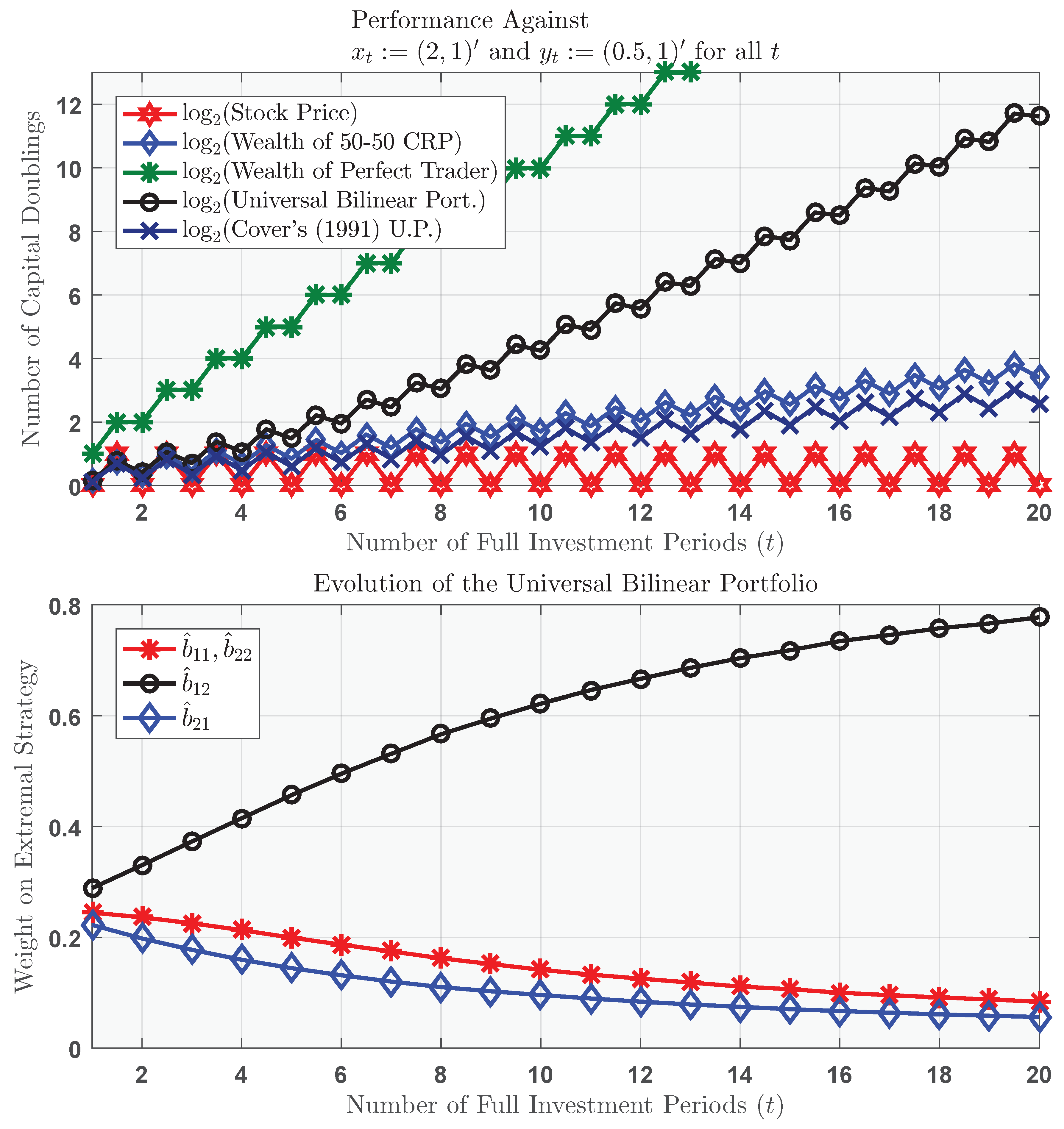
For the sake of visualization, Figure 2 plots the bankroll of the universal bilinear portfolio in comparison to that of the universal 1-linear portfolio and the wealth achieved by a perfect trader. The lower panel illustrates the parameter learning that obtains from the performance-weighted average of all bilinear trading strategies.

4. Summary and Conclusions

In this note, we constructed a neat application and extension of the brilliantly lucid Ordentlich-Cover theory of “universal portfolios”. The original (1-linear) universal portfolios guarantee to achieve a high percentage of the final wealth that would have accrued to the best constant-rebalanced portfolio in hindsight for the actual (realized) sequence of asset prices.

The constant-rebalanced portfolios constitute a very simple parametric family of active trading strategies, where the “activity” amounts to continuously executing rebalancing trades so as to restore the portfolio to a given target allocation. Inspired by the fact that a constant-rebalanced portfolio is a (horizon-1) trading strategy whose capital growth factor in any given period is a linear function of the market’s gross return vector, we decided to consider the wider class of bilinear trading strategies (or bilinear portfolios), which are mini 2-period active strategies whose capital growth factors are linear separately in the two gross return vectors.

Accordingly, we hit upon the more powerful benchmark of the best bilinear trading strategy in hindsight for the actual sequence of asset prices. This led us to apply Cover’s ingenious (Cover 1991) performance-weighted averaging technique to this new situation, e.g., the universal bilinear portfolio is a performance-weighted average of all possible bilinear trading strategies.

Applying Cover and Ordentlich’s elegant (Cover and Ordentlich 1996) methodology, we showed that for any financial market with m assets13, at worst, the percentage of hindsight-optimized wealth achieved by the universal bilinear portfolio will tend to zero like the quantity $T^{-(m^2-1)}$ as $T\to \infty$, where T denotes the number of complete (bipartite) investment periods. Consequently, the universal bilinear portfolio succeeds in matching the performance of the best bilinear trading strategy in hindsight to “first order in the exponent,” e.g., the excess continuously-compounded per-period capital growth rate of the best bilinear trading strategy in hindsight converges (uniformly) to zero, regardless of the individual sequence of asset prices.

Thus, we showed that the universal bilinear portfolio asymptotically dominates the universal 1-linear portfolio in the same technical sense that the universal 1-linear portfolio asymptotically dominates all constant-rebalanced portfolios and all buy-and-hold strategies. The universal bilinear portfolio will beat the universal 1-linear portfolio by an exponential factor, provided that the individual sequence of asset prices enjoys the property that the best bilinear trading strategy in hindsight achieves an asymptotic growth rate that is strictly greater than that of the best constant-rebalanced portfolio in hindsight.

Analogously, we can get carried away and define the concept of a trilinear trading strategy $B:={\left(b_{ijk}\right)}_{i,j,k=1}^m$, whose (horizon-3) capital growth factor in any (tripartite) period t is equal to the trilinear form

$${\langle x_t,y_t,z_t\rangle }_B:={\displaystyle \sum _{i=1}^m}{\displaystyle \sum _{j=1}^m}{\displaystyle \sum _{k=1}^m}{b}_{ijk}{x}_{ti}{y}_{tj}{z}_{tk},$$

(59)

where $b_{ijk}\ge 0$ and ${\displaystyle \sum _{i=1}^m}{\displaystyle \sum _{j=1}^m}{\displaystyle \sum _{k=1}^m}{b}_{ijk}=1$. This leads to a universal trilinear portfolio whose worst-case competitive ratio behaves like $T^{-(m^3-1)}$ as $T\to \infty$. In general, an H-linear trading strategy (cf. with Garivaltis (2018b)) divides each period t into H sub-periods, wherein the gross return vectors are denoted $(x_t^1,x_t^2,...,x_t^h,...,x_t^H)={\left(x_t^h\right)}_{h=1}^H$. Intra-period capital growth is now generated by the H-linear form (cf. with Serge Lang (1987))

$${\langle x_t^1,...,x_t^H\rangle }_B:=\sum _{(i_1,...,i_H)\in {\{1,...,m\}}^H}\left\{B(i_1,...,i_H){\displaystyle \prod _{h=1}^H}{x}_{t{i}_h}^h\right\},$$

(60)

where $B(i_1,...,i_H)\ge 0$ and ${\displaystyle \sum _{(i_1,...,i_H)\in {\{1,...,m\}}^H}}B(i_1,...,i_H)=1$; the attendant universal H-linear portfolio asymptotically achieves, at worst, the fraction $T^{-(m^H-1)}$ of the final wealth of the best H-linear trading strategy in hindsight.

Hence, one can use this method to construct an endless hierarchy of ever more dominant universal portfolios. If the horizon $H_2$ is an integer multiple of the horizon $H_1$, say $H_2:=q·H_1$, then the act of repeating a given $H_1$-linear portfolio B for q times in succession constitutes a special type of $H_2$-linear portfolio; the universal $H_2$-linear portfolio thereby asymptotically outperforms the universal $H_1$-linear portfolio “to first order in the exponent,” á la Cover.

Disclosures

This paper is solely the work of the author, who declares that he has no conflicts of interest; the work was funded entirely through his regular academic appointment at Northern Illinois University.

References

- Bell, R. M., and T. M. Cover. 1980. Competitive Optimality of Logarithmic Investment. Mathematics of Operations Research 5: 161–66. [Google Scholar] [CrossRef]
- Bell, R. M., and T. M. Cover. 1988. Game-Theoretic Optimal Portfolios. Management Science 34: 724–33. [Google Scholar] [CrossRef] [Green Version]
- Black, Fischer, and Myron Scholes. 1973. The pricing of options and corporate liabilities. Journal of Political Economy 81: 637–54. [Google Scholar] [CrossRef] [Green Version]
- Breiman, Leo. 1961. Optimal Gambling Systems for Favorable Games. Paper presented at the Fourth Berkeley Symposium on Mathematical Statistics and Probability, Berkeley, CA, USA, June 20–July 30; vol. 1, pp. 63–68. [Google Scholar]
- Cover, Thomas M. 1991. Universal Portfolios. Mathematical Finance 1: 1–29. [Google Scholar] [CrossRef]
- Cover, Thomas M., and David H. Gluss. 1986. Empirical Bayes Stock Market Portfolios. Advances in Applied Mathematics 7: 170–81. [Google Scholar] [CrossRef] [Green Version]
- Cover, Thomas M., and Erik Ordentlich. 1996. Universal Portfolios With Side Information. IEEE Transactions on Information Theory 42: 348–63. [Google Scholar] [CrossRef] [Green Version]
- Cover, Thomas M., and Joy A. Thomas. 2006. Elements of Information Theory. Hoboken: John Wiley & Sons. [Google Scholar]
- Curatola, Giuliano. 2019. Portfolio Choice of Large Investors Who Interact Strategically. Working Paper. Siena: University of Siena. [Google Scholar]
- Garivaltis, Alex. 2018a. Game-Theoretic Optimal Portfolios in Continuous Time. Economic Theory Bulletin 7: 235–43. [Google Scholar] [CrossRef] [Green Version]
- Garivaltis, Alex. 2018b. Multilinear Superhedging of Lookback Options. Working Paper. DeKalb: Northern Illinois University. [Google Scholar]
- Garivaltis, Alex. 2019a. Game-Theoretic Optimal Portfolios for Jump Diffusions. Games 10: 8. [Google Scholar] [CrossRef] [Green Version]
- Garivaltis, Alex. 2019b. Exact Replication of the Best Rebalancing Rule in Hindsight. The Journal of Derivatives 26: 35–53. [Google Scholar] [CrossRef]
- Kelly, John L. 1956. A New Interpretation of Information Rate. The Bell System Technical Journal 35: 917–26. [Google Scholar] [CrossRef]
- Lang, Serge. 1987. Linear Algebra. New York: Springer. [Google Scholar]
- Latané, Henry Allen. 1959. Criteria for Choice Among Risky Ventures. Journal of Political Economy 67: 144–55. [Google Scholar] [CrossRef]
- MacLean, Leonard C., Edward O. Thorp, and William T. Ziemba. 2011. The Kelly Capital Growth Investment Criterion: Theory and Practice. Hackensack: World Scientific Publishing Company. [Google Scholar]
- Ordentlich, Erik, and Thomas M. Cover. 1998. The Cost of Achieving the Best Portfolio in Hindsight. Mathematics of Operations Research 23: 960–82. [Google Scholar] [CrossRef] [Green Version]
- Samuelson, Paul A. 1963. Risk and Uncertainty: A Fallacy of Large Numbers. Scientia 6: 153–58. [Google Scholar]
- Samuelson, Paul A. 1969. Lifetime Portfolio Selection by Dynamic Stochastic Programming. Review of Economics and Statistics 51: 239–46. [Google Scholar] [CrossRef]
- Samuelson, Paul A. 1979. Why We Should not Make Mean Log of Wealth Big Though Years to Act are Long. Journal of Banking and Finance 2: 305–7. [Google Scholar] [CrossRef]
- Tal, O., and T. D. Tran. 2020. Adaptive Bet-Hedging Revisited: Considerations of Risk and Time Horizon. Bulletin of Mathematical Biology 82: 1–32. [Google Scholar] [CrossRef] [PubMed] [Green Version]
- Thorp, Edward O. 1969. Optimal Gambling Systems for Favorable Games. Revue de l’Institut International de Statistique 37: 273–93. [Google Scholar] [CrossRef]
- Widder, David Vernon. 1989. Advanced Calculus. New York: Dover Publications. [Google Scholar]