
Nonprofits and Pass-Throughs: Performance Comparison


School of Business, Washburn University, 1700 SW College Ave, Topeka, KS 66621-1117, USA
*
Author to whom correspondence should be addressed.
Int. J. Financial Stud. 2021, 9(1), 13; https://0-doi-org.brum.beds.ac.uk/10.3390/ijfs9010013
Submission received: 15 November 2020
/
Revised: 9 February 2021
/
Accepted: 22 February 2021
/
Published: 27 February 2021
(This article belongs to the Special Issue Practical Applications of Capital Structure Models)
Abstract
:This paper’s purpose is to compare nonprofits with pass-throughs in terms of valuation, leverage, and growth. To achieve this purpose, we use the Capital Structure Model. This model determines maximum firm valuation through incorporating real data (tax rates, credit spreads, and historical growth rates). Since this is the first study to offer our particular set results on valuation, leverage and growth, our findings are value-additive in terms of the comparative research on nonprofits and pass-throughs. The new and scientific value of our findings are further established by robust tests that modify values for key variables. Major findings include the following. Nonprofits have over a fifty percent valuation advantage over pass-throughs and achieve a four times greater increase in dollar value when going from nongrowth to growth. The latter accomplishments are attained with a smaller before-tax plowback ratio and less retained earnings. Such achievements occur because nonprofits are not taxed on earnings retained for growth. While nonprofits have somewhat greater optimal leverage ratios than pass-throughs, they gain a bit less in dollars added from debt unless growth rates increase as projected when tax rates are lowered. Nonprofits gain less percentage-wise from debt because their unlevered firm value is greater than pass-throughs.
JEL Classification:
G32; G35; L31; L3331. Introduction
Prior Capital Structure Model (CSM) research examines C corp (CC) and pass-through (PT) ownership forms (Hull and Price 2015; Hull 2020b; Hull and Hull 2020). This paper extends this research by being the first CSM study to investigate nonprofits (NPs). While NPs are not profit-driven, they share characteristics similar to the for-profit (FP) ownership forms of PT and CC. For example, both NPs and FPs are primarily composed of small-sized entities. In addition, since NPs depend on FPs for funding, one can argue that both NPs and FPs have their welfare influenced by the same market forces. Furthermore, NPs and FPs can be competitors within the same industry. A case in point in the healthcare industry where NPs and FPs supply the same services and compete for the same customers. Both NPs and FPs are alike in producing financial statements that report assets, liabilities, revenues, and expenses. For NPs, revenues come mainly from services, contributions, grants, and investments in riskless and risky assets. According to the comparative evidence given by Anheier (2014), services (through the fees collected) is the largest component of NP revenue. For PTs, revenues come from services, sales, and investments in riskless and risky assets. Finally, both NPs and FPs have payroll taxes but only PTs pay business income tax with an exception being that some NPs pay business income tax on small commercial endeavors such as gift shops.
This study’s major purpose is to compare NPs with PTs where the latter is the dominant FP ownership form in terms of the quantity of outstanding companies, number of employees, and amount of revenue produced. According to Hull and Hull (2020), PTs pay about 2.3 more in federal taxes than CCs. Our research goal aims at determining how differences in the taxing of NPs and PTs, when all else is equal, affect their performance as measured by debt choice, valuation, leverage gain, and growth-related outcomes. The differences in the taxation policies governing NPs and PTs can be described as nearly polar opposites in that NPs receive three major tax benefits unavailable to PTs. First, NPs are tax-exempt, which means they can avoid the PT forms of taxes such as federal, state, county, municipal, property, and sales. For this study, we focus on differences in federal taxes between NPs and PTs. Second, unlike PTs, NPs do not have monetary payouts to equity owners in the form of cash distributions and taxable capital gains. Third, since NPs issue tax-exempt debt, its debtholders can circumvent the taxes paid on interest income by PT debt owners. To illustrate the nature of tax-exempt debt ownership, NPs seek financing through municipal bonds that are issued by states and municipalities. These bonds are tax-exempt for the bondholders unless more than 5% of proceeds are used for profitable activities, which is highly unlikely. In conclusion, NPs are in a position to avoid all forms of taxes paid by PTs except payroll taxes.
To achieve our research goal, we use the CSM (Hull 2018; Hull 2019) as our method to determine optimal outcomes for NPs and PTs. The CSM allows us to compute firm value for increasing debt-for-equity choices tied to credit ratings of decreasing quality. From these computations, we can determine the maximum firm value (max VL) and thus identify the optimal debt-to-firm value ratio (ODV) that, in turn, is aligned with an optimal credit rating (OCR). The key to these computations is the assumption of analogous risk classes. As NPs are subsidized by PTs, their revenue streams are influenced by the same economic factors and thus capable of having similar risk classes. The assumption of parallel risk classes for NPs and PTs implies the same costs of borrowing. For our tests, costs of borrowing are based on credit spreads matched to bond ratings and interest coverage ratios (ICRs). The same borrowing costs for NPs and PTs enable the CSM to compute outcomes so that comparisons can be made and conclusions can be drawn that are based on different tax rates.
Four arguments support the notion that the outcomes for NPs and PTs can be based on analogous risk classes. First, as illustrated previously with the healthcare industry, there exists businesses that can choose between being a NP or PT and for which they compete for producing the same goods and services. Second, NPs and PTs are of similar sizes as both consist largely of small organizations while having large entities that dominate in terms of revenue and expenses. Third, NPs and PTs are both affected by market conditions as NPs are dependent on funding that is provided by FP businesses and their employees. Even government funding for NPs is dependent on FPs paying taxes. Fourth, like revenues for PTs, charitable contributions received by NPs also decline during an economic recession such as is triggered by a financial crisis.
For our growth tests that use the historical growth rate of 3.12% and Tax Cuts and Jobs Act (TCJA) tax rates for both NPs and PTs, we offer the below findings that are the composites of tests using data for the two most recent years available at the time of this study, namely, 2018 and 2019. To our knowledge, our findings are new as the comparative research on NPs versus PTs is virtually nonexistent in terms of the outcomes we examine. These findings, that are supported by robust tests (so as to further establish their scientific value), are as follows.
First, we document that ODV is 12.27% higher for NPs compared to PTs indicating that NPs need to use more debt to reach maximum firm value (max VL). Second, while we know that NPs have a significant valuation advantage by not paying taxes, we reveal the extent of this advantage by showing that max VL for NPs is 51.63% higher than PTs. Third, we show that growth helps nongrowth NPs more than nongrowth PTs in increasing max VL. To illustrate, NPs achieve a 13.83% increase when going from their nongrowth max VL to their growth max VL while PTs only attain a 3.42% rise.
Fourth, NPs achieve their increase in value from growth with a before-tax plowback ratio (PBRBT) that is 26.63% smaller than PTs and an unlevered growth rate (gU) that is 7.97% lower than PTs. The latter two results occur because PBRBT and gU are positively related to retained earnings (RE) and PTs can only use RE after business taxes are paid on it while NPs avoid business taxes. Fifth, while NPs increase their value more than PTs when going from their nongrowth max VL to their growth max VL, a different picture emerges when going from their unlevered firm value (EU) with growth to their max VL with growth. For example, in terms of the maximum gain to leverage (max GL), NPs gain 2.25% less in absolute dollars by issuing debt compared to PTs. This can be explained by not having an interest tax shield, which is a key valuation component of mainline capital structure theory. While this finding is supported, on average, by robust tests, these tests indicate a great variability in outcomes. In particular, greater growth rates cause NPs to gain more and not less.
Sixth, in terms of the maximum percent change in unlevered equity value (max %∆EU) from a debt-for-equity transaction, we find that NPs increase 4.57% from their unlevered equity value with growth while PTs increase 7.29% from their unlevered equity value with growth. This finding is supported by robust tests including those with greater growth. Seventh, with regard to the net benefit from leverage (NB), we find that EU for NPs rises 15.93% for every dollar of debt while EU for PTs increases 27.96%. Thus, while this indicates that NPs are less efficient in their use of each dollar of debt, it also reflects the fact that NPs not only have greater ODVs but also have higher firm valuations and so must issue more debt to attain the same optimal credit rating (OCR). For both NPs and PTs, OCR is Moody’s rating of A3.
The remainder of this paper is as follows: In Section 2, we discuss the two ownership categories of NP and PT; examine the nature of equity and debt for NPs and PTs; assign tax rates for NPs and PTs tests; and discuss capital structure models. Section 3 presents our methodology, explains how we identify the optimal debt-for-equity choice, reviews the CSM approach to growth, and provides the procedure to get leverage choices and the costs of borrowing based on credit spreads assigned to credit ratings. Section 4 introduces variables and computations and offers illustrations of NP and PT outcomes using our low (L) tax rates under TCJA with a historical growth rate of 3.12%. From these tests, we present figures that graphically display results. Section 5 provides robust results that incorporate high (H) tax rates, pre-TCJA tax rates, and increased growth under TCJA. These results include comparing outcomes for NPs and PTs for different credit spreads that can be found from 2014‒2019 with our focus on the two most recent years of 2018 and 2019. Section 6 summarizes our main findings. Due to the large number of abbreviations, Appendix A provides information on the acronyms used in the paper.
2. Background and Literature Review
This section begins by providing background information on the following: ownership categories of nonprofits (NPs) and pass-throughs (PTs); sources of equity and debt financing for NPs and PTs; tax rates applicable to NPs and PTs. We then provide a literature review of capital structure models.
2.1. Key Features of Nonprofits (NPs) and Pass-Throughs (PTs)
Exhibit 1 summarizes key features for the ownership categories of NPs and PTs. The Major Goal row of the Nonprofit column states that NPs have a major goal of maximizing service distributions. In contrast, the Pass-Through column for this row says that PTs seek to maximize monetary distributions. While these goals appear to be different, they have a common interwoven theme of value in the sense that services have a monetary value. The Equity Distributions row captures the same theme. NP equity distributions refer to services rendered, while PT equity distributions refer to cash payouts and capital gains.
Of importance to this paper is the role of taxes as represented in the last five rows of Exhibit 1. The two rows on personal taxes provide an indicator of the after-tax valuation advantage of NPs over PTs. As seen in the last row, only PTs provide a substantial interest tax shield (ITS). However, NPs offset this ITS disadvantage (as seen in the Sources of Debt Financing row) by being able to issue personal tax-exempt debt (such as local and state government bonds). Thus, NPs will avoid taxable debt (such as bank debt) because it is more expensive. While C corps (CCs) pay both corporate taxes on earnings and personal taxes on distributions and capital gains, a PT only pays personal taxes on earnings albeit their personal tax rate is noticeably higher with a maximum statutory tax rate of 0.37 compared to the maximum personal tax rate of 0.20 paid by most CC owners on qualified dividends and capital gains. With the passage in December 2017 of the Tax Cuts and Jobs Act (TCJA), the maximum CC tax rate of 0.35 fell to a flat rate of 0.21, which is a large decline of 0.14. In contrast, the maximum for PTs only fell from 0.396 to 0.37, which is drop of just 0.026. TCJA caused other changes that affect PTs (and other individual personal income tax filers) in positive and negative ways with these changes often serving to offset one another.
Despite their tax differences, NPs and PTs can be similar in important characteristics. First, some enterprises can choose to be either an NP or a PT implying they can be substitute ownership types. DeSimone (2019) writes that LLCs can be NPs albeit the process is complex. Keatinge (2009) adds that LLCs have statutes that allow them to become NPs. In addition, within industries like the health care industry, NPs coexist with all types of PTs (sole proprietorships, partnerships, S corps, LLCs, and LLPs) with NPs and PTs supplying the same goods and services.
Second, like most PTs (exceptions are large publicly traded PTs), NPs are not publicly traded and so market risk, as represented by the CAPM beta, cannot be directly computed from empirical data. Regardless, NPs and PTs are affected by market conditions as their well-beings are altered when factors affecting market conditions change. For example, large NP donors give through incomes tied to their for-profit businesses and market investments. Furthermore, another major source of income for NPs is their investment portfolios that can be significantly invested in the stock market and so involve assets subject to market risk.
Third, since market risk affects NPs and PTs, they are both susceptible to other risks involving interest rate, exchange rate, geopolitical events, and recessions. In regard to recessionary risk, charitable contributions received by NPs decline when businesses falter during an economic recession such as is caused by a financial crisis (banking panics, stock market crash, currency crises, sovereign defaults), an external trade shock, an adverse supply shock, the bursting of an economic bubble, or a large-scale natural or anthropogenic disaster. Thus, NPs and PTs share in classifications of risks that all enterprises face be they operational and financial risk or other lesser mentioned risk types such as competitive, compliance, legal, reputational, quality, credit, resource, and seasonal. Given the similar exposure of NPs and PTs to all forms of risk, our tests assume that NPs and PTs can inhabit similar risk classes and thus can share in the same costs of borrowing.
Fourth, while both NPs and PTs can be quite large, both also consist primarily of smaller enterprises. In fact, the vast majority of for-profits (FPs) are small businesses, whether they are PTs or CCs (although the latter have many larger firms). Brookings (2017) reports that 99% of FPs have less than USD 10 million in revenues with most of these FPs consisting of sole proprietorships that are PT businesses owned by one person. Other types of PTs (partnerships, LLCs, and S corps) can be extremely large. The Tax Policy Center (2018) notes that the 33.7 million PTs in 2016 have USD 957 billion in net income (average of USD 28,398). This is broken down as follows. First, the 25 million sole proprietors (nonfarm) report net income of USD 328 billion (average of USD 13,120). Second, the 8.7 million partnerships and S corporations report USD 629 billion in net income (average of USD 72,299). Like PTs, NPs are predominantly small. According to the National Center for Charitable Statistics, NCCS, (National Center for Charitable Statistics 2018), there are more than 1.5 million NPs registered in the US, including public charities, private foundations, and other organizational classifications. Contributions to different charities reached USD 358.38 billion in 2014 (with an average contribution of USD 238,920). NCCS writes that even after excluding NPs with gross receipts below the USD 50,000 filing threshold, the remaining two-thirds of NPs in 2015 contain 210,670 public charities with less than USD 500,000 in expenses (revenues average about 7.5% greater than expenses). These 210,670 NPs compose less than two percent of total public charity expenses of USD 32.3 billion. NPs with USD 10 million or more in expenses include about 5% of total public charities but account for nearly 88% of public charity expenses of USD 1.6 trillion.
2.2. Equity and Debt Financing for Nonprofits (NPs) and Pass-Throughs (PTs)
NP researchers (Bowman 2002; Miller 2003; Jegers and Verschueren 2006; Calabrese 2011) speak of NP borrowings in the same terms as the two general FP types of financing: equity and debt. Below we discuss these types.
Under the Sources of Equity Financing heading in Exhibit 1, we find that internal equity and external equity are given as the two major sources of equity financing for both NPs and PTs. For our purposes, internal equity refers to cash flows generated by an enterprise and set aside for growth before any applicable taxes are supplied. For NPs, internal equity includes unrestricted cash flows or cash flows earmarked for growth in the form of eligible revenues and investment/endowment income while external equity include cash inflows for growth from contributions, grants, and government sources. The equity financing sources for NPs are subject to debate by researchers as to whether they are internal or external or even if they are equity financing. For example, the external equity financing source of contributions (e.g., donations/gifts) might better be classified as eligible revenues. Bowman (2002) is among those who discuss the nature of contributions. For PTs, internal equity includes retained earnings while external equity consists of new partnerships, new issuances (by large PTs), and venture capital.
Under the Sources of Debt Financing heading for NPs, Exhibit 1 reports that debt can be classified as (i) tax-exempt for which no personal taxes exist, (ii) nonfinancial debt (consisting of mortgages that serves the same purpose as long-term financial debt,) and (iii) short-term debt (mostly trade credit as bank borrowings are avoided). Bowman (2015) cites 2012 data from the NCCS that report that tax-exempt debt composes nearly two-thirds of the long-term debt for NPs. Calabrese and Ely (2016) point out that there has been a twenty-year trend during which NPs have taken on more tax-exempt debt. While NPs can have bank debt, they will go to great lengths to avoid these borrowings since bank debt is not tax-exempt and therefore costlier. Similar to trade credit is a line of credit with a bank that NPs (like PTs) can use to cover the gaps in irregular monthly income. Under the Sources of Debt Financing heading for PTs, Exhibit 1 reports the debt can be classified as bond issues, mezzanine debt, Small Business Administration loans, and short-term debt. These PT debt sources are not tax-exempt.
In terms of comparing financing forms between NPs and FPs, the literature is sparce focusing on the heathcare industry. For this industry, NPs and FPs coexist where FPs can include both PTs and CCs healthcare organizations. For example, Trussell (2012) notes that the NP and FP ownership forms have unique financing mechanisms. However, these differences do not impact the relative amount of debt and equity in their capital structures. The latter is consistent with our findings.
2.3. Assignment of Unlevered and Levered Tax Rates for Nonprofits (NPs) and Pass-Throughs (PTs)
Prior to the lowering of FP tax rates by TCJA, Pomerleau (2015) writes that PTs faced an effective (or average) total tax rate of 0.47 that includes federal taxes and non-federal taxes such as state, county, municipal, property, sales, and payroll. In regard to the latter, NPs disburse payroll taxes like all FPs. Payroll taxes are the largest component of the non-federal taxes paid by PTs. For states without taxes, PTs do not pay state taxes and so resemble NPs in terms of state taxes paid. For our tests, we only consider federal taxes as described in Section 3.1.
When we cover our gain to leverage (GL) equations in our methodology section, we present unlevered and levered federal equity tax rates where the subscript “1” indicated an unlevered tax rate and the subscript “2” indicates a levered tax rate. Thus, for what follows TC1, TE1, and TD1 are unlevered corporate, personal equity, and personal debt tax rates at the federal level, while TC2, TE2, and TD2 are the corresponding levered tax rates that change with leverage as described by Hull (2014). By definition, unlevered refers to no debt. With this in mind, our use of the unlevered debt tax rate of TD1 is only for practically purposes as we need a starting point for the debt tax rate that rises with leverage. For CSM papers, where TD1 is not emphasized as a starting point, TD2 is simply called TD.
Before the reduction by TCJA in the personal levered equity tax rate (TE2), the Tax Policy Center (2016) noted that over two-thirds of PTs are taxed at either the maximum federal tax rate of 0.396 or the 0.28 alternative minimum rate. The average of these two rates generates a TE2 of 0.338. The Small Business Administration (SBA Office of Advocacy 2009), the National Federation of Independent Business (2013), and the Tax Policy Center (2018) indicate that most PTs experience a TE2 below 0.3 indicating a median would fall below 0.3. However, according to the Brookings (2017), almost half of PT income comes from businesses with an TE2 near the TCJA maximum. Considering all sources and the recent fall in TE2 under TCJA an effective TE2 between 0.21 and 0.34 is a reasonable ballpark estimate for TCJA tests. As we begin with an unlevered firm and allow tax rates to change when debt increases as described by Hull (2014), our tests use a personal unlevered equity tax rate (TE1) that is greater than an effective levered TE2 achieved at the optimal debt-to-firm value ratio (ODV).
The key tax rate for this study’s purposes is the business tax rate. For NPs, tax rates are only relevant if an NP happens to have a minor for-profit venture on the side. Under this assumption, the CC business tax rate is used albeit small. If small business ventures are not assumed, we use zero tax rates and so the FP ownership type (CC or PT) is irrelevant. For PT tests, the personal tax rate paid by PT owners is the business tax rate. For our low (L) tax rate tests under TCJA, we use an unlevered TE1 of 0.30 for PTs. This usage enables us to achieve an effective levered TE2 that is near 0.255 at ODV where TE2 changes by 0.03 in its predicted direction for each increasing debt-for-equity choice. As described later, each of our fifteen increasing debt-for-equity choices corresponds to a fall in the quality of one of the fifteen credit ratings given by Damodaran (2020).
Besides an L PT business personal tax rate, our tests include a high (H) PT business personal tax rate. This rate is suggested by Hull (2019) where the unlevered TE1 is 0.36 and the effective levered TE2 is around 0.31 at ODV. An H tax rate gives greater weight to averages whereas an L tax rates provides a greater weight to medians. The above L and H tax rates occur under TCJA tax laws. Thus, tests using these tax rates under TCJA can be referred to simply as TCJA tests. When testing pre-TCJA tax rates, we increase our TCJA unlevered and effective levered TE2 values by 0.02 for both the L and H tax rate tests given that TCJA drops rates for its tax brackets by about 0.02 on average. Tax rates for our L tax rate tests under TCJA are used in the first five tables and first five figures, while tax rates for our robust tests (that include L tax rate tests for a pre-TCJA tax environment and H tax rate tests for both pre-TCJA and TCJA tax environments) are used in the last three tables and the last five figures. In addition, these last tables and figures incorporate a greater growth rate (as discussed later).
Interest distributions for a PT debt owner are taxed at the levered personal debt tax rate (TD2). If debt is held longer than three years, any capital gains are taxed at the lower capital gains rate with a typical maximum rate of 0.20 for which we expect a TD2 around 0.16. A marginal TD2 based on the imputed rate from the highest rated municipal and corporate bond yields varies over times and can be near the maximum statutory rate. However, this imputed tax rate is more of a marginal tax rate than an effective tax rate. Considering all factors, a range from 0.16 to 0.26 is feasible for an average TD2. For our TCJA tests where TD2 increases with leverage, we set the unlevered TD1 at 0.18 to get a levered TD2 around 0.21 at ODV. For our pre-TCJA tests, we increase TD1 by 0.01 due to expectations of slightly greater rates on debt income. We use the same TCJA and pre-TCJA values for TD1 and TD2 for both our L and H tax rate tests as the focus is on the business tax rate that directly impacts (i) internal growth that stems from the use of retained earnings (RE) and (ii) the ITS that results in tax savings at the business tax rate level.
Except for occasional ventures that produce negligible taxable income, we view NPs as having zero tax rates at the corporate and/or personal levels. Since NPs can issue debt that is exempt from personal taxes, it is possible for debtholders to achieve a TD2 of zero. Bowman (2015) writes that most NP debt is tax-exempt. He also notes that the trend has been to issue even more tax-exempt debt. Given the possibility of zero tax rates, our L tax rate tests for NP use zero values for the unlevered corporate tax rate (TC1), TE1, and TD1. Since zero tax rates cannot change with leverage, the levered tax rates of TC2, TE2, and TD2 are also zero. For our H tax rate tests for NPs, we assume tax rates are not zero but small. For these tests, we set both TC1 and TE1 at 0.02 where we assume the existence of minor for-profit ventures (such as gift shops). We set TD1 at 0.04 where we assume some debt is issued that is not tax-exempt. Given that TC1 and TE1 are small, they cannot change much and so achieve similar effective levered tax rates for TC2 and TE2. TD1 is slightly larger and so TD2 is slightly higher at 0.045 since TD2 increases with leverage. For pre-TCJA tests, we increase these unlevered tax rates by 0.01 and achieve effective levered tax rates that have a similar increase. In addition, we set both TC1 and TE1 at 0.03 for pre-TCJA tests and so they both fall so that TC2 and TE2 are both about 0.025. Finally, we set TD1 at 0.05 for pre-TCJA tests and it rises so that TD2 is about 0.06.
Exhibit 2 summarizes the tax rates just discussed. The unlevered tax rates are given first in Nonprofit and Pass-Through columns in each row and are followed by the estimated levered tax rates that occur at ODV. Panel A contains the L tax rates and Panel B provides the H tax rates. The top half of each panel gives the pre-TCJA tax rates and the bottom half reports the TCJA tax rates. While we follow tax laws governing C corps (CCs) for NPs, the results would be similar if we used the tax code governing PTs since all of our NP tests have zero or very small tax rates given their tax-exempt nature. Finally, Exhibit 2 reveals that a main change when going from an L tax rate to an H tax rate is for the business tax rate that affects both growth (through RE) and the ITS where the business tax rate is the personal equity tax rate for PTs and the corporate tax rate for NPs.
2.4. Capital Structure Models
A capital structure model offers an approach to choose among forms of borrowing (and their proportions) that are needed to finance a firm’s operations and growth. The two major forms of borrowing are equity and debt. Trade-off theory (Baxter 1967; DeAngelo and Masulis 1980; Hackbarth et al. 2007; Berk et al. 2010; Hull 2018) posit that there is an optimal amount of equity and debt that maximizes firm value. Key components of trade-off models should capture the positive influence such as exercised by an ITS and the negative influence such as exerted by bankruptcy costs. Trade-off models are consistent with empirical research (Graham 2000; Korteweg 2010; Van Binsbergen et al. 2010) that finds debt increases unlevered firm value.
Agency models provide a trade-off framework where ODV occurs even without an ITS. Jensen and Meckling (1976) demonstrate how maximum valuation occurs at ODV simply from principal-agent valuation effects. As agents of debt owners, equity owners can undertake projects to enhance their residual ownership positions at the expense of debt owners. Besides the negative agency effects on debt owners involving project choice, agency models also detail positive effects when debt enters the capital structure. For example, consider an all-equity firm with a glut of cash flows that leads to managerial squandering. Jensen (1986) contends that such an enterprise can add value by issuing debt because it lessens the cash flows that are being squandered by caretakers.
For large enterprises with many individual owners, there can be almost perfect separation between owners and managers leading to owner-manager conflicts. For PTs that are sole proprietors, these problems do not exist. For PTs that are partnerships, liability is shared among owners ensuring mutual monitoring and less separation of control between owners and managers. For large NPs, the capital is largely supplied by donors who lack the control found in larger for-profits where owners can withdraw assets or sell stocks. However, since NP donors do not have a monetary enrichment motive, agency problems between donors and management can be lessened. Agency costs for NPs can also be lessened in that large donors are often on the board of directors. This helps ensure proper monitoring of the NP management similar to how residual claimants in larger PTs exercise control due to the constant threat that they can sell their ownership claims if managers prove untrustworthy. Despite these arguments that lessen the agency costs for NPs, lack of a clear-cut profit motive that tends to mitigate many agency costs for PTs is not present for NPs. For example, Manne (1999) argues that NPs have greater agency problems because ownership, goals, and performance are less well-defined compared to for-profits like PTs.
In addition to agency models, pecking order models of financing (Donaldson 1961; Myers 1977; Myers and Majluf 1984) do not depend solely on taxes. For PTs, the preference in financing is internal equity (e.g., RE for growth) followed by debt. External equity is the last resort due to expenses especially asymmetric information costs reflected in the negative signaling that accompanies a new issuance. Pecking order models do not address the high after-tax costs experienced by PTs when using internal equity in the form of RE that can only be used after taxes are paid. By paying zero taxes (or negligible amounts of taxes), NPs avoid the taxation on its sources of equity financing. For NPs, as seen earlier in Exhibit 1, internal equity sources earmarked for growth can include eligible revenues and investment/endowment income.
Researchers (Bowman 2002; Calabrese 2011) have applied pecking order theory to NPs. Bowman (2002) suggests that the real cost of NP debt relates to the fear of default because NPs cannot liquidate all of their assets even if on a downward valuation spiral. This means equity forms of financing such as charitable contributions take precedence over debt. Despite the woes associated with debt, Bowman argues that NPs should still prefer debt to asset conversion where asset conversion refers to selling a portion of the endowment. For Bowman, NPs should wait to use endowment funds until they reach their debt restriction as endowment funds used jointly with tax-exempt debt create arbitrage cash flows.
For Calabrese (2011), NPs prefer internal equity in the form of accumulated unrestricted residual revenues over external borrowing. NPs also prefer to maintain some amount of internal pools of capital for future growth. For NPs, internal equity and external funds are not perfect substitutes. The information asymmetries causing the preference for internal equity in the NP sector are different than those found in the FP sector. This is because of less observable benefits to outsiders and variation in donor oversight, willingness, and ability to finance capital.
In this paper, we use the Capital Structure Model (CSM), which is a trade-off model capable of pinpointing a firm’s ODV. The CSM’s focus on internal equity (e.g., RE) is consistent with pecking order models as well as what is observed in the business world where growth is primarily financed by internal equity. For high (H) tests for NPs, that assume a slight amount of taxation beyond zero, we use the CSM equations given by Hull (2018) for CCs. Low (L) tests for NPs offer results that are invariant to the ownership form as all tax rates are zero. For PT tests, we use the CMS equations given by Hull (2019) for both L and H tax rate tests as well as his suggestions concerning values for inputs, especially for H tax rate tests. Values for inputs are also influenced by the recent CSM research (Hull 2020a, 2020b).
3. Methodology
In this section, we present our methodology that consists largely of the Capital Structure Model (CSM). We also include a description of how the CSM is used to identify optimal outcomes. We then present the CSM approach to growth. Finally, we provide the method of obtaining the costs of borrowing using credit spreads that are matched to debt-for-equity choices.
3.1. Capital Structure Model (CSM)
Using the definition that the gain to leverage (GL) = VL − VU where VL is levered firm value consisting of levered equity (EL) and debt (D) and VU is unlevered firm value or, equivalently, unlevered equity value (EU), Hull (2014) extends the CSM research on C corps (CCs) by incorporating changes in tax rates and shows that the nongrowth CC equation is
where
GL = (1 − αIrD/rL)D + (1 − α2rU/rL)EU
αI and α2 capture the effects of effective tax rates with α1 = (1 − TE2)(1 − TC2)/(1 − TD2) and α2 = (1 − TE2)(1 − TC2)/(1 − TE1)(1 − TC1) where TE1 and TE2 are the respective unlevered and levered personal equity tax rates, TC1 and TC2 are the respective unlevered and levered corporate equity tax rates, and TD2 is the debt tax rate, which by definition is a levered tax rate;
rD, rL, and rU, are, respectively, the cost of debt, cost of levered equity, and cost of unlevered equity;
D is the amount of debt issued to retire unlevered equity (EU) with D = (1 − TD2)I/rD where I is the interest payment; and,
EU = (1 − TE1)(1 − TC1)C/rU where C is the before-tax payout with C = (1 − PBRBT)(CFBT) where PBRBT is the before-tax plowback ratio with PBRBT = 0 in (1) due to nongrowth and CFBT is the perpetual before-tax cash flow where equals CFBT = C for nongrowth since PBRBT = 0.
For our tests, CFBT refers to cash flows before federal taxes. Since CFBT is analogous to earnings before interest and taxes (EBIT), this means that the non-federal taxes would have already been recorded as expenses when computing EBIT. Thus, any other applicable non-federal tax (state, payroll, county, municipal, property, and sales) would have been expensed before federal taxes are considered.
Hull (2018) extends the CSM research on CCs by correcting the levered equity growth rate (gL) given by Hull (2010) and providing nongrowth and growth constraints. Since the CSM assumes internal growth through earnings retained from operations, the growth constraint is also called the retained earnings (RE) constraint. The CSM growth CC equation with tax rate changes is
where
GL = (1 − αIrD/rLg)D + (1 − α2rUg/rLg)EU
αI, α2, rD, and D are the same as defined when presenting Equation (1);
rLg, and rUg, are, respectively, the growth-adjusted cost of levered equity (which is rL minus the levered equity growth rate, gL), and the growth-adjusted cost of unlevered equity (which is rU minus the unlevered equity growth rate, gU); and,
EU = (1 − TE1)(1 − TC1)C/rUg where C = (1 − PBRBT)(CFBT) with PBRBT = RE/CFBT > 0 due to using RE for growth.
Hull (2019) extends the CSM research on CCs given by Hull (2018) and derives GL for a pass-through (PT) with nongrowth and growth. The Hull (2019) nongrowth PT equation can be expressed in the same manner as the nongrowth CC equation given in (1) but with different definitions for those variables affected by dissimilar tax laws governing CCs and PTs (in particular, TC1 and TC2 are zero for PTs and the corporate business tax rate, TC2, is replaced by the personal business tax rate, TE2). The PT nongrowth equation is
where
GL = (1 − αIrD/rL)D + (1 − α2rU/rL)EU
αI and α2 capture the effects of effective tax rates with α1 = (1 − TE2)/(1 − TD2) as (1 − TC2) falls out from the earlier CC equation for α1 since TC2 = 0 for PTs and α2 = (1 − TE2)/(1 − TE1) as (1 − TC2) and (1 − TC1) both fall out from the earlier CC equation for α2 since TC2 = 0 and TC1 = 0 for PTs;
TE1, TE2, TD2, rD, rL, rU, D, I, and C are the same as just defined when presenting Equation (1); and,
EU = (1 − TE1)C/rU as (1 − TC1) falls out of the earlier CC equation for EU since TC1 = 0 for PTs.
The Hull (2019) growth PT equation can be expressed in the same general manner as the growth CC equation given in (2) but with different definitions for those variables affected by dissimilar tax laws governing CCs and PTs (as described in next paragraph). The PT growth equation is
where
GL = (1 − αIrD/rLg)D + (1 − α2rUg/rLg)EU
αI and α2 are the same as given in (3);
rD and D are the same as prior equations.
rLg and rUg are the same as given in (2) except gL and gU are adapted to PTs (as described below); and,
EU = (1 − TE1)C/rUg where C = (1 − PBRBT)(CFBT) with PBRBT = RE/CFBT > 0 due to using RE for growth.
As seen in Equations (2) and (4), the growth CSM equation for CCs and PTs use two growth rates. First, these growth equations use an unlevered growth rate that is labeled gU. The gU for CCs given in (2) has its origins in Hull (2010) who argues gU = rU(1 − TC1)RE/C where RE represents retained earnings used for growth with RE determined by the plowback-payout decision. Hull (2019) extends the gU used for unlevered CCs and applies it to unlevered PTs. In his extension, TC1 is replaced with TE1 so that gU = rU(1 − TE1)RE/C for PTs. The replacement of TC1 with TE1 reflects the fact that the CC business tax rate of TC1 is at the corporate level, while the PT business tax rate of TE1 is at the personal level. In brief, both TC1 for CCs and TE1 for PTs are business level tax rates because they apply to taxes paid on income generated by business operations and before any federal taxes are paid. As discussed in Section 2.3, the PT business tax rate fell from a maximum of 0.396 to 0.37 in 2018 with the enactment of TCJA and the CC business tax rate fell from a maximum corporate tax rate of 0.35 to a flat rate of 0.21 under TCJA.
Second, these growth equations use a levered equity growth rate that is referred to as gL. The gL for levered CCs mentioned in (2) was first given by Hull (2010) but later corrected by Hull (2018) who offers proof that gL = rL(1 − TC2)RE/[C + G − (1 − TC2)I] for levered CCs where G is the perpetual before-tax cash flow stemming from GL with G = rLgGL/(1 − TE2)(1 − TC2). The GL equation given by the CSM for growth applications requires an iterative procedure (such as offered by Excel) because gL, GL, and G are interdependent. Hull (2019) extends the gL for levered CCs by replacing TC2 with TE2 so that we now have the levered PT version, which is gL = rL(1 − TE2)RE/[C + G − (1 − TE2)I] with G = rLgGL/(1 − TE2) where (1 − TC2) falls out of the earlier CC equation for G since TC2 = 0 for PTs. In conclusion, when going from a CC to a PT, both growth formulae (gU and gL) just replace the unlevered and levered corporate business tax rate on CC income with the corresponding unlevered and levered personal business tax rates on PT income.
While gU depends on the plowback-payout decision through RE, gL depends on both the plowback-payout decision through RE and the debt-equity decision through I. Thus, the growth equations, Equations (2) and (4), tie together growth and leverage through gL. Besides G, another variable instrumental in the derivational process for CSM growth equations is the perpetual levered equity value (EL). As applied to CCs, EL = (1 − TE2)(1 − TC2)(C − I)/rLg. As applied to PTs, EL = (1 − TE2)(C − I)/rLg where (1 − TC2) falls out since TC2 is zero for PTs. For the corresponding CC and PT nongrowth equations for G and EL, we substitute rL for rLg. Under historical and current tax laws, I is considered a tax deductible expense. This leads to an interest tax shield (ITS) for PTs of TE2(I) that is like the ITS for CCs except that it uses TE2 instead of TC2 as the interest deduction comes at the personal business level for PTs instead of the corporate business level. With RE fixed by the company’s plowback-payout decision, the denominator in the gL equation for CCs points out that the expression of C + G > (1 − TC2)I must hold to prevent the earmarked amount of RE from relinquishing some of its growth funds to service debt. In addition, this expression must hold to prevent gL < 0 from occurring. For the gL equation found in (4) for PTs, C + G > (1 − TE2)I must hold to maintain its targeted amount of RE and prevent gL < 0 from happening. Based on the definition of gL for CCs, Hull (2018) posits that the growth (RE) constraint of C + G − (1 − TC2)I ≥ RE must hold. For PTs, Hull (2019) points out that the growth constraint of C + G − (1 − TE2)I ≥ RE must hold. If these growth constraints do not hold, a firm no longer has sufficient RE to achieve growth with internal funds. Since RE is zero for nongrowth, the nongrowth constraint can be expressed as C + G − (1 − TC2)I ≥ 0 for CCs or, equivalently, C + G ≥ (1 − TC2)I. For PTs, we have the nongrowth constraint of C + G ≥ (1 − TE2)I as TE2 replaces TC2.
As shown by Hull (2010), CSM growth equations become nongrowth equations when growth rates are zero. By nongrowth, we mean no growth using internal equity (e.g., RE) as enterprises can always grow in other ways such as by mergers or new external security issues. Practically speaking, nongrowth can imply that a PT has reached a point in its life cycle where it is more valuable to pay out cash flows to investors than endure the double taxes involved with reinvesting after-tax internal funds that create more cash that is again taxed before being paid out to owners. For nonprofits (NPs), nongrowth implies that its revenues have reached a saturation point where they are steady and sufficient to fund current and future needs so that growth is not a viable option.
CSM nongrowth and growth equations can be easily adapted to NPs. For example, if tax rates are zero and we assume the PT form of ownership for an NP, the multiplicands of (1 − TE1), (1 − TE2) and (1 − TD2) all reduce to 1 when applied to NPs. If we assume a CC ownership form for an NP, the multiplicands of (1 − TC1) and (1 − TC2) also reduce to 1 when applied to NPs. With all multiplicands equal to one because tax rates are zero, both α1 and α2 equal 1 since they are composed solely of multiplicands. When applied to NPs, zero values for tax rates also reduce multiplicands to one for CC and PT formulae that involve growth rates and constraints. For NPs, we now have: gU = rURE/C, gL = rLRE/[C + G − I], G = rLGL; and, the growth and nongrowth constraints are C + G − I ≥ RE and C + G > I, respectively. Finally, zero tax rates reduce ITS to zero. In brief, when tax rates are all zero for NPs, all CMS outputs are invariant to the form of ownership (PT or CC) that is used. This is because all outputs are the same for either ownership from that is used by the CSM.
3.2. Identifying the Optimal P Choice
P refers to the proportion of unlevered equity (EU) retired with debt (D). Identifying the optimal P choice for nongrowth tests is simple as we just find the largest firm value from all tests for feasible P choices where a feasible P choice refers to a leverage choice where the nongrowth constraint is not violated. While identifying optimal nongrowth outputs is straightforward such is not the case for growth and a general procedure is needed. In applying the CSM with growth, Hull (2019) offers the following general two-step procedure when determining the optimal P choice.
First, we run tests using equation (2) for growth CCs or Equation (4) for growth PTs with a long-run sustainable growth rate for all P choices excluding choices where the growth constraint sets in. Since RE = PBRBT(CFBT) and the CSM gL (that represents the long-run sustainable growth rate) is defined in terms of RE, we are able to change PBRBT until our chosen gL is achieved for each feasible P choice. Second, we identify the P choice that generates the max VL among all feasible P choices and this P choice is the optimal choice.
Hull (2019) notes a number of caveats with this procedure and finds that the use of the nongrowth optimal P choice will generally yield the growth optimal P choice when using a long-run historical growth rate. If we assume an average firm, then tests can be reduced to those credit ratings that are most common as is done by Hull (2020a). As shown by Hull (2020b), the nongrowth CSM equations generate credit ratings that are consistent with the ratings most often achieved by firms. Of importance, the nongrowth test generates only one max VL that corresponds to a credit rating that can be called the optimal credit rating (OCR). For our main tests that focus on the years of 2018 and 2019, the nongrowth OCR is Moody’s A3. This OCR is also used for our growth tests as described next.
For our first series of growth tests reported in Section 4, we choose a PBRBT that attains a gL of 3.12% to use with the CSM perpetuity model equations of (2) and (4). A growth rate of 3.12% is suggested by the growth in the annual U.S. real GDP as supplied by the U.S. Bureau of Economic Analysis (2018) the past seventy years. The usage of a GDP growth rate as a proxy for gL assumes that GDP is a result of the growth in businesses including the risk-taking residual equity ownership of businesses. The exact correctness of the 3.12% selection is not essential to our major findings and other realistic gL values consistent with other long-run periods perform similarly. However, we should point out that large deviations from 3.12% can have a significant influence on firm value. For example, growth rates significantly greater than 3.12% can lead to much greater firm value. For some of the results reported in Section 5, we choose a PBRBT that attains a gL of 3.90%. The rate of 3.90% is suggested by the Tax Policy Center (2018) for an TCJA tax environment that reports an estimated boost in growth per year of about 0.8% for both 2018–2020 (average of six sources) and for 2018–2027 (average of five sources). Thus, tests using 3.90% are only applicable for a TCJA tax environment. The use of 3.90% for a TCJA environment is used by Hull and Hull (2020) in their examination of business growth, taxpayer wealth and federal tax revenue. Utilization of 3.90% is also one of two larger growth rates tested by Hull (2020b) in their PT and CC study.
3.3. CSM Approach to Growth
The CSM approach to growth begins with an unlevered firm that has retained earnings (RE) that are set aside for growth purposes. However, RE is taxable at the business level making its usage costly. The growth for an unlevered firm (VU), or equivalently unlevered equity (EU), is captured by gU which increases as PBRBT rises. For example, using the CSM formula of gU = rU(1 − TC1)RE/C from Section 3.1 and noting RE = PBRBT(CFBT), we have gU = rU(1 − TC1)PBRBT(CFBT)/C where we use TC1 if we classify an NP as a CC (TE1 if we classify an NP as a PT). When debt (D) enters the picture, gU becomes gL with gL > gU as can be seen from the definitions given for gU and gL in Section 3.1. The issuance of D to retire EU makes D a de facto partner in growth in terms of increasing the growth rate per equity share. One might even argue that by supplying capital for corporate purposes, D frees up more operational cash flows for growth. Thus, one could argue that the D in conjunction with operating cash flows are now part of the same available cash flows from which a firm could retrieve funds for growth and so debt is a partner in growth.
The traditional view of D, as captured by the DuPont system of ratio analysis, is that it magnifies the return on equity (ROE) by an equity multiplier (EM), which is defined as EM = (equity + D)/equity. This magnification applies in particular to GL models, like the CSM, in that D is issued to retire EU as opposed to a debt offering that seeks funds for purposes different from equity retirement. The latter does not increase EM as much as a debt-for-equity transaction. Like the DuPont model, the CSM shows magnification but in the form of growth where gU is magnified by D and becomes gL. Since this also serves to increase ROE if growth is profitable, the CSM can be viewed as attaining the same outcome as the DuPont model, which is that D increases ROE.
From the CSM viewpoint, NPs have an investment advantage by not paying taxes on RE as this enables NPs to avoid the taxation costs experienced by PTs when using RE for growth. This NP advantage could be neutralized if a PT grew by a debt issuance where the purpose was for growth activities. The only direct costs would be the flotation or issuance costs that are typically much smaller than the business tax rate paid on RE. The valuation advantage of an NP over a PT could be further reduced by a PT’s ITS were it not for the offsetting tax-exempt nature of NP debt that cuts into the relative advantage that PTs have by deducting interest (I). However, I would cause its own problems, as it would be a future threat to reduce the usage of RE for growth since I (like RE) requires the use operational cash flows. If there were problems in refinancing the D, then any principal proceeds used for growth would have to be paid back. Even for external equity financing (which for NPs involves contributions, grants, and government inflows), NPs do not face the costs that exist for large PTs especially those that trade publicly. For example, these costs include the PT flotation expenses as well as any negative signaling that, at least in the short-term, would have a downward effect on PT equity value.
In conclusion, part of the huge NP valuation advantage can be attributed to lower costs when undertaking growth. The role of debt in growth, within the CSM framework, is that of increasing gU to gL. Outside this framework, D can be issued for purposes other than retiring EU and thus could be part of cash flows available to the firm for its chosen usages for equity payouts (dividends), RE, and I.
3.4. P Choices, Costs of Borrowing, and Betas
Table 1 contains the procedure to get the costs of borrowing for each P choice. Table 1 computes P choices using L (e.g., zero) tax rates for NPs. Prior CSM research computes (in a fashion similar to Table 1) P choices using tax rates for CCs (Hull 2020a) and PTs (Hull 2020b). This table’s procedure that uses credit spreads to determine costs of borrowing matched to P choices follows this prior CSM research but uses NP tax rates. Using spreads to get costs of borrowing (as used in the CSM to determine ODV) is consistent with the research (Graham and Harvey 2001; Kisgen 2006) that argues credit ratings influence a firm’s ODV. By using credit spreads, the CSM produces a sequence of increasing borrowing costs that can be used to compute increasing debt-to-firm value ratios (DVs). This sequence is needed to identify which DV corresponds to the maximum firm value as this DV is the ODV.
To estimate the costs of borrowing provided in Table 1, we begin by retrieving fifteen credit spreads corresponding to fifteen credit ratings from Damodaran (2020) for 2019. While these are the most recent ratings available at the time of this writing, we also perform additional tests using spreads from prior years that are given by Damodaran (2019). Damodaran (2020) supplies a range of interest coverage ratios (ICRs) for each spread and rating for three groups of firms: large, small, and financial service. For this study, the best fit is the small group given that most NPs and PTs are smaller entities. We follow Hull (2020a) in choosing a feasible point within each range of the small group when identifying an ICR to represent its range.
While ICR is conventionally defined as EBIT/I, Damodaran defines ICR as (1 − T)EBIT/I where T is the effective tax rate on business income. Given Damodaran’s ICRs and noting EBIT is analogous to CFBT, we use the following equation to get the interest (I) paid on debt (D) per USD 1,000,000 in CFBT: I = (1 − T)CFBT/ICR. For NP tests, we compute I using the CSM’s TC2 for T where TC2 is the business tax rate for CCs. For PTs, T is the same as the CSM’s use of TE2. The use of both TC2 and TE2 were described in Section 2.3. Since there are fifteen ICR values, we compute fifteen I values.
Given the fifteen I values and their corresponding TD2 values and cost of debt (rD) values, we calculate fifteen D values where D = (1 − TD2)I/rD. We then compute fifteen P choices using P = D/EU. Table 1 reports these P choices in the first column along with their corresponding ICRs, Moody’s ratings and credit spreads in the second, third, and fourth columns, respectively. As NPs and PTs have different TD2 values, their P choices differ slightly.
We add each of the fifteen credit spread to a risk-free rate (rF) of 2.5% to get fifteen values for the rD. To illustrate, for the first credit rating of Aaa/AAA where the credit spread (CS) is 0.63%, we have: rD = rF + CS = 2.5% + 0.63% = 3.13%. This value is reported in the first row of the rD column in Table 1. Using an equity risk premium of stocks over bonds (EPB) of 3.45%, we compute costs of levered equity (rL). We have rL = rD + EPB = 3.13% + 3.45% = 6.58%. This value is reported in the first row of the rL column. Finally, we compute debt and equity betas using the CAPM with these values given in the last two columns. These computations reveal two required results. First, the first debt beta (βD) of 0.126 is greater than the risk-free beta of zero. Second, the first levered equity beta (βL) of 0.816 is greater than the unlevered beta (βU) of 0.8 (given later). Of further importance, the βL at the OCR of A3 is 0.9333 and thus near the market beta (βM) of 1. This value for βL is Table 1 is reflective of our tests indicating that our NPs and PTs are representative of a company with an average market risk.
4. Results Using Low (L) Tax Rates under TCJA with Historical Growth
This section provides introductory variables used in the CSM followed by illustrations that contain key outcomes from nonprofit (NP) and pass-through (PT) tests. For these illustrations, we use a historical growth rate of 3.12% and low (L) tax rates under a TCJA tax environment. These tax rates are found in the bottom half of Panel A in Exhibit 2. These illustrations provide data for our first five figures that plot main outcomes against credit rating choices. While this section focuses on result using L tax rates under TCJA with 2019 spreads, the following section will incorporate high (H) tax rates, pre-TCJA tax rates, and spreads for years from 2014 through 2019.
4.1. Variables and Computations
Table 2 presents introductory variables and performs preliminary computations needed to begin the process that uses CSM equations to investigate optimal financing for NPs and PTs. Panel A focuses on the computations for the CSM’s two alpha tax rate variables, α1 and α2, using (i) the L tax rates under TCJA as given in the bottom half of Panel A in Exhibit 2 and (ii) the historical growth rate of 3.12% discussed in Section 3.2. As argued by Hull (2014), α1 and α2 can exercise a key valuation function in the first and second components, respectively, of CSM GL equations. However, for NPs with L tax rates that are all zero, α1 and α2 values do not exercise an influence because α1 =1 and α2 =1 for all P choices where P refers to the proportion of unlevered equity (EU) retired with debt (D). For an alpha variable to change with leverage, at least one tax rate has to be greater than zero. As computed in Panel A, the first P choice for PTs gives (rounding off to two digits) α1 = 0.87 and α2 = 1.01 while the fifth P choice gives α1 = 0.94 and α2 = 1.06. The latter P choice is also the optimal choice and coincides with optimal outcomes including the optimal credit rating (OCR), which is Moody’s rating of A3.
In Panel B, we offer NP and PT examples when computing the following six variables where each ownership type has USD 1,000,000 in CFBT. These six variables are: retained earnings (RE); cost to use RE (CRE); %CRE per USD 1,000,000 of CFBT; before-tax payout (C); unlevered equity growth rate (gU); and, EU. From the EU values in this panel for the NP and PT, we can see just how much advantage an NP has by not paying taxes. As computed in Panel B, the advantage is USD 6,287,372 as EU is USD 17,546,149 for an NP but only USD 11,258,777 for a PT. From this panel, we can also discover that CRE is USD 0 for NPs. This compares to USD 90,657 for PTs. CRE per USD 1,000,000 of CFBT is 0% for NPs and 9.07% for PTs. This difference casts light on the before-tax plowback ratio (PBRBT) outcomes in Panel B where NPs achieve 3.12% growth with a PBRBT of 0.2598 at its OCR of A3 compared to 0.3519 for PTs at its OCR of A3. We observe that as the cost of using RE increases, the size of PBRBT also increases.
We conclude that, ceteris paribus, lower costs (in the form of lower tax rates) allow the same OCR to be attained with a lower PBRBT and thus less RE is needed to achieve the same growth rate of 3.12%. If less RE is needed with lower tax rates, then growth using RE becomes more affordable when tax rates are lowered. This conclusion is consistent with the empirical research (as summarized by McBride 2012) and tax experts at the Tax Foundation (2018) and Tax Policy Center (2020) who argue that higher tax rates inhibit growth. With higher taxes, more before-tax RE is needed to grow and the CRE per USD 1,000,000 of CFBT becomes too costly. This explains our later results where we find that using a high business tax rate yields a nongrowth firm value greater than its growth value.
4.2. Illustrations of NP and PT Outcomes
Table 3 uses Equation (2) as applied to an NP with zero tax rates and a 3.12% growth rate to generate NP outcomes. Like the prior two tables, Table 3 uses credit spread data for 2019 from Damodaran (2020). In the columns of Panel A in Table 3, we provide outcomes for the unlevered P choice of 0 and the seven feasible levered P choices ranging from 0.0759 to 0.3377. In the last column, n.a. stands for not applicable as the growth (RE) constraint is violated once P reaches 0.3579. Thus, values do not exist for this column. The debt-to-firm value ratio (DV) that is optimal is ODV and it is identified from the maximum gain to leverage (max GL) that coincides with the maximum firm value (max VL) since max VL = EU + max GL. The process to identify max VL was described in Section 3.2. In Panel A, ODV, max VL, max GL and other optimal outcomes are in bold print column. Panel B provides computations for these optimal outcomes.
In Panel A of Table 3, the bold print column reveals that the optimal P is 0.2921, OCR is a Moody’s rating of A3, and a levered growth rate of 3.12%. As noted in Section 3.1, a rate of 3.12% is suggested by data for annual growth in U.S. real GDP for a seventy-year period as supplied by the U.S. Bureau of Economic Analysis (2020). The last row of the bold print column discloses that ODV is 0.2739. The reported debt-to-firm value ratios (DVs) in Table 3 are slightly smaller than P choices because the denominator in DV computations consider the gain to leverage (GL) that is positive. However, with larger DVs and lower quality credit ratings, GL will decline reversing the trend where DV is smaller than P choices. Besides changes in the denominator of DV, the differences between P and DV in Table 3 can also be explained by the low sensitivity of ODVs to situations like the change in tax rates and the value of certain variables (such as βU). For example, there is less deviation between P and ODV for PTs if tax rates are not allowed to change. Furthermore, P and ODVs converge for slightly lower βU values. Finally, as seen in the last column of Table 3, a violation of the growth constraint does not occur until we reach the last column where P is 0.3579. Due to this violation, there are no values in the last column.
Panel A reveals that the first component of GL is positive and increasing until we go past P = 0.1580, while the second component is positive and increasing except for the downward bump that occurs at P = 0.1929. Together these two components (that represent GL) are increasing except at the downward bump at P = 0.1929 until we go past P = 0.2921. At the optimal P of 0.2921, we find that max GL is USD 1.163M (M = million) and max VL is USD 18.709M. After the optimal P choice is reached, we find growth rates greater than 3.12%. While rates greater than 3.12% are not sustainable, on average, for a perpetuity situation if a long-run historical growth rate is only 3.12%, we have already achieved our optimal and so their unsustainability is a moot point.
Panel B of Table 3 continues the NP computations began in Table 1 and Table 2. This panel shows how I, D, G, gL, rUg, rLg, max GL, max VL, EL, max %∆EU, NB, and ODV are calculated for the optimal choice of P = 0.2921. For the latter five variables, we use the following definitions: VL = GL + EU (which only holds when we begin with an unlevered situation and not like the levered situation used by Hull (2012) who derives incremental GL equations that allow for a wealth transfer); EL = VL − D; percent change in EU (%∆EU) = GL/EU in percentage form; net benefit from leverage (NB) = GL/D in percentage form; and, debt-to-firm value ratio (DV) = D/VL. The max %∆EU of 6.63% found in the bold print column agrees with the for-profit (FP) research (Graham 2000; Korteweg 2010; Van Binsbergen et al. 2010) that collectively suggests that leverage increases firm value between 4% and 10% at ODV. Thus, it appears that NPs, like for-profits (FPs), can attain ODVs similar to those found for FPs despite differences over time such as changes in tax rates and tax laws. If we consider the results of our tests using both our H and L tax rates presented in Exhibit 2, the NP values reported in this paper for max %∆EU range from 2.46% to 8.83% with a mean of 5.67% and a median of 5.48%. Finally, as seen in the next to last row of Panel B, NB is reported as 22.69%. Thus, every dollar of debt adds 22.69 cents to EU at the ODV of 0.2739.
Table 4 repeats Table 3 but is for a PT. The optimal P choice of 0.2674 in Table 4 for a PT is less than that of 0.2921 in Table 3 for an NP. Once again, the column in Panel A with the optimal P choice is in bold print and coincides with an OCR of A3. For this panel there is no violation of the growth constraint indicating there is enough RE to achieve the growth designated by the plowback-payout policy for ratings from Aaa to Ba2. NPs could not achieve a rating of Ba2 as the growth constraint was violated. Of importance, ODV has already been reached for both NPs and PTs before RE is exhausted. Therefore, internally generated earnings are satisfactory to achieve the historical average growth rate of 3.12%. The last three P choices in the last three columns of Panel A in Table 4 reveal that values are only attained with growth rates that are higher than the historical average of 3.12%. For example, these columns reveal respective gL values of 3.49%, 3.97%, and 4.49%. Regardless, VL values for these higher growth rates are not greater than max VL that is achieved when gL = 3.12%. This was also true for NPs in Table 3.
Panel A of Table 4 reveals that the first component of GL is positive for the first six P choices for a PT. This is similar to the results in Table 3 for an NP where the first five P choices were also positive. The second component for PTs is increasing. This is similar to NPs where its second components was also increasing except for a downward bump at the P choice corresponding to Moody’s rating of A1. Similar to the generally increasing GL for NPs in Panel A of Table 3, Panel A of Table 4 reveals that GL is strictly increasing for PTs until we go past the OCR of A3. At A3, we see that max GL is USD 1.046M and max VL is USD 12.305M. These values are less than the corresponding values in Table 4 for NPs where max GL is USD 1.163M and max VL is USD 18.709M.
Panel B of Table 4 continues the computations began in Table 1 and Table 2 that are applicable to PTs. Panel B reports that %∆EU is 9.29% for a PT and this is greater than 6.63% for an NP while the ODV of 0.2447 for a PT is less than the ODV of 0.2739 for an NP. The smaller %∆EU for an NP can be at least partially explained by its greater EU value since it has a larger max GL value than a PT. Like %∆EU, the NB of 22.69% for an NP is less than 34.75% reported for a PT. Once again, since the NP value for max GL is larger than that for a PT, the smaller NB can be explained by the larger EU for which it takes more debt to retire greater amounts of EU to achieve the OCR of A3. At ODV, Table 4 shows that that PTs issue only USD 3.011M in debt compared to USD 5.125M in debt for NPs in Table 3. More debt issued for NPs relative to their max GL translates into a smaller NB so that NPs can be said to be relatively less efficient in its use of debt by getting less value per dollar of debt that is issued.
In conclusion, noticeable differences in Table 3 and Table 4 occur for D, max GL, max VL and ODV where NPs have greater relative values and for %∆EU and NB where NPs have smaller relative values. Since NPs do not have an interest tax shield (ITS) when the business tax rate is zero, their greater max GL values indicate other positive leverage-relate effects are operative. These effects are consistent with agency trade-off models discussed in Section 2.4.
4.3. Five Illustrative Figures Using TCJA Tax Rates and Growth of 3.12%
We now offer five illustrative figures that plot values for five outcomes against Moody’s credit ratings where these values are from Table 3 and Table 4. The five outcomes are P, GL, VL, %∆EU, and gL and they are plotted along the vertical axis with ratings along the horizontal axis where ratings are decreasing in quality (from the highest quality of Aaa to the lowest quality of Ba2). These outcomes include both NP values (in solid line trajectories) and PT values (in dashed line trajectories). These two trajectories enable us to contrast NP and PT outcomes. These figures only show the feasible points or those points where the growth constraint is not violated. As first shown in Section 4.2, the growth constraint sets in for NPs at a Moody’s credit rating of Ba2 (speculative rating), which is a notch in quality above that for PTs where the growth constraint occurs at B1 (highly speculative rating). For these five figures, like Table 3 and Table 4, we use the low (L) tax rates under TCJA given in the bottom half of Panel A in Exhibit 2. For the L tax rate tests, all NP tax rates are zero and PT unlevered corporate, personal equity, and personal debt tax rates are: TC1 = 0; TE1 = 0.30; and, TD1 = 0.18. The corresponding PT levered tax rates are: TC2 = 0; TE2 = 0.2576 (projected was 0.255); and, TD2 = 0.2087 (projected was 0.21).
Figure 1 illustrates the extent that P choices increase as credit ratings decrease in quality where P is the proportion of unlevered equity (EU) retired by debt (D) and is computed as D/EU. The NP trajectory (solid line) undergoes greater increases in P values at Moody’s ratings decrease in quality. This trajectory reaches the Moody’s rating of Ba1 before the growth constraint sets in. At this plot point of Ba1, P is 0.3377. The PT trajectory (dashed line) continues to a rating of Ba2 where P is 0.3322. Thus, even though the PT trajectory has more P choices, it still does not reach the height of 0.3377 achieved by NPs. Figure 1 reveals that, for any rating that might be targeted, NPs must issue relatively more debt to achieve the same target. This holds not only for relative dollars in debt but, as can be seen in Table 3 and Table 4, it also holds for absolute dollars in debt.
Figure 2 plots the gain to leverage (GL) along the vertical axis against credit ratings along the horizontal axis. As seen in Figure 1, the decrease in quality represents increasing P choices. Thus, Figure 2 also illustrates the concave relation between GL when plotted against increasing leverage choices. Consistent with trade-off theory that posits an optimal debt-to-firm value ratio (ODV) exists, Figure 2 reveals full (two-sided) concave trajectories except for the NP trajectory (solid line) where there is a downward bump for a Moody’s rating of A1 (upper medium grade rating). This bump is where the GL differences in the NP trajectory and PT trajectory (dashed line) peak at USD 0.801M − USD 0.643M = USD 0.158M (which is a 24.49% difference in terms of the higher NP value of USD 0.801M). By the time we get to the last credit rating of Ba1 for which both NPs and PTs have feasible plot points, we find a small difference in GL of USD 0.734M − USD 0.749M = −USD 0.015M between a PT and an NP (which is only a −2.04% difference).
As seen in Figure 2, the NP max GL of USD 1.163M is greater than the PT max GL of USD 1.046M. The greater NP value appears to be inconsistent with the notion that the advantage from an ITS should be greater for PTs compared to NPs. This is because an ITS is virtually non-existent given the tax-exempt status of NPs compared to PTs where interest lowers taxable income. However, debt still adds value for NPs due to other influences such as those posited by agency models. To illustrate, the percentage increase in unlevered value from issuing debt (%∆EU) is 6.63% for NPs in Table 3. This compares to 9.29% for PTs in Table 4. Thus, despite having a greater absolute gain (as seen in the max GL values), NPs gain relatively less from debt and this latter result is consistent with NPs not having an ITS. However, any PT advantage from having an ITS is offset since NP debt owners pay less personal tax on debt compared to PT debt owners. To illustrate the offsetting nature for the tests represented in Figure 2, the difference in business tax of 0.2576 favoring PTs is substantially neutralized by the difference in the personal tax on debt of 0.2087 favoring NPs.
In Figure 3, we duplicate Figure 2 by replacing GL with VL. Since our valuations are after all taxes are considered, this figure visually shows the tremendous VL advantage that an NP (solid line trajectory) has from not paying taxes when everything else is equal (such as same before-tax cash flows, same costs of borrowing, and same growth rate). Thus, Figure 3 serves to depict, from a strictly tax standpoint, the vast differences in VL that occur when everything is the same except tax rates. In fact, Figure 3 reveals that the NP max VL of USD 18.709M is USD 6.404M greater than the PT max VL of USD 12.305M. Only a small portion of this difference of USD 6.404M can be explained by the gain to leverage since the NP max GL of USD 1.163M in Figure 2 is only USD 0.117M greater than the PT max GL of USD 1.046M.
Figure 4 shows the relative gain to leverage in terms of the percentage change in unlevered firm value (%∆EU). This figure illustrates the greater relative gain to leverage for PTs (dashed line trajectory) compared to NPs (solid line trajectory) by showing the superiority of PTs over NPs for all feasible leverage choices as represented by credit ratings. The difference in %∆EU between NPs and PTs of 9.29% − 6.63% = 2.67% peaks at the OCR of A3. The differences in values for %∆EU increase up to A3 and then slowly decline. The decline is short-lived because the growth constraint is violated after Ba1 for NPs and after Ba2 for PTs. In fact, if we plotted the %∆EU differences, we would get a full (two-sided) concave relation. Thus, the peak in the %∆EU differences reveals the OCR for both NPs and PTs. Finally, the two max %∆EU values of 9.29% for PTs and 6.63% for NPs are consistent with the empirical research (Graham 2000; Korteweg 2010; Van Binsbergen et al. 2010) that indicates a range of 4% to 10%, albeit that research is assumedly geared more toward large FPOs dominated by C corps (CCs).
Figure 5 plots the levered equity growth rate (gL) against ratings. This figure reveals that gL values for PTs are greater until the OCR of A3 is reached, at which point gL values for NPs are greater. While an NP achieves a growth rate of 4.12% at its last feasible credit rating (which is Ba1), a PT would only attain a growth rate of 3.49% at its last feasible rating (which is Ba2). Of interest (and as seen in Figure 2, Figure 3 and Figure 4), higher growth rates do not lead to greater values for GL, VL, and %∆EU. However, if we had achieved these higher rates at the OCR of A3, then tests (that we have conducted) indicate that greater valuations can often occur.
As mentioned above, the NP trajectory ends at Ba1 in Figure 1, Figure 2, Figure 3, Figure 4 and Figure 5 because the growth constraint sets in so that P choices with quality credit ratings below Ba1 are not feasible. As first seen in Table 3 and Table 4 and now visually shown in Figure 5, we can find levered equity growth rate (gL) values greater than 3.12% once a firm goes past its ODV. As noted previously, a growth of 3.12% was determined from annual U.S. real GDP growth data given by the U.S. Bureau of Economic Analysis (2018). Thus, based on this data, a growth rate greater than 3.12% is not sustainable at least for an average firm. However, the question of sustainability in Figure 1, Figure 2, Figure 3, Figure 4 and Figure 5 is moot as the enterprise has already achieved its ODV (and its OCR of A3). If we set the before-tax plowback ratio (PBRBT) so that 3.12% is achieved with the lowest choice of debt corresponding to the highest grade credit rating then we can achieve a max GL greater than that achieved at a rating of A3. However, it is unlikely that a typical enterprise could simultaneously attain the highest possible investment-grade credit rating while sustaining a long-run historical growth rate. In fact, a typically credit rating is issued with a medium grade rating, which is the classification for A3. The highest quality grade ratings are rare and, as noted by Morningstar (2019), have become even more rare over time.
5. Results Incorporating High Tax Rates (H), Pre-TCJA Tax Rates, and Increased Growth
The tests in this section take into account different tax rates that reflect two feasible schools of thought and two different tax laws. As discussed in Section 2.3, the two schools of thought consist of high (H) and low (L) tax rate scenarios while the different tax laws refer to those laws governing the pre-TCJA and TCJA years. The tests in this section also consider the increase in growth projected under TCJA of 3.90% as discussed in Section 3.2. In addition, we perform tests that take into account the six most recent years for which Damodaran (2020) provides credit spreads matched to ratings. These spreads are given in Exhibit 3. The last two columns of this exhibit show credit spread means for the pre-TCJA period of 2014–2017 and the TCJA period of 2018–2019. The bottom two rows of Exhibit 3 provide means and standard deviations for each year and period.
The results from this section are reported in Table 5 and Table 6 and Figure 5, Figure 6, Figure 7, Figure 8, Figure 9 and Figure 10. Eleven outcomes are highlighted in our results including the seven outcomes reported by the prior C corp (CC) and pass-through (PT) research (Hull and Price 2015; Hull 2020a; Hull 2020b) These seven outcomes are: the debt choice outcomes of P and ODV; the valuation outcomes of EU and max VL; and, leverage gain outcomes of max GL, max %∆EU, and NB. To these outcomes we add three growth-related outcomes of PBRBT, gU, and DGN. The eleventh outcome is OCR.
5.1. H and L Results with TCJA Tax Rates and 3.12% Growth
Table 5 report values covering the years from 2014 through 2019 for eleven outcomes for nonprofits (NPs) and PTs using a growth rate of 3.12% and L and H tax rates under TCJA. These tax rates are found in the bottom halves of Panel A and Panel B in Exhibit 2. The H results included in Table 5 supplement the L results that were the focus of Table 1, Table 2, Table 3 and Table 4 and Figure 1, Figure 2, Figure 3, Figure 4 and Figure 5. The L results for NPs use an unlevered corporate business tax rate (TC1) of 0, while the H results use a TC1 of 0.02. The L results for PTs use an unlevered personal business tax rate (TE1) of 0.30, while the H results use a TE1 of 0.36. In reporting results for years 2014–2017, we use the ICRs given by Damodaran (2019) as associated with his 2018 spreads and ratings that were reported in January 2019. These 2018 ICRs are the same as the 2019 ICRs provided by Damodaran (2020) as tied to his 2019 spreads and ratings that were given in January 2020. These ICRs were provided in Table 1. The purpose of including the years 2014–2017 is not to report the most precise results (since we do not know the ICRs for these four years) but to illustrate how the eleven outcomes change when credit ratings change if ICRs (that determine leverage ratios) are held constant using TCJA tax rates that began in 2018. In essence, we answer the question: “What would result if we used sets of spreads prior to TCJA?”
By reporting the L and H results, we demonstrate how growth adds more value when tax rates are lower. This is seen in the last column that is labeled DGN. The acronym DGN refers to the difference of max VL with growth minus max VL with nongrowth. The lower values in this last column occur for the H tax rate tests and reflect the difficulty of growth adding values when the business tax rate is high making the after-tax usage of retained earnings (RE) more expensive. These lower values for DGN are consistent with the proof given by Hull (2010) where the minimum gU implies that the business tax rate on RE must be less than the before-tax plowback ratio (PBRBT) to make growth valuable for an unlevered firm. Thus, PBRBT must rise whenever the business tax rate on RE rises or growth becomes less valuable. Lower values for DGN are also consistent with empirical research, as reviewed by McBride (2012), that shows growth increases when tax rates decrease. While DGN is a new outcome added to Table 5, the outcomes in the other ten columns have the same definitions given previously in Table 2, Table 3 and Table 4.
5.1.1. Credit Spread Results
To get a picture of how outcomes change based on credit spreads for the six years from 2014 through 2019, we looked at the lowest and highest values from all tests reported in Table 5. We find that spreads can make a difference as to what years dominate the extreme values. For example, the years 2014, 2017 and 2018 contain 90% of the lowest and highest values for outputs (excluding the OCR and the lowest quality rating as both can occur for multiple tests). As can be found in the last two rows of Exhibit 3, the year of 2014 is characterized by the lowest mean spread and lowest standard deviation, while the years of 2017 and 2018 contain two of the higher mean spreads and two of the higher standard deviations. Below are the lowest and highest results.
First, for the debt choice outcomes, Table 5 reveals that the credit spreads for 2014 generate the lowest debt choice values with P = 0.1447 and ODV = 0.1395 where both occur for the NP-H test. The highest debt choices are generated using credit spreads for 2017 where P = 0.3608 and ODV = 0.3318 with both found for the NP-L test. In fact, the year of 2017 has the largest ODVs for PTs and NPs ranging from 0.2949 for the PT-L test to 0.3318 for the NP-L test. While the lowest quality OCR, represented by a Moody’s Baa2 rating, occurs for all four 2017 tests, the highest quality OCRs of Aa2 take place for both NP tests for 2014.
Second, for the valuation outcomes, the largest EU of USD 18.949M and max VL of USD 20.027M both occur for the NP-L test using 2014 spreads while the smallest EU of USD 9.838M and max VL of USD 10.576M both occur for the PT-H test using 2018 spreads. Thus, despite lower taxes beginning in 2018, Table 5 reports that this year was PT’s worst performing year. However, this is not the final story, as the next table will consider both the increase in growth that is projected under TCJA and also the higher pre-TCJA tax rates for years prior to 2018. By doing this, the firm values in Table 5 will fall slightly for the years 2014–2017 (due to higher pre-TCJA taxes) but can rise substantially for the years 2018–2019 (from greater growth projected under TCJA due to lower tax rates).
Third, for the leverage gain outcomes, Table 5 reveals that the highest max GL of USD 1.513M occurs for the NP-L test for 2014, while the highest max %∆EU of 14.50% and NB of 42.00% both occur for the PT-H test for 2017. The lowest max GL of USD 0.404M and max %∆EU of 2.46% both are found for the NP-H test for 2018, while the lowest NB of 9.18% takes place for the NP-L test for 2018. Thus, using 2018 spreads yield the lowest leverage gain outcomes. The average max %∆EU for all tests in Table 5 is 7.52%. This percentage is consistent with the empirical research (Graham 2000; Korteweg 2010; Van Binsbergen et al. 2010). This research suggests that debt can increase firm value by about 7% on average.
Fourth, for the growth-related outcomes, the largest PBRBT of 0.3800 occurs for the PT-H test using spreads for 2015 and the largest gU of 2.826% occurs for the NP-H test using spreads for 2014. The smallest PBRBT of 0.2431 and gU of 2.088% both take place for the NP-L test using 2018 spreads. The highest positive DGN of USD 3.516M occurs for the NP-L test using 2014 spreads while the most negative value of −USD 0.152M takes place for the PT-H test using 2017 spreads. The negative value indicates that nongrowth provide more wealth than growth. According to the CSM, this can be explained in terms of the high business tax rate on earnings retained for growth as these funds are subject to taxes before they can be used for growth.
5.1.2. Results for 2018–2019 Period
The year 2019 was highlighted earlier as this is the most recent year for which Damodaran (2020) supplies ICRs matched to spreads. The year of 2018 is also worthy of being highlighted in that Damodaran (2019) supplies ICRs for this year just like 2019 (with ICRs being the same for each year). Thus, the two years of 2018 and 2019 have the most complete data. The last four rows of Table 5 report results for the average of these two years. For what follows, we will focus on the comparisons for the L tax rate tests where we compare the average of the NP-L outcomes for the years of 2018 and 2019 with the average of the PT-L outcomes for the same years of 2018 and 2019. This focus is justified because these are the only two years that have full data and so the average of their outcomes is worth greater consideration.
First, we find NPs and PTs manifest somewhat similar ODVs of 0.2703 for NPs and 0.2407 for PTs. Thus, compared to PTs, the ODVs for NPs are 12.27% indicating NPs need to use more debt to maximize their value compared to PTs. Second, max VL for NPs is 51.63% higher than PTs. While we already know NPs (with lower taxes) will ceteris paribus have a higher valuation than PTs, the 51.63% tells us how high. Of interest, max VL for NPs is achieved with a PBRBT that is 26.63% smaller than PTs and an unlevered growth rate (gU) that is 7.97% lower than PTs. As discussed previously, this is because PTs use internal funds (e.g., RE) for growth after they pay taxes on RE and NPs do not pay taxes on RE. In brief, PTs have to set aside more before-tax RE for growth because it will shrink once taxes are paid on it.
Third, in terms of the maximum gain to leverage (max GL), NPs gain 2.25% less in absolute dollars by issuing debt compared to PTs. This 2018–2019 result is unlike the earlier result for the year 2019 where NPs had a greater max GL value compared to PTs where we also used low (L) tax rates. The less gain of 2.25% can be explained by not having an interest tax shield (ITS), which is a key valuation component of mainline capital structure theory. However, as will be seen later, robust tests do not support the lesser gain of 2.25%. For example, if we assume greater growth under TCJA, we find that NPs gain more and not less. In terms of the maximum percent change in unlevered equity value (max %∆EU) from a debt-for-equity transaction, we find that PTs increase 7.29% while NPs increase 4.57%. Once again, this is consistent with NPs not have an ITS. Unlike max GL, robust tests support this finding for max %∆EU. Despite having 12.27% greater ODVs than PTs, debt is less critical for the beneficiaries of NPs services as debt adds less value. Finally, the results for NB, resemble those for max %∆EU in that PTs have greater values. Thus, the NB results indicate that PTs are more efficient than NPs by adding more value per dollar of debt added.
Fourth, from the values for DGN and growth max VL values in Table 5 for PTs and NPs, we can show that nongrowth max VL is USD 15.942M for NPs and USD 11.572M for PTs. Given the corresponding max VL for growth of USD 18.147M for NPs and USD 11.982M for PTs, we can demonstrate that NPs achieve a 13.83% increase in max VL when going from nongrowth to growth compared to only 3.42% for PTs. Once again, these achievements occur because NPs, unlike PTs, are not taxed on internally retained funds used for growth.
When we compare all of the NP results for 2018–2019 with those for PTs in Table 5, we find larger NP values for the debt choice outcomes of P and ODV, the valuation outcomes of EU and max VL, and the growth-related outcome of DGN. We find smaller NP values for the growth-related outcomes of PBRBT and gU and the gain to leverage outcomes Max GL, Max %∆EU, and NB. For both NPs and PTs for 2018–2019, we find that the higher business tax rates are only associated with smaller values for EU and Max VL for both L and H tax rate tests. Otherwise, larger values are associated with at least one L or H tax rate test. Regardless of ownership type, both NPs and PTs have an OCR of A3 for both the L and H tax rate tests. From the latter outcome, we deduce that credit ratings are a greater factor than tax rates in determining the OCR for NPs and PTs for the years of 2018–2019. This finding is consistent with the credit rating research (Graham and Harvey 2001; Kisgen 2006) that suggests credit ratings are very instrumental in determining capital structure outcomes. Finally, we can conclude that the tax-exempt nature of NPs not only explain their ability to profit more from growth but also explain their lower gain from debt.
5.2. H and L Results with Pre-TCJA Tax Rates and 3.90% Growth
The purpose of Table 5 is to focus on how different sets of annual spreads change outcomes using the same TCJA tax rates and the historical growth rate of 3.12%. This allows us to examine the impact of credits spreads when everything else is held constant. However, spreads for the period of 2014–2017 were under a different set of tax rates that were higher than those that came into existence under TCJA beginning 1 January 2018. Perhaps even more important, tax experts expected growth to increase under TCJA because of the lower tax rates. In light of this, Table 6 repeats Table 5 taking into consideration the changes brought about by TCJA. Thus, in repeating Table 5, Table 6 uses (i) pre-TCJA tax rates (as given at the top halves of Panels A and B in Exhibit 2) when testing the years from 2014 through 2017 and (ii) a growth rate of 3.90% (instead of 3.12%) for TCJA growth tests involving 2018 and 2019. Like Table 5, Table 6 uses both L and H tax rates. We should still keep in mind that we do not know the ICRs for the years 2014–2017. Thus, for tests covering these years, we can only seek to illustrate how outcomes change when credit ratings change if ICRs are held constant using pre-TCJA tax rates (instead of TCJA tax rates that were used in Table 5). With this in mind, our main focus will continue to be on the recent years of 2018 and 2019 where the ICR data are known and where we now use a larger growth rate of 3.90% for TCJA tests, which is a rate consistent with projections by tax experts as first described in Section 3.2.
Table 6 reveals how higher pre-TCJA tax rates for 2014–2017 and greater growth rates for 2018–2019 change the results presented in Table 5. For 2014–2017, we see the negative impact on firm valuation of higher pre-TCJA tax rates where it can be shown (when we compare Table 5 with Table 6) that max VL falls 2.46% for the NP-H tests. Since tax rates are all zero for the NP-L tests in both Table 5 and Table 6, the percentage change in max VL (and all outcomes for that matter) is zero. The percentage fall in max VL is 3.32% and 3.63% for the respective PT-L and PT-H tests for 2014–2017 when we compare Table 5 and Table 6. For 2018–2019, we see the positive impact of higher growth under TCJA on firm values. For example, when we compare max VL in Table 5 and Table 6 for these two years, we find that the increase in max VL is 9.58% and 9.53% for respective NP-L and NP-H tests and 8.26% and 7.80%, for respective PT-L and PT-H tests. The use of higher pre-TCJA tax rates causes max VL to range from 0% to −3.63% for 2014–2017 tests. The values are much higher with a range from 7.80% to 9.58% with increased growth for 2018–2019 tests. We conclude that the important aspect of lower taxes under TCJA is not the drop in tax rates per se but the potential for greater growth enabling greater max VL values.
Of interest, the last column in Table 5 and Table 6 for the four 2018–2019 tests reveal that the DGN values increase with the greater growth as used in Table 6 (where DGN is the differential between growth max VL and nongrowth max VL). For example, using the NP-L test for 2018–2019, we find that the DGN value of USD 3.944M in Table 6 (with 3.90% growth) is higher than the DGN value of USD 2.204M in Table 5 (with 3.12% growth). This is an increase of about USD 1.740M. For the NP-H test the differential is similar at USD 1.654M. Thus, if growth does increase from 3.12% to 3.90% as projected, then the differential (between growth max VL and non-growth max VL) widens. Compared to the NP differentials for DGN, we find that that the PT differentials are lower at USD 0.988M and USD 0.848M for the respective PT-L and PT-H tests. Less widening for PTs is consistent with the notion that PTs increase less with growth due their greater cost of using RE.
Except for the NP-L test for 2014–2017 (which is always 0% as described), the percentage change for all max GL, max %∆EU, and NB tests are positive for all NP and PT tests when we compare Table 5 and Table 6 (where the comparisons involve subtracting Table 5 value from Table 6 and dividing this quantity by Table 5 value). The percentage changes for these three outcomes are highly positive for both NP tests for 2018–2019. The only comparison tests for this two-year period that manifest negative percentage changes are those for P and ODV. For example, it can be shown for the period of 2018–2019 that ODV falls 8.73%, 8.69%, 7.62%, and 7.22%, for the respective NP-L, NP-H PT-L, and PT-H tests for 2018–2019. We conclude that if TCJA does increase growth from 3.12% to 3.90% (as predicted by tax experts), the growth-related outcomes (gU, PBRBT, and DGN), valuation outcomes (EU and max VL), and leverage gain outcomes (max GL, max %∆EU, and NB) are positively influenced while debt choice outcomes (P and ODV) decline. Finally, OCR is unchanged.
5.3. Five Illustrative Figures of H and L Results with Pre-TCJA Tax Rates and 3.90% Growth
The results for the five outcomes of max GL, max VL, PBRBT, unlevered growth rate (gU), and change in unlevered firm value (%ΔEU) are graphically shown in Figure 6, Figure 7, Figure 8, Figure 9 and Figure 10. These outcomes use the values given in Table 6 that are based on (i) pre-TCJA tax rates with a growth rate of 3.12% when individually testing the years of 2014, 2015, 2016 and 2017 and the combined years of 2014–2017 and (ii) TCJA tax rates with a growth rate of 3.90% when testing the individual years of 2018 and 2019 and the combined years of 2018–2019. Like Table 6, these figures also use both low (L) and high (H) tax rates. The five outcomes (max GL, max VL, PBRBT, gU, and %ΔEU) are plotted as a function of spreads by years/periods and have the following eight plot points: four pre-TCJA years of 2014, 2015, 2016, 2017; two TCJA years of 2018 and 2019; and, two periods composed of pre-TCJA years of 2014–2017 and TCJA years of 2018–2019. For Figure 6, Figure 7, Figure 8, Figure 9 and Figure 10, the following holds for each figure: NP-L trajectory, solid line; NP-H trajectory, small dashed line; PT-L trajectory, large dashed line; and, PT-H trajectory, dotted line.
Figure 6 highlights how max GL changes when credit spreads change over time while ICRs are constant with changes in tax and growth rates a function pre-TCJA versus TCJA tax legislation. Despite differences in max GL over time, there are some constants. For example, five of the greatest max GL values occur for five plot points on the PT-H (dotted line) trajectory. These plot points are 2014, 2015, 2016, 2018, and the combined pre-TCJA years of 2014–2017. As the PT-H tests use the high business personal tax rate, larger max GL values are consistent with a greater ITS that increases as the business tax rate increases. NP-L tests also stand out as three of the greatest max GL value occur for three plot points on the NP-L (solid line) trajectory. These plot points are 2017, 2019, and the combined TCJA years of 2018–2019. Since the NP-L test uses zero tax rates, these three largest max GL values cannot be explained in terms of a larger ITS based on a larger business tax rate. They are consistent with the notion that greater agency benefits can result from debt for NPs as argued by Manne (1999).
Figure 7 repeats Figure 6 by replacing max GL with max VL. Figure 7 documents the extent that NPs consistently have greater max VL values. This is seen in the contrast between the two NP trajectories at the top (the solid line trajectory for NP-L and the small dashed line trajectory for NP-H) and the two PT trajectories at the bottom (the large dashed line trajectory for PT-L and the dotted line trajectory for PT-H). Thus, regardless of how spreads change over time, NPs outperform PTs as expected given the great tax advantage of NPs. As also expected, the L tax rate test for each ownership type produces a superior max VL value compared to the corresponding H tax rate test. For example, the solid line trajectory for NP-L has greater max VL values compared to the small dashed line trajectory for NP-H, while the large dashed line trajectory for PT-L has greater max VL values than the dotted line trajectory for PT-H.
Figure 8 plots the before-tax plowback ratio (PBRBT) over time as credit spreads change. Except for the year 2015 where PBRBT for the NP-L test is slightly greater than the NP-H test, this figure graphically shows that the greater tax rates as experienced by either the H tax rates (compared to the L tax rates) or by PTs (compared to NPs) are associated with greater PBRBT values. To illustrate the positive relation between tax rates and PBRBT, the dotted line trajectory at the top for PT-H tests (that contains the highest tax rates) has the highest PBRBT values. Since before-tax RE = PBRBT(CFBT) and RE is taxed before it can be used for growth, more before-tax RE must be set aside to attain the same growth rate at OCR when taxes are higher. If a firm cannot set aside enough, then the desired growth will not occur. This is consistent with the notion, expressed by empirical research as overviewed by McBride (2012), that greater taxes make growth more difficult and even unaffordable if taxes are too high. It is also consistent with the CSM that argues that PBRBT must be greater than the business tax rate to help insure that growth adds value. Finally, despite lower tax rates for the TCJA years of 2018 and 2019 that would lower PBRBT, the higher PBRBT for these two years occur in Figure 8 because we use a growth rate of 3.90% as opposed to 3.12% for pre-TCJA years. A rate of 3.90% is consistent with what tax experts expect under TCJA where tax rates fall.
Figure 9 plots the unlevered equity growth rate (gU) over time as credit spreads change. Figure 9 resembles Figure 8 in that PT values are typically greater than NP values. The lone exceptions in Figure 9 occur for the year of 2014 where the NP values for gU are greater than those for PTs. For the period of 2014–2017, NPs and PTs have similar gU values that (for these tests) are based on the levered equity growth rate (gL) attaining 3.12% at OCR. The largest gU values occur for the three TCJA tests (2018, 2019 and 2018–2019) that are associated with a gL of 3.90%. According to the CSM, for unlevered firm value to increase with growth, the minimum gU should be greater than the unlevered equity rate of return (rU) times PBRBT. The latter relation holds for most of our tests indicating growth is valuable. Exceptions are accompanied by a nongrowth max VL that is similar to or even greater than its growth max VL. The greater nongrowth max VL values can be identified from Table 6 as they occur when DGN is negative.
Figure 10 plots %ΔEU over time as credit spreads change. This figure displays how PT values are always superior to NP values. In contrast to NP values that are similar, Figure 10 shows the greater differences in PT values between the H and L tax rate tests. This reflects the greater difference in tax rates between the two H and L tax rate PT tests. The last plot point for the PT-H trajectory (dotted line) is 10.27% and that for the PT-L trajectory (larger dashed line) is 8.32%. Since the value of 8.32% is closer to what the pre-TCJA empirical research finds, the value of 10.27% suggests that lower tax rates under TCJA (where greater growth is generated) will cause a greater increase in unlevered firm value at ODV.
5.4. Key Comparisons
Table 7 presents percentage differences when comparing the NP and PT results for the four 2018–2019 tests found in the last four rows of Table 5 and Table 6. The first row (labeled T5-L) of Table 7 computes the percentage difference when the PT-L value in Table 5 is subtracted from the corresponding NP-L value in Table 5 with this quantity expressed as a percentage of the PT-L value. The second row (labeled T5-H) does the same but uses the NP-H and PT-H values in Table 5. The third row (labeled T6-L) repeats the first row but uses values from Table 6 instead of Table 5. The fourth row (labeled T6-H) repeats the second row but uses values from Table 6 instead of Table 5. A positive percentage means the NP value is greater than the PT value. For example, consider the max VL of USD 18.147M for NP-L in Table 5 and the max VL of USD 11.968M for PT-L in Table 5. The percentage change is (USD 18.147M−USD 11.968M)/USD 11.968M = 0.5163 or 51.63% as found in the T5-L row of the Max VL column in Table 7. The last (DGN) column of Table 7 contains only the difference in NP and PT values and thus is not a percentage.
For this paper, the results (that we have emphasized when presenting our findings such as summarized in Section 1 and Section 6) are found in the T5-L row of Table 7. These findings use a growth rate of 3.12% and TCJA low (L) tax rates. While we focus on these results, there are arguments for other tax rates and growth rates to be equally or even more suitable. For example, a growth of 3.90% can be argued to be a better fit under TCJA if we accept what the tax experts think will happen with lower taxes under TCJA. In addition, researchers can find arguments that the usage of high (H) tax rates are better than L tax rates. In response, we present results taking into account these arguments. These results are given in second, third and fourth row of Table 7 with one purpose to determine if they can yield results similar to those in the first row.
To begin, a casual look at Table 7 reveals that the three leverage gain outcomes (max GL, max %∆EU, and NB) show more variation than other outcomes when comparing the first two rows where growth is 3.12% with the last two rows where growth is 3.90% and this is especially true for max GL where we find drastic differences in terms of the actual sign changing from negative for the two Table 5 values to positive for the two Table 6 values. This observation about greater variation can be confirmed by looking at the last (StDev) row of Table 7 that shows the standard deviation is the greatest for these three leverage gain outcomes with respective standard deviations of 17.29%, 12.31%, and 10.36% for max GL, max %∆EU, and NB. In addition, there are greater variations between NP and PT outcomes when we use H tax rates and this is true for either Table 5 or Table 6 comparisons. This can be explained by greater differences in tax rates for PTs compared to NPs. We now comment on some of the more important results in .
First, previously we cited that ODV is 12.27% higher for NPs compared to PTs indicating that NPs use more debt to maximize value. This percentage is found in the T5-L row of Table 7 in the ODV column. As seen in this column, the value of 12.27% is the largest value from the four tests. The mean row of Table 7 reveals that the ODV average of all four tests is 9.10%, which indicates that 12.27% is a bit of an overestimation in the difference between ODVs for NPs and PTs. The ODV pattern found in Table 7 is like the pattern for the other debt choice outcome of P in that lower values occur for the H tax rate tests. Finally, changing the growth rate from 3.12% to 3.90% has little impact on the debt choice outcomes as both L tax rate tests are similar and both H tax rate tests are also in agreement. Given that all values for P and ODV are positive, our earlier conclusion that NPs use more debt and have higher debt ratios still holds when we consider our three additional tests that include other tax rates and different growth rates.
Second, the before-tax plowback ratio (PBRBT) drop of 26.63%, which was cited previously, is consistent with other PBRBT results in Table 7. As seen in the mean row, PBRBT for the four tests declines, on average by 27.52%, which is very consistent with 26.63%. The pattern for the unlevered equity growth rate (gU) is similar to that for PBRBT, e.g., the smaller values for both PBRBT and gU occur for the two L tax rate tests. Since retained earnings (RE) is positively related to both outcomes, our conclusion that NPs grow with less need for RE (compared to PTs) still holds.
Third, we cited that there was a 51.63% greater max VL for NPs compared to PTs. As seen in Table 7 for the T5-L test, this is the lowest value from the four max VL tests. As further seen in the mean row, the mean max VL of 56.69% reveals that 51.63% is generally consistent but may also be a bit of an understatement when we consider all four tests for max VL in Table 7. The other valuation outcome, unlevered equity value (EU), shows a pattern similar to max VL, e.g., the lowest percentage change of 55.57% occurs for the T5-L test. In conclusion, our earlier assertion about much greater after-tax valuations for NPs hold as robust tests confirm this assertion. Of further interest in understanding valuation in terms of nongrowth and growth, the DGN column of Table 7 show the difference between nongrowth max VL and growth max VL for NPs after we subtract out that same difference for PTs. The greater values for DGN in the T6-L and T6-H rows (compared to the T5-L and T5-H rows) show that greater growth helps NPs more than PTs in achieving higher growth valuations. Thus, our earlier conclusion holds: if lower taxes leads to greater growth (as tax experts expect) then more value can be added (beyond the nongrowth max VL) for NPs compared to PTs. This is consistent with the notion that NPs are not taxed on the RE that they use for growth and thus are always in a better position to profit from growth as the economy enters a recovery or expansion. Consistent with what tax experts advocate, growth becomes more affordable when tax rates are lower.
Fourth, the max GL drop of 2.25% for NPs compared to PTs, that we reported previously, is somewhat consistent with the mean of 0.62% given in Table 7. However, there is a large variation ranging from a drop of 20.69% for the T5-H tax rate test with a growth of 3.12% to an increase of 21.14% for the T6-L tax rate test with a growth of 3.90%. This variability points out that the max GL outcome can deviate significantly when comparing NPs and PTs with the deviation a function of both tax rates and growth rates. Regardless, the two positive percentages occur in rows T6-L and T6-H that represent the higher growth rate tests in Table 6. These results point out the greater importance of a higher growth rate for NPs as it creates relatively more value from debt compared to PTs.
Fifth, in terms of our reporting on the maximum percentage change in unlevered equity (max %∆EU), earlier we stated that NPs gain 37.32% less (as seen in the T5-L row of Table 7). The mean row agrees with this assertion as we find an average drop of 37.68% for max %∆EU. However, like the max GL results, we find noteworthy variation as values for max %∆EU range from −52.72% to −22.58%. Regardless, of this variation, our prior finding holds as NPs gain much less from debt compared to PTs. While these percentages are highly negative the actual differences do not reflect these large percentages. For example, we previously reported that max %∆EU increased 4.57% for NPs and 7.29% for PTs. These were results for the L tax rate tests as given in Table 5. The corresponding percentages for the H tax rate tests are 4.51% for NPs and 9.55% for PTs and so these results are somewhat similar to what we reported earlier. However, the tests using Table 6 values are marginally higher with respective values of 6.44% and 8.32% for L tax rate tests and 6.36% and 10.27% for H tax rate tests compared to the corresponding values in Table 5 of 4.57% and 7.29% for L tax rate tests and 4.51% and 9.55% for H tax rate tests.
Sixth, the net benefit to leverage (NB) behaves similarly to max %∆EU in that values in the T5-L and T5-H rows are more negative. Negative values indicate that NPs are less efficient in using debt compared to PTs. There is a common theme for our three leverage gain outcomes of max GL, max %∆EU, and NB in that they show greater variability than the two debt choice of P and ODV and the two valuation outcomes of EU and max VL. Despite the differences that can be highlighted from examining Table 7, we do find one constant as seen in the OCR column. Here we find A3 as the OCR for all tests using the years 2018–2019.
5.5. Limitations and Future Research
Our research is limited by our assumptions, namely, the assumption that the same general risk classes can exist for NPs and for-profits (FPs) where, for this study, FPs were PTs. This assumption and the arguments for the possibility and reasonableness of this assumption were discussed in Section 1. The agreement on one dimension (such as risk classes) does not mean that ownership forms will agree along other dimensions. For example, while the common assessment is that FPs are more efficient, Rao (2015) questions this artifact. Amirkhanyan (2010) suggests that PTs generally have lower operating costs than NPs while the evidence on service quality for NPs shows more agreement with other ownership types. Another limitation is our choice of growth rates where we use the historical growth rate of 3.12% and the projected growth rate under TCJA of 3.90%. Since the use of 3.90% is strictly a projected rate (albeit based on the average of a half dozen tax experts), the findings in regard to the use of 3.90% can only be verified over time.
This study has focused on comparing NPs and PTs with one reason being they manifest similar sizes. However, larger NPs dominate the nonprofit industry in terms of revenue, expenses, employees, and so forth. A similar situation exists for C corps (CCs). Thus, future research could replicate this paper but focus on the comparison of the largest NPs with the largest CCs. The healthcare industry is another area where the research done in this paper might be extended. Such a study would also involve a comparison between NPs and FPs (where FPs would be both PTs and CC). In conclusion, among the possible projects for future research two stand out: an NP and CC comparison using large enterprises and a healthcare industry paper where NP heathcare facilities are compared with FP healthcare facilities.
6. Summary
In this study, we compute optimal outcomes for nonprofits and pass-throughs using the Capital Structure Model (CSM) and assuming there are analogous risk classes for ownership types. With the same before-tax cash flows, costs of borrowing, and growth rates, the main difference in outcomes between nonprofits and pass-throughs can be explained by their differences in tax paid. Using data (credit ratings, credit spreads, and interest coverage ratios) for the two most recent years of 2018 and 2019, we offer the following findings, inferences, and interpretations.
We show that the after-tax valuation advantage to nonprofits is over fifty-percent greater than pass-throughs. We explain this advantage in terms of taxation. While we know revenue streams for nonprofits are not taxed at the personal level, we can also recognize that for-profits can find ways to avoid personal level taxes. However, there are large taxes that for-profits cannot avoid. These taxes are the business taxes paid on internally generated funds used for growth. The ability to avoid taxes on growth by nonprofits can be seen in their lower plowback ratios, lower unlevered growth rates, and greater absolute increases in value with growth. We conclude that nonprofits, unlike pass-throughs, do not have the tax barriers impeding value creation that comes with growth.
We also document that nonprofits have only somewhat greater optimal leverage ratios than pass-throughs. We interpret this to mean that taxation differences are not the most important determinant of the debt-equity choice for an ownership type at least for that of nonprofits and pass-throughs. Despite the capacity for nonprofits to gain much more (compared to pass-throughs) when going from a nongrowth to a growth situation, we show that nonprofits gain a bit less in dollars added from debt unless growth rates increase as projected when tax rates are lowered. We infer that growth rates can have an important impact on differences in absolute dollar gains from debt when comparing nonprofits and pass-throughs. However, in percentage terms, nonprofits achieve less gain from debt than pass-throughs. This is explained by smaller after-tax firm values for pass-throughs.
Author Contributions
Conceptualization, R.H. and S.V.D.; methodology, R.H. and S.V.D.; software R.H. and S.V.D.; validation, R.H. and S.V.D.; formal analysis, R.H. and S.V.D.; investigation, R.H. and S.V.D.; resources, R.H. and S.V.D.; data curation, R.H. and S.V.D.; writing—original draft preparation, R.H. and S.V.D.; writing—review and editing, R.H. and S.V.D.; visualization, R.H. and S.V.D.; supervision, R.H. and S.V.D.; project administration, R.H. and S.V.D.; funding acquisition, not applicable. All authors have read and agreed to the published version of the manuscript.
Funding
We received no external funding for this research.
Data Availability Statement
Data used such as credit spreads, growth rates, and risk-free rates is public and free and was cited in paper.
Acknowledgments
We thank those who provided feedback while this paper was being constructed.
Conflicts of Interest
We declare no conflict of interest.
Appendix A. Acronym Glossary
| Acronym: Term | Definition and/or Meaning for This Study’s Purpose | Main Location |
| NP: nonprofit | Ownership form characterized by its tax-exempt status | Exhibit 1 |
| PT: pass-through | Ownership form where taxes on paid at the personal level | Exhibit 1 |
| FP: for-profit | A business whose earnings are subject to taxes because they fall within either the C corp or pass-through ownership form. | Section 1 |
| CC: C corp | Ownership form where taxes on paid at both the corporate and personal levels | Section 1 |
| TCJA: Tax Cuts and Jobs Act | US revenue act that favors C corps relative to pass-throughs by reducing corporate tax rates more than personal tax rates. | Section 1 |
| CSM: Capital Structure Model | A trade-off model that identifies the maximum firm value from a series of increasing debt issues that retire unlevered equity | Section 3.1 |
| CFBT: cash flows before taxes | Cash flows available before federal taxes are paid and before any applicable tax shield lowers business taxes. | Section 3.1 |
| PBRBT: before-tax plowback ratio | The amount of retained earnings (RE) divided by cash flows before taxes (CFBT) | Section 3.1 |
| OCR: Optimal credit rating | Credit rating that corresponds to max VL and ODV. | Section 3.2 |
| RE: retained earnings | Before-tax cash flows from operations used strictly for growth that leads to increased production of goods and/or services. | Section 3.3 |
| Costs of borrowing | Cost of debt (rD), cost of unlevered equity(rU), cost of levered equity (rL) | Table 1 |
| ICR: interest coverage ratio | Comes in three firm categories of small, large, and financial service and are used to compute leverage choices. | Table 1 |
| αI and α2: alphas | Coefficients that capture the effects of tax rates | Table 2 |
| EU: unlevered equity value | EU is the same as unlevered firm value (VU) because unlevered means no debt. Thus, value consists only of equity. | Table 2 |
| gU: unlevered equity growth rate | The growth rate for an unlevered growth firm. | Table 2 |
| gL: levered equity growth rate | The growth rate for a levered growth firm. This rate ties together the plowback-payout and debt-equity choices. | Table 3 |
| Max GL: maximum gain to leverage | The greatest gain to leverage among all feasible leverage choices. | Table 3 |
| VL: firm value | VL = EL + D where EL is levered equity value and D is debt value. For our application of the CSM, VL is also EU + GL. | Table 3 |
| Max VL: maximum firm value | Max VL = EU + max GL where max VL can also be identified by the greatest VL among all feasible VL outputs. | Table 3 |
| DV: debt-to-firm value ratio | A leverage ratio computed as D/VL where D is debt value and VL is firm value. | Table 3 |
| ODV: optimal DV | The optimal DV associated with the greatest attainable firm value among feasible DV choices, which is max VL. | Table 3 |
References
- Amirkhanyan, Anna. 2010. Monitoring across sectors: Examining the effects of nonprofits and for-profits contractor ownership on performance monitoring in state and local contacts. Public Administration Review 70: 742–755. [Google Scholar] [CrossRef]
- Anheier, Helmut. 2014. Nonprofit Organizations. Theory, Management, Policy, 2nd ed. New York: Routledge, pp. 1–594. [Google Scholar]
- Baxter, Nevins. 1967. Leverage risk of ruin and the cost of capital. Journal of Finance 22: 395–403. [Google Scholar]
- Berk, Jonathan, Richard Stanton, and Josef Zechner. 2010. Human capital, bankruptcy and capital structure. Journal of Finance 65: 891–926. [Google Scholar] [CrossRef] [Green Version]
- Bowman, Woods. 2002. The uniqueness of NP finance and the decision to borrow. NP Management and Leadership 23: 293–311. [Google Scholar] [CrossRef]
- Bowman, Woods. 2015. The Price of NPO Debt. NP Quarterly. Available online: https://NPquarterly.org/2015/08/06/the-price-of-NP-debt/ (accessed on 31 December 2019).
- Brookings. 2017. 9 Facts about Pass-through Businesses. Available online: https://www.brookings.edu/research/9-facts-about-pass-through-businesses/#fact5 (accessed on 19 December 2019).
- Calabrese, Thad. 2011. Testing competing capital structure theories of nonprofit organizations. Public Budgeting and Finance 31: 119–43. [Google Scholar] [CrossRef]
- Calabrese, Thad, and Todd Ely. 2016. Borrowing for the public good: The growing importance of tax-exempt bonds for public charities. Nonprofit and Voluntary Sector Quarterly 45: 458–77. [Google Scholar] [CrossRef]
- Damodaran, Aswath. 2019. Damodaran Online: Home Page for Aswath Damodaran. Available online: http://pages.stern.nyu.edu/~adamodar/New_Home_Page/dataarchived.html (accessed on 25 November 2019).
- Damodaran, Aswath. 2020. Damodaran Online: Home Page for Aswath Damodaran. Available online: http://pages.stern.nyu.edu/~adamodar/New_Home_Page/datacurrent.html (accessed on 15 January 2020).
- DeAngelo, Harry, and Ronald Masulis. 1980. Optimal capital structure under corporate and personal taxes. Journal of Financial Economics 8: 3–29. [Google Scholar] [CrossRef]
- DeSimone, Rebecca. 2019. Can an LLC Be a Nonprofit? Available online: https://www.legalzoom.com/articles/can-an-llc-be-a-nonprofit (accessed on 5 May 2019).
- Donaldson, Gordon. 1961. Corporate Debt Capacity: A Study of Corporate Debt Policy and the Determination of Corporate Debt Capacity. Boston: Harvard Business School, pp. 1–294. [Google Scholar]
- Federal Reserve Economic Data. 2020. 30-Year Treasury Constant Maturity Rate. Federal Reserve Bank of St. Louis. Available online: https://fred.stlouisfed.org/series/DGS30 (accessed on 25 July 2020).
- Graham, John. 2000. How big are the tax benefits of debt? Journal of Finance 55: 1901–41. [Google Scholar] [CrossRef]
- Graham, John, and Campbell Harvey. 2001. The theory and practice of corporate finance: Evidence from the field. Journal of Financial Economics 60: 187–243. [Google Scholar] [CrossRef]
- Hackbarth, Dirk, Christopher Hennessy, and Hayne Leland. 2007. Can the trade-off theory explain debt structure? Review of Financial Studies 20: 1389–428. [Google Scholar] [CrossRef] [Green Version]
- Hull, Robert. 2010. A capital structure model with growth. Investment Management and Financial Innovation 7: 26–40. [Google Scholar]
- Hull, Robert. 2012. A capital structure model with wealth transfers. Investment Management and Financial Innovation 9: 19–32. [Google Scholar]
- Hull, Robert. 2014. A capital structure model (CSM) with tax rate changes. Investment Management and Financial Innovations 11: 8–21. [Google Scholar]
- Hull, Robert. 2018. Capital structure model (CSM): Correction, constraints, and applications. Investment Management and Financial Innovation 15: 245–62. [Google Scholar] [CrossRef] [Green Version]
- Hull, Robert. 2019. Business wealth and tax policy. Theoretical Economics Letters 9: 1020–39. [Google Scholar] [CrossRef] [Green Version]
- Hull, Robert. 2020a. Credit ratings and firm value. Investment Management and Financial Innovation 17: 157–68. [Google Scholar] [CrossRef]
- Hull, Robert. 2020b. Pass-through and C corp outputs under TCJA. International Journal of Financial Studies 18: 46–78. [Google Scholar] [CrossRef]
- Hull, Robert, and John Hull. 2020. Taxpayer wealth and federal tax revenue under a tax policy that shields retained earnings used for growth from taxes. eJournal of Tax Research. Forthcoming. [Google Scholar]
- Hull, Robert, and David Price. 2015. Pass-through valuation. The Journal of Entrepreneurial Finance 17: 82–116. [Google Scholar]
- Jegers, Marc, and Else Verschueren. 2006. On the capital structure of nonprofit organisations: An empirical study for Californian organisations. Financial Accountability & Management 22: 309–29. [Google Scholar]
- Jensen, Michael. 1986. Agency costs of free cash flow, corporate finance, and takeovers. American Economic Review 76: 323–29. [Google Scholar]
- Jensen, Michael, and William Meckling. 1976. Theory of the firm: Managerial behavior, agency costs and ownership structure. Journal of Financial Economics 3: 305–60. [Google Scholar] [CrossRef]
- Keatinge, Robert. 2009. LLCs and nonprofit organizations—For-profits, nonprofits, and hybrids. Suffolk University Law Review 42: 553–86. [Google Scholar]
- Kisgen, Darren. 2006. Credit ratings and capital structure. Journal of Finance 61: 1035–72. [Google Scholar] [CrossRef]
- Korteweg, Arthur. 2010. The net benefits of leverage. Journal of Finance 65: 2137–70. [Google Scholar] [CrossRef]
- Manne, Geoffrey. 1999. Agency costs and the oversight of charitable organizations. Wisconsin Law Review 227: 227–90. [Google Scholar]
- McBride, William. 2012. CRS, at Odds with Academic Studies, Continues to Claim No Harm in Raising Top Earners Tax Rates. Tax Foundation. Available online: https://taxfoundation.org/crs-odds-academic-studies-continues-claim-no-harm-raising-top-earners-tax-rates (accessed on 1 February 2020).
- Miller, Clara. 2003. Hidden in plain sight: Nonprofit capital structure. Nonprofit Quarterly March: 1–8. [Google Scholar]
- Morningstar. 2019. Credit Ratings. Available online: https://ratingagency.morningstar.com/mcr/ratings-surveillance/corporate-financial%20institutions (accessed on 21 July 2019).
- Myers, Stewart. 1977. Determinants of corporate borrowing. Journal of Financial Economics 5: 147–75. [Google Scholar] [CrossRef] [Green Version]
- Myers, Stewart, and Nicholas Majluf. 1984. Corporate financing and investment decisions when firms have information that investors do not have. Journal of Financial Economics 13: 187–221. [Google Scholar] [CrossRef] [Green Version]
- National Center for Charitable Statistics. 2018. The Nonprofit Sector in Brief 2018. Available online: https://nccs.urban.org/publication/nonprofit-sector-brief-2018#the-nonprofit-sector-in-brief-2018-public-charites-giving-and-volunteering (accessed on 2 February 2020).
- National Federation of Independent Business. 2013. Entity Choice and Effective Tax Rates. Available online: http://www.s-corp.org/wp-content/uploads/2013/08/Quantria_Study_ETR_8-6-13_Final_pm.pdf (accessed on 7 October 2019).
- Pomerleau, Kyle. 2015. An Overview of Pass-through Businesses in the United States. Tax Foundation, Special Report, Number 227. January 24. Available online: https://taxfoundation.org/overview-pass-through-businesses-united-states (accessed on 10 December 2019).
- Rao, Sumedh. 2015. Is the Private Sector more Efficient? A Cautionary Tale. United Nations Development Programme (UNDP): Global Centre for Public Service Excellence (GCPSE). Available online: https://www.undp.org/content/dam/undp/library/capacity-development/English/Singapore%20Centre/GCPSE_Efficiency.pdf (accessed on 20 February 2021).
- SBA Office of Advocacy. 2009. Effective Federal Income Tax Rates Faced By Small Businesses in the United States. Small Business Administration. April. Available online: https://www.sba.gov/sites/default/files/advocacy/rs343tot.pdf (accessed on 28 October 2019).
- Tax Foundation. 2018. The Tax Foundation’s Tax and Growth Model, April. Available online: https://taxfoundation.org/overview-tax-foundations-taxes-growth-model/ (accessed on 20 May 2020).
- Tax Policy Center. 2016. T16-0181—Distribution of Business Income, by Expanded Cash Income Percentile; Current Law. August 23. Available online: https://www.taxpolicycenter.org/model-estimates/distribution-business-income-august-2016/t16-0181-distribution-business-income (accessed on 18 January 2020).
- Tax Policy Center. 2018. Key Elements of the U.S. Tax System. Available online: http://www.taxpolicycenter.org/taxvox/25-percent-rate-pass-through-businesses-helps-rich-investors-not-small-businesses (accessed on 20 May 2018).
- Tax Policy Center. 2020. How Do Taxes Affect the Economy in the Long Run? Available online: https://www.taxpolicycenter.org/briefing-book/how-do-taxes-affect-economy-long-run (accessed on 20 May 2020).
- Trussell, John. 2012. A comparison of the capital structures of nonprofit and proprietary healthcare organizations. Journal of Healthcare and Finance 39: 1–12. [Google Scholar]
- U.S. Bureau of Economic Analysis. 2018. US Real GDP Growth Rate by Year. Available online: http://www.multpl.com/us-real-gdp-growth-rate/table/by-year (accessed on 11 January 2020).
- U.S. Bureau of Economic Analysis. 2020. US Real GDP Growth Rate by Year. Available online: http://www.multpl.com/us-real-gdp-growth-rate/table/by-year (accessed on 11 January 2020).
- Van Binsbergen, Jules, John Graham, and Jie Yang. 2010. Cost of debt. Journal of Finance 65: 2089–136. [Google Scholar] [CrossRef]
Figure 1.
P choices are plotted along vertical axis against Moody’s credit ratings along horizontal axis. P is debt divided by unlevered equity value. The nonprofit trajectory is the solid line and the pass-through trajectory is the dashed line. We use credit spreads for 2019, TCJA low (L) tax rates, and 3.12% growth where the growth (RE) constraint sets in after Ba1 for nonprofits (NPs) and after Ba2 for pass-throughs (PTs). The optimal credit rating (OCR) is A3.

Figure 2.
Gain to leverage (GL) values are plotted along the vertical axis against Moody’s credit ratings along the horizontal axis. The nonprofit trajectory is the solid line and the pass-through trajectory is the dashed line. We use credit spreads for 2019, TCJA low (L) tax rates, and 3.12% growth where the growth (RE) constraint sets in after Ba1 for nonprofits (NPs) and after Ba2 for pass-throughs (PTs). The optimal credit rating (OCR) is A3.

Figure 3.
Firm Value (VL) values are plotted along the vertical axis against Moody’s credit ratings along the horizontal axis. The nonprofit trajectory is the solid line and the pass-through trajectory is the dashed line. We use credit spreads for 2019, TCJA low (L) tax rates, and 3.12% growth where the growth (RE) constraint sets in after Ba1 for nonprofits (NPs) and after Ba2 for pass-throughs (PTs). The optimal credit rating (OCR) is A3.

Figure 4.
%ΔEU values are plotted along vertical axis against Moody’s credit ratings along horizontal axis. %ΔEU is GL as a percent of unlevered equity (EU). The nonprofit trajectory is the solid line and the pass-through trajectory is the dashed line. We use credit spreads for 2019, TCJA low (L) tax rates, and 3.12% growth where the growth (RE) constraint sets in after Ba1 for nonprofits (NPs) and after Ba2 for pass-throughs (PTs). The optimal credit rating (OCR) is A3.

Figure 5.
Levered equity growth rate (gL) values are plotted along vertical axis against Moody’s credit ratings along horizontal axis. The nonprofit trajectory is the solid line and the pass-through trajectory is the dashed line. We use credit spreads for 2019, TCJA low (L) tax rates, and 3.12% growth where the growth (RE) constraint sets in after Ba1 for nonprofits (NPs) and after Ba2 for pass-throughs (PTs). The optimal credit rating (OCR) is A3.

Figure 6.
Maximum gain to leverage (max GL) values are plotted along the vertical axis against six years (where annual credit spreads are different) and two periods (where annual credit spreads are averaged) along the horizontal axis. The four trajectories are NP-L trajectory, solid line; NP-H trajectory, small dashed line; PT-L trajectory, large dashed line; and, PT-H trajectory, dotted line. We use pre-TCJA tax rates for 2014–2017 with 3.12% growth rate and TCJA tax rates for 2018–2019 with 3.90% growth rate. Both the low (L) and high (H) tax rates are used where the growth (RE) constraint sets in after Ba1 for nonprofits (NPs) and after Ba2 for pass-throughs (PTs). As seen in Table 6, the optimal credit rating (OCR) varies over time with an OCR of A3 for the last two years of 2018 and 2019 for both NPs and PTs.

Figure 7.
Maximum firm value (max VL) values are plotted along the vertical axis against six years (where annual credit spreads are different) and two periods (where annual credit spreads are averaged) along the horizontal axis. The four trajectories are NP-L trajectory, solid line; NP-H trajectory, small dashed line; PT-L trajectory, large dashed line; and, PT-H trajectory, dotted line. We use pre-TCJA tax rates for 2014–17 with 3.12% growth rate and TCJA tax rates for 2018–2019 with 3.90% growth rate. Both the low (L) and high (H) tax rates are used where the growth (RE) constraint sets in after Ba1 for nonprofits (NPs) and after Ba2 for pass-throughs (PTs). As seen in Table 6, the optimal credit rating (OCR) varies over time with an OCR of A3 for the last two years of 2018 and 2019 for both NPs and PTs.

Figure 8.
Before-tax plowback ratio (PBRBT) values are plotted along the vertical axis against six years (where annual credit spreads are different) and two periods (where annual credit spreads are averaged) along the horizontal axis. The four trajectories are NP-L trajectory, solid line; NP-H trajectory, small dashed line; PT-L trajectory, large dashed line; and, PT-H trajectory, dotted line. We use pre-TCJA tax rates for 2014–17 with 3.12% growth rate and TCJA tax rates for 2018–2019 with 3.90% growth rate. Both the low (L) and high (H) tax rates are used where the growth (RE) constraint sets in after Ba1 for nonprofits (NPs) and after Ba2 for pass-throughs (PTs). As seen in Table 6, the optimal credit rating (OCR) varies over time with an OCR of A3 for the last two years of 2018 and 2019 for both NPs and PTs.

Figure 9.
Unlevered equity growth rate (gU) values are plotted along the vertical axis against six years (where annual credit spreads are different) and two periods (where annual credit spreads are averaged) along the horizontal axis. The four trajectories are NP-L trajectory, solid line; NP-H trajectory, small dashed line; PT-L trajectory, large dashed line; and, PT-H trajectory, dotted line. We use pre-TCJA tax rates for 2014–17 with 3.12% growth rate and TCJA tax rates for 2018–2019 with 3.90% growth rate. Both the low (L) and high (H) tax rates are used where the growth (RE) constraint sets in after Ba1 for nonprofits (NPs) and after Ba2 for pass-throughs (PTs). As seen in Table 6, the optimal credit rating (OCR) varies over time with an OCR of A3 for the last two years of 2018 and 2019 for both NPs and PTs.

Figure 10.
Percent change in unlevered equity (%ΔEU) values are plotted along the vertical axis against six years (where annual credit spreads are different) and two periods (where annual credit spreads are averaged) along the horizontal axis. The four trajectories are NP-L trajectory, solid line; NP-H trajectory, small dashed line; PT-L trajectory, large dashed line; and, PT-H trajectory, dotted line. We use pre-TCJA tax rates for 2014–17 with 3.12% growth rate and TCJA tax rates for 2018–2019 with 3.90% growth rate. Both the low (L) and high (H) tax rates are used where the growth (RE) constraint sets in after Ba1 for nonprofits (NPs) and after Ba2 for pass-throughs (PTs). As seen in Table 6, the optimal credit rating (OCR) varies over time with an OCR of A3 for the last two years of 2018 and 2019 for both NPs and PTs.


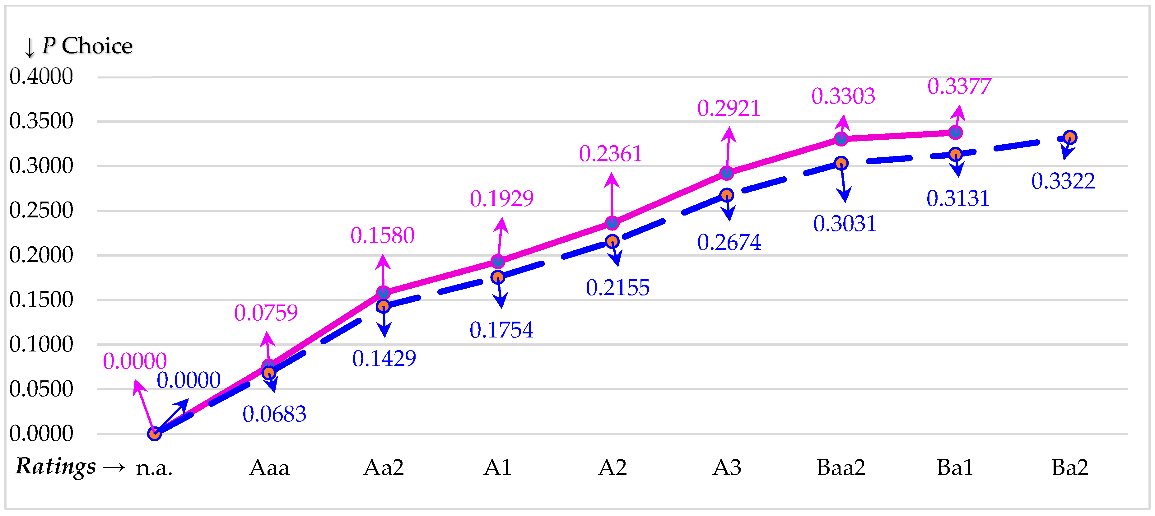
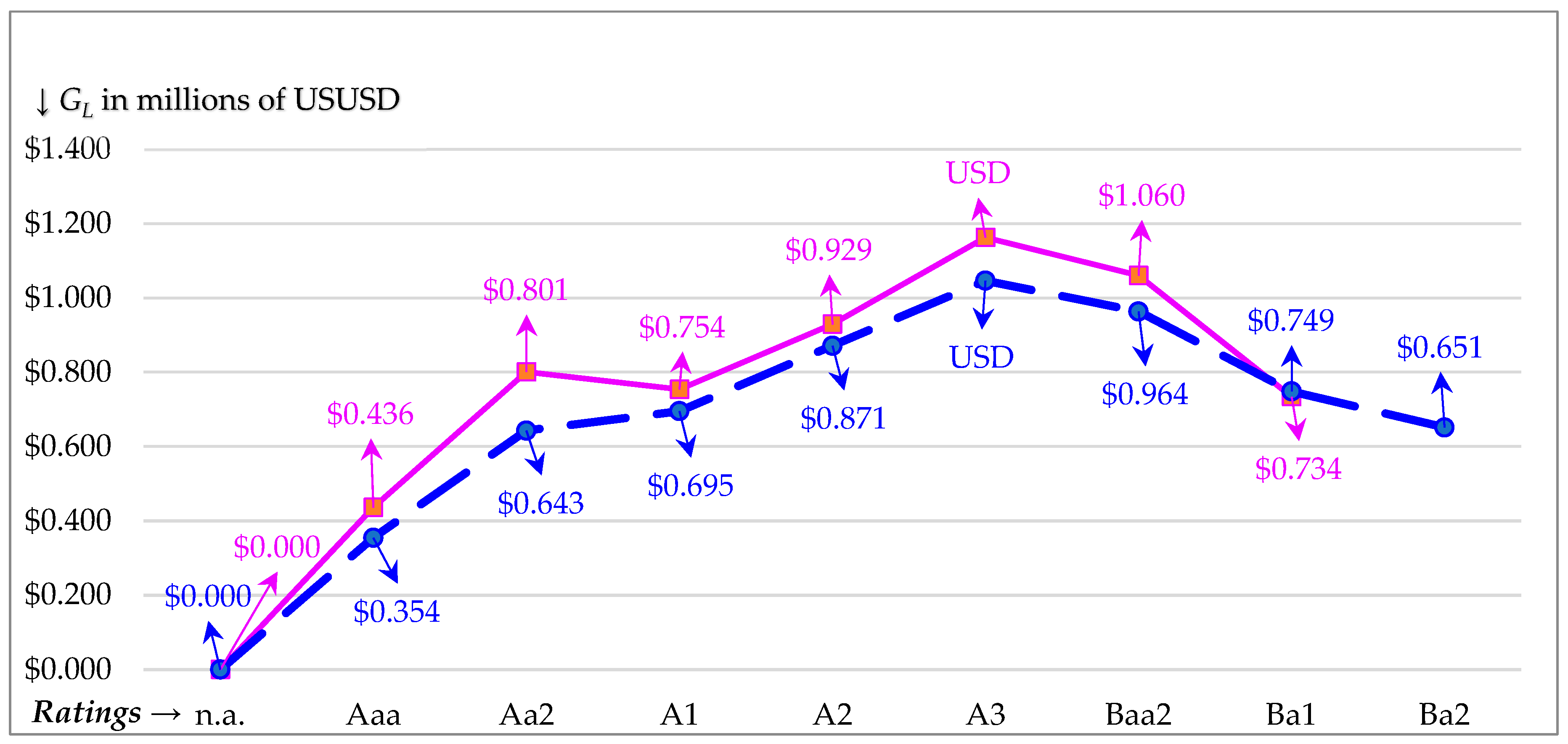
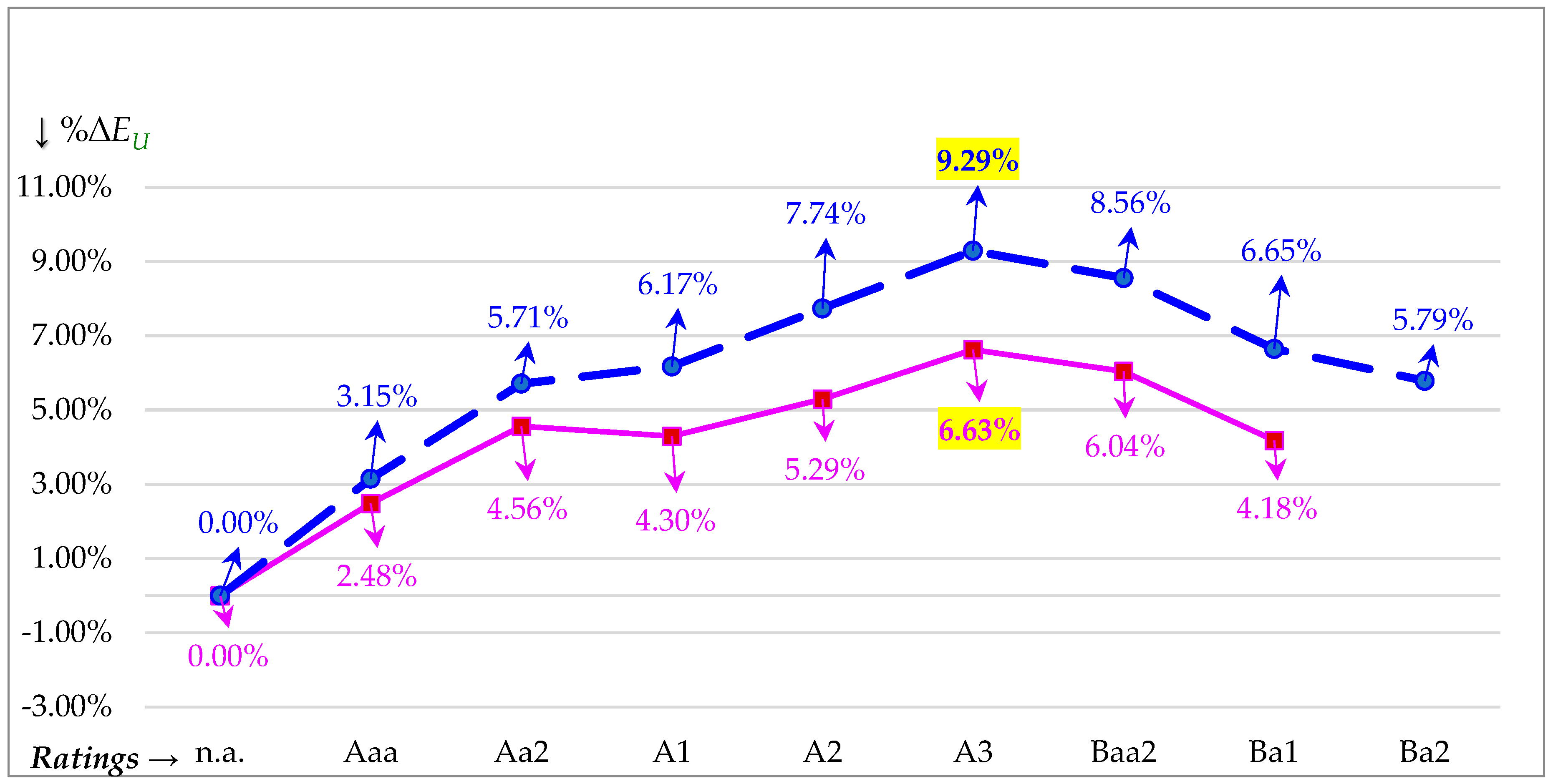
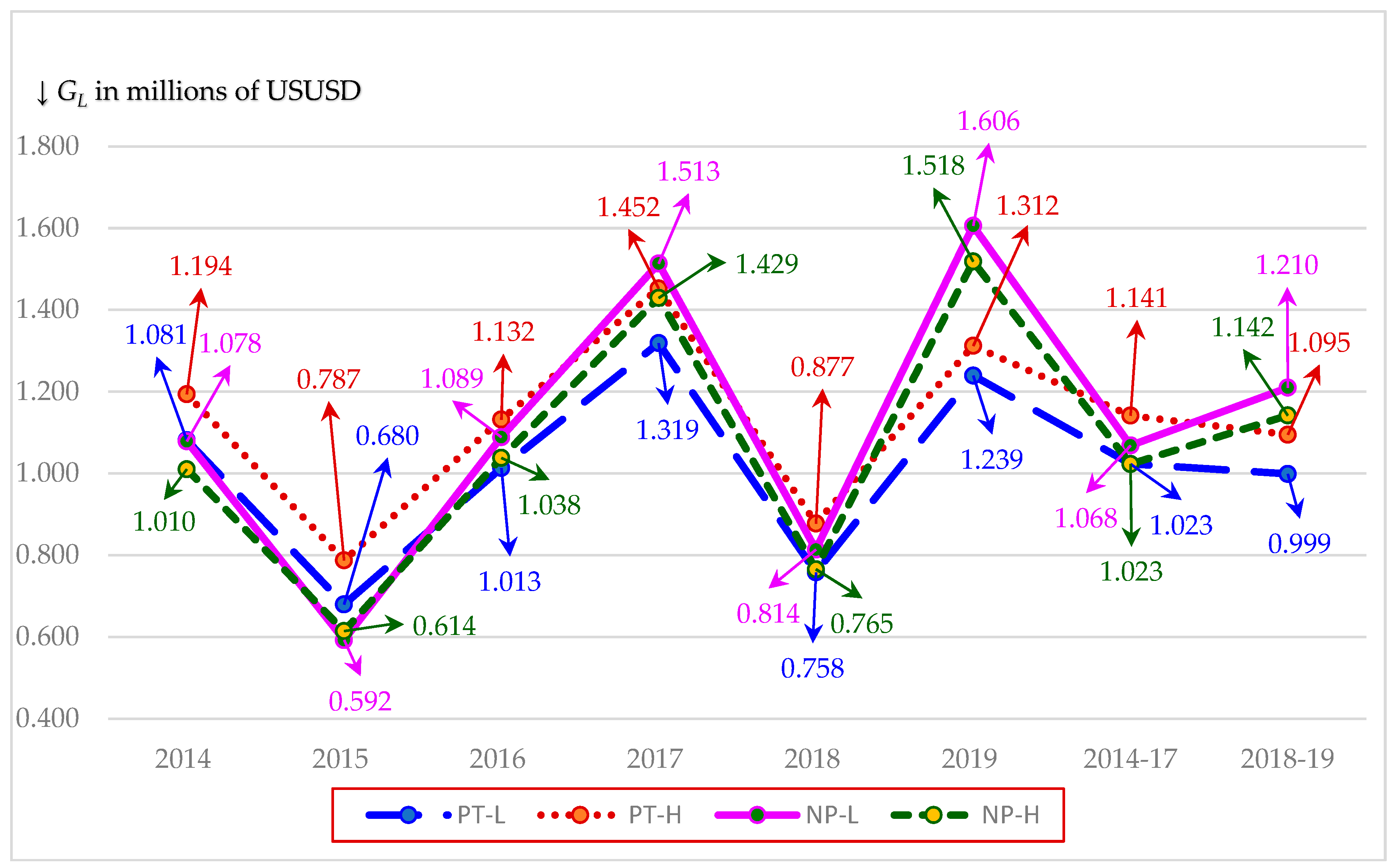
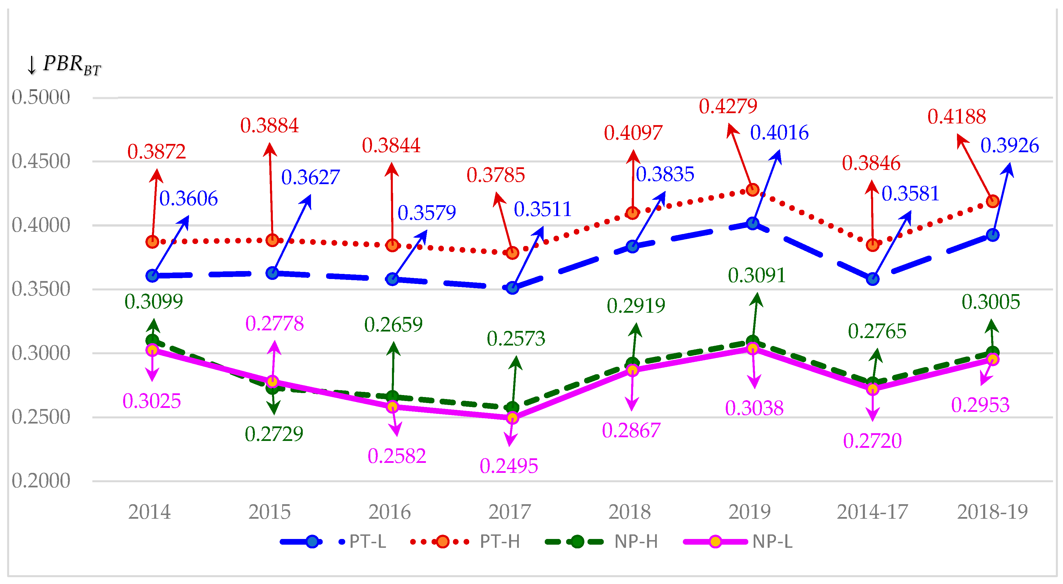
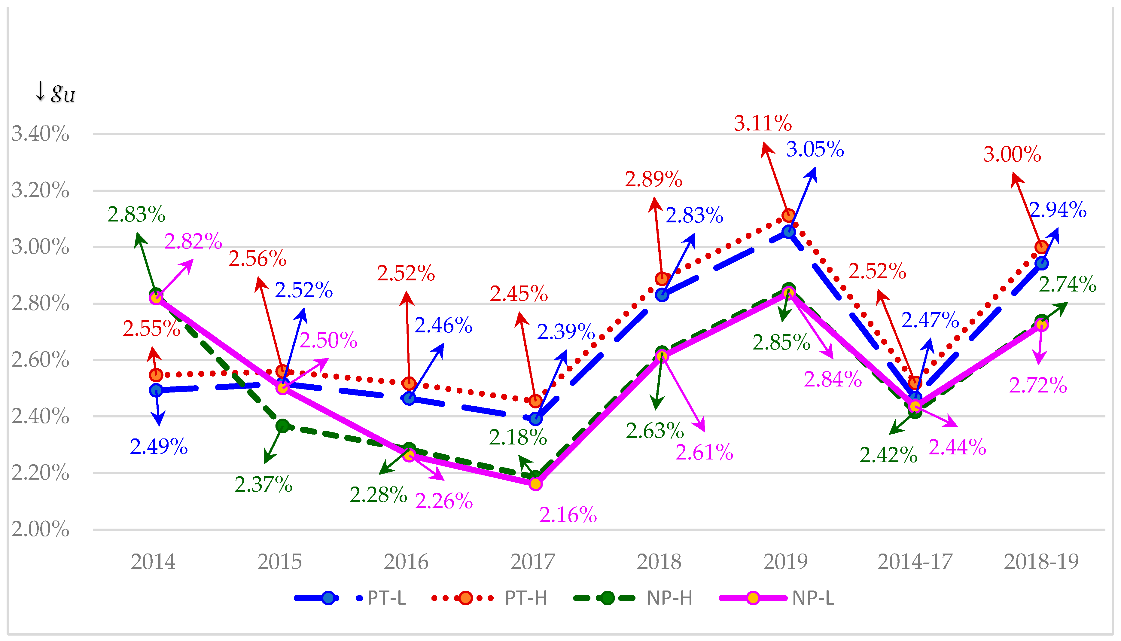
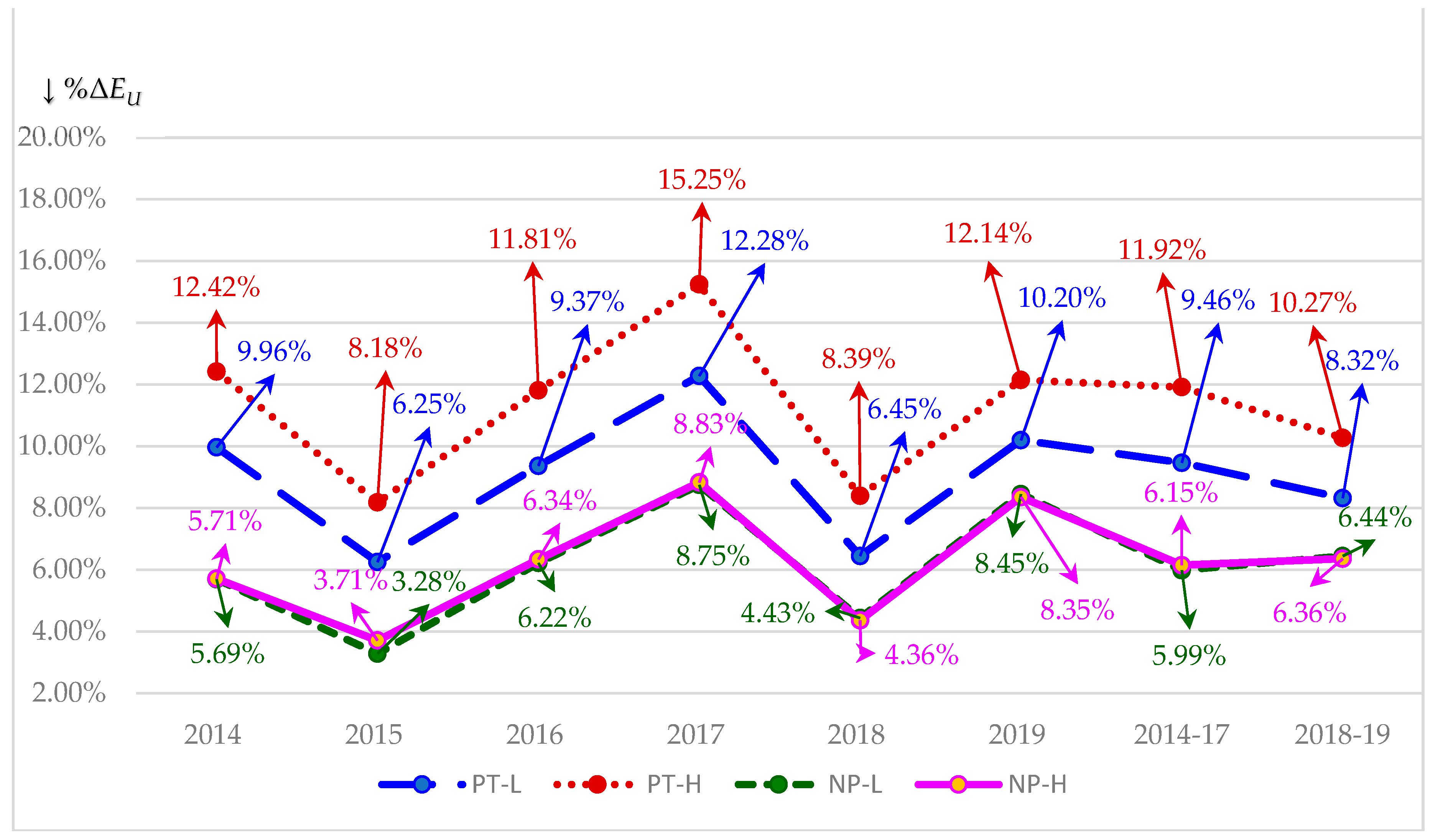
Table 1.
Costs of Borrowing.
| P Choice | ICR | Moody’s Rating | Credit Spread | rD | rL | βD | βL |
|---|---|---|---|---|---|---|---|
| 0.0759 | 24.000 | Aaa | 0.6300% | 3.1300% | 6.5800% | 0.1260 | 0.8160 |
| 0.1580 | 11.000 | Aa2 | 0.7800% | 3.2800% | 6.7300% | 0.1560 | 0.8460 |
| 0.1929 | 8.500 | A1 | 0.9750% | 3.4750% | 6.9250% | 0.1950 | 0.8850 |
| 0.2361 | 6.750 | A2 | 1.0764% | 3.5764% | 7.0264% | 0.2153 | 0.9053 |
| 0.2921 | 5.250 | A3 | 1.2168% | 3.7168% | 7.1668% | 0.2434 | 0.9334 |
| 0.3303 | 4.250 | Baa2 | 1.5600% | 4.0600% | 7.5100% | 0.3120 | 1.0020 |
| 0.3370 | 3.750 | Ba1 | 2.0000% | 4.5000% | 7.9500% | 0.4000 | 1.0900 |
| 0.3579 | 3.250 | Ba2 | 2.4000% | 4.9000% | 8.3500% | 0.4800 | 1.1700 |
| 0.3448 | 2.750 | B1 | 3.5100% | 6.0100% | 9.4600% | 0.7020 | 1.3920 |
| 0.3774 | 2.250 | B2 | 4.2120% | 6.7120% | 10.1620% | 0.8424 | 1.5324 |
| 0.4258 | 1.750 | B3 | 5.1480% | 7.6480% | 11.0980% | 1.0296 | 1.7296 |
| 0.3874 | 1.375 | Caa | 8.2000% | 10.7000% | 14.1500% | 1.6400 | 2.3300 |
| 0.4994 | 1.025 | Ca2 | 8.6424% | 11.1424% | 14.5924% | 1.7285 | 2.4185 |
| 0.6335 | 0.650 | C2 | 11.3412% | 13.8412% | 17.2912% | 2.2682 | 2.9582 |
| 0.8541 | 0.380 | D2 | 15.1164% | 17.6164% | 21.0664% | 3.0233 | 3.7133 |
Table 1 shows the process to compute P choices, costs of borrowing, and betas for the year 2019 using low (L) tax rates for nonprofit (NPs) under the Tax Cuts and Jobs Act (TCJA) where NP tax rates are zero as shown in Panel A of Exhibit 2. This process begins with retrieving credit spreads corresponding to fifteen credit ratings from Damodaran (2020) for the year 2019. Damodaran also supplies ranges for interest coverage ratios (ICRs) matched to spreads and ratings. These ranges are given for large, small, and financial service firms. We use the small ICRs as most NPs and pass-throughs (PTs) are small compared to C corps (CCs) for which large ICRs would be a better fit. We compute the average of the fifteen small ICR ranges as first described by Hull (2020a). The fifteen ICRs are given in the second column. Using Damodaran’s definition for ICR, Hull shows that interest (I) is computed as I = (1 − TC2)CFBT/ICR where TC2 is the effective (average) corporate tax rate on business income and CFBT is the before-tax cash flows that for our tests equals USD 1,000,000 (with CFBT analogous to EBIT). For PTs, the business tax rate is the levered personal tax rate (TE2). From the fifteen ICR values, we compute fifteen I values. From these fifteen I values, we use their corresponding levered personal debt rate (TD2) and cost of debt (rD) values to calculate fifteen debt (D) values where D = (1 − TD2)I/rD. We next compute the fifteen P choices where P is the proportion of unlevered equity (EU) retired by D. In equation form, we have P = D/EU. This table reports P choices for NPs in the first column along with corresponding Moody’s ratings and credit spreads in the third and fourth columns. As NPs and PTs have different TD2 values, the P choices provided in this table for NPs are not the same as those used for PTs. To get fifteen rD values (as seen in the rD column) we add each credit spread (CS) to the risk-free rate (rF) of 2.5% so that we have: rD = rF + CS. If we factor in the recent downward trend, an rF of 2.5% is consistent with the 30-year government bonds as given by Federal Reserve Economic Data (2020) for the past fifteen years. To get a cost of levered equity (rL) matched to each rD, we add an equity risk premium over a corporate bond portfolio (EPB) to each rD. Following Hull, we use EPB = 3.45%. By adding 3.45% to our fifteen increasing rD values, we get fifteen increasing rL values. In equation form, we have: rL = rD + EPB. From each rD and rL we compute respective debt beta (βD) and levered equity beta (βL) using the CAPM where βD = (rD − rF)/(rM − rF) and βL = (rL − rF)/(rM − rF).
Table 2.
Introductory Variables and Computations.
| Panel A. Alpha Computations |
| Nonprofit (NP) Alpha Computations: |
| For our L tax rate tests for NPs, α1 = α2 = 1 for all P choices because these tests assume NP tax rates are all zero. To illustrate with TE1 = TE2 = 0; TC1 = TC2 = 0; TD1 = TD2 = 0, we have: α1 = (1 − TE2)/(1 − TD2) = (1 − 0)(1 − 0)/(1 − 0) = 1.00. α2 = (1 − TE1)/(1 − TE2) = (1 − 0)/(1 − 0) = 1.00. |
| Pass-Through (PT) Alpha Computations: |
| The unlevered personal debt tax rate (TD1) only exist hypothetically for an unlevered situation, which is a way of saying we assign a beginning value to achieved an effective levered personal tax rate on debt (TD2) at the optimal P choice. For an unlevered situation, the unlevered personal equity tax rate (TE1) is 0.3, TD1 = 0.18, and the unlevered corporate tax rate (TC1) = 0. The latter is zero because PTs do not pay corporate taxes. For a levered situation, levered personal equity tax rate (TE2) is less than TE1 since TE2 decreases by 0.03 with each increasing P choice. TD2 is greater than TD1 since TD2 increases by 0.03 with each increasing P choice. For the first debt-for-equity choice using TE1 = 0.3, TD2 = TD1(1 + ΔTD1) = 0.18(1 + 0.03) = 0.1854, and TE2 = TE2(1 − ΔTE2) = 0.3(1 − 0.03) = 0.291, we have (to ten digits so later computations can minimize rounding off errors): α1 = (1 − TE2)/(1 − TD2) = (1 − 0.291)/(1 − 0.1854) = 0.8703658237. α2 = (1 − TE2)/(1 − TE1) = (1 − 0.291) (1 − 0.3) = 1.0128571429. For the fifth debt-for-equity choice using TD2 = TD1(1 + 0.03)5 = 0.18(1.1592740743) = 0.2086693 and TE2 = TE1(1 − 0.03)5 = 0.3(0.8587340257) = 0.25762021, we have: α1 = (1 − TE2)/(1 − TD2) = (1 − 0.25762021)/(1 − 0.2086693) = 0.9381410624. α2 = (1 − TE2)/(1 − TE1) = (1 − 0.25762021)/(1 − 0.3) = 1.0605425604. |
| Panel B. Unlevered Firm Value (EU) Computations |
| NP example using CC definitions given in Section 3.1: PBRBT = 0.2598; CFBT = USD 1,000,000; RE = PBRBT(CFBT) = 0.2598(USD 1,000,000) = USD 259,800. Cost to use RE (CRE) = TC2(RE) = 0(USD 259,800) = USD 0. %CRE per USD 1,000,000 of CFBT = USD 0/USD 1,000,000 = 0.00 or 0%. C = (1 − PBRBT)(CFBT) = (1 − 0.2598)(USD 1,000,000) = USD 740,200. gU = rU(1 − TC1)RE/C = 0.065(1 − 0)USD 259,800/USD 740,200 = 2.28141043%. EU = (1 − PBRBT)(1 − TE1)(1 − TC1)CFBT/(rU − gU) = (1 − 0.2598)(1 − 0)(1 − 0)USD 1,000,000/(0.065 − 0.0228141043) = USD 17,546,149. |
| PT example using PT definitions given in Section 3.1: PBRBT = 0.3519; CFBT = USD 1,000,000; RE = PBRBT(CFBT) = 0.3519(USD 1,000,000) = USD 351,900. Cost to use RE (CRE) = TE2(RE) = 0.25762021(USD 259,800) = USD 90,657. %CRE per USD 1,000,000 of CFBT = USD 90,657/USD 1,000,000 = 0.090657 or about 9.07%. C = (1 − PBRBT)(CFBT) = (1 − 0.3519)(USD 1,000,000) = USD 648,100. gU = rU(1 − TE1)RE/C = 0.065(1 − 0.3)USD 351,900/USD 648,100 = 0.0247052152 or 2.47052152%. EU = (1 − PBRBT)(1 − TE1)CFBT/(rU − gU) = (1 − 0.3519)(1 − 0.3)USD 1,000,000/(0.065 − 0.0247052152) = USD 11,258,777. |
Panel A provides NP and PT examples for computing the two alpha coefficients (α1 and α2) presented in Section 3.1. These coefficients capture the impact of tax rates in GL equations. This panel provides sample computations for α1 and α2 for the two ownership categories of nonprofits (NPs) and pass-throughs (PTs). For the illustration in this table, we use the low (L) tax rates under TCJA from the bottom half of Panel A in Exhibit 2. The values for α1 and α2 rise for increasing P choices as long as at least one tax rate is positive. For our tests, positive tax rates change by 0.03 for each subsequent P in the directions discussed by Hull (2014) as described in Section 2.3. For NPs, α1 and α2 do not change for L tax rate tests because all tax rates are zero. The latter is seen below. Panel B provides NP and PT examples for computing the unlevered firm value (EU). EU is important since each debt choice retires a fraction of EU. Consistent with Damodaran (2020), we use 7.5% for the market return (rM) and 0.8000 for the unlevered equity beta (βU). Given these values and rF = 2.50 from Table 1, the unlevered equity rate of return (rU) given by the CAPM is rU = rF + βU(rM − rF) = 2.5% + 0.8000(7.5% − 2.5%) = 6.50%. When applying the CSM with growth, the before-tax plowback ratio (PBRBT) is set by trial and error until gL = 3.12% is achieved at the optimal credit rating (OCR) where the latter is determined by the nongrowth test as described in Section 3.2.
Table 3.
Nonprofit Illustration.
| Panel A. Key Outcomes for P Choices (Optimal Outcomes in Bold Print) | |||||||||
| P Choice = Proportion of Unlevered Firm Value (EU) Retired by Debt (D) | |||||||||
| Outcomes | 0.0000 | 0.0759 | 0.1580 | 0.1929 | 0.2361 | 0.2921 | 0.3303 | 0.3377 | 0.3579 |
| Moody’s Rating | n.a. | Aaa | Aa2 | A1 | A2 | A3 | Baa2 | Ba1 | Ba2 |
| Debt (D) | 0.000 | 1.331 | 2.772 | 3.386 | 4.42 | 5.125 | 5.795 | 5.926 | n.a. |
| Equity growth rate: gL | 2.28% | 2.38% | 2.56% | 2.75% | 2.90% | 3.12% | 3.57% | 4.12% | n.a. |
| 1st component of GL | 0.000 | 0.338 | 0.591 | 0.567 | 0.556 | 0.418 | −0.175 | −1.031 | n.a. |
| 2nd component of GL | 0.000 | 0.098 | 0.210 | 0.187 | 0.373 | 0.745 | 1.235 | 1.765 | n.a. |
| Gain to leverage: GL | 0.000 | 0.436 | 0.801 | 0.754 | 0.929 | 1.163 | 1.060 | 0.734 | n.a. |
| Firm value: VL | 17.546 | 17.982 | 18.347 | 18.300 | 18.475 | 18.709 | 18.607 | 18.280 | n.a. |
| Equity value: EL | 17.546 | 16.651 | 15.575 | 14.914 | 14.333 | 13.584 | 12.811 | 12.354 | n.a. |
| %∆EU | 0.00% | 2.48% | 4.56% | 4.30% | 5.29% | 6.63% | 6.04% | 4.18% | n.a. |
| NB | 0.00% | 32.74% | 28.88% | 22.27% | 22.42% | 22.69% | 18.30% | 12.39% | n.a. |
| DV | 0.0000 | 0.0740 | 0.1511 | 0.1850 | 0.2242 | 0.2739 | 0.3115 | 0.3242 | n.a. |
| Panel B. Computations for Optimal Outcomes at P = 0.2921 | |||||||||
| D = P = 0.2921(USD 17,546,148.72) = USD 5,124,736.08 or D = (1 − TD2)I/rD = (1 − 0)USD 190,476.19/0.037168 = USD 5,124,736.08. gL = rL(1 − TC2)RE/[C + G − (1 − TC2)I] = 0.71668(1 − 0)USD 259,800/[USD 740,200 + USD 47,052.52 − (1 − 0)USD 190,476.19] = 0.0311998742 or about 3.12%. Max GL = (1 − αIrD/rLg)D + (1 − α2rUg/rLg)EU = [1 − 1.00000(0.037168)/0.0404681258]USD 5,124,736.08 + [1 − 1.00(0.0421858957)/0.0404681258]USD 17,546,148.72 = USD 417,915.91 − USD 744,789.77 = USD 1,162,706. Max VL = EU + Max GL = USD 17,546,149 + USD 1,162,706 = USD 18,708,854. EL = VL − D = USD 18,708,854 − USD 5,124,736.08 = USD 13,584,118. Max %∆EU = Max GL/EU = USD 1,162,706/USD 17,546,149 = 0.0663 or 6.63%. NB = Max GL/D = USD 1,162,706/USD 5,124,736.08 = 0.2269 or 22.69%. ODV = D/Max VL = USD 5,124,736.08/USD 18,708,854 = 0.2739. | |||||||||
Panel A uses Equation (2) to provide outcomes for the unlevered P choice and the seven feasible levered P choices for a nonprofit (NP) where P is the proportion of unlevered equity (EU) retired by debt (D). This table uses 2019 data (including spreads) from Damodaran (2020). In the last column, n.a. stands for not applicable as the growth (RE) constraint is violated once P reaches 0.3579. Violations of the growth constraint are described in Section 3.1. When using equation (2), we follow Hull (2014) and allow positive tax rates to change as described in Section 2.3. However, this table uses NP low (L) tax rates for TCJA tests that are all zero and so cannot change as the P choice changes. These zero tax rates are given in the nonprofit column of the bottom half of Panel A in Exhibit 2. As tax rates are all zero, α1 and α2 equal one as described in Table 2. Outcomes are based on before-tax cash flows (CFBT) of USD 1,000,000 with a historical growth rate of 3.12% that is achieved when a Moody’s A3 is the optimal credit rating (OCR). OCR is determined by the nongrowth test described in Section 3.2. Dollar values for key outcomes are in millions and are after-tax values. Firm value (VL) = EU + gain to leverage (GL). Levered equity (EL) = VL − D. %∆EU is GL as a percent of EU. Net benefit from leverage (NB) is GL as a percent of D. DV is the debt-to-firm value ratio. The optimal DV is ODV and is identified from the maximum gain to leverage (max GL) that coincides with the maximum firm value (max VL) since max VL = EU + max GL. Optimal outcomes are designated by the bold print column where the optimal P = 0.2921. Panel B provides computation for the optimal outcomes. Panel B computes outcomes at ODV as designated in the bold print column. To minimize rounding off errors, we use values up to eleven decimal points. From Table 1, we have ICR = 5.25, rD = 3.7168% and rL = 7.1668% when Moody’s rating is A3, which is the OCR. From Table 2, we have TE1 = TE2 = TD1 = TD2 = TC1 = TC2 = 0, gU = 2.28141043%, rU = 6.5%, CFBT = USD 1,000,000, RE = USD 259,800, C = USD 740,200, EU (or VU) = USD 17,546,149 and the before-tax plowback ratio (PBRBT) = 0.2598. For the optimal choice of P = 0.2921 where debt retires 0.2921 of EU, and I = (1 − TC2)CFBT/ICR = (1−0)USD 1,000,000/5.25 = USD 190,476.19, we compute D. Given G (as determined by iterative process due G’s interdependence with GL and gL) = rLgGL /(1 − TE2)(1 − TC2) = 0.0404681258(USD 1,162,705.69)/(1 − 0)(1 − 0) = USD 47,052.52, we compute gL. Using Equation (2) with α1 = 1.00 α2 = 1.00, rUg = rU − gU = 6.5% − 2.28141043% = 4.21858957%, rLg = rL − gL = 7.1668% − 3.11998742% = 4.04681258%, and above values for EU, rD, and D, we compute Max GL.
Table 4.
Pass-Through Illustration.
| Panel A. Key Outcomes for P Choices (Optimal Outcomes in Bold Print) | |||||||||
| P Choice = Proportion of Unlevered Firm Value (EU) Retired by Debt (D) | |||||||||
| Outcomes | 0.0000 | 0.0683 | 0.1429 | 0.1754 | 0.2155 | 0.2674 | 0.3031 | 0.3131 | 0.3322 |
| Moody’s Rating | n.a. | Aaa | Aa2 | A1 | A2 | A3 | Baa2 | Ba1 | Ba2 |
| Debt (D) | 0.000 | 0.769 | 1.609 | 1.975 | 2.426 | 3.011 | 3.413 | 3.525 | 3.740 |
| Equity growth rate: gL | 2.47% | 2.54% | 2.67% | 2.83% | 2.94% | 3.12% | 3.49% | 3.97% | 4.49% |
| 1st component of GL | 0.000 | 0.251 | 0.457 | 0.460 | 0.468 | 0.417 | 0.116 | −0.317 | −0.919 |
| 2nd component of GL | 0.000 | 0.104 | 0.186 | 0.235 | 0.403 | 0.629 | 0.848 | 1.066 | 1.570 |
| Gain to leverage: GL | 0.000 | 0.354 | 0.643 | 0.695 | 0.871 | 1.046 | 0.964 | 0.749 | 0.651 |
| Firm value: VL | 11.259 | 11.613 | 11.902 | 11.954 | 12.130 | 12.305 | 12.222 | 12.007 | 11.910 |
| Equity value: EL | 11.259 | 10.844 | 10.292 | 9.979 | 9.704 | 9.294 | 8.810 | 8.483 | 8.170 |
| %∆EU | 0.00% | 3.15% | 5.71% | 6.17% | 7.74% | 9.29% | 8.56% | 6.65% | 5.79% |
| NB | 0.00% | 46.11% | 39.96% | 35.20% | 35.91% | 34.75% | 28.23% | 21.24% | 17.42% |
| DV | 0.0000 | 0.0662 | 0.1352 | 0.1652 | 0.2000 | 0.2447 | 0.2792 | 0.2935 | 0.3140 |
| Panel B. Computations for Optimal Outcomes at P = 0.2674 | |||||||||
| D = P(EU) = 0.2674(USD 11,258,777.1) = USD 3,010,617.92 or D = (1 − TD2)I/rD = (1 − 0.208669333)USD 141,405.67/0.037168 = USD 3,010,617.92. gL = rL(1 − TC2)RE/[C + G − (1 − TC2)I] = 0.071668(1 − 0.25762021)USD 351,900/[USD 648,100 + USD 57,036.74 − (1 − 0.25762021)USD 141,405.67] = 0.0311963388 or about 3.12%. Max GL = (1 − αIrD/rLg)D + (1 − α2rUg/rLg)EU = [1 − 0.9381410624(0.037168)/0.04029478476]USD 3,010,617.92 + [1 − 1.0605425604(0.04029478476)/0.0404716612]USD 11,258,777.1 = USD 416,785 − USD 629,451 = USD 1,046,236. Max VL = EU + Max GL = USD 11,258,777 + USD 1,046,236 = USD 12,305,013. EL = VL − D = USD 12,305,013 − USD 3,010,617.92 = USD 9,294,396. Max %∆EU = Max GL/EU = USD 1,046,236/USD 11,258,777 = 0.0929 or 9.29%. NB = Max GL/D = USD 1,046,236/USD 3,010,617.92 = 0.3475 or 34.75%. ODV = D/Max VL = USD 3,010,617.92/USD 12,305,013 = 0.2447. | |||||||||
Panel A uses equation (4) to provide outcomes for the unlevered P choice and eight feasible levered P choices for a pass-through (PT) where P is the proportion of unlevered equity (EU) retired by debt (D). This table uses 2019 data (including spreads) from Damodaran (2020). Violations of the growth (RE) constraint, described in Section 3.1, do not hold for this table as the first violation does not occur until the ninth levered P choice. When using Equation (4), we follow Hull (2014) and allow tax rates to be a function of debt causing α1 and α2 to increase as debt rises as described in Section 2.3. This table uses the low (L) tax rates under TCJA in the PT column in the bottom half of Panel A in Exhibit 2. Outcomes are based on before-tax cash flows (CFBT) of USD 1,000,000 with a historical growth rate of 3.12% that is achieved when a Moody’s A3 is the optimal credit rating (OCR). OCR is determined by the nongrowth test described in Section 3.2. Dollar values are in millions and are after-tax values. Firm value (VL) = EU + gain to leverage (GL). Levered equity (EL) = VL − D. %∆EU is GL as a percent of EU. Net benefit from leverage (NB) is GL as a percent of D. DV is the debt-to-firm value ratio. The optimal DV is ODV and is identified from the maximum gain to leverage (max GL) that coincides with the maximum firm value (max VL) since max VL = EU + max GL. Optimal outcomes are designated by the bold print column where the optimal P = 0.2674. Panel B computes outcomes at ODV as designated in the bold print column. To minimize rounding off errors, we use values up to eleven decimal points. From Table 1, we have ICR = 5.25, rD = 3.7168% and rL = 7.1668% when Moody’s rating is A3, which is the OCR. From Table 2, we have TE1 = 0.30, TE2 = 0.25762021, TD2 = 0.208669333, gU = 2.47052152%, rU = 6.5%, CFBT = USD 1,000,000, RE = USD 351,900, C = USD 648,100, EU (or VU) = USD 11,258,777 and the before-tax plowback ratio (PBRBT) = 0.3519. For the optimal choice of P = 0.2674 where debt retires 0.2674 of EU, and I = (1 − TE2)CFBT/ICR = (1 − 0.25762021) USD 1,000,000/5.25 = USD 141,405.67, we compute D. Given G (as determined by iterative process due G’s interdependence with GL and gL) = rLgGL / (1 − TE2) = 0.040471661199 (USD 1,046,236.37) / (1 − 0.2576202077) = USD 57,036.74, we compute gL. Using Equation (4) with α1 = 0.9381410624, α2 = 1.0605425604, rUg = rU − gU = 6.5% − 2.47052152% = 4.029478476%, rLg = rL − gL = 7.1668% − 3.11963388% = 4.0471661199%, and above values for EU, rD, and D, we compute Max GL.
Table 5.
Optimal Outcomes for NPs and PTs.
| P | PBRBT | gU | EU | Max VL | Max GL | Max %∆EU | NB | ODV | OCR | DGN | |
|---|---|---|---|---|---|---|---|---|---|---|---|
| 2014: NP-L | 0.1499 | 0.3025 | 2.819% | USD 18.949 | USD 20.027 | USD 1.078 | 5.69% | 37.96% | 0.1419 | Aa2 | USD 3.516 |
| 2014: NP-H | 0.1474 | 0.3073 | 2.826% | USD 18.107 | USD 19.129 | USD 1.022 | 5.64% | 38.27% | 0.1395 | Aa2 | USD 3.274 |
| 2014: PT-L | 0.2683 | 0.3528 | 2.480% | USD 11.270 | USD 12.340 | USD 1.070 | 9.49% | 35.38% | 0.2451 | A3 | USD 0.401 |
| 2014: PT- H | 0.2806 | 0.3786 | 2.535% | USD 10.029 | USD 11.211 | USD 1.182 | 11.78% | 41.99% | 0.2510 | A3 | USD 0.006 |
| 2015: NP-L | 0.1810 | 0.2778 | 2.500% | USD 18.056 | USD 18.649 | USD 0.592 | 3.28% | 18.18% | 0.1752 | A1 | USD 2.865 |
| 2015: NP-H | 0.1777 | 0.2826 | 2.509% | USD 17.265 | USD 17.828 | USD 0.563 | 3.26% | 18.36% | 0.1721 | A1 | USD 2.668 |
| 2015: PT-L | 0.2047 | 0.3551 | 2.505% | USD 11.301 | USD 11.964 | USD 0.663 | 5.86% | 28.65% | 0.1934 | A2 | USD 0.560 |
| 2015: PT- H | 0.2137 | 0.3800 | 2.550% | USD 10.045 | USD 10.815 | USD 0.770 | 7.67% | 35.88% | 0.1985 | A2 | USD 0.161 |
| 2016: NP-L | 0.2902 | 0.2582 | 2.262% | USD 17.505 | USD 18.594 | USD 1.089 | 6.22% | 21.43% | 0.2732 | A3 | USD 2.271 |
| 2016: NP-H | 0.2843 | 0.2630 | 2.273% | USD 16.746 | USD 17.776 | USD 1.031 | 6.15% | 21.65% | 0.2678 | A3 | USD 2.111 |
| 2016: PT-L | 0.2656 | 0.3501 | 2.451% | USD 11.236 | USD 12.235 | USD 1.000 | 8.90% | 33.50% | 0.2439 | A3 | USD 0.399 |
| 2016: PT- H | 0.2777 | 0.3759 | 2.506% | USD 10.000 | USD 11.117 | USD 1.118 | 11.18% | 40.25% | 0.2498 | A3 | USD 0.008 |
| 2017: NP-L | 0.3608 | 0.2495 | 2.161% | USD 17.296 | USD 18.809 | USD 1.513 | 8.75% | 24.25% | 0.3318 | Baa2 | USD 1.977 |
| 2017: NP-H | 0.3531 | 0.2543 | 2.172% | USD 16.549 | USD 17.975 | USD 1.426 | 8.62% | 24.40% | 0.3251 | Baa2 | USD 1.836 |
| 2017: PT-L | 0.3295 | 0.3433 | 2.379% | USD 11.154 | USD 12.462 | USD 1.308 | 11.73% | 35.60% | 0.2949 | Baa2 | USD 0.231 |
| 2017: PT- H | 0.3452 | 0.3698 | 2.441% | USD 9.937 | USD 11.378 | USD 1.441 | 14.50% | 42.00% | 0.3015 | Baa2 | −USD 0.152 |
| 2018: NP-L | 0.2733 | 0.2431 | 2.088% | USD 17.154 | USD 17.584 | USD 0.430 | 2.51% | 9.18% | 0.2666 | A3 | USD 2.120 |
| 2018: NP-H | 0.2677 | 0.2479 | 2.100% | USD 16.415 | USD 16.819 | USD 0.404 | 2.46% | 9.20% | 0.2613 | A3 | USD 1.974 |
| 2018: PT-L | 0.2493 | 0.3335 | 2.277% | USD 11.047 | USD 11.630 | USD 0.583 | 5.28% | 21.18% | 0.2368 | A3 | USD 0.391 |
| 2018: PT- H | 0.2606 | 0.3590 | 2.330% | USD 9.838 | USD 10.576 | USD 0.739 | 7.51% | 28.83% | 0.2424 | A3 | USD 0.027 |
| 2019: NP-L | 0.2921 | 0.2598 | 2.281% | USD 17.546 | USD 18.709 | USD 1.163 | 6.63% | 22.69% | 0.2739 | A3 | USD 2.289 |
| 2019: NP-H | 0.2861 | 0.2647 | 2.293% | USD 16.786 | USD 17.888 | USD 1.102 | 6.56% | 22.94% | 0.2685 | A3 | USD 2.130 |
| 2019: PT-L | 0.2674 | 0.3519 | 2.471% | USD 11.259 | USD 12.305 | USD 1.046 | 9.29% | 34.75% | 0.2447 | A3 | USD 0.401 |
| 2019: PT-H | 0.2796 | 0.3777 | 2.525% | USD 10.019 | USD 11.179 | USD 1.160 | 11.58% | 41.41% | 0.2506 | A3 | USD 0.006 |
| 2014-17: NP-L | 0.2455 | 0.2720 | 2.44% | USD 17.952 | USD 19.020 | USD 1.068 | 5.99% | 25.44% | 0.2305 | A2 | USD 2.657 |
| 2014-17: NP-H | 0.2406 | 0.2768 | 2.45% | USD 17.167 | USD 18.177 | USD 1.010 | 5.92% | 25.67% | 0.2261 | A2 | USD 2.472 |
| 2014-17: PT-L | 0.2670 | 0.3503 | 2.45% | USD 11.240 | USD 12.250 | USD 1.010 | 9.00% | 33.28% | 0.2443 | A3 | USD 0.398 |
| 2014-17: PT-H | 0.2793 | 0.3761 | 2.51% | USD 10.003 | USD 11.130 | USD 1.128 | 11.28% | 40.03% | 0.2502 | A3 | USD 0.006 |
| 2018-19: NP-L | 0.2827 | 0.2515 | 2.185% | USD 17.350 | USD 18.147 | USD 0.796 | 4.57% | 15.93% | 0.2703 | A3 | USD 2.204 |
| 2018-19: NP-H | 0.2769 | 0.2563 | 2.196% | USD 16.601 | USD 17.354 | USD 0.753 | 4.51% | 16.07% | 0.2649 | A3 | USD 2.052 |
| 2018-19: PT-L | 0.2584 | 0.3427 | 2.374% | USD 11.153 | USD 11.968 | USD 0.815 | 7.29% | 27.96% | 0.2407 | A3 | USD 0.396 |
| 2018-19: PT-H | 0.2701 | 0.3684 | 2.427% | USD 9.928 | USD 10.878 | USD 0.950 | 9.55% | 35.12% | 0.2465 | A3 | USD 0.017 |
Table 5 reports values for eleven outcomes for tests using a 3.12% growth rate and TCJA low (L) and TCJA high (H) tax rates given in Exhibit 2. The H results reported in this table supplement the L results that were the focus of Table 1, Table 2, Table 3 and Table 4 and Figure 1, Figure 2, Figure 3, Figure 4 and Figure 5. The first column designates the year or period, the ownership form (NP or PT), and the tax rate test (L or H) for the subsequent columns. The outcomes for the next ten columns were described earlier in Table 2, Table 3 and Table 4. The last column contains a new outcome that is labeled DGN, which refers to the difference of max VL with growth minus max VL with nongrowth. All dollar values are in millions. In order to report outcomes for years 2014–2017, we have to assume the same ICRs for these four years as given by Damodaran (2019, 2020) for 2018 and 2019 where these two years have ICRs that are the same. ICRs enable us to compute leverage ratios. The purpose of including the years 2014–2017 is not to report the most precise results (since we do not know the ICRs for these four years) but to illustrate how the eleven outcomes change when credit ratings change if ICRs are held constant using TCJA tax rates that began in 2018.
Table 6.
Optimal Outcomes for NPs and PTs with Adjustments for Pre-TCJA Tax Rates and TCJA Growth.
| P | PBRBT | gU | EU | Max VL | Max GL | Max %∆EU | NB | ODV | OCR | DGN | |
|---|---|---|---|---|---|---|---|---|---|---|---|
| 2014: NP-L | 0.1499 | 0.3025 | 2.819% | USD 18.949 | USD 20.027 | USD 1.078 | 5.69% | 37.96% | 0.1419 | Aa2 | USD 3.516 |
| 2014: NP-H | 0.1477 | 0.3099 | 2.831% | USD 17.699 | USD 18.709 | USD 1.010 | 5.71% | 38.64% | 0.1397 | Aa2 | USD 3.149 |
| 2014: PT-L | 0.2683 | 0.3606 | 2.493% | USD 10.850 | USD 11.931 | USD 1.081 | 9.96% | 37.14% | 0.2440 | A3 | USD 0.279 |
| 2014: PT- H | 0.2814 | 0.3872 | 2.546% | USD 9.610 | USD 10.803 | USD 1.194 | 12.42% | 44.14% | 0.2503 | A3 | −USD 0.114 |
| 2015: NP-L | 0.1810 | 0.2778 | 2.500% | USD 18.056 | USD 18.649 | USD 0.592 | 3.28% | 18.13% | 0.1752 | A1 | USD 2.865 |
| 2015: NP-H | 0.2193 | 0.2729 | 2.366% | USD 16.551 | USD 17.165 | USD 0.614 | 3.71% | 16.92% | 0.2114 | A2 | USD 2.273 |
| 2015: PT-L | 0.2047 | 0.3627 | 2.516% | USD 10.876 | USD 11.556 | USD 0.680 | 6.25% | 30.53% | 0.1926 | A2 | USD 0.433 |
| 2015: PT- H | 0.2142 | 0.3884 | 2.559% | USD 9.622 | USD 10.410 | USD 0.787 | 8.18% | 38.19% | 0.1980 | A2 | USD 0.038 |
| 2016: NP-L | 0.2902 | 0.2582 | 2.262% | USD 17.505 | USD 18.594 | USD 1.089 | 6.22% | 21.43% | 0.2732 | A3 | USD 2.271 |
| 2016: NP-H | 0.2846 | 0.2659 | 2.284% | USD 16.382 | USD 17.420 | USD 1.038 | 6.34% | 22.27% | 0.2676 | A3 | USD 2.022 |
| 2016: PT-L | 0.2655 | 0.3579 | 2.464% | USD 10.817 | USD 11.831 | USD 1.013 | 9.37% | 35.27% | 0.2428 | A3 | USD 0.277 |
| 2016: PT- H | 0.2785 | 0.3844 | 2.516% | USD 9.581 | USD 10.713 | USD 1.132 | 11.81% | 42.42% | 0.2491 | A3 | −USD 0.111 |
| 2017: NP-L | 0.3608 | 0.2495 | 2.161% | USD 17.296 | USD 18.809 | USD 1.513 | 8.75% | 24.25% | 0.3318 | Baa2 | USD 1.977 |
| 2017: NP-H | 0.3534 | 0.2573 | 2.184% | USD 16.192 | USD 17.621 | USD 1.429 | 8.83% | 24.98% | 0.3247 | Baa2 | USD 1.753 |
| 2017: PT-L | 0.3295 | 0.3511 | 2.392% | USD 10.740 | USD 12.059 | USD 1.319 | 12.28% | 37.26% | 0.2935 | Baa2 | USD 0.144 |
| 2017: PT- H | 0.3463 | 0.3785 | 2.454% | USD 9.524 | USD 10.977 | USD 1.452 | 15.25% | 44.04% | 0.3004 | Baa2 | −USD 0.265 |
| 2018: NP-L | 0.2555 | 0.2867 | 2.613% | USD 18.349 | USD 19.163 | USD 0.814 | 4.43% | 17.36% | 0.2447 | A3 | USD 3.698 |
| 2018: NP-H | 0.2503 | 0.2919 | 2.626% | USD 17.554 | USD 18.320 | USD 0.765 | 4.36% | 17.42% | 0.2399 | A3 | USD 3.474 |
| 2018: PT-L | 0.2342 | 0.3835 | 2.830% | USD 11.760 | USD 12.518 | USD 0.758 | 6.45% | 27.52% | 0.2200 | A3 | USD 1.279 |
| 2018: PT- H | 0.2451 | 0.4097 | 2.887% | USD 10.457 | USD 11.335 | USD 0.877 | 8.39% | 34.23% | 0.2261 | A3 | USD 0.785 |
| 2019: NP-L | 0.2697 | 0.3038 | 2.836% | USD 19.003 | USD 20.609 | USD 1.606 | 8.45% | 31.33% | 0.2487 | A3 | USD 4.189 |
| 2019: NP-H | 0.2642 | 0.3091 | 2.850% | USD 18.178 | USD 19.697 | USD 1.518 | 8.35% | 31.61% | 0.2439 | A3 | USD 3.939 |
| 2019: PT-L | 0.2477 | 0.4016 | 3.054% | USD 12.154 | USD 13.394 | USD 1.239 | 10.20% | 41.17% | 0.2248 | A3 | USD 1.489 |
| 2019: PT-H | 0.2593 | 0.4279 | 3.111% | USD 10.805 | USD 12.118 | USD 1.312 | 12.14% | 46.83% | 0.2312 | A3 | USD 0.945 |
| 2014-17: NP-L | 0.2259 | 0.2778 | 2.52% | USD 18.232 | USD 19.268 | USD 1.035 | 5.74% | 32.43% | 0.2121 | A2 | USD 2.657 |
| 2014-17: NP-H | 0.2320 | 0.2823 | 2.50% | USD 16.962 | USD 17.953 | USD 0.992 | 5.90% | 32.77% | 0.2178 | A2 | USD 2.299 |
| 2014-17: PT-L | 0.2670 | 0.3581 | 2.47% | USD 10.821 | USD 11.844 | USD 1.023 | 9.46% | 35.05% | 0.2432 | A3 | USD 0.276 |
| 2014-17: PT-H | 0.2801 | 0.3846 | 2.52% | USD 9.584 | USD 10.726 | USD 1.141 | 11.92% | 42.20% | 0.2495 | A3 | −USD 0.113 |
| 2018-19: NP-L | 0.2626 | 0.2953 | 2.724% | USD 18.676 | USD 19.886 | USD 1.210 | 6.44% | 24.34% | 0.2467 | A3 | USD 3.944 |
| 2018-19: NP-H | 0.2573 | 0.3005 | 2.738% | USD 17.866 | USD 19.008 | USD 1.142 | 6.36% | 24.52% | 0.2419 | A3 | USD 3.707 |
| 2018-19: PT-L | 0.2410 | 0.3926 | 2.942% | USD 11.957 | USD 12.956 | USD 0.999 | 8.32% | 34.34% | 0.2224 | A3 | USD 1.384 |
| 2018-19: PT-H | 0.2522 | 0.4188 | 2.999% | USD 10.631 | USD 11.726 | USD 1.095 | 10.27% | 40.53% | 0.2287 | A3 | USD 0.865 |
Table 6 repeats Table 5 with the following two adjustments. First, values for the years 2014 through 2017 use pre-TCJA tax rates given in Exhibit 2. Second, TCJA growth tests no longer use the historical growth rate of 3.12% but a higher rate of 3.90%. The rate of 3.12% is a rate suggested by annual U.S. real GDP growth rates as supplied by the U.S. Bureau of Economic Analysis (2018) the past seventy years. The rate of 3.90% assumes that lower taxes under TCJA will increase growth 0.78%. This increase of 0.78% is consistent with the Tax Policy Center (2018) that reports an estimated boost in growth per year of about 0.8% for both 2018–2020 (average of six sources) and for 2018–2027 (average of five sources). An increase of 0.78% added to 3.12% generates the 3.90% we use in this table for 2018 and 2019 TCJA tests.
Table 7.
NPs Versus PTs for the Period of 2018–2019.
| P | PBRBT | gU | EU | Max VL | Max GL | Max %∆EU | NB | ODV | OCR | DGN | |
|---|---|---|---|---|---|---|---|---|---|---|---|
| T5-L | 9.42% | −26.63% | −7.97% | 55.57% | 51.63% | −2.25% | −37.32% | −43.03% | 12.27% | A3 | USD 1.808 |
| T5-H | 2.53% | −30.42% | −9.52% | 67.20% | 59.53% | −20.69% | −52.72% | −54.24 | 7.47% | A3 | USD 2.035 |
| T6-L | 8.98% | −24.79% | −7.39% | 56.19% | 53.49% | 21.14% | −22.58% | −29.11% | 10.91% | A3 | USD 2.841 |
| T6-H | 2.01% | −28.25% | −8.72% | 68.05% | 62.10% | 4.30% | −38.09% | −39.52% | 5.77% | A3 | USD 2.841 |
| Mean | 5.73% | −27.52% | −8.40% | 61.75% | 56.69% | 0.62% | −37.68% | −41.48% | 9.10% | A3 | USD 2.311 |
| StDev | 4.01% | 2.39% | 0.92% | 6.80% | 4.94% | 17.29% | 12.31% | 10.36% | 3.00% | n.a. | USD 0.445 |
Table 7 presents percentage differences when comparing the NP and PT results in Table 5 (referred to as T5) and Table 6 (referred to as T6) for the four 2018–2019 tests of NP-L, NP-H, PT-L, and PT-H where the results for these 2018–2019 tests are found in the last four rows of Table 5 and Table 6. A positive percentage means that the NP value is greater than the PT value. The DGN column has just the difference in DGN values (NP value for DGN minus PT value for DGN) and not the percentage. DGN values are in millions. The last two rows have the mean and standard deviation (StDev) for the first four rows and n.a. stands for not applicable.
Exhibit 1.
Key Features of Nonprofits (NPs) and Pass-Throughs (PTs).
| Nonprofit | Pass-Through |
|---|---|
| Owned By: No one | Owned By: Investors |
| Ownership types: Corporation (501c3), association, trust | Ownership types: Sole proprietorship, partnership, LLC, S corp |
| Board Members: Nominated | Board Members: Elected by owners (if applicable) |
| Official obligations: Fulfill duties related to goals involving service, education, and research | Official obligations: Increase ownership wealth by providing profitable services and products |
| Major Goal: Maximize value in terms of service distributions | Major Goal: Maximize value in terms of monetary distributions |
| Mission: Described largely in terms of service, education, research, and growth | Mission: Described largely in terms of profit, efficiency, service, growth |
| Decision-making and implementation: Cautiously proceeds to satisfy mission and constituencies | Decision-making and implementation: Quickly responds to profitable opportunities |
| Sources of Revenues: Services, contributions, grants, and investments (including endowment income) | Sources of Revenues: Business activities (sales and services) and investments in other businesses |
| Equity Distributions: Non-monetary distributions in form of services rendered to those in need | Equity Distributions: Monetary distributions to owners in form of cash payouts and capital gains |
| Sources of Equity Financing: Internal equity (eligible revenues, investment/endowment income); External equity (contributions, grants, government) | Sources of Equity Financing: Internal equity (retained earnings); External equity (new partners, new issuances, venture capital) |
| Sources of Debt Financing: Personal tax-exempt debt, nonfinancial debt (mortgages), short-term debt (trade credit, bank borrowings avoided) | Sources of Debt Financing: Bond issues, mezzanine debt, Small Business Administration loans, short-term debt (trade credit, bank borrowings) |
| Corporate Taxes: Zero or very little taxes resulting from minor taxable profitable ventures | Corporate Taxes: None as PTs do not pay corporate taxes |
| Personal Equity Taxes: Zero or very little taxes from minor taxable for-profit ventures | Personal Equity Taxes: Personal taxes paid on business income (even if undistributed) |
| Personal Debt Taxes: Zero or minor due to issuing mostly tax-exempt debt | Personal Debt Taxes: Personal taxes paid on interest from debt |
| Interest Tax Shield: Zero or very little business tax shield (typically at corporate tax level) | Interest Tax Shield: Full business tax shield (at personal tax level) |
Exhibit 2.
Tax Rate Sets.
| Nonprofit (Unlevered and Levered Tax Rates) | Pass-Through (Unlevered and Levered Tax Rates) |
|---|---|
| Panel A: Low (L) Tax Rates | |
| Pre-TCJA | Pre-TCJA |
| TC1 = 0 and TC2 = 0 | TC1 = 0 and TC2 = 0 |
| TE1 = 0 and TE2 = 0 | TE1 = 0.320 and TE2 = 0.275 |
| TD1 = 0 and TD2 = 0 | TD1 = 0.190 and TD2 = 0.220 |
| TCJA | TCJA |
| TC1 = 0 and TC2 = 0 | TC1 = 0 and TC2 = 0 |
| TE1 = 0 and TE2 = 0 | TE1 = 0.300 and TE2 = 0.255 |
| TD1 = 0 and TD2 = 0 | TD1 = 0.180 and TD2 = 0.210 |
| Panel B: High (H) Tax Rates | |
| Pre-TCJA | Pre-TCJA |
| TC1 = 0.030 and TC2 = 0.025 | TC1 = 0 and TC2 = 0 |
| TE1 = 0.030 and TE2 = 0.025 | TE1 = 0.380 and TE2 = 0.330 |
| TD1 = 0.050 and TD2 = 0.060 | TD1 = 0.190 and TD2 = 0.220 |
| TCJA | TCJA |
| TC1 = 0.020 and TC2 = 0.020 | TC1 = 0 and TC2 = 0 |
| TE1 = 0.020 and TE2 = 0.020 | TE1 = 0.360 and TE2 = 0.310 |
| TD1 = 0.040 and TD2 = 0.045 | TD1 = 0.180 and TD2 = 0.210 |
Exhibit 3.
Credit Spreads: 2014 through 2019.
| Credit Ratings Moody’s/S&P | Credit Spreads by Years/Periods (Means for the Two Periods in the Last Two Columns) | |||||||
|---|---|---|---|---|---|---|---|---|
| 2014 | 2015 | 2016 | 2017 | 2018 | 2019 | 2014–2017 | 2018–2019 | |
| Aaa/AAA | 0.4000% | 0.7500% | 0.6000% | 0.5400% | 0.7500% | 0.6300% | 0.5725% | 0.6900% |
| Aa2/AA | 0.7000% | 1.0000% | 0.8000% | 0.7200% | 1.0000% | 0.7800% | 0.8050% | 0.8900% |
| A1/A+ | 0.9000% | 1.1000% | 1.0000% | 0.9000% | 1.2500% | 0.9750% | 0.9750% | 1.1125% |
| A2/A | 1.0000% | 1.2500% | 1.1000% | 0.9900% | 1.3750% | 1.0764% | 1.0850% | 1.2257% |
| A3/A- | 1.2000% | 1.7500% | 1.2500% | 1.1300% | 1.5625% | 1.2168% | 1.3325% | 1.3897% |
| Baa2/BBB | 1.7500% | 2.2500% | 1.6000% | 1.2700% | 2.0000% | 1.5600% | 1.7175% | 1.7800% |
| Ba1/BB+ | 2.7500% | 3.2500% | 2.5000% | 1.9800% | 3.0000% | 2.0000% | 2.6200% | 2.5000% |
| Ba2/BB | 3.2500% | 4.2500% | 3.0000% | 2.3800% | 3.6000% | 2.4000% | 3.2200% | 3.0000% |
| B1/B+ | 4.0000% | 5.5000% | 3.7500% | 2.9800% | 4.5000% | 3.5100% | 4.0575% | 4.0050% |
| B2/B | 5 0000% | 6.5000% | 4.5000% | 3.5700% | 5.4000% | 4.2120% | 4.8925% | 4.8060% |
| B3/B- | 6.0000% | 7.5000% | 5.5000% | 4.3700% | 6.6000% | 5.1480% | 5.8425% | 5.8740% |
| Caa/CCC | 7.0000% | 9.0000% | 6.5000% | 8.6400% | 9.0000% | 8.2000% | 7.7850% | 8.6000% |
| Ca2/CC | 8.0000% | 12.0000% | 8.0000% | 10.6300% | 11.0800% | 8.6424% | 9.6575% | 9.8612% |
| C2/C | 10.0000% | 16.0000% | 10.5000% | 13.9500% | 14.5400% | 11.3412% | 12.6125% | 12.9406% |
| D2/D | 12.0000% | 20.0000% | 14.0000% | 18.6000% | 19.3800% | 15.1164% | 16.1500% | 17.2482% |
| Mean | 4.2633% | 6.1400% | 4.3067% | 4.8433% | 5.6692% | 4.4539% | 4.8883% | 5.0615% |
| StDev | 3.6493% | 5.8879% | 3.9770% | 5.5558% | 5.5745% | 4.4309% | 4.7429% | 4.9991% |
Publisher’s Note: MDPI stays neutral with regard to jurisdictional claims in published maps and institutional affiliations. |
© 2021 by the authors. Licensee MDPI, Basel, Switzerland. This article is an open access article distributed under the terms and conditions of the Creative Commons Attribution (CC BY) license (http://creativecommons.org/licenses/by/4.0/).
Share and Cite
MDPI and ACS Style
Hull, R.; Van Dalsem, S. Nonprofits and Pass-Throughs: Performance Comparison. Int. J. Financial Stud. 2021, 9, 13. https://0-doi-org.brum.beds.ac.uk/10.3390/ijfs9010013
AMA Style
Hull R, Van Dalsem S. Nonprofits and Pass-Throughs: Performance Comparison. International Journal of Financial Studies. 2021; 9(1):13. https://0-doi-org.brum.beds.ac.uk/10.3390/ijfs9010013
Chicago/Turabian StyleHull, Robert, and Shane Van Dalsem. 2021. "Nonprofits and Pass-Throughs: Performance Comparison" International Journal of Financial Studies 9, no. 1: 13. https://0-doi-org.brum.beds.ac.uk/10.3390/ijfs9010013
Note that from the first issue of 2016, this journal uses article numbers instead of page numbers. See further details here.