
Relativistic Option Pricing


1
Advance/CSG Research Center and ISEG, Universidade de Lisboa, Rua do Quelhas 6, 1200-078 Lisboa, Portugal
2
Cemapre/REM Research Center and ISEG, Universidade de Lisboa, Rua do Quelhas 6, 1200-078 Lisboa, Portugal
*
Author to whom correspondence should be addressed.
Int. J. Financial Stud. 2021, 9(2), 32; https://0-doi-org.brum.beds.ac.uk/10.3390/ijfs9020032
Submission received: 30 April 2021
/
Revised: 12 June 2021
/
Accepted: 14 June 2021
/
Published: 18 June 2021
(This article belongs to the Special Issue Econophysics Applications to Financial Markets Ⅱ)
Abstract
:The change of information near light speed, advances in high-speed trading, spatial arbitrage strategies and foreseen space exploration, suggest the need to consider the effects of the theory of relativity in finance models. Time and space, under certain circumstances, are not dissociated and can no longer be interpreted as Euclidean. This paper provides an overview of the research made in this field while formally defining the key notions of spacetime, proper time and an understanding of how time dilation impacts financial models. We illustrate how special relativity modifies option pricing and hedging, under the Black–Scholes model, when market participants are in two different reference frames. In particular, we look into maturity and volatility relativistic effects.
JEL Classification:
G100; G120; G170; G1901. Introduction
A part of finance focuses on the analysis of financial markets and products, modelling the way agents interact and the way products should be priced or hedged. Models are constantly adapting, though necessarily constrained by ”reality”. That is, they depend not only on social characteristics, such as ideology, legal systems and political aspects but also on more physical characteristics, in terms of the available resources, locations, distances and communication times, among others. Thus, economics and financial constructs and behaviours are subject to physical cosmos rules.
The connection between the disciplines of physics and economics in general (finance included) is a long one. Hetherington (1983) suggested that “Adam Smith’s (1723–1790) efforts to discover the general laws of economics were directly inspired and shaped by the examples of Newton’s (1643–1727) success in discovering the natural laws of motion”. Likewise, the economist Walras (1834–1910) was influenced by the physical sciences. “His law of general equilibrium was based on the work of the mathematician Poinsot (1777–1859)” (de Paula 2002).
At the beginning of the twentieth century, Bachelier (1900) admitted that the prices of financial assets followed a random walk. Curiously, he (known as the founder of stochastic mathematical finance) anticipated the ideas from Einstein et al. (1905) in five years on the mathematical formalization of random walks (Courtault et al. 2000). Bachelier, thus, produced the precursor of modern finance, including the efficient markets hypothesis (Eugene 1970; Fama 1991; Samuelson 1965) and the well-known Black–Scholes–Merton pricing formula for options (Black and Scholes 1973; Merton 1973).
It was, however, much later that the econophysics name emerged, possibly used for the first time by Stanley et al. (1996). According to Schinkus (2010), this ”new” discipline has made important contributions to the economy, especially in the field of financial markets. For a historical overview on econophysics see, for instance, Savoiu and Siman (2013) or de Area Leão Pereira et al. (2017).
The econophysics literature is currently extremely broad. It covers, not only subjects, such as nonlinear dynamics, chaos and stochastic and diffusive processes, (Mantegna and Stanley 1999), but also more recent topics, such as big data (Ferreira et al. 2020). Here, we look at a relatively small sub-field of econophysics, which is that of the applicability of relativity theories to finance, hoping to provide a smooth, yet rigorous, read to both finance professionals and physicists.
Technical developments (such as high-speed communications and trading) as well as possible future challenges (such as out of Earth trade and cosmos exploration) require the integration of relativistic theories into finance models. Unfortunately, the literature on the matter is still relatively scarce and sometimes inconsistent. Time is a fundamental dimension and is key to all financial models. However, under the theory of relativity, time is not absolute; instead, it is intertwined with spatial dimensions. The composition of these spatial dimensions and a temporal one, allied with the speed of light, creates a reference frame, called spacetime1. Events should, thus, be understood as situated in a spacetime reference framework.
The reference to spatial dimensions and the need to introduce them to financial models may, at first, appear odd, as these commonly do not appear in finance models, at least in a straightforward way. Doubtlessly, if one looks closer and deeper it is possible to identify that space dimensions are, actually, under consideration. In fact, exchanges can be interpreted as “spatial zones”, defined by a set of (not necessarily just financial) conditions, i.e., defined by spatial coordinates. Moreover, information propagation times between exchanges involve space and may even lead to spatial arbitrages.
In a spacetime framework, objects or events are not defined absolutely; instead, events are interpreted relatively to the observers motion. In other words, there is no simultaneity nor an absolute reality between different observers in different inertial reference frames. Each market participant’s reality depends on its own referential frame velocity relative to the observed event’s reference frame. As a result, an asset value can be different for different reference frames.
Einstein’s relativistic theories can be divided in two: (i) the special theory of relativity (STR), which concerns a spacetime with no gravity (Einstein 1905); and (ii) the general theory of relativity (GTR), which takes gravity into consideration (Einstein 1916). Here, we focus on STR, free of gravity and accelerations, which is the simplest Einstein’s relativistic theories and, thus, appropriate for a first introduction of relativity into finance. In gravity-free spacetime, we are in the presence of an important type of reference frame—inertial frames—in which the relations between the space dimensions are Euclidean and there exists a time dimension in which events either stay at rest or continue to move in straight lines with constant speed (Rindler 1982). Minkowski (1908)’s spacetime metric is known to be the cosmos’ simplest space conceptualisation, under STR (Mohajan 2013).
In this paper, we begin by presenting an overview of literature that applies relativity theories to finance, in Section 2. In Section 3, we focus on STR and the Minkowski spacetime conceptualisation, formally introduce the necessary physical concepts and present a possible financial model setup. In Section 4, we illustrate the usage of the proposed model to identify possible option prices discrepancies, due to time dilation and non-simultaneity of communications. Section 5 concludes the proposed ideas, and we discuss further research challenges.
2. State of the Art
Einstein’s axioms state that the laws of physics are identical in all inertial reference frames and that there exists an inertial reference frame in which light, in a vacuum, always travels rectilinearly at a constant speed, in all directions, independently of its source (Rindler 1982). The relevance of Einstein’s axioms resides on the universal constant value of the light speed m/s in a vacuum and that the laws of physics are identical in all inertial reference frames. However, the light speed light leads to non-simultaneity when observers are significantly distant from each other.
This section’s main objective, is to present the literature that covers relativity and finance, even if some articles may now be considered, with the present technology, as science fiction. In Krugman (2010), it is stated that the theorems are useless but true. The fact that Krugman theorems may have, currently, no use is not a reason to stop the knowledge path, even it it may belong in science fiction.
2.1. Interplanetary Trade
Consider, for instance, the case of Earth and Mars with a distance of m and m between themselves (NASA 2018)2. Any buy/sell order travelling between the two planets would take to min to arrive. This alone creates a non-simultaneity situation. Auer (2015) argued that, due to this non-simultaneity effect, significant bid–ask spreads on interplanetary exchanges would be common and more significant than the time dilation effects. One can also consider the case between markets on Earth and a orbiting space station, although with a lower non-simultaneity difference, compared with Earth and Mars.
Angel (2014) claimed that the no-simultaneity would produce differences in the prices for markets participants (MPs) in different reference frames. Concerning the same reference frame, Krugman (2010) established two fundamental interstellar trade theorems: (i) that the interest costs should consider a common time measure to all planets reference frame (not the reference frame of any spacecraft) and (ii) that interest rates would equalize across planets.
The concern with the establishment of a common reference frame was also highlighted by Morton (2016). This paper mentions that, in order to avoid arbitrage or misconduct, firms’ balance sheets should be linked to a concrete inertial reference frame. In this sense, all MPs, in their own reference frames, would evaluate the firm’s balance sheet relative to a benchmark reference frame. This would help to avoid different performances and risks for the same firm.
Haug (2004) and Auer (2015) referred to the term proper interest to correct for the non-simultaneity effect, prevent arbitrage and comply with the law of one price. Haug (2004) also referred to proper volatility in connection with proper time, so that MPs in different reference frames would consider the same volatility (instead of different volatility values for different reference frames).
Although full of good ideas, the above mentioned notion of the proper interest concept, as a way to compensate for the differences due to the coordinate and proper time differences, may be hard to implement. Concretely, Auer (2015) considered proper interest as a constant time dilation that hardly exists, i.e., finding an interest rate process compatible with such an adjustment may be extremely difficult. The problem lies in the fact that this proper interest concept merges the Lorentz factor effect with the interest rates dynamics, instead of keeping it separate. To put it differently, even in a scenario of no (or zero) interest rate, there is still non-simultaneity in interplanetary trading. For this reason, in our option pricing application, we considered a zero interest rate setup as our base scenario to distinguish pure proper time adjustments from mixed (interest rate and proper time) effects when computing the present or future value of assets.
Considering interplanetary financial trading may, at first, seem far fetched. It is likely not as far fetched as high-speed trading between very distant exchanges on Earth would have looked not so long ago when there were no telecommunications. Space exploration is on the news daily and, according to Haug (2004), “spacetime finance will play some role in the future”. Our technological developments are enabling us to access the space outside Earth, with the International Space Station and the several rover missions sent to Mars as examples. This motivates us to study, this knowledge field of finance, space and relativity. The question is not whether finance will play some role in the future space exploration but rather a question of when this will happen.
Even with our present-day technology level, delays due to no-simultaneity, are of the utmost importance. Wissner-Gross and Freer (2010) demonstrated that light propagation delays present opportunities for statistical arbitrage, at the Earth scale. They identified a node map across the Earth’s surface by which the propagation of financial information can be slowed or stopped. There can be an arbitrage at a mid-point—i.e., in land, sea or space—between two exchange financial centres (Buchanan 2015; Haug 2018).
In fact, it is in the area of high speed trading that relativity has contributed the most to finance.
2.2. High Speed Trading
In the works of Angel (2014), Laughlin et al. (2014), Buchanan (2015) and Haug (2018), relativistic effects on high speed trading and communications were indicated, revealing their potential and where they can be more significant.
The race to the fastest trading speeds with an investment of US $300 Million to obtain s, between London and New York stock exchanges; US $430 Million to obtain s, between Singapore and Tokyo stock exchanges; in hollow-core fibre cables; or even neutrinos, shows how relativity is becoming ever present in finance (Buchanan 2015; Laughlin et al. 2014). Likewise, as is clear from (Buchanan 2015), the development of lasers or very short waves, between two points, over a geodesic, preferably in line-of-sight is a reality. Laughlin et al. (2014) reported a s decrease time in one-way communication between New York and Chicago due to relativistically correct millisecond resolution tick data.
Thus, the light speed limit already brings challenges not only to (future) interplanetary but also to (present, current) intraplanetary financial trading due to delays in communications, high frequency trading, non-simultaneity and spatial and speed arbitrages as highlighted by Angel (2014); Auer (2015); Buchanan (2015); Haug (2004, 2018); Laughlin et al. (2014); Morton (2016); Wissner-Gross and Freer (2010).
2.3. Other
Formal physical relativistic relationships have also been used to address other finance issues, sometimes with not so straightforward mapping considerations.
Mannix (2016) called attention to the revision of the efficient markets hypothesis concept, under a relativistic spacetime as there is no instantaneous incorporation of all available information. Angel (2014) reported that the no simultaneity produces different best prices for market participants that are not in the same reference frames. Under relativistic quantum mechanics, any measurement procedure takes some amount of finite time, and thus there are no immediate values of the measured quantity (Saptsin and Soloviev 2009). In brief, this puts into evidence Heisenberg’s uncertainty principle (Heisenberg 1927), which, combined with relativity, can bring a higher uncertainty in the asset valuation and increase the no simultaneity of the incorporation of all available information. In conclusion, this can reinforce an efficient market hypothesis revision. Heisenberg’s uncertainty principle affirms that the increased precision on a particle position decreases the precision in the momentum (Heisenberg 1927).
Up to now, we have focused on relativity for human physical scales although relativity is transverse to all scales, even in quantum reality. Literature contributions are being developed in the field of quantum relativity in econophysics that adapt, use and apply quantum model processes, analogies or ideas (Jacobson and Schulman 1984; Romero and Zubieta-Martínez 2016; Romero et al. 2013; Saptsin and Soloviev 2009; Trzetrzelewski 2017).
In the works of Romero et al. (2013), Romero and Zubieta-Martínez (2016) and Trzetrzelewski (2017), there are mapping considerations for the variables that require more theoretical and empirical support with a financial or economic interpretation. For instance, Romero and Zubieta-Martínez (2016) considered that the physical variables mass m and position x can have their corresponding finance relations, as and , where S is the underlying asset price and is the volatility. In Trzetrzelewski (2017), volatility had dimensions of . Although these models incorporated relativity and quantum ideas in finance models, empirical results are required to validate them.
In fact, the lack of economic and or financial direct reasoning for the variable mapping considerations applied to the quantum relativistic models does not give proper support to the adoption of these models. The present study will not cover this area of study.
Some literature contributions consider relativity independently of the physical spacetime reference frame. Trzetrzelewski (2017) considered the concept of relativity under high speed trading, where the speed of light was substituted by a frequency interpretation of orders per second. In Jacobson and Schulman (1984), Dunkel and Hänggi (2009) and Trzetrzelewski (2017), the authors performed works in relativistic Brownian motions. Dunkel and Hänggi (2009) developed extensive work in relativistic Brownian motions constructed under mathematical and physical considerations, with the potential to be integrated in finance models. Under a relativistic extension of Brownian motion, Kakushadze (2017) studied the volatility smile as a relativistic effect. In these studies, relativity, however, was not associated with our living spacetime structure.
Relativity is a time reversal invariance theory, like all basic theories in physics. The macroscopic world is not time reversal invariant as explained by thermodynamics and entropy. Zumbach (2007) stated that time reversal invariance is only observed in stochastic volatility and regime switching processes and that GARCH(1,1) can only explain some asymmetry. Tenreiro Machado (2014) applied relativity in financial time series, and Pincak and Kanjamapornkul (2018) used relativity in financial time series forecast models. Pincak and Kanjamapornkul (2018) considered a special Minkowski metric where price and time cannot be separated.
The heterogeneity of the above mentioned literature has one common feature: the fact that each author adapted STR differently! In fact, except for the cases of interplanetary trade and (intraplanetary) high speed trading, where some consistency (finally) seems to appear, in almost all other cases, key concepts of relativity theory change, depending on the concrete application. Sometimes, this even occurs without taking into consideration the physical properties that they must obey, which may lead to a loss of sense resulting from the calculations. To avoid falling into that “trap”, in Section 3, we present a possible formal setup, focusing on properly defining the necessary physical concepts.
3. Spacetime Finance
We start by revisiting and discussing some key concepts from physics, then we formalize Minkowshi Minkowski (1908) spacetime, the associated Lorentz trasnformations and the idea of proper time.
3.1. Concepts
- SpacetimeSpacetime is a space concept where time and spatial dimensions are intertwined and undissociated and where a reference frame is defined. Its dimensions can be interpreted as “degrees of freedom”, which theoretically provide an infinite set of coordinates available to the event.However, spacetime dimensions are isotropic, which means the relation between different reference frames must be deterministic. Thus, they cannot be modelled using stochastic processes. Furthermore, the isotropy of the time dimension does not mean that a "back-in-time" occurrence is possible, it only states that the time flow direction does not matter. Taking a finance perspective, this means that we may calculate future values or present values—i.e., the time flow direction can be what better suits us—however, of course, there is no "back-in-time" possibility. These are the most common mistakes identified in the literature. A stock exchange from a specific city may be defined in a spacetime concept with its spatial coordinates and time dimension.
- Market participants (and observers)The term “observer” is widely used in physics and relativity literature. It intends to describes someone—e.g., a researcher—that does not interfere with what is being studied, nor with the fundamental laws of physics. When taking a financial perspective, it is difficult conceive such a person or entity who only observes the market without playing a role in it. Therefore, the term ”market participant” () appears to be a better fit for financial applications.A can have a more direct intervention in the market—e.g., issuer, broker, investor or analyst—or a lesser one, but still cannot disobey the fundamental laws of physics. We save the term “observer” to refer to an outside person or entity that we can guarantee does not interfere in the market (e.g., a researcher or supervision authority).
- RelativityIn the present study, the term relativity is used in the context of relativity that is not Euclidean and is gravity free, under STR. It affects the spacetime metric and produces market measurable effects. This implies very high velocities and an exact definition, which may depend on the concrete application.When an is moving relative to the stock exchange, relativity is involved, even if its effects are negligible.
- Event and objectObject and event terms commonly have different meanings. An , may interpret a nickel mine as an object that is inanimate. Another can interpret it as a set of material points travelling through the cosmos, at thousands of meters per second. The latter description is more frequently called an event. The term “event” is also more suitable to refer to a deal between two .3 Thus, throughout, we refer only to events (E), instead of events and objects.
3.2. Minkowski Spacetime
To situate an event and deal with different inertial reference frames, we need to use a free gravity space conceptualisation. The Minkowski spacetime is a suitable four-dimensional real vector space, under STR on which a symmetric, nondegenerate metric is defined Naber (2012). This spacetime considers the Cartesian coordinates , or the polar coordinates, as space coordinates, plus time t. The space axis dimensions in Minkowski spacetime are all in meters m and time t is often multiplied by the speed of light constant value c to give a new spatial dimension .
The reasoning for considering , resides in the fact that it is immediate to interpret what a w displacement in the axis is: it corresponds to the time taken by light to travel the same distance w (Siklos 2011). In addition, given the common space coordinate4, m, time t can always be extracted from the dimension.
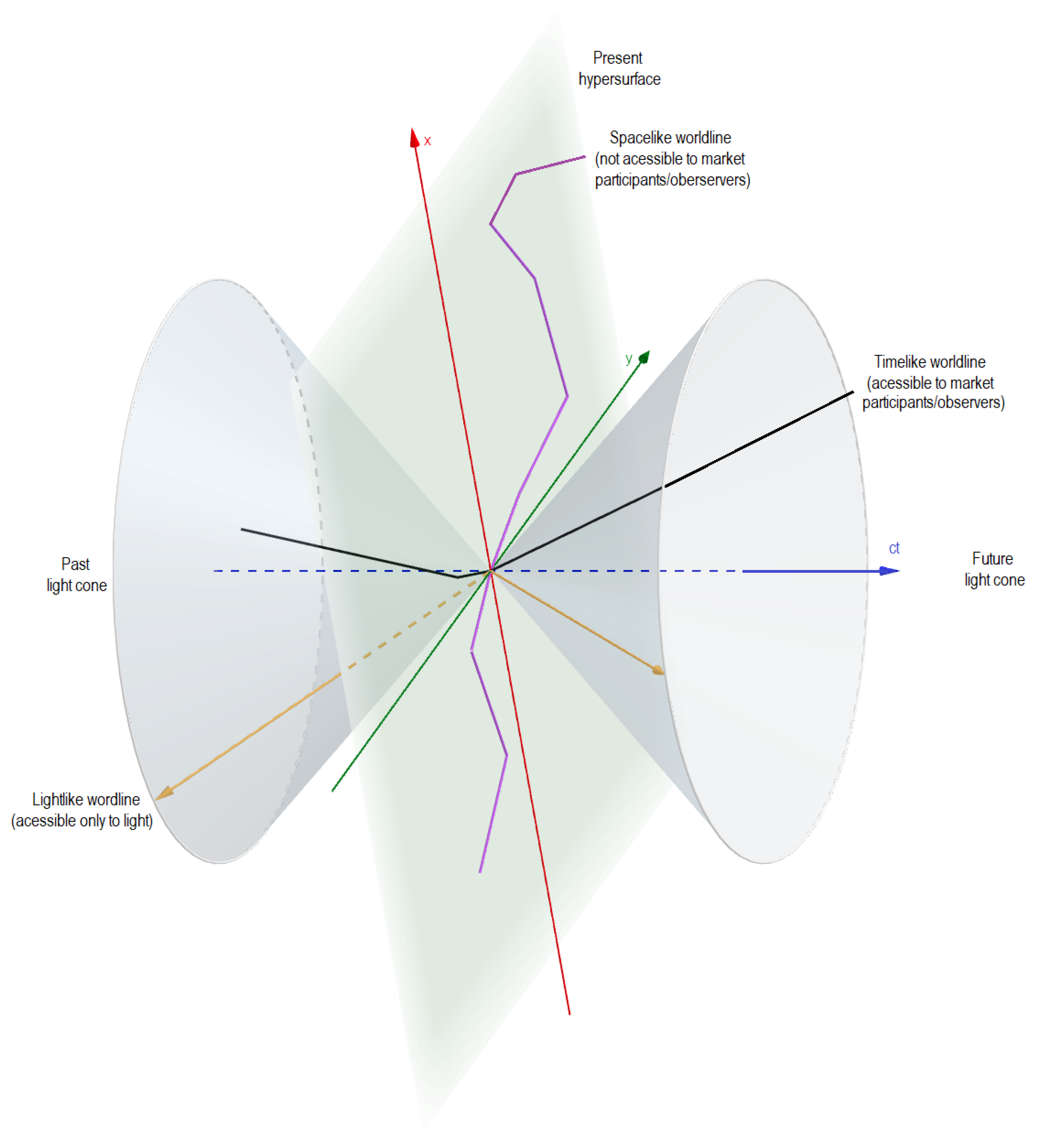
In relativity, representations like that of Figure 1 are widely used; however, with the equivalent time represented vertically. Here, we opted to represent it in the horizontal axis, which is typically the time-related axis in finance. We hope the change of axis will not be considered a physical “heresy” and that it will help those from a financial background to better visualize the concepts. It presents a spacetime diagram where the z axis is omitted. As events can take any direction and dimensions are isotropic, this produces a four-dimension cone called the light cone.5
There are two possible light cones for each event E at each moment in time, a past light cone and a future one. The light cone surface is only accessible to light, because the slope line is , between and x. Thus, the distance that light travels, in a vacuum, in one second6 is m, which is the same distance travelled in all axes. This means that a w displacement in the axis is the same w displacement value in the space axes. Inside the light cone resides the four-dimensional coordinates available to all real events defined at the origin. Events inside the cone are time-like events and correspond to all sets of coordinates available to the E or MP defined at the origin. Space-like events are not accessible to the MP because this implies speeds higher than c.
3.3. Lorentz Transformations
Suppose L and define, respectively, the stationary and moving inertial reference frames.7 Let us consider a market participant, MP, on the four dimension’s inertial reference frame L with the coordinates . Recall, all coordinates are in meters m, and time t is obtained by dividing by c. In addition, we have a second market participant, MP, on the four dimensions inertial reference frame with the coordinates . Furthermore, the reference frame is moving away from L, according to MP, with the velocity v. For an event E its coordinates transformation between the inertial reference frames L and , is provided by the Lorentz transformations
where is the so-called Lorentz factor (Rindler 1982).
Lorentz transformations show that time and space are not invariant but reference-frame dependent (Siklos 2011). In Equation (1), the transformed and axes coincide with the y and z axes, which, although standard, is a simplification and assumes the direction of motion happens only in the axis (Naber 2012)8.
3.3.1. Space Contraction and Time Dilation
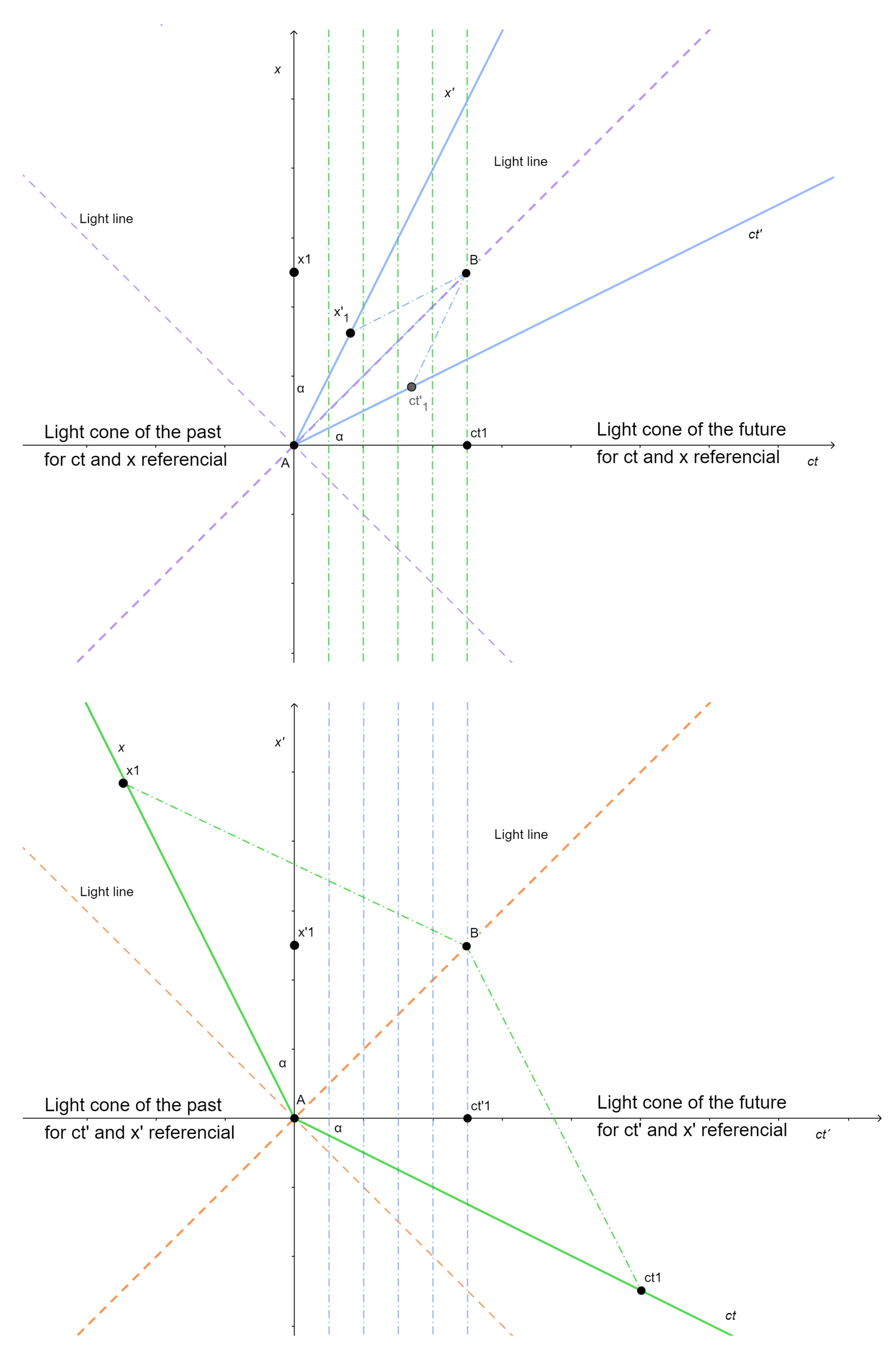
In Figure 2, the reference frames L and are drawn, only with , , x and axes, for the purposes of illustration. Green and light blue dashed lines represent simultaneity lines in the L and reference frames, respectively. The ratio between the reference frame’s relative velocity v and c, can also be defined as the arctan of the .9 The simultaneity line of is constant in the L; however, the simultaneity line of , represented on L, has a slope. Vice versa, i.e., the simultaneity line , in its own reference frame , has no slope. Space contraction and time dilation are implicit from the first two expressions in (1).
Let us consider the reference frame , where an event , starts at , finishes at and is stationary; thereby, . The time interval of is, therefore, . According to the L reference frame, however, the event start and finishing moments have the coordinates and . Since the reference frame is moving at a constant velocity v according to L, the time interval in L is . In conclusion, the time interval is shorter than in L; therefore, the time passage on is slower than on L, and thus from perspective, time dilates.
On the contrary, in terms of space, we find a contraction. Consider now a second event also taking place in but that is instantaneous, i.e., and has length . According to L, the event is, also measured instantaneously with its start and finishing coordinates and , respectively; thus, . Since the reference frame is moving at a constant velocity v, according to L, we have and . Since we have , the length in is expanded, or the space in L is contracted.
Overall, in , one experiences time dilation (time passes slowly) and a space contraction, relative to what happens in L. Suppose, for instance, that a market participant MP is in L and that another, MP, is in . MP at instant , perceives MP at , that is a moment in the past of . On the other hand, MP perceives MP at instant , already, i.e., at a moment that is in the future of .
Thus, an asset can be valued by MP with price at time , but since is not in the simultaneity line of , MP values it differently obtaining , different from . Both MP and MP may be correctly pricing the asset, from the point of view of their own reference frames, which are L and , respectively. The obtained difference in the asset price is explained by the time dilation and space contraction that MP really feels in the reference frame, relative to L. The price is a past value of the asset in L.
If we wish for MPs in different reference frames to trade with one another, they must agree on “fair” asset valuations. One way to achieve this is to use what is known as proper time, instead of coordinate time.
3.3.2. Proper Time
Minkowski (1908) introduced the concepts of proper time that is Lorentz invariant, i.e., it is the same to all , independently of their coordinate systems (Siklos 2011). In fact, proper time can be interpreted as the temporal length (distance10 between the event start and finishing moments), of a vector , which measures the passage of time—e.g., the lifetime or duration—of an event E, experienced by a MP.
Proper time, in L and , respectively, is defined as
where the subscripts i and f stand for the initial and final moments of an event.
The invariant result of Lemma 1 follows from Equation (1). This is also visible in Figure 2 where the distance between points A and B is the same on both L and .
Lemma 1.
Given two different reference frames, L and , with associated Lorentz transformations as in Equation (1), have equal proper times. That is, for and , we have
Proof.
If the vector joining events and is timelike, then . These are the events accessible to us. If , the vector is lightlike—only accessible to light speed—and when (implies complex numbers), the vector is spacelike—not accessible to us nor to light.
3.3.3. Example
Let us consider two market participants: MP and MP and a concrete possible trade11.
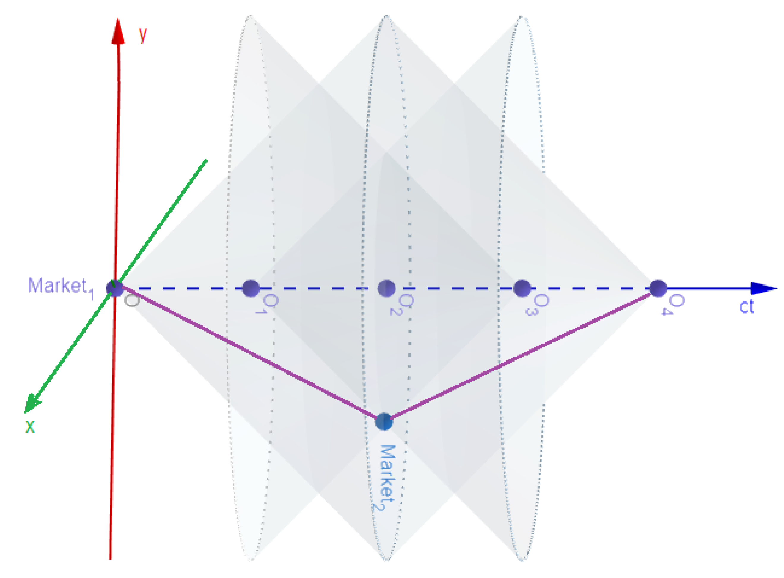
Figure 3 illustrates the situation, from the MP and MP perspectives. Past and future light cones for all relevant points are drawn. In this example, MP is stationary in a referential frame, and the time elapsed between points O and is T. The time interval between each consecutive point is .
Trade and MPs movements:
- At point in Market, (point O), MP and MP, agree on the price of an asset12.
- Then MP initiates a journey to Market.
- Exactly the moment when MP reaches Market is a simultaneous moment for MP. MP is at point and measures an elapsed time of T.
- Although from MP perspective, MP is at point . Thus, the elapsed time measured by MP is .
- From the Market perspective, the elapsed time is . Thus, when MP reaches Market, he sees the asset price for time (point ).
- According to MP, when MP reaches Market, he sees the asset price for T (point ).
- Now, let us consider if MP turns around and goes back to Market. While performing the turn, MP is not in an inertial reference frame, because MP has to slow down, turn and accelerate again.
- In this case, from MP’s perspective, while MP is turning back, the reality of MP shifts rapidly (from point to ).
- Although both meet back at point , in Market, MP spent time units, while for MP, it took longer—.
- Both MP and MP agree again on the asset price when they meet again at point (the law of one price holds)13. However one of them has experienced the possible gains or losses in less time than the other, which may be understood as some sort of “spacetime arbitrage”.
From the above description, it follows that, in the case where MPs—i.e., the buy and sell sides of a deal or regulation entities—are in different inertial reference frames, one needs to consider the spacetime structure, considering the associated Lorentz transformations and proper time.
The following axioms14 should hold.
- Axiom 1: For all financial events and market participants, when different inertial reference frames are involved, a settlement spacetime reference frame must be considered to serve as a benchmark.
- Axiom 2: When only time incorporates the relativity effects then proper time is the time measure that makes the asset or financial instrument pricing model invariant to all inertial reference frames. All market participants should follow the financial event proper time—i.e., deal or asset duration—to evaluate the asset or financial instrument pricing conditions.
4. Options
From the previous section, it follows that proper time is the right concept to measure an event’s lifetime and that this quantity is invariant. Therefore, when dealing with outer space or relativistic trading, one needs to re-define every event E—i.e., financial products, commercial deals, etc.—so that all , independently of their inertial reference frame, agree even if they are in different reference frame simultaneity lines.
That is, a "proper spacetime stamp" may be required for future deals, whenever need to consider different inertial frames. Haug (2004) refers to the possibility that the asset trade should register its own proper time and that this may be solved by implementing a spacetime stamp on each deal so that, independently of the MP times, they will all agree and follow, according to the assets deals, the spacetime stamp values.
In this section, we take the case of plain vanilla at-the-money (ATM) European options to illustrate the relativistic effects presented in the previous section. Essentially, an European call/put option is a contract that confers the holder the right, but not the obligation, to purchase/buy a certain underlying asset (e.g., a stock) for a fixed price K on a fixed expiry date T, after which the option becomes worthless. We consider the Black and Scholes (1973) model setup, as this is one of the greatest econophysics contributions to finance, where the heat diffusion equation, widely used in physics, helped to solve the problem of finding the fair price to option contracts.
Here, we focus only ATM calls/puts, i.e., the case when at inception , the strike price K equals the underlying asset current price s. Without a loss of generality, we also take . For simplicity, we also assume a zero interest rate . The fact that we consider interest rates to be zero allows us to focus on time dilation effects alone (avoiding mixed time effects resulting from discounting). We consider, that all stationary stay at rest for the entire life of the option. The moving maintain a constant speed (>0) from the inception at the end of the life of the option. This is a conceptualization; in reality, one can consider an average velocity for the while the life of the option elapses. The choice of plain vanilla ATM European options, with the conditions defined previously, instead of other assets, concerns the fact that Equation (4) is dependent only on volatility and time. This provides a better example to access the time dilation effects.
4.1. Pricing
For and , the option price depends on two key parameters: (i) the time to maturity and (ii) its volatility as follows from Lemma 2.
Lemma 2.
Considering the Black and Scholes (1973) model on a reference frame L, with and , the price at time t of an at-the-money call (or put) with time to maturity T and an underlying volatility σ is given by,
where stands for the cumulative distribution function for the Gaussian distribution.
Proof.
It follows from setting and in the standard Black–Scholes formula, . Under that setting, we also have . The result for puts follows from put-call parity when setting and . □
Let us consider a trade between two MPs who agree on the contract/settlement reference frame, L. That is, MP sells to MP, ATM calls for a given maturity T, at the “fair” premium in L.
Suppose, however, that after the deal is done, MP stays stationary in L, but MP starts a journey, moving relative to MP. MP is in a different reference frame and is also stationary in is frame.
For every day that is accounted on L—i.e., the coordinate time—less time is measured by MP on . Recall Figure 2.
Thus, from MP perspective, the option premium paid is higher than the "fair" theoretical premium, if MP had accounted for the time to maturity MP truly experienced, .
Proposition 1.
Under the same assumption as in Lemma 2, but for the perspective of the reference frame (as defined in Section 3), the “illusion”15 price at time t of the at-the-money call (or put) is given by,
where stands for the cumulative distribution function for the Gaussian distribution and γ is the Lorentz factor as defined in (1).
Proof.
Since the settlement reference frame is L, the contracted time to maturity is in L. However in , as the Lorentz transformation from Equation (1) applies. The result follows from the Lemma 2 solution with the same assumptions and by changing by . As before, put-call-parity guarantees , for and . □
To understand how sizable option price differences are, we also define the option price ratio, , with and as defined in Equations (4) and (5), respectively. We start by analysing the option prices in L and and their ratio for varying maturities, assuming a constant volatility .
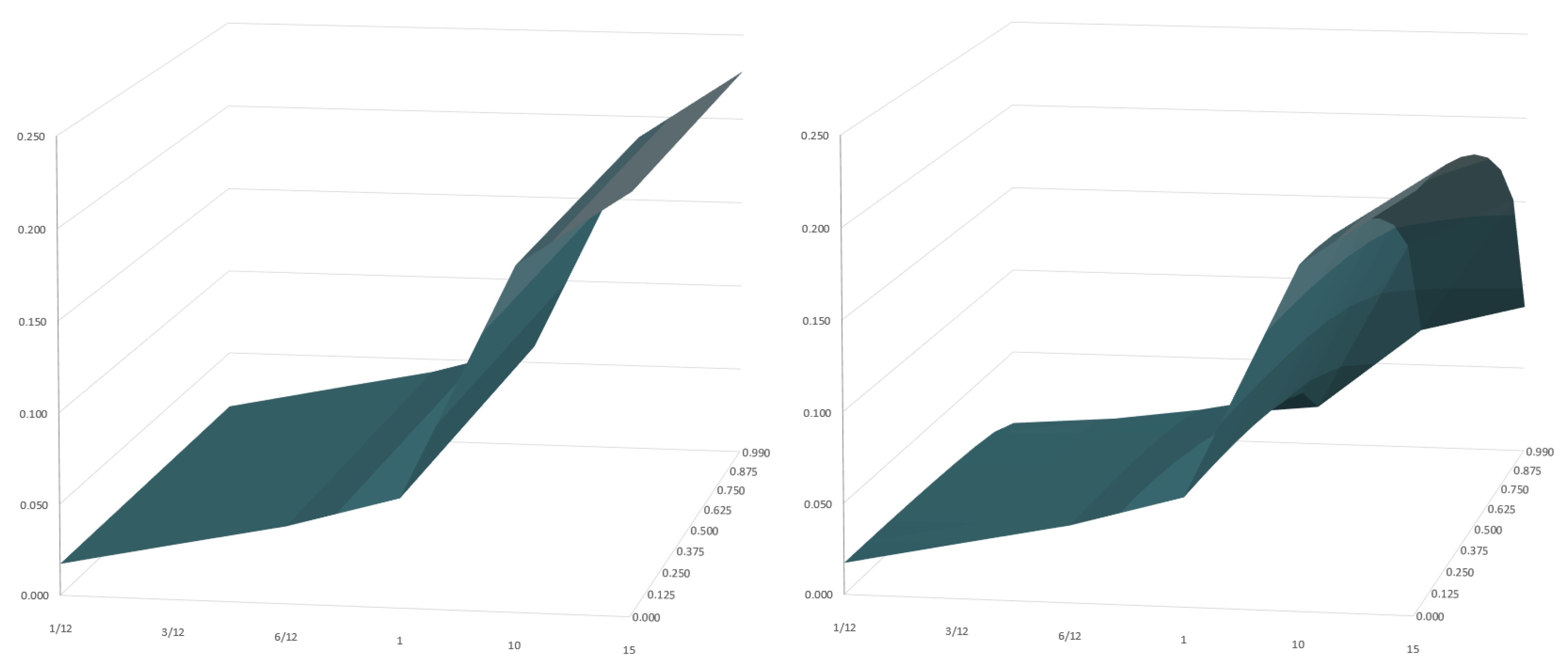
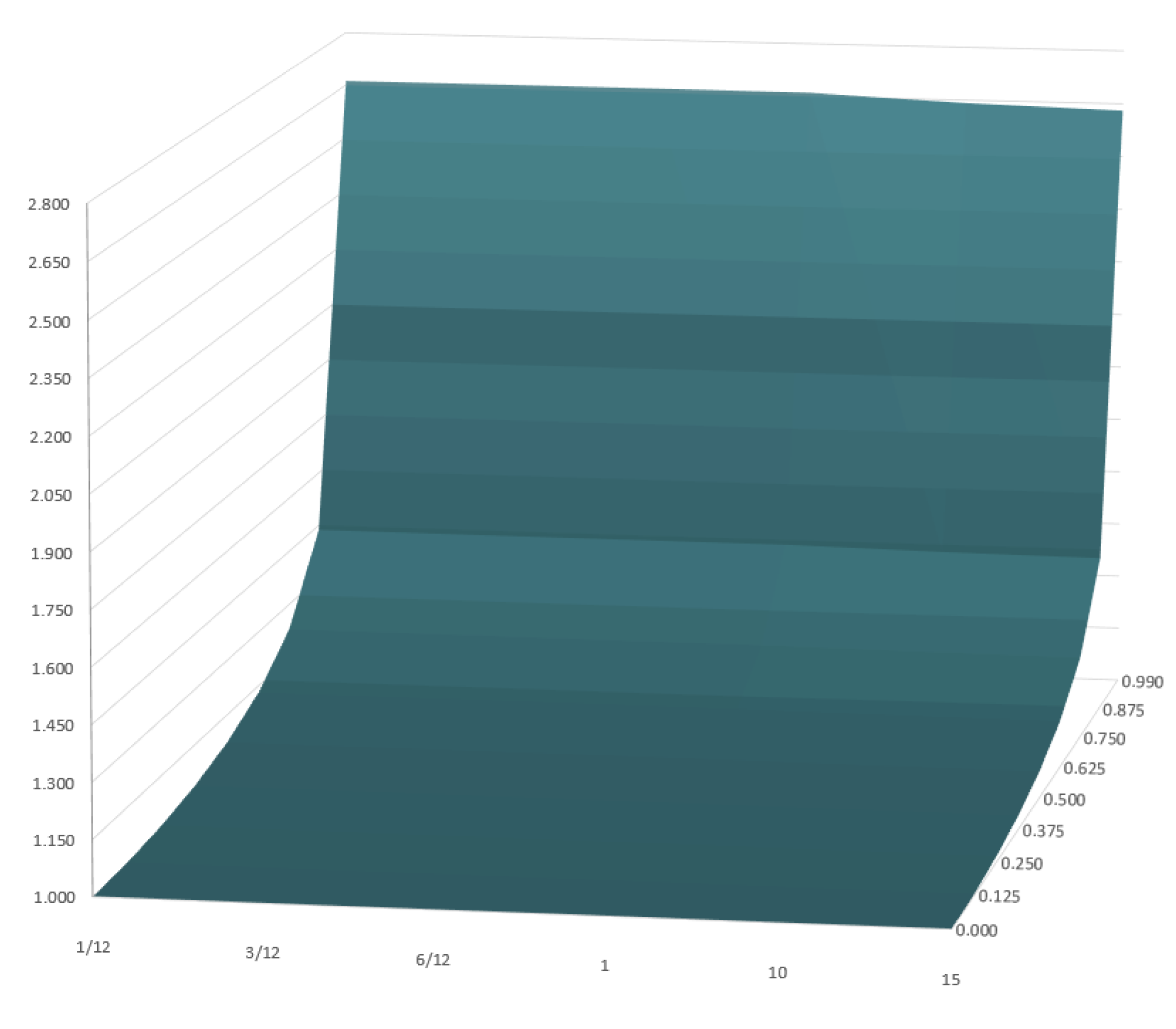
Figure 4 shows the option prices , surfaces for maturities T between 0 and 15 years and various velocities as a percentage of the light speed constant c. In Figure 5, a surface presents the ratio. Table 1 presents concrete values for the theoretical , prices and the ratio for the maturities and is divided in sets of different % of c velocity c = {0.0%, 12.5%, 25.0%, 37.5%, 50.0%, 62.5%, 75.0%, 87.5% and 99.0%}. As the velocity increases, so does the effect of relativity in the time dilation due to the factor. The prices increase relative to the settlement reference frame price . We considered maturities of 10 and 15 years to highlight the relativistic effects.
Both from the different shape in the price surfaces in L and , respectively, on the left and right of Figure 4 and from their ratio surface (Figure 5), it is clear that the differences in prices is non-negligible. The price surface in L is insensitive to velocity changes, as its is settlement reference frame. Naturally the prices of options increases with maturity. However, in terms of the reference frame, velocity does play an important role, as expected, in particular for high maturity options. It is clear that, as velocity increases, so does the time dilation and, correspondingly, the ratio between the two prices on the different referential frames. It is also important to notice that the price impact is considerable, as a ratio of 1.5 means is 50% higher than the .
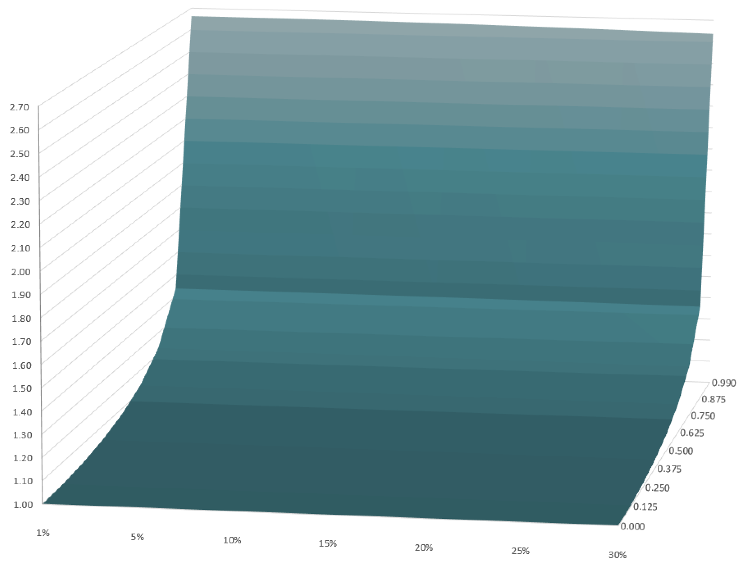
Figure 6 and Figure 7 show time dilation effects for volatility values ranging from 1% to 30%, for a fixed . Table 2 shows presents and prices and ratio for the volatility levels , for the % velocities of .
As expected, the time dilation effects become larger with increasing volatility. From Figure 6, it is clear from the right image that, for high volatility levels (above 15%), there starts to exist significant option price differences. These effects naturally depend on the velocity at which departs from L and become meaningful from 25% of the speed of light c. From the left image, we observe that, as expected, the option prices grow with volatility. The increase may seem almost linear in the image; however, it is not, as demonstrated by the values in Table 2. The almost non-visible non-linearity has to do with the relative short maturity chosen, .
The ratio in Figure 7 shows, as expected, higher price differences the higher the velocity under consideration is. Finally, although, for each fixed velocity, the ratios appear rather flat in volatility, that is not the case. This is better understood by looking at Table 2.
From the analysis in this section, it is clear that “relativistic arbitrages” are non negligible and that whenever relativistic effects take place, financial contracts should be redefined in a common time-like measure as for proper time.
Corollary 1.
Under the same assumption as in Lemma 2 and for both the settlement reference frame L and any other reference frame as defined in Section 3, the fair price at time t of an at-the-money call (or put) with time to maturity , on the settlement reference frame L and an underlying with volatility σ, is given by,
4.2. Some Greeks
We look now into the so-called greeks of options that measure the price sensitivity with respect to the various parameters. Given our assumptions concerning the moneyness () and interest rates (), the relevant statistics are the theta and vega.
4.2.1. Theta
The greek Theta gives us, in a ceteris paribus situation, the rate of change, as time passes, of the value, of an options portfolio.
Lemma 3.
From Lemma 2, for a reference frame L, with and , the time decay, or the rate of change of the value or an options portfolio, (Θ), of an at-the-money call (or put) with time to maturity T and an underlying with volatility σ is given by,
Proof.
This proceeds directly from the time partial derivative of Lemma 2. □
Lemma 4.
From Proposition 1, for a reference frame , with and , the time decay, or the rate of change of the value or an options portfolio, (), of an at-the-money call (or put) with time to maturity T and an underlying with volatility σ is given by,
Proof.
This proceeds directly from the time partial derivative of Proposition 1. □
Figure 8 shows the surface of the ratio /, for options with maturity year, for , , at inception , for the % velocities of and . is Theta for a reference frame that is moving and measures less time for velocities >0. For our special case, with , the values for and are equal to calls and puts. In Table 3, the values of , and /, per calendar day, can be verified.
The data show that the rate of change of the option value is lower for than for . This is due to the lesser time of the option life, measured by the moving , which is not in agreement with the time decay measured by the stationary . The moving , if travelling at a constant speed, measures less time than the one year of the option time to maturity. This accounts for the time decay for fewer days according to his reference frame.
4.2.2. Vega
The greek Vega presents us, in a ceteris paribus situation, the rate of change of the value of an options portfolio, with respect to the underlying asset volatility. is Vega for a reference frame that is moving and measures less time for velocities >0. For our special case, with , the values for and are equal to calls and puts. In Table 4, the values of , and /, per calendar day, can be verified.
Lemma 5.
From Lemma 2, for a reference frame L, with and , the rate of change of the value or an options portfolio, with respect to the underlying asset volatility, (ν), of an at-the-money call (or put) with time to maturity T and an underlying with volatility σ, is given by,
Proof.
This proceeds directly from the volatility partial derivative of Lemma 2. □
Lemma 6.
From Proposition 1, for a reference frame , with and , the rate of change of the value or an options portfolio, with respect to the underlying asset volatility, (), of an at-the-money call (or put) with time to maturity T and an underlying with volatility σ, is given by,
Proof.
This proceeds directly from the volatility partial derivative of Proposition 1. □
Lemma 7.
The ratio of / is equal to the ratio of /. From Lemmas 3–6 we have,
Proof.
This proceeds directly from Lemmas 3–6. □
Lemma 7 proves that, for a Call or a Put, the / and / ratios are equal. Consequently, Figure 8 presents both ratios. The data show that the rate of change of the option value, in respect to volatility is lower for than for . This is due to the lower time of the option’s life, measured by the moving , which is not in agreement with the time measured by the stationary . The moving , if travelling at a constant speed, measures less time than the one year of the option time to maturity; therefore, the volatility is reflected in a minor period. Lemma 2 and Proposition 1 prove, respectively, that and . A that is long in a portfolio of one (or a ), from reference frame L and long on a (or a ), from reference frame , measures the portfolio valuation given by . Table 5, presents the values for , and the difference for the volatilities 1.0%, 5.0%, 10.0%, 15.0%, 20.0%, 25.0% and 30.0%, for maturity year and for the velocities 0.0%, 12.5%, 25.0%, 37.5%, 50.0%, 62.5%, 75.0%, 87.5% and 99.0% of c. For simplicity, we consider the values at inception and and both asset prices at inception and strike equal to one .
5. Conclusions
This paper presents evidence for the future/theoretical need to incorporate relativity in finance models. Sooner or later, trading with market participants in different reference frames will be possible. At the same time, relativity has already begun to be introduced into financial models—sometimes without consistency. That is, more often than not, physical effects are used without taking into account their (physical) nature.
Here, we define key physical concepts and definitions and propose a simple market set up—based upon the special theory of relativity (STR)—to consider relativistic effects whenever market participants may belong to two (or more) different reference frames. To illustrate such effects in option pricing and hedging, we departed from the classical Black–Scholes model and showed that pricing and hedging ratios would vary considerably depending on which reference frame one considers. We showed that time dilation effects on the prices of plain vanilla European options were significant and particularly sizable for long maturity options on volatile underlings as the velocity grew. The sensitivity of prices—greeks—were also subject to meaningful effects.
Thus, to avoid arbitrages or erroneous evaluations, we propose the usage of the physical concept of proper time in the setup of financial contracts for market participants. In this manner, both prices and greeks would depend only on the proper time, which is invariant across different reference frames.
Overall, we established the following ”relativistic axioms”: (1) For all financial events and market participants, when different inertial reference frames are involved, a settlement spacetime reference frame must be considered to serve as a benchmark. (2) When only time incorporates relativity effects, then proper time is the time measure that makes the asset or financial instrument pricing model invariant, to all inertial reference frames. All market participants should follow the financial event proper time—i.e., deal or asset duration—to evaluate the asset or financial instrument pricing conditions.
The results here presented can be generalized to other assets. Natural candidates, due to the important effects time has on them, are fixed income instruments. The reason why we opted for options has to do with the fact that we could set the interest rate to be zero, while, when dealing with fixed income instruments, by definition, we cannot. By setting , we could focus on the time dilation effects alone, leaving the time value of money aside. The inclusion time value of money and its interaction with time dilation effects is the natural next step.
Taking a different direction, future studies can cover inertial reference frames with accelerations and gravity, moving toward the general theory of relativity (GTR) and bringing the theory developments to a more real scenario. Finally, developments may also be conducted regarding spatial arbitrage techniques, high frequency trading and by performing empirical test on models along with the introduction of relativity theory.
Author Contributions
Conceptualization, V.H.C.; methodology, V.H.C. and R.M.G.; software, V.H.C.; validation, R.M.G.; formal analysis, V.H.C. and R.M.G.; investigation, V.H.C.; resources, V.H.C. and R.M.G.; data curation, V.H.C.; writing—original draft preparation, V.H.C.; writing—review and editing, V.H.C. and R.M.G.; visualization, R.M.G.; supervision, R.M.G.; project administration, V.H.C. and R.M.G.; funding acquisition, VHC and R.M.G. All authors have read and agreed to the published version of the manuscript.
Funding
This research was was partially supported by the Project CEMAPRE/REM - UIDB/05069/2020 financed by FCT/MCTES through national funds.
Institutional Review Board Statement
Not applicable.
Informed Consent Statement
Not applicable.
Data Availability Statement
Resulted data is available from the authors upon request.
Conflicts of Interest
The authors declare no conflict of interest.
References
- Angel, James J. 2014. When finance meets physics: The impact of the speed of light on financial markets and their regulation. Financial Review 49: 271–81. [Google Scholar] [CrossRef] [Green Version]
- Auer, Markus P. 2015. Stranger Times: The Impact of Relativistic Time Concepts on the Time Value of Money. SSRN Electronic Journal, 1–16. [Google Scholar] [CrossRef]
- Bachelier, Louis. 1900. Théorie de la spéculation. Annales Scientifiques de l’École Normale Supérieure 17: 21–86. [Google Scholar] [CrossRef]
- Black, Fischer, and Myron Scholes. 1973. The Pricing of Options and Corporate Liabilities. The Journal of Political Economy 81: 637–54. [Google Scholar] [CrossRef] [Green Version]
- Buchanan, Mark. 2015. Physics in finance: Trading at the speed of light. Nature 518: 161–63. [Google Scholar] [CrossRef] [Green Version]
- Courtault, Jean-Michel, Youri Kabanov, Bernard Bru, Pierre Crépel, Isabelle Lebon, and Arnaud Le Marchand. 2000. Louis Bachelier on the Centenary of Théorie de la Spéculation. Mathematical Finance 10: 339–53. [Google Scholar] [CrossRef] [Green Version]
- de Area Leão Pereira, Eder Johnson, Marcus Fernandes da Silva, and H.B.B. Pereira. 2017. Econophysics: Past and present. Physica A: Statistical Mechanics and Its Applications 473: 251–61. [Google Scholar] [CrossRef]
- de Paula, João Antonio. 2002. Walras no Journal des Économistes: 1860–65. Revista Brasileira de Economia 56: 121–46. [Google Scholar] [CrossRef]
- Dunkel, Jörn, and Peter Hänggi. 2009. Relativistic Brownian motion. Physics Reports 471: 1–73. [Google Scholar] [CrossRef] [Green Version]
- Einstein, Albert. 1905. On the motion of small particles suspended in liquids at rest required by the molecular-kinetic theory of heat. Annalen der Physik 17: 208. [Google Scholar]
- Einstein, Albert. 1905. Zur Elektrodynamik bewegter Körper. Annalen der Physik 322: 891–921. [Google Scholar] [CrossRef]
- Einstein, Albert. 1916. Die Grundlage der allgemeinen Relativitätstheorie. Annalen der Physik 354: 769–822. [Google Scholar] [CrossRef] [Green Version]
- Eugene, Fama. 1970. Efficient Capital Market: A Re-view of Theory and Empirical Work. The Journal of Finance 25: 383–417. [Google Scholar]
- Fama, Eugene. 1991. Efficient capital markets II. The Journal of Finance XLVI: 1575–617. [Google Scholar] [CrossRef]
- Ferreira, Paulo, Éder J. A. L. Pereira, and Hernane B. B. Pereira. 2020. From Big Data to Econophysics and Its Use to Explain Complex Phenomena. Journal of Risk and Financial Management 13: 153. [Google Scholar] [CrossRef]
- Haug, Espen Gaarder. 2004. Space-time Finance. The relativity theory’s implications for mathematical finance. Willmott, July 2–15. [Google Scholar]
- Haug, Espen Gaarder. 2018. Double Light Speed: History, Confusion, and Recent Applications to High Speed Trading. SSRN Electronic Journal, 1–13. [Google Scholar] [CrossRef]
- Heisenberg, Werner. 1927. Über den anschaulichen Inhalt der quantentheoretischen Kinematik und Mechanik. Zeitschrift für Physik 43: 172–98. [Google Scholar] [CrossRef]
- Hetherington, Norriss S. 1983. Isaac Newton’s Influence on Adam Smith’s Natural Laws in Economics. Journal of the History of Ideas 44: 497–505. [Google Scholar] [CrossRef]
- Jacobson, Theodore, and Lawrence S. Schulman. 1984. Quantum stochastics: The passage from a relativistic to a non-relativistic path integral. Journal of Physics A: Mathematical and General 17: 375–83. [Google Scholar] [CrossRef] [Green Version]
- Kakushadze, Zura. 2017. Volatility smile as relativistic effect. Physica A: Statistical Mechanics and Its Applications 475: 59–76. [Google Scholar] [CrossRef] [Green Version]
- Krugman, Paul. 2010. The theory of interstellar trade. Economic Inquiry 48: 1119–23. [Google Scholar] [CrossRef]
- Laughlin, Gregory, Anthony Aguirre, and Joseph Grundfest. 2014. Information Transmission between Financial Markets in Chicago and New York. Financial Review 49: 283–312. [Google Scholar] [CrossRef]
- Mannix, Brian. 2016. Space-Time Trading: Special Relativity and Financial Market Microstructure. Columbian College of Arts & Sciences. [Google Scholar]
- Mantegna, Rosario N., and H.Eugene Stanley. 1999. Introduction to Econophysics: Correlations and Complexity in Finance. New York: Cambridge University Press, p. 148. [Google Scholar]
- Merton, Robert C. 1973. Theory of rational option pricing. The Bell Journal of Economics and Management Science 4: 141–83. [Google Scholar] [CrossRef] [Green Version]
- Minkowski, Hermann. 1908. Die Grundgleichungen für die elektromagnetischen Vorgänge in bewegten Körpern. Nachrichten von der Gesellschaft der Wissenschaften zu Göttingen, Mathematisch-Physikalische Klasse, 53–111. [Google Scholar]
- Mohajan, Haradhan. 2013. Minkowski geometry and space-time manifold in relativity. Journal of Environmental Treatment Techniques 1: 101–9. [Google Scholar]
- Morton, Jason. 2016. Relativistic Finance. Available online: Medium.com (accessed on 14 June 2021).
- Naber, Gregory L. 2012. The Geometry of Minkowski Spacetime. In Applied Mathematical Sciences. New York: Springer, vol. 92. [Google Scholar] [CrossRef]
- NASA. 2018. Mars Fact Sheet; Washington, DC: NASA.
- Pincak, Richard, and Kabin Kanjamapornkul. 2018. GARCH(1,1) Model of the Financial Market with the Minkowski Metric. Zeitschrift für Naturforschung A 73: 669–84. [Google Scholar] [CrossRef] [Green Version]
- Rindler, Wolfgang. 1982. Introduction to Special Relativity. Oxford: Oxford University Press. [Google Scholar]
- Romero, Juan M., and Ilse B. Zubieta-Martínez. 2016. Relativistic Quantum Finance. arXiv arXiv:1604.01447. [Google Scholar]
- Romero, Juan M., Ulises Lavana, and Elio Martínez. 2013. Schrödinger group and quantum finance. arXiv arXiv:1304.4995. [Google Scholar]
- Samuelson, Paul A. 1965. Proof That Properly Anticipated Prices Fluctuate Randomly. Management Review 6: 41–49. [Google Scholar]
- Saptsin, Vladimir, and Vladimir Soloviev. 2009. Relativistic quantum econophysics—New paradigms in complex systems modelling. arXiv arXiv:0907.1142. [Google Scholar]
- Savoiu, Gheorghe, and Ion Iorga Siman. 2013. History and role of econophysics in scientific research. In Econophysics Background and Applications in Economics, Finance, and Sociophysics. Edited by Gheorghe Săvoiu. Oxford: Academic Press, Chapter 1. pp. 3–16. [Google Scholar]
- Schinkus, Christophe. 2010. Is Econophysics a new discipline. Physica A 389: 3814–21. [Google Scholar] [CrossRef]
- Siklos, Stephen. 2011. Special Relativity. Cambridge: University of Cambridge. [Google Scholar]
- Stanley, H. Eugene, Viktor Afanasyev, Luis A. Nunes Amaral, Serguei V. Buldyrev, Ary L. Goldberger, Steve Havlin, Harry Leschhorn, Philipp H. Maass, Rosario N. Mantegna, C.-K. Peng, and et al. 1996. Anomalous fluctuations in the dynamics of complex systems: From DNA and physiology to econophysics. Physica A: Statistical Mechanics and Its Applications 224: 302–21. [Google Scholar] [CrossRef]
- Tenreiro Machado, J. A. 2014. Relativistic time effects in financial dynamics. Nonlinear Dynamics 75: 735–44. [Google Scholar] [CrossRef] [Green Version]
- Trzetrzelewski, Maciej. 2017. Relativistic Black-Scholes model. Europhysics Letters 117: 1–18. [Google Scholar] [CrossRef] [Green Version]
- Wissner-Gross, Alexander D., and Cameron E. Freer. 2010. Relativistic statistical arbitrage. Physical Review E-Statistical, Nonlinear, and Soft Matter Physics 82: 1–7. [Google Scholar] [CrossRef] [PubMed]
- Zumbach, Gilles O. 2007. Time Reversal Invariance in Finance. SSRN Electronic Journal. [Google Scholar] [CrossRef] [Green Version]
| 1 | The notion of spacetime is explained in Section 3. |
| 2 | The distance between the planets is not always the same. Planets have elliptical orbits around the Sun. All planets have different elliptics; therefore, the distance between them is not constant. |
| 3 | The term “event” also has a wider meaning—it can define a happening or an object. |
| 4 | It allows to create a metric tensor to perform coordinate transformations between different inertial reference frames. |
| 5 | Only three-dimensions are represented in Figure 1. |
| 6 | Recall m/s in a vacuum. |
| 7 | |
| 8 | The extension of this setup to other spacetime formulations is possible. For the purpose of this paper, the simplest Minkowski spacetime definition suffices. |
| 9 | |
| 10 | That is why, in some of the literature, proper time is also referred to as proper distance or a Minkowski interval. |
| 11 | This example can be understood as an adaptation, to a financial setting, of the well-known “Twin Paradox” (Siklos 2011). |
| 12 | Or other characteristic of the asset. For illustration purpose, we consider the price. |
| 13 | For this to happen MP and MP must have different pricing models for the asset price, as they experienced different time spans between their meetings. For instance, travelling in space for MP may be modelled using price jumps to account to for the time dilation experience, particularly when MP turns back and sees MP passing from to . |
| 14 | |
| 15 | Assuming only time dilation effects and not proper time. |
Figure 1.
A spacetime diagram with past and future light cones and timelike, lightlike and spacelike trajectory representation.
Figure 1.
A spacetime diagram with past and future light cones and timelike, lightlike and spacelike trajectory representation.

Figure 2.
L (top image) and (bottom image) spacetime representations.

Figure 3.
The two market participant case in a spacetime diagram.

Figure 4.
Surfaces of European ATM call (or put) prices (z-axis) in the reference frames L (left figure) and (right figure), for velocities ranging from to (y-axis) and maturities T (x-axis) of 1/12, 3/12, 6/12, 1, 10 and 15 years. The asset volatility is fixed at . For simplicity, we consider the values at inception and and both prices at inception and strike equal to one .

Figure 5.
Surface of the ratio / (or /), displayed on the z axis, for velocities ranging from to (y-axis) and maturities T (x-axis) of 1/12, 3/12, 6/12, 1, 10 and 15 years. The asset volatility is fixed at . For simplicity, we consider the values at inception and and both asset prices at inception and strike equal to one .

Figure 6.
Surfaces of European ATM call (or put) prices (z-axis) in the reference frames L (left figure) and (right figure), for velocities ranging from to (y-axis) and the volatilities (x-axis) of 1%, 5%, 10%, 15%, 20%, 25% and 30%, for maturity year. For simplicity, we consider values at inception , and both asset prices at inception and strike equal to one .

Figure 7.
Surface of the ratio / (or /), displayed on the z axis, for velocities ranging from to (y-axis) and volatilities (x-axis) of 1%, 5%, 10%, 15%, 20%, 25% and 30%, for maturity year. For simplicity, we consider the values at inception and and both asset prices at inception and strike equal to one .

Figure 8.
Surface of the ratio / (for a Call or Put), displayed on the z axis, for velocities ranging from to (y-axis) and the volatilities (x-axis) of 1%, 5%, 10%, 15%, 20%, 25% and 30%, for maturity year. For simplicity, we consider the values at inception and and both asset prices at inception and strike equal to one . is Theta for a reference frame that is moving and measures less time for velocities >0. Lemma 7’s proof shows that, for a Call or a Put, the / and / ratios are equal. Thus, Figure 8 presents both ratios. is Vega for a reference frame that is moving and measures less time for velocities >0.


Table 1.
Prices of , as well as the ratio, for the maturities 1/12, 3/12, 6/12, 1, 10 and 15 years and for the velocities 0.0%, 12.5%, 25.0%, 37.5%, 50.0%, 62.5%, 75.0%, 87.5% and 99.0% of c. The asset volatility is fixed at . For simplicity, we consider values at inception and and both asset prices at inception and strike equal to one .
| Velocity 0.0% of c | Velocity 12.5% of c | Velocity 25.0% of c | |||||||||
|---|---|---|---|---|---|---|---|---|---|---|---|
| T | Call | Call’ | Call/Call’ | T | Call | Call’ | Call/Call’ | T | Call | Call’ | Call/Call’ |
| 1/12 | 1.73% | 1.73% | 1.00000 | 1/12 | 1.73% | 1.72% | 1.00394 | 1/12 | 1.73% | 1.70% | 1.01626 |
| 3/12 | 2.99% | 2.99% | 1.00000 | 3/12 | 2.99% | 2.98% | 1.00394 | 3/12 | 2.99% | 2.94% | 1.01626 |
| 6/12 | 4.23% | 4.23% | 1.00000 | 6/12 | 4.23% | 4.21% | 1.00394 | 6/12 | 4.23% | 4.16% | 1.01625 |
| 1 | 5.98% | 5.98% | 1.00000 | 1 | 5.98% | 5.96% | 1.00394 | 1 | 5.98% | 5.88% | 1.01624 |
| 10 | 18.75% | 18.75% | 1.00000 | 10 | 18.75% | 18.68% | 1.00387 | 10 | 18.75% | 18.45% | 1.01597 |
| 15 | 22.85% | 22.85% | 1.00000 | 15 | 22.85% | 22.77% | 1.00384 | 15 | 22.85% | 22.50% | 1.01582 |
| Velocity 37.5% of c | Velocity 50.0% of c | Velocity 62.5% of c | |||||||||
| T | Call | Call’ | Call/Call | T | Call | Call’ | Call/Call’ | T | Call | Call’ | Call/Call’ |
| 1/12 | 1.73% | 1.66% | 1.03861 | 1/12 | 1.73% | 1.61% | 1.07456 | 1/12 | 1.73% | 1.53% | 1.13180 |
| 3/12 | 2.99% | 2.88% | 1.03860 | 3/12 | 2.99% | 2.78% | 1.07454 | 3/12 | 2.99% | 2.64% | 1.13177 |
| 6/12 | 4.23% | 4.07% | 1.03858 | 6/12 | 4.23% | 3.94% | 1.07450 | 6/12 | 4.23% | 3.74% | 1.13171 |
| 1 | 5.98% | 5.76% | 1.03854 | 1 | 5.98% | 5.56% | 1.07444 | 1 | 5.98% | 5.28% | 1.13159 |
| 10 | 18.75% | 18.06% | 1.03791 | 10 | 18.75% | 17.47% | 1.07323 | 10 | 18.75% | 16.60% | 1.12951 |
| 15 | 22.85% | 22.03% | 1.03756 | 15 | 22.85% | 21.31% | 1.07257 | 15 | 22.85% | 20.25% | 1.12837 |
| Velocity 75.0% of c | Velocity 87.5% of c | Velocity 99.0% of c | |||||||||
| T | Call | Call’ | Call/Call’ | T | Call | Call’ | Call/Call’ | T | Call | Call’ | Call/Call’ |
| 1/12 | 1.73% | 1.40% | 1.22954 | 1/12 | 1.73% | 1.20% | 1.43716 | 1/12 | 1.73% | 0.65% | 2.66230 |
| 3/12 | 2.99% | 2.43% | 1.22948 | 3/12 | 2.99% | 2.08% | 1.43704 | 3/12 | 2.99% | 1.12% | 2.66195 |
| 6/12 | 4.23% | 3.44% | 1.22938 | 6/12 | 4.23% | 2.94% | 1.43687 | 6/12 | 4.23% | 1.59% | 2.66141 |
| 1 | 5.98% | 4.86% | 1.22919 | 1 | 5.98% | 4.16% | 1.43652 | 1 | 5.98% | 2.25% | 2.66034 |
| 10 | 18.75% | 15.30% | 1.22570 | 10 | 18.75% | 13.11% | 1.43032 | 10 | 18.75% | 7.10% | 2.64122 |
| 15 | 22.85% | 18.68% | 1.22379 | 15 | 22.85% | 16.02% | 1.42691 | 15 | 22.85% | 8.69% | 2.63072 |
Table 2.
Prices for , as well as the ratio, for the volatilities 1.0%, 5.0%, 10.0%, 15.0%, 20.0%, 25.0% and 30.0%, for maturity year, for the velocities 0.0%, 12.5%, 25.0%, 37.5%, 50.0%, 62.5%, 75.0%, 87.5% and 99.0% of c. For simplicity, we consider the values at inception and and both asset priced at inception and strike equal to one .
| Velocity 0.0% of c | Velocity 12.5% of c | Velocity 25.0% of c | |||||||||
|---|---|---|---|---|---|---|---|---|---|---|---|
| Call | Call’ | Call/Call’ | Call | Call’ | Call/Call’ | Call | Call’ | Call/Call’ | |||
| 1% | 0.40% | 0.40% | 1.0000 | 1% | 0.40% | 0.40% | 1.0039 | 1% | 0.40% | 0.39% | 1.0163 |
| 5% | 1.99% | 1.99% | 1.0000 | 5% | 1.99% | 1.99% | 1.0039 | 5% | 1.99% | 1.96% | 1.0163 |
| 10% | 3.99% | 3.99% | 1.0000 | 10% | 3.99% | 3.97% | 1.0039 | 10% | 3.99% | 3.92% | 1.0163 |
| 15% | 5.98% | 5.98% | 1.0000 | 15% | 5.98% | 5.96% | 1.0039 | 15% | 5.98% | 5.88% | 1.0162 |
| 20% | 7.97% | 7.97% | 1.0000 | 20% | 7.97% | 7.93% | 1.0039 | 20% | 7.97% | 7.84% | 1.0162 |
| 25% | 9.95% | 9.95% | 1.0000 | 25% | 9.95% | 9.91% | 1.0039 | 25% | 9.95% | 9.79% | 1.0162 |
| 30% | 11.92% | 11.92% | 1.0000 | 30% | 11.92% | 11.88% | 1.0039 | 30% | 11.92% | 11.73% | 1.0161 |
| Velocity 37.5% of c | Velocity 50.0% of c | Velocity 62.5% of c | |||||||||
| Call | Call’ | Call/Call’ | Call | Call’ | Call/Call’ | Call | Call’ | Call/Call’ | |||
| 1% | 0.40% | 0.38% | 1.0386 | 1% | 0.40% | 0.37% | 1.0476 | 1% | 0.40% | 0.35% | 1.1318 |
| 5% | 1.99% | 1.92% | 1.0386 | 5% | 1.99% | 1.86% | 1.0746 | 5% | 1.99% | 1.76% | 1.1318 |
| 10% | 3.99% | 3.84% | 1.0386 | 10% | 3.99% | 3.71% | 1.0745 | 10% | 3.99% | 3.52% | 1.1317 |
| 15% | 5.98% | 5.76% | 1.0385 | 15% | 5.98% | 5.56% | 1.0744 | 15% | 5.98% | 5.28% | 1.1316 |
| 20% | 7.97% | 7.67% | 1.0385 | 20% | 7.97% | 7.41% | 1.0743 | 20% | 7.97% | 7.04% | 1.1314 |
| 25% | 9.95% | 9.58% | 1.0384 | 25% | 9.95% | 9.26% | 1.0742 | 25% | 9.95% | 8.79% | 1.1312 |
| 30% | 11.92% | 11.48% | 1.0383 | 30% | 11.92% | 11.10% | 1.0740 | 30% | 11.92% | 10.54% | 1.1309 |
| Velocity 75.0% of c | Velocity 87.5% of c | Velocity 99.0% of c | |||||||||
| Call | Call’ | Call/Call’ | Call | Call’ | Call/Call’ | Call | Call’ | Call/Call’ | |||
| 1% | 0.40% | 0.28% | 1.2296 | 1% | 0.40% | 0.28% | 1.4372 | 1% | 0.40% | 0.15% | 2.6625 |
| 5% | 1.99% | 1.39% | 1.2295 | 5% | 1.99% | 1.39% | 1.4371 | 5% | 1.99% | 0.75% | 2.6622 |
| 10% | 3.99% | 2.78% | 1.2294 | 10% | 3.99% | 2.78% | 1.4369 | 10% | 3.99% | 1.50% | 2.6615 |
| 15% | 5.98% | 4.16% | 1.2292 | 15% | 5.98% | 4.16% | 1.4365 | 15% | 5.98% | 2.25% | 2.6603 |
| 20% | 7.97% | 5.55% | 1.2289 | 20% | 7.97% | 5.55% | 1.4360 | 20% | 7.97% | 3.00% | 2.6587 |
| 25% | 9.95% | 6.93% | 1.2285 | 25% | 9.95% | 6.93% | 1.4353 | 25% | 9.95% | 3.74% | 2.6565 |
| 30% | 11.92% | 8.31% | 1.2280 | 30% | 11.92% | 8.31% | 1.4344 | 30% | 11.92% | 4.49% | 2.6539 |
Table 3.
Values for , and the ratio / (for a Call or Put), per calendar day, for the volatilities 1.0%, 5.0%, 10.0%, 15.0%, 20.0%, 25.0% and 30.0%, for maturity year and for the velocities 0.0%, 12.5%, 25.0%, 37.5%, 50.0%, 62.5%, 75.0%, 87.5% and 99.0% of c. For simplicity, we consider the values at inception and and both asset prices at inception and strike equal to one . is Theta for a reference frame that is moving and measures less time for velocities >0.
| Velocity 0.0% of c | Velocity 12.5% of c | Velocity 25.0% of c | |||||||||
|---|---|---|---|---|---|---|---|---|---|---|---|
| Theta | Theta’ | Theta/Theta’ | Theta | Theta’ | Theta/Theta’ | Theta | Theta’ | Theta/Theta’ | |||
| 1% | −0.001995 | −0.001995 | 1.000000 | 1% | −0.001995 | −0.001987 | 1.003945 | 1% | −0.001995 | −0.001963 | 1.016265 |
| 5% | −0.009970 | −0.009970 | 1.000000 | 5% | −0.009970 | −0.009931 | 1.003942 | 5% | −0.009970 | −0.009811 | 1.016255 |
| 10% | −0.019922 | −0.019922 | 1.000000 | 10% | −0.019922 | −0.019844 | 1.003935 | 10% | −0.019922 | −0.019604 | 1.016225 |
| 15% | −0.029837 | −0.029837 | 1.000000 | 15% | −0.029837 | −0.029720 | 1.003923 | 15% | −0.029837 | −0.029362 | 1.016175 |
| 20% | −0.039695 | −0.039695 | 1.000000 | 20% | −0.039695 | −0.039541 | 1.003905 | 20% | −0.039695 | −0.039066 | 1.016104 |
| 25% | −0.049480 | −0.049480 | 1.000000 | 25% | −0.049480 | −0.049288 | 1.003883 | 25% | −0.049480 | −0.048700 | 1.016013 |
| 30% | −0.059172 | −0.059172 | 1.000000 | 30% | −0.059172 | −0.058945 | 1.003856 | 30% | −0.059172 | −0.058246 | 1.015903 |
| Velocity 37.5% of c | Velocity 50.0% of c | Velocity 62.5% of c | |||||||||
| Theta | Theta’ | Theta/Theta’ | Theta | Theta’ | Theta/Theta’ | Theta | Theta’ | Theta/Theta’ | |||
| 1% | −0.001995 | −0.001921 | 1.038613 | 1% | −0.001995 | −0.001856 | 1.074568 | 1% | −0.001995 | −0.001762 | 1.131821 |
| 5% | −0.009970 | −0.009600 | 1.038591 | 5% | −0.009970 | −0.009279 | 1.074525 | 5% | −0.009970 | −0.008810 | 1.131746 |
| 10% | −0.019922 | −0.019183 | 1.038520 | 10% | −0.019922 | −0.018543 | 1.074390 | 10% | −0.019922 | −0.017607 | 1.131514 |
| 15% | −0.029837 | −0.028733 | 1.038401 | 15% | −0.029837 | −0.027777 | 1.074165 | 15% | −0.029837 | −0.026378 | 1.131126 |
| 20% | −0.039695 | −0.038233 | 1.038235 | 20% | −0.039695 | −0.036965 | 1.073850 | 20% | −0.039695 | −0.035110 | 1.130583 |
| 25% | −0.049480 | −0.047667 | 1.038022 | 25% | −0.049480 | −0.046094 | 1.073446 | 25% | −0.049480 | −0.043792 | 1.129886 |
| 30% | −0.059172 | −0.057019 | 1.037762 | 30% | −0.059172 | −0.055149 | 1.072952 | 30% | −0.059172 | −0.052409 | 1.129034 |
| Velocity 75.0% of c | Velocity 87.5% of c | Velocity 99.0% of c | |||||||||
| Theta | Theta’ | Theta/Theta’ | Theta | Theta’ | Theta/Theta’ | Theta | Theta’ | Theta/Theta’ | |||
| 1% | −0.001995 | −0.001622 | 1.229571 | 1% | −0.001995 | −0.001388 | 1.437207 | 1% | −0.001995 | −0.000749 | 2.662454 |
| 5% | −0.009970 | −0.008110 | 1.229446 | 5% | −0.009970 | −0.006938 | 1.436985 | 5% | −0.009970 | −0.003746 | 2.661768 |
| 10% | −0.019922 | −0.016209 | 1.229056 | 10% | −0.019922 | −0.013871 | 1.436290 | 10% | −0.019922 | −0.007491 | 2.659625 |
| 15% | −0.029837 | −0.024289 | 1.228406 | 15% | −0.029837 | −0.020790 | 1.435133 | 15% | −0.029837 | −0.011233 | 2.656058 |
| 20% | −0.039695 | −0.032338 | 1.227497 | 20% | −0.039695 | −0.027691 | 1.433514 | 20% | −0.039695 | −0.014973 | 2.651072 |
| 25% | −0.049480 | −0.040348 | 1.226328 | 25% | −0.049480 | −0.034566 | 1.431436 | 25% | −0.049480 | −0.018709 | 2.644676 |
| 30% | −0.059172 | −0.048307 | 1.224902 | 30% | −0.059172 | −0.041411 | 1.428900 | 30% | −0.059172 | −0.022440 | 2.636879 |
Table 4.
Values for , and the ratio / (for a Call or Put), per calendar day, for the volatilities 1.0%, 5.0%, 10.0%, 15.0%, 20.0%, 25.0% and 30.0%, for maturity year and for the velocities 0.0%, 12.5%, 25.0%, 37.5%, 50.0%, 62.5%, 75.0%, 87.5% and 99.0% of c. For simplicity, we consider the values at inception and and both asset prices at inception and strike equal to one . is vega for a reference frame that is moving and measures less time for velocities >0.
| Velocity 0.0% of c | Velocity 12.5% of c | Velocity 25.0% of c | |||||||||
|---|---|---|---|---|---|---|---|---|---|---|---|
| Vega | Vega’ | Vega/Vega’ | Vega | Vega’ | Vega/Vega’ | Vega | Vega’ | Vega/Vega’ | |||
| 1% | 0.398937 | 0.398937 | 1.000000 | 1% | 0.398937 | 0.397370 | 1.003945 | 1% | 0.398937 | 0.392552 | 1.016265 |
| 5% | 0.398818 | 0.398818 | 1.000000 | 5% | 0.398818 | 0.397252 | 1.003942 | 5% | 0.398818 | 0.392438 | 1.016255 |
| 10% | 0.398444 | 0.398444 | 1.000000 | 10% | 0.398444 | 0.396882 | 1.003935 | 10% | 0.398444 | 0.392082 | 1.016225 |
| 15% | 0.397822 | 0.397822 | 1.000000 | 15% | 0.397822 | 0.396267 | 1.003923 | 15% | 0.397822 | 0.391490 | 1.016175 |
| 20% | 0.396953 | 0.396953 | 1.000000 | 20% | 0.396953 | 0.395408 | 1.003905 | 20% | 0.396953 | 0.390661 | 1.016104 |
| 25% | 0.395838 | 0.395838 | 1.000000 | 25% | 0.395838 | 0.394306 | 1.003883 | 25% | 0.395838 | 0.389599 | 1.016013 |
| 30% | 0.394479 | 0.394479 | 1.000000 | 30% | 0.394479 | 0.392964 | 1.003856 | 30% | 0.394479 | 0.388304 | 1.015903 |
| Velocity 37.5% of c | Velocity 50.0% of c | Velocity 62.5% of c | |||||||||
| Vega | Vega’ | Vega/Vega’ | Vega | Vega’ | Vega/Vega’ | Vega | Vega’ | Vega/Vega’ | |||
| 1% | 0.398937 | 0.384106 | 1.038613 | 1% | 0.398937 | 0.371254 | 1.074568 | 1% | 0.398937 | 0.324452 | 1.131821 |
| 5% | 0.398818 | 0.383999 | 1.038591 | 5% | 0.398818 | 0.371157 | 1.074525 | 5% | 0.398818 | 0.324388 | 1.131746 |
| 10% | 0.398444 | 0.383665 | 1.038520 | 10% | 0.398444 | 0.370856 | 1.074390 | 10% | 0.398444 | 0.324187 | 1.131514 |
| 15% | 0.397822 | 0.383110 | 1.038401 | 15% | 0.397822 | 0.370354 | 1.074165 | 15% | 0.397822 | 0.323852 | 1.131126 |
| 20% | 0.396953 | 0.382334 | 1.038235 | 20% | 0.396953 | 0.369654 | 1.073850 | 20% | 0.396953 | 0.323384 | 1.130583 |
| 25% | 0.395838 | 0.381338 | 1.038022 | 25% | 0.395838 | 0.368754 | 1.073446 | 25% | 0.395838 | 0.322783 | 1.129886 |
| 30% | 0.394479 | 0.380125 | 1.037762 | 30% | 0.394479 | 0.367658 | 1.072952 | 30% | 0.394479 | 0.322050 | 1.129034 |
| Velocity 75.0% of c | Velocity 87.5% of c | Velocity 99.0% of c | |||||||||
| Vega | Vega’ | Vega/Vega’ | Vega | Vega’ | Vega/Vega’ | Vega | Vega’ | Vega/Vega’ | |||
| 1% | 0.398937 | 0.324452 | 1.229571 | 1% | 0.398937 | 0.277578 | 1.437207 | 1% | 0.398937 | 0.149838 | 2.662454 |
| 5% | 0.398818 | 0.324388 | 1.229446 | 5% | 0.398818 | 0.277538 | 1.436985 | 5% | 0.398818 | 0.149832 | 2.661768 |
| 10% | 0.398444 | 0.324187 | 1.229056 | 10% | 0.398444 | 0.277412 | 1.436290 | 10% | 0.398444 | 0.149812 | 2.659625 |
| 15% | 0.397822 | 0.323852 | 1.228406 | 15% | 0.397822 | 0.277202 | 1.435133 | 15% | 0.397822 | 0.149779 | 2.656058 |
| 20% | 0.396953 | 0.323384 | 1.227497 | 20% | 0.396953 | 0.276909 | 1.433514 | 20% | 0.396953 | 0.149733 | 2.651072 |
| 25% | 0.395838 | 0.322783 | 1.226328 | 25% | 0.395838 | 0.276532 | 1.431436 | 25% | 0.395838 | 0.149673 | 2.644676 |
| 30% | 0.394479 | 0.322050 | 1.224902 | 30% | 0.394479 | 0.276072 | 1.428900 | 30% | 0.394479 | 0.149601 | 2.636879 |
Table 5.
Values for , and the difference for , volatilities 1.0%, 5.0%, 10.0%, 15.0%, 20.0%, 25.0% and 30.0%, and for velocities 0.0%, 12.5%, 25.0%, 37.5%, 50.0%, 62.5%, 75.0%, 87.5% and 99.0% of c. For simplicity, we consider the values at inception , and both asset prices at inception and strike equal to one . Lemma 2 and Proposition 1 prove, respectively, that and .
| Velocity 0.0% of c | Velocity 12.5% of c | Velocity 25.0% of c | |||||||||
|---|---|---|---|---|---|---|---|---|---|---|---|
| Call | Call’ | Call-Put’ = Put-Call’ | Call | Call’ | Call-Put’ = Put-Call’ | Call | Call’ | Call-Put’ = Put-Call’ | |||
| 1% | 0.40% | 0.40% | 0.000% | 1% | 0.40% | 0.40% | 0.002% | 1% | 0.40% | 0.39% | 0.006% |
| 5% | 1.99% | 1.99% | 0.000% | 5% | 1.99% | 1.99% | 0.008% | 5% | 1.99% | 1.96% | 0.032% |
| 10% | 3.99% | 3.99% | 0.000% | 10% | 3.99% | 3.97% | 0.016% | 10% | 3.99% | 3.92% | 0.064% |
| 15% | 5.98% | 5.98% | 0.000% | 15% | 5.98% | 5.96% | 0.023% | 15% | 5.98% | 5.88% | 0.096% |
| 20% | 7.97% | 7.97% | 0.000% | 20% | 7.97% | 7.93% | 0.031% | 20% | 7.97% | 7.84% | 0.127% |
| 25% | 9.95% | 9.95% | 0.000% | 25% | 9.95% | 9.91% | 0.039% | 25% | 9.95% | 9.79% | 0.158% |
| 30% | 11.92% | 11.92% | 0.000% | 30% | 11.92% | 11.88% | 0.047% | 30% | 11.92% | 11.73% | 0.189% |
| Velocity 37.5% of c | Velocity 50.0% of c | Velocity 62.5% of c | |||||||||
| Call | Call’ | Call-Put’ = Put-Call’ | Call | Call’ | Call-Put’ = Put-Call’ | Call | Call’ | Call-Put’ = Put-Call’ | |||
| 1% | 0.40% | 0.38% | 0.015% | 1% | 0.40% | 0.37% | 0.028% | 1% | 0.40% | 0.35% | 0.046% |
| 5% | 1.99% | 1.92% | 0.074% | 5% | 1.99% | 1.86% | 0.138% | 5% | 1.99% | 1.76% | 0.232% |
| 10% | 3.99% | 3.84% | 0.148% | 10% | 3.99% | 3.71% | 0.277% | 10% | 3.99% | 3.52% | 0.464% |
| 15% | 5.98% | 5.76% | 0.222% | 15% | 5.98% | 5.56% | 0.414% | 15% | 5.98% | 5.28% | 0.695% |
| 20% | 7.97% | 7.67% | 0.295% | 20% | 7.97% | 7.41% | 0.551% | 20% | 7.97% | 7.04% | 0.925% |
| 25% | 9.95% | 9.58% | 0.368% | 25% | 9.95% | 9.26% | 0.687% | 25% | 9.95% | 8.79% | 1.154% |
| 30% | 11.92% | 11.48% | 0.440% | 30% | 11.92% | 11.10% | 0.822% | 30% | 11.92% | 10.54% | 1.380% |
| Velocity 75.0% of c | Velocity 87.5% of c | Velocity 99.0% of c | |||||||||
| Call | Call’ | Call-Put’ = Put-Call’ | Call | Call’ | Call-Put’ = Put-Call’ | Call | Call’ | Call-Put’ = Put-Call’ | |||
| 1% | 0.40% | 0.28% | 0.121% | 1% | 0.40% | 0.28% | 0.121% | 1% | 0.40% | 0.15% | 0.249% |
| 5% | 1.99% | 1.39% | 0.607% | 5% | 1.99% | 1.39% | 0.607% | 5% | 1.99% | 0.75% | 1.245% |
| 10% | 3.99% | 2.78% | 1.213% | 10% | 3.99% | 2.78% | 1.213% | 10% | 3.99% | 1.50% | 2.489% |
| 15% | 5.98% | 4.16% | 1.817% | 15% | 5.98% | 4.16% | 1.817% | 15% | 5.98% | 2.25% | 3.731% |
| 20% | 7.97% | 5.55% | 2.418% | 20% | 7.97% | 5.55% | 2.418% | 20% | 7.97% | 3.00% | 4.970% |
| 25% | 9.95% | 6.93% | 3.017% | 25% | 9.95% | 6.93% | 3.017% | 25% | 9.95% | 3.74% | 6.203% |
| 30% | 11.92% | 8.31% | 3.611% | 30% | 11.92% | 8.31% | 3.611% | 30% | 11.92% | 4.49% | 7.431% |
Publisher’s Note: MDPI stays neutral with regard to jurisdictional claims in published maps and institutional affiliations. |
© 2021 by the authors. Licensee MDPI, Basel, Switzerland. This article is an open access article distributed under the terms and conditions of the Creative Commons Attribution (CC BY) license (https://creativecommons.org/licenses/by/4.0/).
Share and Cite
MDPI and ACS Style
Carvalho, V.H.; Gaspar, R.M. Relativistic Option Pricing. Int. J. Financial Stud. 2021, 9, 32. https://0-doi-org.brum.beds.ac.uk/10.3390/ijfs9020032
AMA Style
Carvalho VH, Gaspar RM. Relativistic Option Pricing. International Journal of Financial Studies. 2021; 9(2):32. https://0-doi-org.brum.beds.ac.uk/10.3390/ijfs9020032
Chicago/Turabian StyleCarvalho, Vitor H., and Raquel M. Gaspar. 2021. "Relativistic Option Pricing" International Journal of Financial Studies 9, no. 2: 32. https://0-doi-org.brum.beds.ac.uk/10.3390/ijfs9020032
Note that from the first issue of 2016, this journal uses article numbers instead of page numbers. See further details here.