
The Relation between Intraday Limit Order Book Depth and Spread


College of Business, University of Houston-Victoria, Victoria, TX 77901, USA
*
Author to whom correspondence should be addressed.
Int. J. Financial Stud. 2021, 9(4), 60; https://0-doi-org.brum.beds.ac.uk/10.3390/ijfs9040060
Submission received: 17 September 2021
/
Revised: 20 October 2021
/
Accepted: 22 October 2021
/
Published: 1 November 2021
Abstract
:Prior studies that examine the relation between market depth and bid–ask spread are often limited to the first level of the limit order book. However, the full limit order book provides important information beyond the first level about the depth and spread, which affects the trading decisions of market participants. This paper examines the intraday behavior of depth and spread in the five-deep limit order book and the relation between depth and spread in a futures market setting. A dummy-variables regression framework is employed and is estimated using the generalized method of moments (GMM). Results indicate an inverse U-shaped pattern for depth and an increasing pattern for spread. After controlling for known explanatory factors, an inverse relation between the limit order book depth and spread is documented. The inverse relation holds for depth and spread at individual levels in the limit order book as well. Results indicate that market participants actively manage both the price (spread) and quantity (depth) dimensions of liquidity along the five-deep limit order book.
1. Introduction
Finance literature shows that liquidity includes both a quantity dimension (depth) and a cost dimension (spread). Harris (1991) defines liquidity as the willingness of some traders to take the opposite side of a trade at a low cost. In other words, in a liquid market, many traders are willing to transact (provide a large depth) at a low cost (a small spread). Market participants can adjust to changing market conditions by modifying the quantity and/or the cost dimensions. For example, suppose there is an indication that the probability of informed trading in a market has increased. In that case, market participants can react by either adjusting the spread or the quantity available. In addition, Lee et al. (1993) argue that inferences about liquidity shifts cannot be made based on depth or spread alone but instead must be considered contemporaneously.
Although the interaction between depth and spread is a topic considered in prior research, the focus of most of these studies is the depth and spread at the best (first) level. For example, Vo (2007) employs the best depth and spread and finds an inverse intraday relation between the first level of depth and the first level of spread, meaning that traders actively manage both the price and quantity dimensions of liquidity at the best bid–ask level.
On the other hand, very little research focuses on the interaction between depth and spread beyond the first level, especially for futures markets. Depth beyond the best level illustrates how much trading interest exists at a particular price level. Similarly, limit order book depth illustrates the degree of order flow for the market at specific relative prices. Therefore, understanding the characteristics of depth in the limit order book is essential for both market makers and market participants. Prior research in other markets shows that the amount of depth in the limit order book provides important information concerning the trading decisions of market participants (Parlour 1998; Biais et al. 1995; Chiu et al. 2014; Aitken et al. 2007). In addition, Cao et al. (2009) find that the use of depth information past the best bid and ask also contributes to the price discovery process. Hautsch and Huang (2012) examine the market impact of limit orders on the state of the limit order book and show that aggressive limit orders have significant market impacts. Related research attempts to model the liquidity characteristics within the limit order book (Bouchaud et al. 2002; Yura et al. 2014). Aidov and Daigler (2015) examine the liquidity characteristics of the limit order book in futures markets but do not explore the relation between depth and spread.
In this paper, the relation between market depth and bid–ask spread is examined in aggregation and at individual levels in the limit order book. In addition, the intraday behavior of depth and spread is studied for the electronic futures market. The temporal variations of depth and spread and their interactions are examined in past research. However, most of these studies only employ depth at the best bid–ask spread level. The use of depth at only the best level is due to the lack of available data at deeper levels. Lee et al. (1993) examine the intraday shape of depth and spread for New York Stock Exchange (NYSE) stocks, finding a narrow depth at both the opening and closing of trading relative to the middle of the day, i.e., an inverted U-shaped pattern. Such a pattern is opposite to the pattern for the bid–ask spread, which possesses wide spreads at both the open and close of the trading day. However, Lee et al. (1993) do not employ control variables or test for the statistical significance of the depth and spread patterns.
Brockman and Chung (2000) investigate the temporal behavior of depth on the Stock Exchange of Hong Kong (SEHK), determining that an inverted U-shaped depth pattern exists. Although they employ control variables for known systematic factors that affect the depth, their measure of depth does not use depth beyond the first level. In addition, Vo (2007) examines the relation between depth and spread and their respective intraday patterns for Toronto Stock Exchange stocks. The study finds a U-shaped intraday bid–ask spread pattern and an intraday depth pattern that is increasing over the day with a narrow depth at the market open and a wide depth at the market close. Moreover, the presented relation between the depth and spread is negative.
The intraday behavior of depth and spread for three interest rate futures contracts on the Sydney Futures Exchange (SFE) is explored by Frino et al. (2008). An increasing intraday depth pattern, characterized by a small depth at the open and a large depth at the close, is documented at the best depth level. In addition, the spread pattern is opposite the depth pattern, with large spreads at the open and small spreads at the close. Their article models the relation between the depth and spread but does not consider depth beyond the first level.
In contrast, Ahn and Cheung (1999) examine the intraday temporal behavior of five-deep depth and best spread. They employ two measures of depth, namely the dollar depth at the best bid–ask level and the cumulative dollar depth at the five levels on both sides of the book, using stocks on the Stock Exchange of Hong Kong (SEHK). They find a U-shaped intraday pattern for the best spreads and a reverse U-shaped intraday pattern for dollar depth and cumulative dollar depth. Results of a correlation analysis between the depth and spread provide evidence in support of a negative association between the spread and depth. In addition, control variables are not included in the regressions for the statistical significance of the intraday patterns.
Overall, the intraday depth pattern results are not consistent across studies. Lee et al. (1993), Brockman and Chung (2000), and Ahn and Cheung (1999) document an inverse U-shaped intraday depth pattern for stocks. Meanwhile, Vo (2007) and Frino et al. (2008) find an increasing depth pattern for stocks and a decreasing depth pattern for futures, respectively. However, the inverse relation between the depth and spread is consistent across previous studies.
This study differs from the previous literature in several ways. Most importantly, the entire five-deep limit order book is utilized to examine the relation between depth and spread in this study instead of the best depth and spread in prior studies. In addition, this study employs electronic futures contracts based on commodities and foreign exchange that are often used in international settings to hedge risk. In contrast, previous research considers stocks and Australian interest rate futures contracts. Furthermore, the depth and spread are analyzed for each level in the limit order book. These extensions fill in a gap in prior literature concerning depth and spread beyond the best level for futures markets.
An inverse U-shaped intraday pattern is documented for spreads, and an increasing intraday pattern is observed for depth. In addition, results support an inverse relation between depth and spread after accounting for intraday variation and other control factors. The inverse relation holds both for the entire limit order book and at individual levels within the book.
2. Data and Methodology
2.1. Data
This study employs four futures contracts to examine the depth and spread behavior of these contracts. The futures contracts are the light sweet crude oil (WTI), euro/U.S. dollar, yen/U.S. dollar, and gold futures, and therefore provide a range of contracts over key futures categories.1 The data for each futures contract are from January 2008 through April or October 2009, depending on the contract.2 Contracts are rolled over when trading volume in the next out contract exceeds trading in the nearby contract. A calendar date is removed from the data if it lands on a holiday or contains extended trading breaks to deal with potential difficulties due to a lack of data. In addition, days with abnormal depth reporting are eliminated from the sample.
The data for this research are generously provided by the CME Group and results from the CME Globex electronic trading activity. The market depth data are encoded in RLC format and contain all the market data messages required to construct the limit order book. Encoded RLC messages are decoded to obtain the limit order book. The data are sampled at every second, i.e., the first depth update in each second is taken.3
Prior empirical results support a link between the intraday pattern of best depth and spread. Since the relation is examined intraday, the day is broken up into specific time intervals. The selection of the intraday time interval is an important consideration. The time interval should not be too long to preserve the study of an intraday relation. If a very long time interval, such as one hour, is employed, then the variation in the underlying variables can become smooth, making it difficult to ascertain their effects. If the time interval selected is too short, there may not be enough activity to calibrate the underlying variables properly. In balancing both perspectives, we use 15-min intervals as in Gwilym et al. (1997).4 In addition, the daily time period considers the trading hours during the open outcry period for each futures contract. Table 1 lists the trading hours for each futures contract in Central time and the dates used for each contract.
The oil and gold futures span the time period from January 2008 to April 2009, while the euro and yen futures cover the period from January 2008 to October 2009. The intraday trading hours vary by contract.
2.2. Methdology
The first goal of this paper is to examine the intraday behavior of the limit order book depth and spread. The second objective of this paper is to establish the relation between the limit order book depth and spread.
2.2.1. Variable Definitions
Since the data consist of the limit order book, the measures of depth and spread need to account for the five levels of depth. The total depth in the five-deep limit order book is calculated as the sum of the volume available over all five levels of depth:
The traditional spread measure is extended to account for all five levels of the limit order book. The bid–ask spread at the best level is traditionally defined as follows:
This measure is extended to all levels by calculating the sum of the depth-weighted spread over all levels as follows:5
2.2.2. Intraday Behavior of Depth and Spread
Based on the overwhelming conclusion of prior literature that the best depth and spread is not constant within the day, the following research hypotheses are proposed:6
Hypothesis 1.
There is a variation in the intraday pattern of the depth.
Hypothesis 2.
There is a variation in the intraday pattern of the spread.
In order to formally test these two research hypotheses, the following two regressions are estimated separately for each futures contract:
Deptht (Spreadt) is the depth (spread) at interval t. Time1, Time2, TimeN−1, and TimeN represent dummy variables that take a value of one for the first, second, second to last, and last interval of the trading day and zero otherwise, respectively. Equations (6) and (7) are estimated using 15-min interval data and contain two time dummy variables at the opening and two at the closing of the trading day. The N variable represents the last time interval of the day and varies with each futures since each contract remains open for a different length of time. The intraday pattern of the depth and spread is also explored for each level in the limit order book.
A time interval under consideration is compared with the average of the omitted intervals. The middle of the day dummies take a value of zero in order to avoid perfect multicollinearity among the variables. Therefore, a significantly positive (negative) coefficient on the time dummy variable reflects higher (lower) values for the interval under consideration relative to the middle of the day. These regressions are estimated using Hansen’s (1982) generalized method of moments (GMM) procedure. The GMM methodology is used extensively in prior research that examines intraday characteristics of markets.7 In addition, the Newey and West (1987) correction is applied to assure robustness relative to autocorrelation and heteroskedasticity.
2.2.3. Relation between Depth and Spread
The second goal of this paper is to ascertain the relation between depth and spread. The relation between total depth and total spread has not been examined in prior research. However, based on the empirical results of Vo (2007), who uses the best depth and spread data, the following research hypothesis is examined:
Hypothesis 3.
An inverse relation exists between the depth and the spread.
Therefore, in order to investigate the relation between depth and spread, the following regression is estimated for each futures contract:
A statistically significant negative coefficient on Spread would verify an inverse relation between depth and spread after controlling for potential intraday variation.
Aitken and Frino (1996) and Ding (1999) identify three factors that are shown to affect spreads, namely trade activity, price volatility, and price level. Moreover, Harris (1994) also identifies volatility and volume as key variables aiding in the explanation of changes in the depth level. Therefore, we estimate the following model:
where the volume (Volume) is calculated as the trade volume in each time interval, the price level (Level) is represented by the mean trade price in each time interval, and the volatility (Volatility) is measured by the standard deviation of the trade prices in each time interval. Furthermore, the interaction of depth and spread is examined at each individual depth level.
3. Results and Discussion
The first part of the results describes the summary statistics of the data. The next section of the results discusses the intraday behavior of the depth and spread. The subsequent section describes the results for the depth and spread relation.
3.1. Summary Statistics
Table 2 reports the summary statistics for the Depth, Spread, Volume, Level, and Volatility for each futures contract.
Among the four futures contracts, euro futures in Panel B have the largest mean Depth (640.25), and oil futures in Panel A have the smallest Depth at 101.83. In addition, oil futures in Panel A possess the largest Spread (7.40), Volume (17,894.34), and Volatility (0.18) among the four contracts. In Panel B, euro futures maintain the tightest mean Spread at 6.19. Furthermore, yen futures in Panel C display the smallest Volume (4599.84) and Volatility (0.00).
3.2. Intraday Depth and Spread Patterns
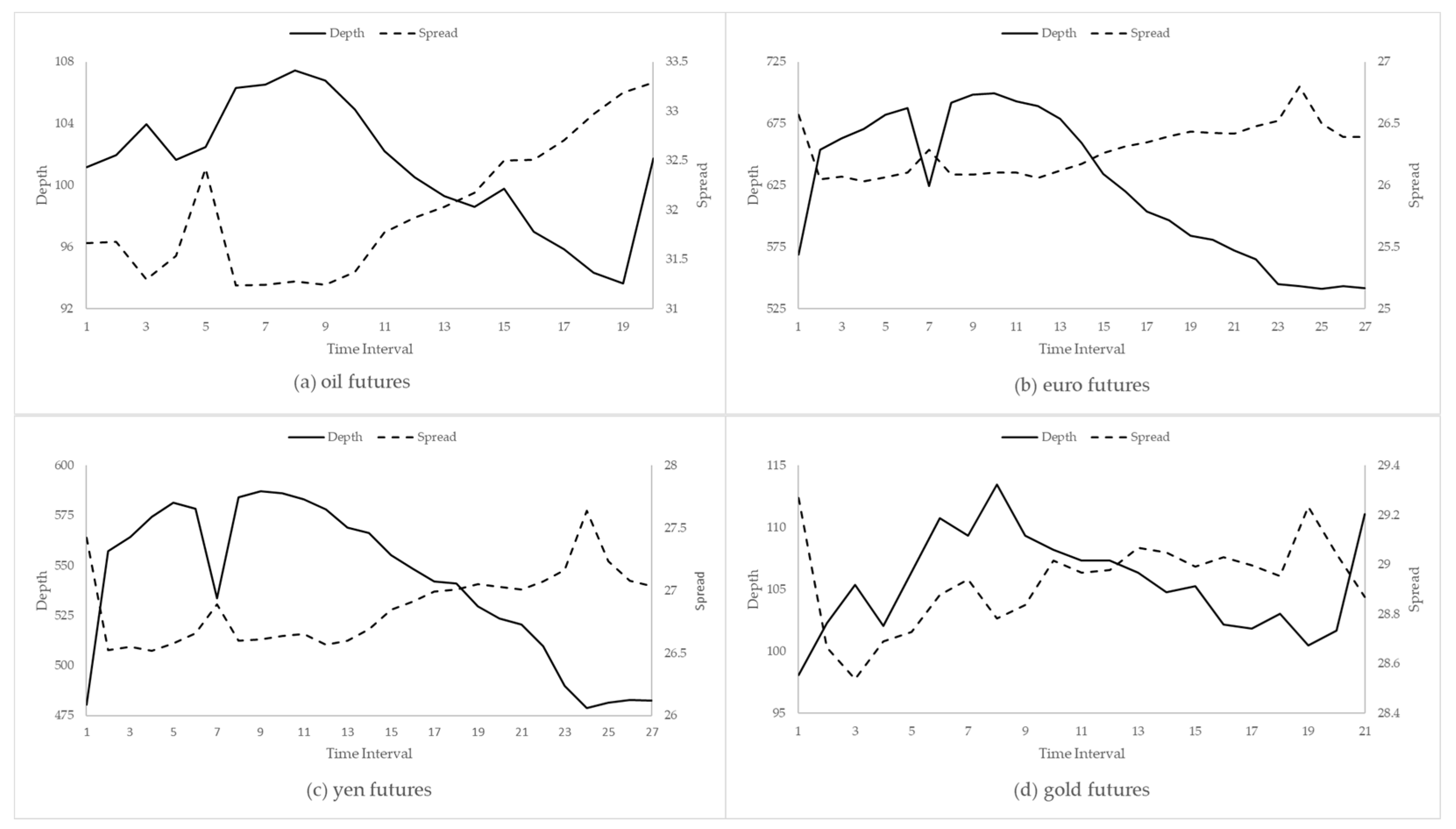
The intraday patterns of the depth and spread are pictured in Figure 1 for the oil, euro, yen, and gold futures.
The figure shows a reverse U-shaped pattern for the depth with decreased depth levels at the open and close of trading, relative to the middle of the day, for euro and yen futures. The depth pattern for oil and gold futures follows a reverse U-shape over the day with an increase in depth near the close of trading. In addition, the intraday pattern of the spread for these contracts appears U-shaped or increasing with large levels of total spread near the open and larger spreads near the close of trading, relative to the middle. The regression results for the intraday patterns of the depth and spread are presented in Table 3 for each futures contract.
The euro and yen futures in Table 3, Panel A, shows evidence of an inverse U-shaped pattern in depth, as indicated by the negative and significant coefficients on the dummy variables at the beginning and end of the day. The intraday depth pattern for oil futures in Panel A displays no evidence of elevated levels at the open but does support a decline in depth at the end of the trading day. Depth for the gold futures in Panel A shows lower levels at the open and near the close of the trading period as indicated by the negative and significant coefficients on Time1 and TimeN−1, but also shows a higher level relative to the middle for TimeN. Panel B in Table 3 shows an increasing bid–ask spread pattern over the day with negative and significant coefficients on the time dummy variables at the open and positive and significant coefficient on the time dummy variables at the close for oil and euro futures. The yen and gold futures in Panel B also show evidence of decreased spreads at the open of the trading day. Overall, the depth results exhibit an inverse U-shaped pattern for the day across the futures contracts, while the spread results display an increasing pattern over the day. Table 4 presents results for the intraday pattern of depth at each level in the five-deep limit order book.
In Table 4, the oil futures in Panel A and gold futures in Panel D show evidence of an increasing intraday pattern across the levels. The euro futures in Panel B and the yen futures in Panel C support an inverse U-shaped pattern in the depth as indicated by the negative and significant coefficients on the time dummy variables at the open and close of the day. Overall, the intraday depth patterns are consistent across the levels. Results for the intraday spread behavior for each of the five levels in the limit order book are presented in Table 5.
In Table 5, the coefficients on the time dummy variables indicate an increasing absolute bid–ask spread intraday pattern for oil and gold futures at each level. The intraday spread pattern is U-shaped for euro and yen futures at each level as indicated by the positive and significant coefficients on the time dummy variables at the open and close of the day.
3.3. Relation between Depth and Spread
Table 6 shows the results for the relation between depth and spread for the entire limit order book.
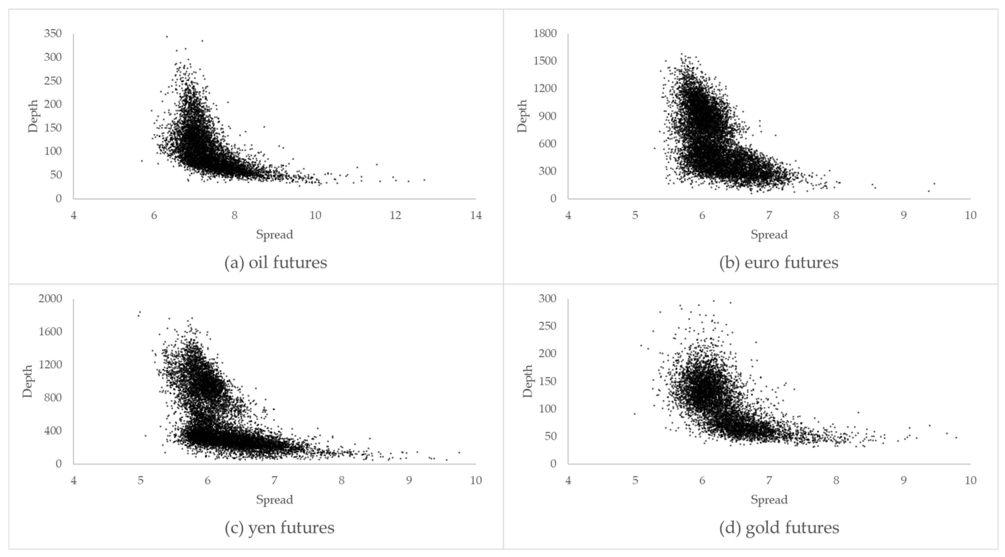
The main value of interest is the coefficient on the Spread variable. In Table 6, Panel A, the negative and statistically significant coefficient on the Spread supports an inverse relation between depth and spread across the four futures contracts. In Panel B, after controlling for the intraday variation and determinants of depth (including Volume, Level, and Volatility), the results show an inverse relation between depth and spread. Furthermore, the coefficient on the Volume is positive and significant, the coefficient on the Level is positive and significant, and the coefficient on the Volatility is negative and significant across the four contracts. Figure 2 depicts the inverse relationship between the depth and spread presented in Table 6.
Across all four futures contracts, larger (smaller) limit book depth is associated with smaller (larger) limit order book spread. In other words, liquid limit order books contain a large amount of volume available for trade. Table 7 displays results for the relation between depth and spread at each level in the limit order book.
In Panels A, B, C, and D of Table 7, the coefficient on the Spread variable at each level in the limit order book is negative and statistically significant. The main implication of these results is that the relation between depth and spread at each level is inverse or negative.
4. Conclusions
In conclusion, this paper provides results for the intraday behavior of the depth and spread, as well as their interaction, for four futures markets contracts that are widely traded around the world. The intraday behavior of the depth is generally found to have a systemic pattern consisting of an inverse U-shape. This finding is consistent with Lee et al. (1993), Brockman and Chung (2000), and Ahn and Cheung (1999), all of whom document an inverse U-shaped intraday depth pattern for stocks. We also find evidence to support an increasing intraday pattern for the spread.
Strong evidence to support an inverse relation between the depth and spread is documented, even after controlling for known explanatory factors. This finding is consistent both across the entire limit order book and at each individual level. The results mirror the general findings of Lee et al. (1993) for equities, that narrow depths are associated with large spreads. This association implies that limit order traders actively manage both price (spread) and quantity (depth) dimensions of liquidity. However, their conclusion only holds for the best level. The results of this paper, using five-deep depth data, extend their implication beyond stocks and beyond the best depth for futures markets, i.e., limit order traders actively manage spreads and depth along the five-deep limit order book.
The state of the entire limit book is essential for understanding the provision of liquidity, especially at times of excess demand and volatility. If large orders are submitted whose volume exceeds the depth available at the best level, these trades will transact at levels beyond the first. If the reduction of trading cost is a first-order concern, traders who execute large volumes would be interested in knowing the depth and spread relation for levels past the first. Large orders may walk up the book, and these orders pay an additional markup for the available depth beyond the amount offered at the best level. Future research avenues include exploring depth and liquidity interaction in limit order books with a larger level of transparency and consideration of the depth–spread relation for other futures markets.
Author Contributions
All authors contributed equally. All authors have read and agreed to the published version of the manuscript.
Funding
This research received no external funding.
Institutional Review Board Statement
Not applicable.
Informed Consent Statement
Not applicable.
Data Availability Statement
Restrictions apply to the availability of this data. Data were obtained from the CME Group and are available at https://datamine.cmegroup.com/#/, accessed on 20 October 2021.
Acknowledgments
We are grateful to Robert T. Daigler for poignant suggestions and insightful discussions. We thank Mark Holder and the CME Group for providing the futures market depth data.
Conflicts of Interest
The authors declare no conflict of interest.
| 1 | For ease of exposition, the light sweet crude oil (WTI) is referred to as “oil,” the euro/U.S. dollar total is referred to as the “euro,” and the yen/U.S. dollar futures is called the “yen.” |
| 2 | The date range for each contract is limited by the data provided to us by the CME Group. The end range of the data coincided with the period when the CME Group changed its data format from RLC to FIX/Fast format. |
| 3 | For example, there can be 30 depth updates in one second and only one depth update in another second. In order to sample the data at equal intervals, it is sampled every second. |
| 4 | To confirm that results are robust to the selection of the time interval, five-minute intervals are also employed. Similar results are obtained in the case of five-minute intervals and are available upon request. |
| 5 | The total spread is weighted by the percentage depth at each level for several reasons. Absence any weighting, the sum of absolute bid–ask spreads across each level becomes very noisy, especially in volatile and trending markets. In addition, the goal is to capture the size of the average difference between the bid and ask at different levels and this can be accomplished by measuring each spread as a percentage of the entire depth. |
| 6 | For ease of exposition, the total depth henceforth is referred to as “depth,” and the total spread is referred to as “spread.” |
| 7 |
References
- Ahn, Hee-Joon, and Yan-Leung Cheung. 1999. The intraday patterns of the spread and depth in a market without market makers: The stock exchange of Hong Kong. Pacific-Basin Finance Journal 7: 539–56. [Google Scholar] [CrossRef]
- Aidov, Alexandre, and Robert T. Daigler. 2015. Depth characteristics for the electronic futures limit order book. Journal of Futures Markets 35: 542–60. [Google Scholar] [CrossRef]
- Aitken, Michael, and Alex Frino. 1996. The determinants of market bid ask spreads on the Australian stock exchange: Cross-sectional analysis. Accounting & Finance 36: 51–63. [Google Scholar]
- Aitken, Michael, Niall Almeida, Frederick H. de B. Harris, and Thomas H. McInish. 2007. Liquidity supply in electronic markets. Journal of Financial Markets 10: 144–68. [Google Scholar] [CrossRef]
- Biais, Bruno, Pierre Hillion, and Chester Spatt. 1995. An empirical analysis of the limit order book and the order flow in the Paris bourse. The Journal of Finance 50: 1655–89. [Google Scholar] [CrossRef]
- Bouchaud, Jean-Philippe, Marc Mézard, and Marc Potters. 2002. Statistical properties of stock order books: Empirical results and models. Quantitative Finance 2: 251–56. [Google Scholar] [CrossRef]
- Brockman, Paul, and Dennis Y. Chung. 2000. An empirical investigation of trading on asymmetric information and heterogeneous prior beliefs. Journal of Empirical Finance 7: 417–54. [Google Scholar] [CrossRef]
- Cao, Charles, Oliver Hansch, and Xiaoxin Wang. 2009. The information content of an open limit-order book. Journal of Futures Markets 29: 16–41. [Google Scholar] [CrossRef]
- Chan, Kalok, Y. Peter Chung, and Herb Johnson. 1995. The intraday behavior of bid-ask spreads for NYSE stocks and CBOE options. The Journal of Financial and Quantitative Analysis 30: 329–46. [Google Scholar] [CrossRef]
- Chiu, Junmao, Huimin Chung, and George H. K. Wang. 2014. Intraday liquidity provision by trader types in a limit order market: Evidence from Taiwan index futures. Journal of Futures Markets 34: 145–72. [Google Scholar] [CrossRef]
- Ding, David K. 1999. The determinants of bid-ask spreads in the foreign exchange futures market: A microstructure analysis. Journal of Futures Markets 19: 307–24. [Google Scholar] [CrossRef]
- Frino, Alex, Andrew Lepone, and Grant Wearin. 2008. Intraday behavior of market depth in a competitive dealer market: A note. Journal of Futures Markets 28: 294–307. [Google Scholar] [CrossRef]
- Gwilym, Owain Ap, Mike Buckle, and Stephen H. Thomas. 1997. The intraday behavior of bid-ask spreads, returns, and volatility for FTSE-100 stock index options. The Journal of Derivatives 4: 20–32. [Google Scholar] [CrossRef]
- Hansen, Lars Peter. 1982. Large sample properties of generalized method of moments estimators. Econometrica 50: 1029–54. [Google Scholar] [CrossRef]
- Harris, Lawrence E. 1991. Liquidity, trading rules, and electronic trading systems. In Monograph Series in Finance and Economics. New York: New York University Salomon Center. [Google Scholar]
- Harris, Lawrence E. 1994. Minimum price variations, discrete bid-ask spreads, and quotation sizes. The Review of Financial Studies 7: 149–78. [Google Scholar] [CrossRef] [Green Version]
- Hautsch, Nikolaus, and Ruihong Huang. 2012. The market impact of a limit order. Journal of Economic Dynamics and Control 36: 501–22. [Google Scholar] [CrossRef] [Green Version]
- Lee, Charles M. C., Belinda Mucklow, and Mark J. Ready. 1993. Spreads, depths, and the impact of earnings information: An intraday analysis. The Review of Financial Studies 6: 345–74. [Google Scholar] [CrossRef]
- Newey, Whitney K., and Kenneth D. West. 1987. A simple, positive semi-definite, heteroskedasticity and autocorrelation consistent covariance matrix. Econometrica 55: 703–8. [Google Scholar] [CrossRef]
- Parlour, Christine A. 1998. Price dynamics in limit order markets. The Review of Financial Studies 11: 789–816. [Google Scholar] [CrossRef]
- Sheikh, Aamir M., and Ehud I. Ronn. 1994. A characterization of the daily and intraday behavior of returns on options. The Journal of Finance 49: 557–79. [Google Scholar] [CrossRef]
- Vo, Minh T. 2007. Limit orders and the intraday behavior of market liquidity: Evidence from the Toronto stock exchange. Global Finance Journal 17: 379–96. [Google Scholar] [CrossRef] [Green Version]
- Yura, Yoshihiro, Hideki Takayasu, Didier Sornette, and Misako Takayasu. 2014. Financial brownian particle in the layered order-book fluid and fluctuation-dissipation relations. Physical Review Letters 112: 1–5. [Google Scholar] [CrossRef] [PubMed] [Green Version]
Figure 1.
Intraday depth and spread behavior. This figure presents the intraday behavior of the depth and spread over the day using 15-min intervals. (a) Depicts oil futures, (b) depicts euro futures, (c) depicts yen futures, and (d) depicts gold futures. Depth is calculated as the sum of the depth available across all five levels. Spread is calculated as the sum of the depth-weighted spreads across all five levels.

Figure 2.
Scatterplot of depth and spread. This figure presents a scatterplot of the depth and spread using 15-min interval data. (a) Depicts oil futures, (b) depicts euro futures, (c) depicts yen futures, and (d) depicts gold futures. Depth is calculated as the sum of the depth available across all five levels. Spread is calculated as the sum of the depth-weighted spreads across all five levels.


Table 1.
Hours and dates.
| Futures Contract | Symbol | Hours | Date |
|---|---|---|---|
| Oil | CL | 08:00–13:30 | 01/02/2008–04/17/2009 |
| Euro | 6E | 07:20–14:00 | 01/03/2008–10/02/2009 |
| Yen | 6J | 07:20–14:00 | 01/03/2008–10/02/2009 |
| Gold | GC | 07:20–12:30 | 01/02/2008–04/17/2009 |
This table presents information about the time period and futures contracts used in this study. Symbol represents the CME Globex code for the futures contract. Hours represents electronic trading during the traditional floor trading session. Date represents the time span of the data employed in this study.
Table 2.
Summary statistics.
| Panel A: Oil | Mean | Median | Stan. Dev. | Skew. | Kurt. | 5th | 95th |
| Depth | 101.83 | 92.79 | 42.33 | 0.80 | 0.08 | 48.53 | 185.91 |
| Spread | 7.40 | 7.26 | 0.68 | 2.68 | 20.33 | 6.63 | 8.58 |
| Volume | 17,894.34 | 13,882.00 | 13,067.82 | 2.52 | 9.08 | 6265.00 | 45,489.00 |
| Level | 87.45 | 95.04 | 33.90 | −0.12 | −1.42 | 39.49 | 136.62 |
| Volatility | 0.18 | 0.15 | 0.13 | 3.40 | 18.50 | 0.06 | 0.40 |
| Panel B: Euro | Mean | Median | Stan. Dev. | Skew. | Kurt. | 5th | 95th |
| Depth | 640.25 | 601.37 | 298.48 | 0.21 | −1.17 | 226.45 | 1135.22 |
| Spread | 6.19 | 6.11 | 0.36 | 0.96 | 0.77 | 5.74 | 6.91 |
| Volume | 9123.99 | 7163.00 | 7328.55 | 2.51 | 11.59 | 2084.00 | 22,682.00 |
| Level | 14.19 | 14.18 | 0.99 | 0.05 | −1.12 | 12.67 | 15.72 |
| Volatility | 0.01 | 0.01 | 0.01 | 6.81 | 70.01 | 0.00 | 0.02 |
| Panel C: Yen | Mean | Median | Stan. Dev. | Skew. | Kurt. | 5th | 95th |
| Depth | 549.92 | 419.56 | 336.86 | 0.67 | −0.84 | 161.77 | 1188.86 |
| Spread | 6.20 | 6.10 | 0.45 | 1.23 | 2.20 | 5.65 | 7.07 |
| Volume | 4599.84 | 3546.00 | 3718.58 | 2.32 | 10.00 | 968.00 | 11,722.00 |
| Level | 0.01 | 0.01 | 0.00 | 0.04 | −1.13 | 0.01 | 0.01 |
| Volatility | 0.00 | 0.00 | 0.00 | 3.44 | 21.29 | 0.00 | 0.00 |
| Panel D: Gold | Mean | Median | Stan. Dev. | Skew. | Kurt. | 5th | 95th |
| Depth | 105.40 | 104.48 | 41.22 | 0.30 | −0.71 | 46.50 | 175.19 |
| Spread | 6.36 | 6.25 | 0.49 | 1.52 | 4.23 | 5.78 | 7.29 |
| Volume | 7084.21 | 5789.00 | 5076.28 | 2.58 | 12.15 | 1981.00 | 16,399.00 |
| Level | 88.21 | 89.25 | 6.28 | −0.72 | 0.12 | 74.72 | 97.15 |
| Volatility | 0.10 | 0.08 | 0.09 | 5.44 | 44.69 | 0.03 | 0.22 |
This table presents the summary statistics for the 15-min time intervals for each futures contract. Depth is calculated as the sum of the depth available across all five levels. Spread is calculated as the sum of the depth-weighted spreads across all five levels. Volume is computed as the sum of trade volume in each time interval. Level is represented by the mean trade price in each time interval. Volatility is defined by the standard deviation of trade prices in each time interval.
Table 3.
Intraday patterns of spread and depth.
| Panel A: Model 1 | Oil | Euro | Yen | Gold |
| Variables | Coeff. (p-Val.) | Coeff. (p-Val.) | Coeff. (p-Val.) | Coeff. (p-Val.) |
| Intercept | 102.107 (0.0000) | 648.640 (0.0000) | 558.853 (0.0000) | 105.786 (0.0000) |
| Time1 | −0.624 (0.3990) | −68.727 (0.0018) | −75.864 (0.0020) | −7.877 (0.0064) |
| Time2 | 0.291 (0.4508) | 14.752 (0.1730) | 1.399 (0.4697) | −3.416 (0.1020) |
| TimeN−1 | −8.833 (0.0038) | −95.244 (0.0005) | −78.138 (0.0018) | −4.256 (0.0572) |
| TimeN | 0.893 (0.3494) | −101.56 (0.0004) | −81.241 (0.0016) | 6.460 (0.0247) |
| Panel B: Model 2 | Oil | Euro | Yen | Gold |
| Variables | Coeff. (p-Val.) | Coeff. (p-Val.) | Coeff. (p-Val.) | Coeff. (p-Val.) |
| Intercept | 7.388 (0.0000) | 6.196 (0.0000) | 6.208 (0.0000) | 6.368 (0.0000) |
| Time1 | −0.078 (0.0376) | −0.103 (0.0008) | −0.041 (0.0659) | −0.063 (0.0391) |
| Time2 | −0.063 (0.0610) | −0.116 (0.0004) | −0.084 (0.0051) | −0.084 (0.0105) |
| TimeN−1 | 0.255 (0.0013) | 0.053 (0.0167) | 0.032 (0.1102) | 0.030 (0.1952) |
| TimeN | 0.154 (0.0106) | 0.011 (0.2843) | 0.000 (0.5000) | −0.083 (0.0250) |
This table presents the coefficient estimates for Model 1: and Model 2: . Depth is calculated as the sum of the depth available across all five levels. Spread is calculated as the sum of the depth-weighted spreads across all five levels. Time is a dummy variable for the time interval that takes a value of one or zero. Time1, Time2, TimeN−1, and TimeN, represent the first, second, second to last, and last time interval each day, respectively. Each regression is estimated using Hansen’s (1982) generalized method of moments (GMM) procedure along with the Newey and West (1987) correction. p-values are given in parenthesis.
Table 4.
Intraday patterns of depth at each level.
| Panel A: Oil | Level 1 | Level 2 | Level 3 | Level 4 | Level 5 |
| Variables | Coeff. (p-Val.) | Coeff. (p-Val.) | Coeff. (p-Val.) | Coeff. (p-Val.) | Coeff. (p-Val.) |
| Intercept | 10.241 (0.0000) | 16.263 (0.0000) | 22.134 (0.0000) | 27.226 (0.0000) | 30.919 (0.0000) |
| Time1 | −0.267 (0.0958) | −0.077 (0.8274) | −0.161 (0.7813) | −0.497 (0.5272) | −0.896 (0.3104) |
| Time2 | −0.291 (0.0619) | 0.046 (0.8932) | −0.003 (0.9964) | −0.112 (0.8872) | −0.813 (0.3466) |
| TimeN−1 | −0.004 (0.9794) | −1.407 (0.0000) | −2.281 (0.0000) | −2.353 (0.0009) | −1.730 (0.0300) |
| TimeN | 2.933 (0.0000) | 2.726 (0.0000) | 2.464 (0.0004) | 1.959 (0.0270) | 1.399 (0.1486) |
| Panel B: Euro | Level 1 | Level 2 | Level 3 | Level 4 | Level 5 |
| Variables | Coeff. (p-Val.) | Coeff. (p-Val.) | Coeff. (p-Val.) | Coeff. (p-Val.) | Coeff. (p-Val.) |
| Intercept | 43.819 (0.0000) | 114.447 (0.0000) | 164.574 (0.0000) | 173.778 (0.0000) | 162.100 (0.0000) |
| Time1 | −0.565 (0.6078) | −9.861 (0.0005) | −20.076 (0.0000) | −23.293 (0.0000) | −27.057 (0.0000) |
| Time2 | 4.494 (0.0001) | 5.745 (0.0574) | 2.725 (0.4879) | 2.512 (0.5078) | −5.780 (0.0629) |
| TimeN−1 | −6.285 (0.0000) | −19.839 (0.0000) | −25.448 (0.0000) | −26.164 (0.0000) | −17.563 (0.0000) |
| TimeN | −4.808 (0.0000) | −19.359 (0.0000) | −27.107 (0.0000) | −29.328 (0.0000) | −23.901 (0.0000) |
| Panel C: Yen | Level 1 | Level 2 | Level 3 | Level 4 | Level 5 |
| Variables | Coeff. (p-Val.) | Coeff. (p-Val.) | Coeff. (p-Val.) | Coeff. (p-Val.) | Coeff. (p-Val.) |
| Intercept | 40.053 (0.0000) | 104.107 (0.0000) | 148.393 (0.0000) | 146.843 (0.0000) | 124.395 (0.0000) |
| Time1 | −3.143 (0.0107) | −14.765 (0.0000) | −23.336 (0.0000) | −23.237 (0.0000) | −21.084 (0.0000) |
| Time2 | 2.059 (0.1410) | 1.072 (0.7709) | −0.772 (0.8714) | −0.981 (0.8191) | −3.698 (0.2664) |
| TimeN−1 | −4.889 (0.0000) | −14.737 (0.0001) | −21.841 (0.0000) | −21.024 (0.0000) | −12.972 (0.0000) |
| TimeN | −3.898 (0.0010) | −16.429 (0.0000) | −23.344 (0.0000) | −22.754 (0.0000) | −16.186 (0.0000) |
| Panel D: Gold | Level 1 | Level 2 | Level 3 | Level 4 | Level 5 |
| Variables | Coeff. (p-Val.) | Coeff. (p-Val.) | Coeff. (p-Val.) | Coeff. (p-Val.) | Coeff. (p-Val.) |
| Intercept | 13.098 (0.0000) | 20.717 (0.0000) | 23.838 (0.0000) | 25.166 (0.0000) | 27.292 (0.0000) |
| Time1 | 1.243 (0.0001) | −0.854 (0.0842) | −2.081 (0.0001) | −2.676 (0.0000) | −3.363 (0.0000) |
| Time2 | 0.152 (0.5765) | −0.468 (0.3274) | −0.930 (0.0892) | −0.774 (0.1871) | −1.048 (0.1040) |
| TimeN−1 | 0.073 (0.8305) | −0.631 (0.2488) | −0.690 (0.2817) | −0.751 (0.2467) | −0.387 (0.5680) |
| TimeN | 2.750 (0.0000) | 2.139 (0.0018) | 1.743 (0.0225) | 1.687 (0.0303) | 1.058 (0.2320) |
This table shows the coefficient estimates for the following model: . Depth is calculated as the sum of the bid and ask depth at each level. Time is a dummy variable for the time interval that takes a value of one or zero. Time1, Time2, TimeN−1, and TimeN, represent the first, second, second to last, and last time interval each day, respectively. Each regression is estimated using Hansen’s (1982) generalized method of moments (GMM) procedure along with the Newey and West (1987) correction. p-values are given in parenthesis.
Table 5.
Intraday patterns of spread at each level.
| Panel A: Oil | Level 1 | Level 2 | Level 3 | Level 4 | Level 5 |
| Variables | Coeff. (p-Val.) | Coeff. (p-Val.) | Coeff. (p-Val.) | Coeff. (p-Val.) | Coeff. (p-Val.) |
| Intercept | 2.191 (0.0000) | 4.365 (0.0000) | 6.417 (0.0000) | 8.443 (0.0000) | 10.461 (0.0000) |
| Time1 | −0.032 (0.2474) | −0.046 (0.2148) | −0.057 (0.1669) | −0.064 (0.1398) | −0.069 (0.1275) |
| Time2 | −0.024 (0.3859) | −0.042 (0.2579) | −0.053 (0.1952) | −0.060 (0.1616) | −0.066 (0.1414) |
| TimeN−1 | 0.157 (0.0000) | 0.250 (0.0000) | 0.283 (0.0000) | 0.301 (0.0000) | 0.320 (0.0000) |
| TimeN | 0.127 (0.0002) | 0.223 (0.0000) | 0.267 (0.0000) | 0.297 (0.0000) | 0.325 (0.0000) |
| Panel B: Euro | Level 1 | Level 2 | Level 3 | Level 4 | Level 5 |
| Variables | Coeff. (p-Val.) | Coeff. (p-Val.) | Coeff. (p-Val.) | Coeff. (p-Val.) | Coeff. (p-Val.) |
| Intercept | 1.251 (0.0000) | 3.254 (0.0000) | 5.255 (0.0000) | 7.256 (0.0000) | 9.257 (0.0000) |
| Time1 | 0.030 (0.0026) | 0.048 (0.0001) | 0.059 (0.0000) | 0.071 (0.0000) | 0.085 (0.0000) |
| Time2 | −0.042 (0.0000) | −0.044 (0.0000) | −0.044 (0.0000) | −0.045 (0.0000) | −0.047 (0.0000) |
| TimeN−1 | 0.023 (0.0104) | 0.023 (0.0136) | 0.022 (0.0170) | 0.022 (0.0217) | 0.022 (0.0249) |
| TimeN | 0.023 (0.0118) | 0.024 (0.0131) | 0.023 (0.0161) | 0.023 (0.0195) | 0.023 (0.0220) |
| Panel C: Yen | Level 1 | Level 2 | Level 3 | Level 4 | Level 5 |
| Variables | Coeff. (p-Val.) | Coeff. (p-Val.) | Coeff. (p-Val.) | Coeff. (p-Val.) | Coeff. (p-Val.) |
| Intercept | 1.362 (0.0000) | 3.368 (0.0000) | 5.372 (0.0000) | 7.376 (0.0000) | 9.382 (0.0000) |
| Time1 | 0.051 (0.0033) | 0.085 (0.0004) | 0.111 (0.0002) | 0.141 (0.0002) | 0.179 (0.0001) |
| Time2 | −0.055 (0.0000) | −0.059 (0.0000) | −0.062 (0.0000) | −0.066 (0.0000) | −0.072 (0.0000) |
| TimeN−1 | 0.036 (0.0159) | 0.037 (0.0262) | 0.037 (0.0416) | 0.038 (0.0561) | 0.046 (0.0489) |
| TimeN | 0.030 (0.0642) | 0.033 (0.0854) | 0.034 (0.1197) | 0.036 (0.1498) | 0.044 (0.1340) |
| Panel D: Gold | Level 1 | Level 2 | Level 3 | Level 4 | Level 5 |
| Variables | Coeff. (p-Val.) | Coeff. (p-Val.) | Coeff. (p-Val.) | Coeff. (p-Val.) | Coeff. (p-Val.) |
| Intercept | 1.714 (0.0000) | 3.787 (0.0000) | 5.807 (0.0000) | 7.817 (0.0000) | 9.825 (0.0000) |
| Time1 | −0.002 (0.9345) | 0.047 (0.1098) | 0.075 (0.0264) | 0.098 (0.0081) | 0.116 (0.0035) |
| Time2 | −0.060 (0.0017) | −0.057 (0.0267) | −0.056 (0.0484) | −0.056 (0.0630) | −0.056 (0.0691) |
| TimeN−1 | 0.024 (0.3022) | 0.030 (0.3309) | 0.036 (0.3064) | 0.042 (0.2777) | 0.052 (0.2376) |
| TimeN | −0.034 (0.1330) | −0.018 (0.5652) | −0.008 (0.8237) | 0.001 (0.9856) | 0.007 (0.8744) |
This table shows the coefficient estimates for the following model: . Spread is calculated as the absolute bid–ask spread, or ask price minus bid price, at each level. Time is a dummy variable for the time interval that takes a value of one or zero. Time1, Time2, TimeN−1, and TimeN, represent the first, second, second to last, and last time interval each day, respectively. Each regression is estimated using Hansen’s (1982) generalized method of moments (GMM) procedure along with the Newey and West (1987) correction. p-values are given in parenthesis.
Table 6.
Depth–spread relation.
| Panel A: Model 3 | Oil | Euro | Yen | Gold |
| Variables | Coeff. (p-Val.) | Coeff. (p-Val.) | Coeff. (p-Val.) | Coeff. (p-Val.) |
| Intercept | 361.089 (0.0000) | 3776.38 (0.0000) | 3312.76 (0.0000) | 444.490 (0.0000) |
| Spread | −35.054 (0.0000) | −504.79 (0.0000) | −443.61 (0.0000) | −53.185 (0.0000) |
| Time1 | −3.341 (0.0078) | −120.84 (0.0000) | −93.864 (0.0001) | −11.230 (0.0002) |
| Time2 | −1.934 (0.1671) | −43.666 (0.0039) | −35.821 (0.0164) | −7.865 (0.0012) |
| TimeN−1 | 0.109 (0.4732) | −68.329 (0.0004) | −64.006 (0.0009) | −2.676 (0.1027) |
| TimeN | 6.283 (0.0053) | −95.921 (0.0000) | −81.231 (0.0003) | 2.049 (0.1918) |
| Panel B: Model 4 | Oil | Euro | Yen | Gold |
| Variables | Coeff. (p-Val.) | Coeff. (p-Val.) | Coeff. (p-Val.) | Coeff. (p-Val.) |
| Intercept | 349.961 (0.0000) | −220.630 (0.0797) | 4599.47 (0.0000) | 329.926 (0.0000) |
| Spread | −35.647 (0.0000) | −245.44 (0.0000) | −178.15 (0.0000) | −46.794 (0.0000) |
| Time1 | −3.384 (0.0528) | −96.322 (0.0000) | −87.120 (0.0000) | −14.187 (0.0000) |
| Time2 | −2.430 (0.1046) | −26.633 (0.0091) | −32.173 (0.0075) | −9.885 (0.0001) |
| TimeN−1 | 0.445 (0.3966) | −72.275 (0.0000) | −57.626 (0.0001) | 0.223 (0.4497) |
| TimeN | 2.526 (0.1672) | −87.405 (0.0000) | −68.193 (0.0000) | 5.360 (0.0153) |
| Volume | 0.000 (0.0007) | 0.004 (0.0000) | 0.012 (0.0000) | 0.001 (0.0000) |
| Level | 0.240 (0.0000) | 154.104 (0.0000) | −291,173 (0.0000) | 0.762 (0.0001) |
| Volatility | −77.901 (0.0000) | −4333.8 (0.0003) | −9.26E6 (0.0000) | −29.177 (0.0310) |
This table presents the coefficient estimates for Model 3: and Model 4: . Depth is calculated as the sum of the depth available across all five levels. Spread is calculated as the sum of the depth-weighted spreads across all five levels. Volume is computed as the sum of trade volume in each time interval. Level is represented by the mean trade price in each time interval. Volatility is defined by the standard deviation of trade prices in each time interval. Time is a dummy variable for the time interval that takes a value of one or zero. Time1, Time2, TimeN−1, and TimeN, represent the first, second, second to last, and last time interval each day, respectively. Each regression is estimated using Hansen’s (1982) generalized method of moments (GMM) procedure along with the Newey and West (1987) correction. p-values are given in parenthesis.
Table 7.
Depth–spread relation at each level.
| Panel A: Oil | Level 1 | Level 2 | Level 3 | Level 4 | Level 5 |
| Variables | Coeff. (p-Val.) | Coeff. (p-Val.) | Coeff. (p-Val.) | Coeff. (p-Val.) | Coeff. (p-Val.) |
| Intercept | 16.054 (0.0000) | 41.965 (0.0000) | 76.297 (0.0000) | 112.825 (0.0000) | 139.610 (0.0000) |
| Spread | −4.105 (0.0000) | −6.577 (0.0000) | −9.305 (0.0000) | −10.953 (0.0000) | −10.933 (0.0000) |
| Time1 | −0.529 (0.0000) | −0.561 (0.0122) | −0.886 (0.0202) | −1.379 (0.0114) | −1.860 (0.0029) |
| Time2 | −0.430 (0.0000) | −0.303 (0.1641) | −0.600 (0.1191) | −0.905 (0.1003) | −1.583 (0.0086) |
| TimeN−1 | 0.332 (0.0109) | −0.192 (0.4158) | −0.102 (0.7874) | 0.544 (0.2884) | 0.399 (0.4987) |
| TimeN | 1.365 (0.0000) | 1.063 (0.0199) | 1.384 (0.0452) | 1.593 (0.0797) | 0.522 (0.6034) |
| Volume | 0.000 (0.0000) | 0.000 (0.0000) | 0.000 (0.0000) | 0.000 (0.0000) | 0.000 (0.0000) |
| Level | 0.022 (0.0000) | 0.018 (0.0000) | 0.048 (0.0000) | 0.068 (0.0000) | 0.068 (0.0000) |
| Volatility | −0.737 (0.3086) | −4.380 (0.0025) | −8.352 (0.0010) | −13.432 (0.0003) | −19.321 (0.0000) |
| Panel B: Euro | Level 1 | Level 2 | Level 3 | Level 4 | Level 5 |
| Variables | Coeff. (p-Val.) | Coeff. (p-Val.) | Coeff. (p-Val.) | Coeff. (p-Val.) | Coeff. (p-Val.) |
| Intercept | −78.185 (0.0000) | 20.844 (0.6749) | 277.847 (0.0156) | 422.225 (0.0052) | 462.937 (0.0037) |
| Spread | −42.234 (0.0000) | −113.05 (0.0000) | −140.95 (0.0000) | −117.81 (0.0000) | −87.411 (0.0000) |
| Time1 | −0.339 (0.6239) | −5.649 (0.0030) | −13.035 (0.0000) | −16.452 (0.0000) | −19.877 (0.0000) |
| Time2 | 0.379 (0.6045) | −2.426 (0.1993) | −7.351 (0.0027) | −7.138 (0.0044) | −10.660 (0.0000) |
| TimeN−1 | −3.461 (0.0000) | −14.733 (0.0000) | −19.369 (0.0000) | −20.286 (0.0000) | −17.791 (0.0000) |
| TimeN | −1.557 (0.0420) | −13.656 (0.0000) | −20.338 (0.0000) | −22.638 (0.0000) | −20.466 (0.0000) |
| Volume | 0.001 (0.0000) | 0.001 (0.0000) | 0.001 (0.0000) | 0.001 (0.0000) | 0.001 (0.0000) |
| Level | 12.101 (0.0000) | 32.280 (0.0000) | 43.969 (0.0000) | 42.431 (0.0000) | 35.335 (0.0000) |
| Volatility | −219.13 (0.0000) | −541.50 (0.0000) | −764.98 (0.0000) | −768.68 (0.0000) | −691.65 (0.0000) |
| Panel C: Yen | Level 1 | Level 2 | Level 3 | Level 4 | Level 5 |
| Variables | Coeff. (p-Val.) | Coeff. (p-Val.) | Coeff. (p-Val.) | Coeff. (p-Val.) | Coeff. (p-Val.) |
| Intercept | 298.940 (0.0000) | 972.961 (0.0000) | 1365.99 (0.0000) | 1257.23 (0.0000) | 1001.04 (0.0000) |
| Spread | −20.241 (0.0000) | −46.512 (0.0000) | −54.679 (0.0000) | −36.748 (0.0000) | −22.802 (0.0000) |
| Time1 | −2.740 (0.0013) | −12.004 (0.0000) | −18.070 (0.0000) | −19.040 (0.0000) | −19.310 (0.0000) |
| Time2 | −1.174 (0.2098) | −6.251 (0.0081) | −9.162 (0.0039) | −8.256 (0.0047) | −9.015 (0.0001) |
| TimeN−1 | −2.398 (0.0017) | −9.176 (0.0008) | −15.621 (0.0000) | −15.546 (0.0000) | −13.810 (0.0000) |
| TimeN | −1.668 (0.0376) | −11.416 (0.0000) | −17.830 (0.0000) | −17.816 (0.0000) | −15.656 (0.0000) |
| Volume | 0.001 (0.0000) | 0.003 (0.0000) | 0.003 (0.0000) | 0.003 (0.0000) | 0.003 (0.0000) |
| Level | −23,039 (0.0000) | −70,750 (0.0000) | −91,600 (0.0000) | −83,277 (0.0000) | −65,712 (0.0000) |
| Volatility | −931,044 (0.0000) | −2.12E6 (0.0000) | −2.65E6 (0.0000) | −2.46E6 (0.0000) | −1.95E6 (0.0000) |
| Panel D: Gold | Level 1 | Level 2 | Level 3 | Level 4 | Level 5 |
| Variables | Coeff. (p-Val.) | Coeff. (p-Val.) | Coeff. (p-Val.) | Coeff. (p-Val.) | Coeff. (p-Val.) |
| Intercept | 21.360 (0.0000) | 57.304 (0.0000) | 85.706 (0.0000) | 99.060 (0.0000) | 95.542 (0.0000) |
| Spread | −7.952 (0.0000) | −11.758 (0.0000) | −11.906 (0.0000) | −10.941 (0.0000) | −9.539 (0.0000) |
| Time1 | 0.493 (0.0337) | −1.250 (0.0007) | −2.365 (0.0000) | −2.748 (0.0000) | −2.934 (0.0000) |
| Time2 | −0.863 (0.0000) | −1.833 (0.0000) | −2.462 (0.0000) | −2.221 (0.0000) | −1.964 (0.0001) |
| TimeN−1 | 0.940 (0.0005) | 0.593 (0.1537) | 0.822 (0.1006) | 0.762 (0.1472) | 1.121 (0.0471) |
| TimeN | 3.118 (0.0000) | 2.743 (0.0000) | 2.659 (0.0000) | 2.680 (0.0000) | 2.855 (0.0002) |
| Volume | 0.000 (0.0000) | 0.000 (0.0000) | 0.000 (0.0000) | 0.000 (0.0000) | 0.000 (0.0000) |
| Level | 0.042 (0.0005) | 0.066 (0.0049) | 0.052 (0.0794) | 0.102 (0.0022) | 0.253 (0.0000) |
| Volatility | −0.966 (0.4134) | −2.312 (0.3125) | −2.905 (0.2972) | −2.219 (0.4804) | −5.678 (0.1209) |
This table presents the coefficient estimates for the following model: . Depth is calculated as the sum of the bid and ask depth at each level. Spread is calculated as the absolute bid–ask spread, or ask price minus bid price, at each level. Volume is computed as the sum of trade volume in each time interval. Level is represented by the mean trade price in each time interval. Volatility is defined by the standard deviation of trade prices in each time interval. Time is a dummy variable for the time interval that takes a value of one or zero. Time1, Time2, TimeN−1, and TimeN, represent the first, second, second to last, and last time interval each day, respectively. Each regression is estimated using Hansen’s (1982) generalized method of moments (GMM) procedure along with the Newey and West (1987) correction. p-values are given in parenthesis.
Publisher’s Note: MDPI stays neutral with regard to jurisdictional claims in published maps and institutional affiliations. |
© 2021 by the authors. Licensee MDPI, Basel, Switzerland. This article is an open access article distributed under the terms and conditions of the Creative Commons Attribution (CC BY) license (https://creativecommons.org/licenses/by/4.0/).
Share and Cite
MDPI and ACS Style
Aidov, A.; Lobanova, O. The Relation between Intraday Limit Order Book Depth and Spread. Int. J. Financial Stud. 2021, 9, 60. https://0-doi-org.brum.beds.ac.uk/10.3390/ijfs9040060
AMA Style
Aidov A, Lobanova O. The Relation between Intraday Limit Order Book Depth and Spread. International Journal of Financial Studies. 2021; 9(4):60. https://0-doi-org.brum.beds.ac.uk/10.3390/ijfs9040060
Chicago/Turabian StyleAidov, Alexandre, and Olesya Lobanova. 2021. "The Relation between Intraday Limit Order Book Depth and Spread" International Journal of Financial Studies 9, no. 4: 60. https://0-doi-org.brum.beds.ac.uk/10.3390/ijfs9040060
Note that from the first issue of 2016, this journal uses article numbers instead of page numbers. See further details here.