Article

A Refined Lines/Regions and Lines/Lines Topological Relations Model Based on Whole-Whole Objects Intersection Components

1
School of Geosciences and Info-Physics, Central South University, Changsha 410083, China
2
Key Laboratory of Metallogenic Prediction of Nonferrous Metals and Geological Environment Monitoring Ministry, Central South University, Ministry of Education, Changsha 410083, China
*
Author to whom correspondence should be addressed.
ISPRS Int. J. Geo-Inf. 2021, 10(1), 15; https://0-doi-org.brum.beds.ac.uk/10.3390/ijgi10010015
Submission received: 13 November 2020 / Revised: 25 December 2020 / Accepted: 31 December 2020 / Published: 6 January 2021
(This article belongs to the Special Issue Geodata Science and Spatial Analysis in Urban Studies)

Abstract

:
Refined topological relations play an important role in spatial database quality control. Currently, there is no unified and reasonable method to represent refined line/region and line/line topological relations in two-dimensional (2D) space. In addition, the existing independent line/region and line/line models have some drawbacks such as incomplete type discrimination and too many topological invariants. In this paper, a refined line/region and line/line topological relations are represented uniformly by the sequence, dimension, and topological type of the intersection components. To make the relevant definitions conform to the traditional cognitions in 2D Euclidean space, the (simple) spatial object is defined based on manifold topology, and the spatial intersection components are defined based on the whole-whole object intersection set. Then the topological invariant of node degree is introduced, and the adjacent point kinds (e.g., “Null”, “On”, “In”, and “Out”) are defined to distinguish the intersection component types. Excluding impossible and symmetrical types, 29 types of intersection-lines (including 21 between lines/regions and 8 between lines/lines), and 6 types of intersection-points (including 2 between lines/regions and 4 between lines/lines) are classified. On this basis, a node degree-based whole-whole object intersection sets (N-WWIS) model for refined line/region and line/line topological relations is presented, and it can be combined with the Euler number-based whole object intersection and difference (E-WID) model (coarse level) to form a hierarchical representation method of topological relations. Furthermore, a prototype system based on the N-WWIS model for automatic topological integrity checking is developed and some evaluation experiments are conducted with OpenStreetMap (OSM) data is presented based on the classification of intersection components. The experimental results show that the N-WWIS model will enable the geographic information systems (GIS) community to develop automated topological conflict checking and dealing tools for spatial data updates and quality control.

1. Introduction

Lines and regions are very important spatial objects in two-dimensional (2D) geographic information systems (GIS). The topological relations of lines/regions and lines/lines also play an important role in spatial data organization, queries, updates, and quality control. For nearly thirty years, some formal models that are suitable for representing the topological relations about lines/regions and lines/lines in 2D space have been explored or developed. The best-known models are the four-intersection (4I) model [1] and the nine-intersection (9I) model [2], which aim to describe the basic topological relations, such as disjoint, meet, overlap, cover, equal, and inside. However, both the 4I and 9I models distinguish only the content of the intersections, which leads to their weak ability to distinguish the topological relations of line/region and line/line. For example, only the 11, 19 line/region and the 12, 33 line/line topological relations can be distinguished by the 4I and 9I models, respectively [3].
Subsequently, a number of extended models based on the 4I and 9I models have been proposed to distinguish more topological details, such as the dimension extended 9-intersection model (DE+9IM) [4], the Voronoi-based 9-intersection model [5], and the 27-intersection model [6]. Furthermore, some improved models that can distinguish only line/region topological relations have been proposed to identify more topological details, such as the modeling conceptual neighborhoods of topological line-region relations [7], the 9+-intersection model for directed line segments and regions [8], the directed polyline–polygon model [9], and the directed line–directed region model [10]. In addition to these above decomposition-based models [11], some scholars have developed different topological relation models from the perspective of the spatial object as a whole, such as the RCC (region connection calculus) model [12,13], the Voronoi-based spatial algebra model [14], and the Euler number-based whole object intersection and difference (E-WID) model [15]. Among them, the best performance is the E-WID model, which has a strict theory, few set operations and strong distinguishing ability.
However, although the distinguishing ability of some of the above models has improved compared with the abilities of 4I and 9I, these models are also coarse, i.e., they represent only coarse relations. These models describe only the overall topological properties of the intersections (or differences), such as content, dimension, Euler number, etc., and thus, some of their description results are ambiguous. In other words, some different relations, especially the refined relations that have multiple intersection components, have the same description results. In some practical GIS applications, the representation and calculation of refined topological relations, especially the sequence, dimension, and topological type of each intersection (or difference) component, are very important. For example, in line/region and line/line topological conflict detection and processing for OpenStreetMap (OSM) data, the involved objects are those with non-disjoint relations, e.g., cross, meet, inside, etc. These non-disjoint relations may have two or more intersection components. As shown in Figure 1a, the volunteer’s trajectory (line) L1 has three one-dimensional intersections (i1, i2, and i3) with the same lake (region) R1. Similarly, in Figure 1b, trajectory line L2 has three intersection components with trajectory line L3, including two one-dimensional intersections (i4 and i6) and one zero-dimensional intersection (i5). These relations with multiple intersection components must be addressed one-by-one according to their refined topological types. Therefore, it is necessary to study the representation and calculation of the line/region and line/line refined topological relations, especially the complete classification of the topological types of each intersection component.
For the line/region at a refined level, the LRBIS (intersections set between line and region boundary) method proposed by Deng [16] is representative at present. In this method, the line-region relations are classified into 16 types of basic relations (including 1 disjoint and 15 non-disjoint relations) based on the invariants of dimension and local order, and the compound relations are decomposed into and described by a combination of a finite number of basic intersection relations. However, the definition of the intersection component in this method is not based on the whole line and whole region intersection but is based on the intersection between the whole line and the boundary of the region. Therefore, its intersection components do not follow people’s cognitive habits well, and some actual types of one-dimensional intersections between the line and region interior are omitted. For example, this method defines only three cross types (see Figure 2a–c), while the other cross types that exist (Figure 2d,e) are not defined. In other words, the LRBIS method is incomplete.
For the refined relations between lines/lines, the existing representative method was proposed by Clementini and Felice [17]. In the method, the dimension, intersection type, collinearity sense, and link orientation of the intersection components and their sequence are used to describe the refined relations. Although it also describes the type of intersection component, it focuses more on the overall topological details of lines/lines, leading to the introduction of more topological invariants that are parallel to the type of intersection component, and the description becomes complicated.
At present, there are a few other studies on the refined relations of line/region and line/line, such as the detailed model of topological and metric relations between line and region [18] and the line/line compound relation model by using the basic relations [19]. However, these methods are either still incomplete or have very complex descriptions. For example, only seven types of detailed line segments are used to describe the refined topological relations between lines/region in Reference [18], and multi-level and multi-description factors are used to describe the refined line/line relations in Reference [19]. Furthermore, although the line/region and the line/line both have and only have one-dimensional and zero-dimensional intersection components, there is currently no unified method to represent their refined relations. Therefore, the reasonable (complete and concise) and unified representation of the line/region and line/line intersection components is still an open issue in the GIS community. It is necessary to introduce an effective, concise, and unified framework for describing the line/region and line/line refined relations.
In Reference [2], Zhou et al. proposed a hierarchical description and calculation method of topological relations between two regions in 2D space. In this method, the coarse relations are represented by the E-WID model, and the refined relations are mainly represented by the Euler number-based whole-whole intersection sets (E-WWIS) model. Although some extremely complex refined relations need to be distinguished in combination with the E-WWIS and boundary-boundary intersection sets (BBIS) [20] models, the E-WWIS model has performed well in practical applications. Furthermore, the E-WWIS model is based on the whole object intersection and has a reasonable description framework. The model uses the sequence, dimension, and topological type of the intersection component to represent the refined relations, which is concise and consistent with cognitive habits. Therefore, this paper will also use the original framework of the E-WWIS model to represent the refined relations of the line/region. However, although the Euler number performs well in the discrimination of 2D intersections, it does not work well in the one-dimensional and zero-dimensional intersections. Therefore, new topological invariants should be introduced instead of Euler numbers in the E-WWIS model for the discrimination of the types of one-dimensional and zero-dimensional intersection components between lines/regions (and lines/lines). After analyzing the characteristics of the intersection components, the topological invariants of node degree and adjacent point kinds are introduced and defined, and they are used to identify the types of intersection-lines and intersection-points; thus, a node degree-based whole-whole intersection sets (N-WWIS) model is produced for the refined topology between lines/regions (and lines/lines).
The remainder of the paper is structured as follows. In Section 2, the simple spatial objects in 2D space and the line/region (and line/line) intersection components are defined, and the node degree is introduced. In Section 3, the types of intersection components are classified using node degree and adjacent point kinds. The hierarchical representation of line/region and line/line topological relations based on the E-WID (coarse level) and N-WWIS (refined level) models are discussed in Section 4. Application and experimental tests in automatic topological integrity checking are presented in Section 5. The conclusions and discussion are presented in Section 6.

2. Definition of the Intersection Component and Introduction of the Node Degree

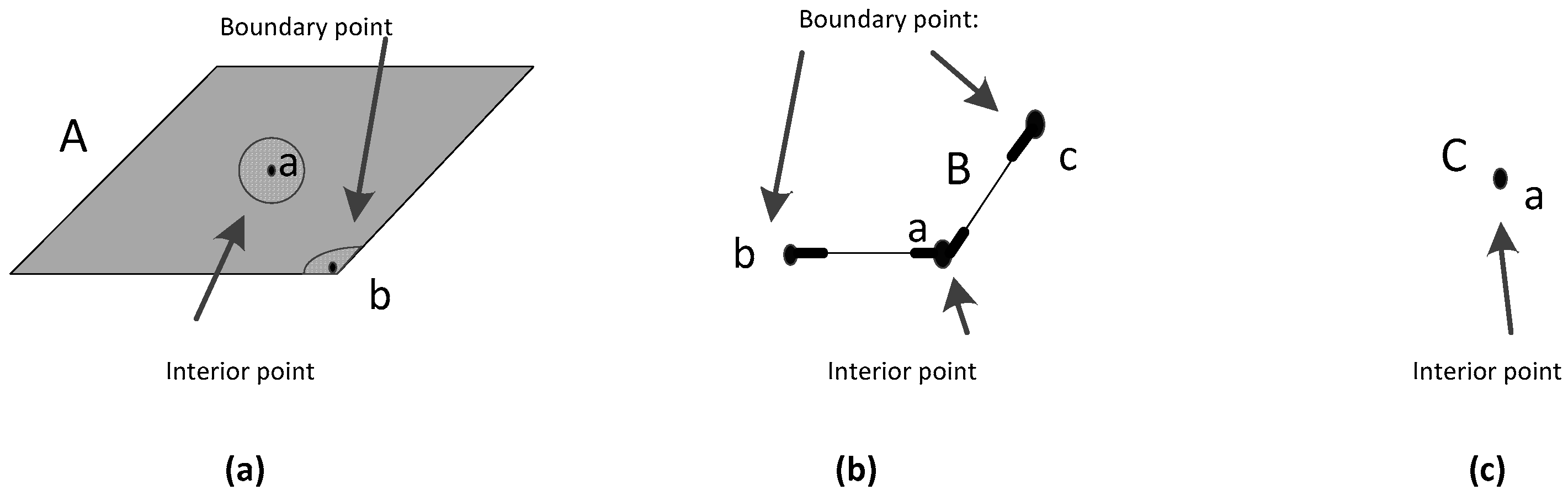
2.1. The Definition of a Simple Spatial Object

A good definition of spatial objects is an important basis for the effective description and discrimination of topological relations. In the GIS community, spatial objects are generally considered to be subsets of Euclidean space, and their topological definitions of “interior” and “boundary” are usually based on point-set topology. According to the point-set topology in Euclidean space, lines and points have boundaries but no interior in 2D space [21,22]. However, according to the traditional definition and cognition, both lines and points have interiors in 2D space [4,5,6,7,23]. Therefore, to avoid the conflict between the theoretical basis and traditional definition, spatial objects are regarded as manifolds embedded in 2D space, and their topological definitions are based on manifold topology. Manifolds and their boundary and interior are defined as follows [24,25].
“Definition 2.1” (Manifold): Let Rn be an n-dimensional Euclidean space, X is a locally Euclidean space of dimension n, and Hn = {(x1, x2, …, xn) ∈ Rn, n ≥ 0} (half space). If each point in X has a neighborhood homeomorphic to Rn, then X is an n-manifold (without boundary); if each point in X has a neighborhood either homeomorphic to Rn or homeomorphic to Hn, then X is an n-manifold with boundary. If a neighborhood of point p in X is homeomorphic to Rn, then p is called an interior point of X, and the set of all interior points of X is called the interior (X°) of X. If any neighborhood of point p in X is homeomorphic to Hn, then p is called a boundary point of X, and the set of all boundary points of X is called the boundary (∂A) of X.
Notably, a manifold itself is a topological space (local Euclidean space), so its neighborhood is only related to itself and is independent of the Euclidean space in which it is embedded, meaning that the definitions of the interior and boundary points in a manifold are also independent of the space in which the manifold is embedded (see Definition 2.1), which is different from the definitions using the point-set topology in Euclidean space. As shown in Figure 3, the region (Figure 3a), the line (Figure 3b), and the point (Figure 3c) all have interior points in R2, which is consistent with traditional definitions and cognitive habits. In addition, because a manifold is a special topological space, it also has some of its topological properties, such as whether it is compact, connected, orientable, etc. Further, manifolds are not self-intersecting or touching and homogeneous (same dimension). According to the geometric characteristics of common objects in the spatial database, the (simple) spatial objects in 2D space are defined as follows in this paper.
“Definition 2.2” (Spatial objects): A spatial object is a connected, compact and orientable n-manifold (0 ≤ n ≤ 2), which can be embedded in 2D space. A simple region is a two-manifold with one connected interior and one connected boundary. A simple line is a one-manifold with one connected interior and two separate boundaries. A simple point is a zero-manifold with a connected interior but no boundary.
As shown in Figure 3, the geometry of a simple region corresponds to a polygon, and its boundary is a closed curve (Figure 3a). The geometry of a simple line corresponds to a polyline, and its boundaries are two separate endpoints (Figure 3b). The geometry of a simple point corresponds to an isolated point and has no boundary (Figure 3c).

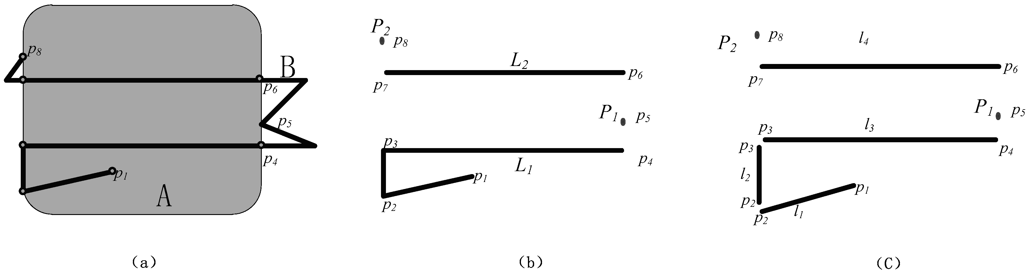
2.2. The Definition of Intersection Components

For the description of the refined relations, the existing models are mainly based on the sequence, dimension, and topological properties (topological type) of the intersection components. In refined models, such as E-WWIS, the components are obtained based on the whole-whole object intersection. Therefore, to represent and calculate the refined line/region and line/line relations, their intersection components first need to be well defined.
The concept of components is derived from topology. The topological components of any set X form a maximal connected subset (path-connected) of X: these components are disjoint and nonempty, and their union is the whole set X [24,26]. In the GIS community, the properties of topological components are usually directly used to define the intersection or difference components between spatial objects [20,27]. However, there are still some differences between spatial components and topological components. For example, in the spatial database, a spatial component must contain its proper boundaries [2,28], whereas a topological component may not (similar to an open disk). Furthermore, even if a topological component is appropriate in itself, some of them must be further subdivided to meet the actual needs of the applications and people’s cognitive habits.
As shown in Figure 4b, the intersection set of region A and line B has four maximal connected subsets (topological components), namely, L1 (p1p2p3p4), L2 (p6p7), P1 (p5), and P2 (p8). Among them, P1 and P2 are zero-dimensional intersections because they are both simply isolated points, so they do not need to be subdivided. L1 and L2 are one-dimensional intersections, where L2 does not need to be subdivided because its interior points are all in the interior of region A, whereas L1 is relatively complex, and its interior points do not have the same topological property in region A. For example, points between line segments l1 (p1p2) and l3(p3p3) are inside A, while points between line segments l2(p2p3) are on the boundary of region A. Therefore, even though intersection-line L1 is connected, it is more reasonable to break at points p1 and p2, which is also more in line with people’s cognitive habits. Furthermore, if we assume that region A is a lake, line B is a road shaped by the volunteer’s trajectory. Then, l1 (p1p2) may be a trail extending in the lake or a wrong trajectory segment, l2 (p2p3) maybe a road along the lake, and l3 (p3p3) may be a bridge across the lake. Therefore, in practical applications, the intersection-line L1 also needs to be subdivided.
According to the definition of topological components and the characteristics of GIS spatial data, the spatial intersection components of line/region and line/line are defined as follows:
“Definition 2.3” (Spatial intersection component): Let A be a region or a line and B be a line; let I be a maximal connected subset of AB. If I is zero-dimensional, then I is an intersection-point of AB; if I is one-dimensional, assume that the interior of segment l is a maximal connected subset of I or ∂AI, and l is an intersection-line of AB and I = U i = 1 n li (i > 1).
Based on Definition 2.3, there are six spatial intersection components between region A and line B in Figure 4, including four intersection-lines (l1, l2, l3, and l4) and two intersection-points (P1 and P2), as shown in Figure 4c. Among them, the intersection-lines l1, l2, and l3 are subdivided by the one-dimensional topological component L1 (Figure 4b). In addition, it should be noted that the intersection-line in Definition 2.3 contains boundaries; that is, their topologies are equal to a polyline with two endpoints shown in Figure 3. It should be noted that to simplify the expression, the term “intersection component” (e.g., “intersection-line” and “intersection-point”) used in this article refers specifically to the spatial intersection component (e.g., “spatial intersection-line” and “spatial intersection-point”) if there is no “topological” modifier.

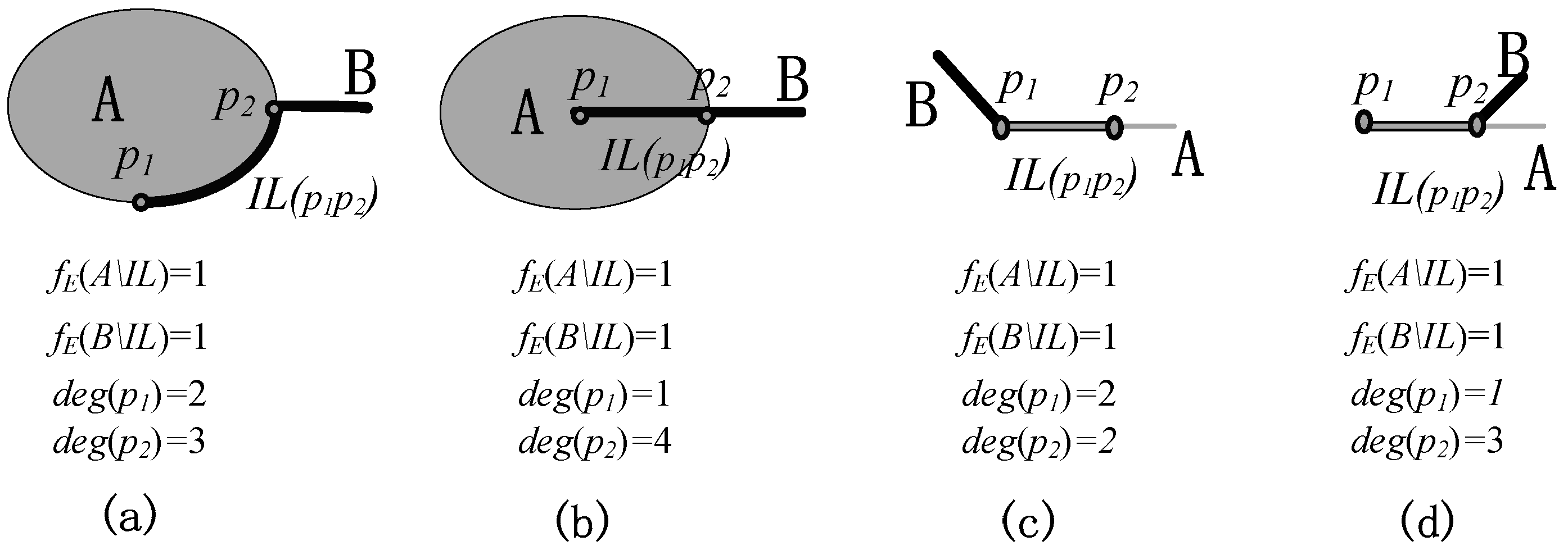
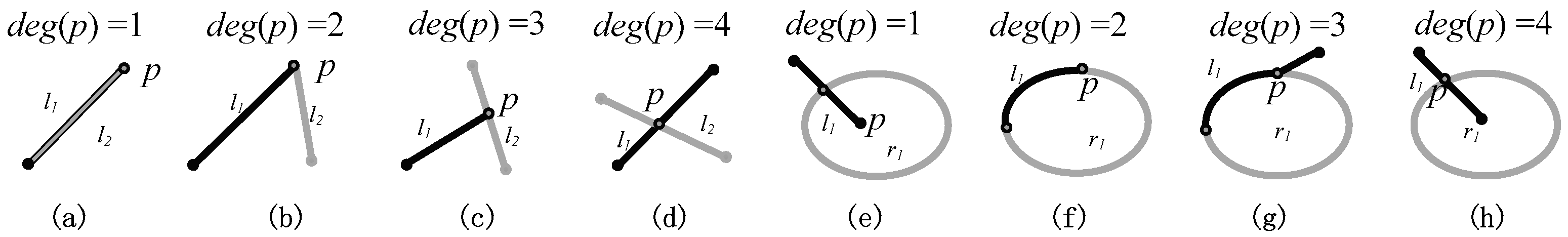
2.3. Introduction of the Node Degree

The basic framework of the E-WWIS model [2] can also be used to represent the refined relations of regions/regions with multiple intersections (including single intersections), as shown in Equation (1), where ‘Ni (1 ≤ im)’, ‘di’ and ‘ti’ denote the topological sequence, dimension and type of the corresponding intersection sets (components), respectively.
R (A, B) = <N1 (d1, t1), N2 (d2, t2),…, Nm (dm, tm)>
Among the three topological invariants of sequence, dimension, and type in the E-WWIS model, the most critical is the topological type, which represents the comprehensive configuration of the topological invariants of the intersection component except for the dimension and sequence. Therefore, the classification of intersection component (set) types is the key issue in the E-WWIS model. For the 2D intersection, their types are distinguished by the Euler numbers [29] of the difference between the two regions and the intersection component, i.e., let “IR” denote the intersection component, and the 2D intersection type is distinguished by fE (A\IR) and fE (B\IR) [2].
Although the framework of the E-WWIS model is also suitable for describing line/region and line/line refined relations with multi-intersections, some refined one-dimensional intersection (intersection-line) types of line/region and line/line cannot be distinguished by relying solely on the “Euler number”. For example, let “IL” denote intersection-line l; in Figure 5, region (or line) A intersects line B at segment l (p1p2). In Figure 5a,b, the values of fE (A\IL) and fE (B\IL) are the same. However, the topological types of the two intersecting lines are different, in Figure 5a, the intersection-line l is completely on the boundary of region A, and in Figure 5b intersection-line l is inside region A. Similarly, the intersection-line types between two lines in Figure 5c,d are different, but their values of fE (A\IL) and fE (B\IL) are the same.
Figure 5a–d differ in the number of edges incident to the endpoints of the intersection-lines. In topology and graph theory, a criterion that was used to settle the Königsberg Bridge Problem by Euler in the 18th century [30], is known as the “degree of point” [31,32]. The degree of a point is the number of edges incident to the vertex. It is assumed that the degree of a vertex p in a graph is denoted deg (p); then, point p is isolated if deg (p) = 0 or is an endpoint if deg (p) = 1 (Frank, 1969). Because the topological relation is based on the binary spatial objects, the node degree calculated in this paper is the node degree of a certain point in the union of two spatial objects, and when the object is a region, it is treated as its boundary only (excluding its interior). For example, when two lines are equal, then the degree of nodes at their endpoints is one (Figure 6a); when two lines meet at their endpoints, the degree of their intersection-point is two (Figure 6b); when one of a line’s endpoints meets at the interior of the other line, the degree of their intersection-point is three (Figure 6c); when two lines intersect at their interior, the degree of their intersection-point is four (Figure 6d). For a line and a region, if the endpoint of the line is inside of the region, then its degree is one (Figure 6e); if the endpoint of the line is on the boundary of the region, then its degree is two (Figure 6f); if one part of the line is on the boundary of the region and the other part is not, then the degree of the point where the topological properties change is three (Figure 6g); If a point is an intersection-point of the line and the boundary of the region, then its degree is four (Figure 6h).
For the intersection-lines of line/region and line/line, even though the degree of their interior points are all two, there are four different cases of the degree of their endpoints, including four possible values, i.e., {1,2,3,4}. In Figure 5a, the degree of p1 is two and the degree of p2 is three, while in Figure 5b, the degree of p1 is one, and the degree of p2 is four; in Figure 5c, the degrees of p1 and p2 are both two, while in Figure 5d, the degree of p1 is one and the degree of p2 is three. The node degree, i.e., “degree of point”, can be used to distinguish different types of intersection-lines in Figure 5.
It is clear that the node degree is a topological invariant, and its ability to distinguish intersecting lines is better than that of the Euler number. In addition, because the degree of the intersection-point can also work well in the discrimination of intersection-points, the node degree is used to distinguish both types of intersection-points and intersection-lines between lines/regions and lines/lines. Therefore, a N-WWIS model can be proposed for representing the refined line/region and line/line relations.

3. Classification of Intersection-Lines and Intersection-Points Based on Node Degrees

3.1. Classification of the Intersection-Line between the Line and Region

As mentioned above, the intersection-line of the line/region can be distinguished using the degrees of the two endpoints of the intersection-line (i.e., p1 and p2 in Figure 7). Since there are four possible values for the degree of each endpoint, there are theoretically 16 (4 × 4) possible combinations. Excluding the impossible and symmetric values, we can obtain 8 types of possible intersection component types (i.e., the types actually exist in R2), whose node degrees are (1,1), (1,3), (1,4), (2,2), (2,3), (3,3), (3,4), and (4,4), as shown in Figure 7.
This method can fully distinguish the types of intersection-lines whose degree values of endpoints are all one or two. However, other types of intersection-lines cannot be distinguished by only degree values. For example, two pairs of different intersection-lines with degree values of three or four are shown in Figure 8. The degree values of the endpoints of the intersection-line in Figure 8a,b are both equal (1,3), and the degrees in Figure 8c,d equal (1,4).
By analyzing the two couple relations in Figure 8, we found that the main difference between them lies in the topological properties of endpoint p2 of the intersection-lines. Endpoint p2 in Figure 8a is the boundary point of line B, while in Figure 8b, line B has one segment following endpoint p2 and is on the boundary of region B. In Figure 8c, the following segment of endpoint p2 in line B is inside region A, while in Figure 8d, it is outside region A. The topological properties of the endpoints of the intersection-line are not only their node degrees; they are also related to the kinds of their adjacent points. The definition of adjacent points is described as follows.
“Definition 3.1” (Adjacent point): Let L be an intersection component between region (or line) A and line B. If L is an intersection-point, let point p be L; if L is an intersection-line, let point p be an endpoint of L. Given an arbitrarily small real number r, and let point A(p) be a point belonging to line B but not to L; if the distance between point A(p) and p is r, then the point A(p) is the adjacent point of p. If the adjacent point of p does not exist, it is named as Null. If the point is on the boundary of A, it is named as On. If the point is inside A, it is named as In. If the point is outside A, it is named as Out.
The Definition 3.1 applies not only to intersection-lines but also to intersection-points of lines/regions and lines/lines. The endpoint of the intersection-line contains one adjacent point at most, of which there are four possible kinds: Null, On, In, and Out, as shown in Figure 8. By combining the node degrees and adjacent point kinds of the endpoints, the four types of intersection-lines in Figure 8 can be distinguished.
By combining the degree of nodes (1,2,3,4) and the adjacent point kinds (Null, On, In, and Out), our model can distinguish the different 256 (4 × 4 × 4 × 4) types of intersection-lines between line/regions in theory. However, only a few of them (possible types) actually exist in R2. Since the node degree values of the intersection-line endpoints only exist a total of 16 combined values (only 10 asymmetric), the possible types can be searched one by one based on these combined values and their corresponding possible adjacent point kinds. In fact, 21 types of possible and asymmetric intersection-lines are classified and found by using this method, as shown in Figure 9. It should be noted that the node degree has a higher priority than the adjacent point kinds, so the description of adjacent point kinds is sometimes ignored when it is not necessary.
The corresponding proofs of 21 types of intersection-lines between lines and regions are as follows.
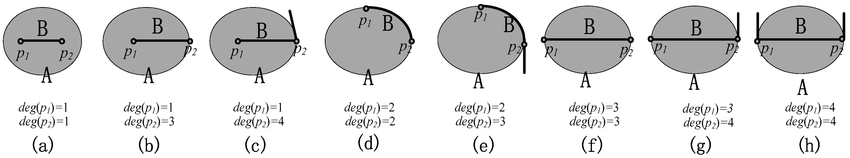
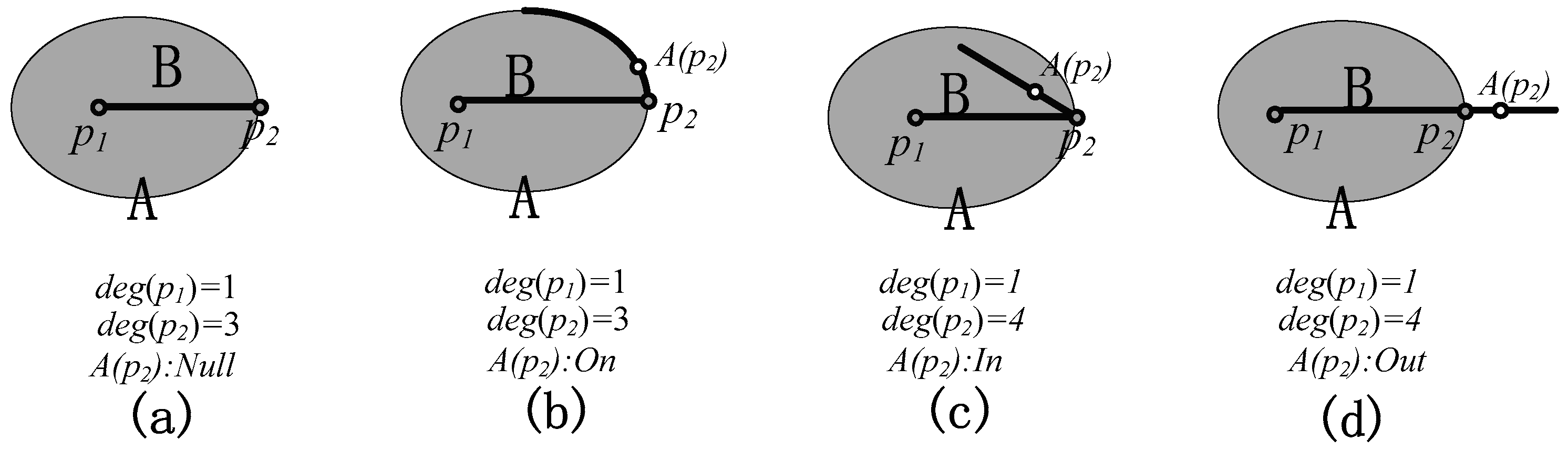
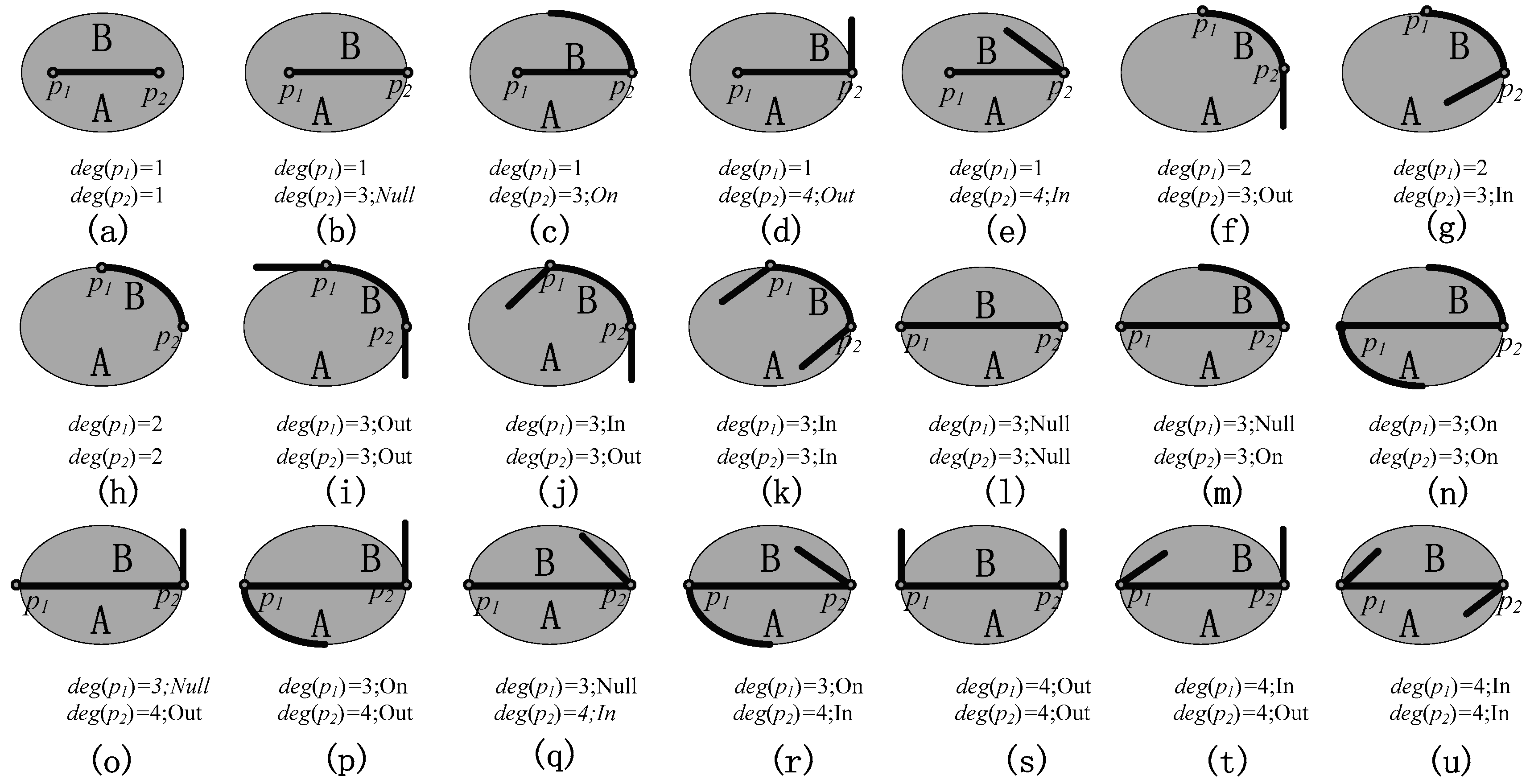
  • Case of degree-pairs (1,1), (1,2), (1,3) and (1,4). If the node degrees of the intersection-line endpoints are both one, the endpoints must be located inside the region and their adjacent point kinds must be Null; otherwise, at least one intersection-line endpoint will be connected with more than one edge. Therefore, there is only one type of degree-pair (1,1), as shown in Figure 9a. If one endpoint is inside the region and the other intersection-line endpoint is not inside, the other endpoint has at least three or more edges connected with it, so there is no degree-pair (1,2). If the node degree of the other endpoint is three, its adjacent point kind must be On (Figure 9b) or Null (Figure 9c), otherwise this endpoint will have 1 adjacent edge or four adjacent edges. Therefore, there are only two types of degree-pair (1,3). If the node degree of the other endpoint is four, its adjacent point kind must be Out (Figure 9d) or In (Figure 9f); otherwise, there will be less than 4 edges meeting at the endpoint.
  • Case of degree-pairs (2,2), (2,3), and (2,4). If the node degrees of the intersection-line endpoints are both two, they must be on the boundary of the region and their adjacent point kinds must be Null; otherwise, the number of edges meeting at the endpoint will not be equal to two. Therefore, there is only one type of degree-pair (2,2), as shown in Figure 9h. If one endpoint is on the boundary of the region and the node degree of the other endpoint is three, its adjacent point kind must be Out (Figure 9f) or In (Figure 9g); otherwise, its endpoint will meet at two edges. Therefore, there are only two types of degree-pair (2,3) and no type of degree-pair (2,4).
  • Case of degree-pairs (3,3) and (3,4). If the node degrees of the intersection-line endpoints are both three, their adjacent point kinds can be Out, In, On, or Null. Therefore, there are six ( C 4 2 ) possible types of degree-pair (3,3), and they are shown in Figure 9i–n, respectively. If the node degree of one endpoint is three and the other is four, the adjacent point kind of the endpoints with node degree 3 must be Null or On, and the adjacent point kind of the endpoints with node degree 4 must be Out or In. Therefore, there are four ( C 2 1 * C 2 1 ) types of degree-pair (3,4), as shown in Figure 9o–r.
  • Case of degree-pairs (4,4). If the node degrees of the intersection-line endpoints are both 4, their adjacent point kinds must be Out or In; otherwise, there will be less than 4 edges meeting at the endpoints. Therefore, there are three asymmetric types of degree-pair (4,4), as shown in Figure 9s–u.
In contrast to the existing methods, our method is complete and can classify more types. For example, the LRBIS method can distinguish only 16 refined types (including two types of intersection-points and one type of disjoint relation). In the LRBIS method, the head-meet and tail-meet relations, HM-cover-by and TM-cover-by relations, and in-cross and out-cross relations are pairwise symmetric, corresponding to the types in Figure 9d,f,j in our method, respectively. The contained-by, EM-cover-by, point-cross, MT-cover-by, on-boundary, belly meet, BM-cover-by, and relation corresponds to the types in Figure 9a,b,d,e,h,i,u, respectively. Therefore, the LRBIS method can only distinguish 10 types of asymmetrical intersection-lines between lines and regions. This method cannot identify the remaining 11 types in Figure 9, such as those shown in Figure 9l,s, and so on. Another matter to note is that the topological intersection component in the LRBIS method is not further subdivided, which makes it insufficient in applications, such as automatic handling of topological conflicts.

3.2. Classification of the Intersection-Line between Line and Line

Compared with lines/regions, there are fewer actual types of intersection-lines between lines. Figure 10 shows the eight types of possible and asymmetric intersection-lines between lines.
Most of the intersection-lines in Figure 10 can be distinguished by the node degrees of the two endpoints of the intersection-lines, except for the (2,2) and (3,3) types. Similarly, the (2,2) type in Figure 10c,d can be distinguished by the kinds of adjacent points, i.e., “Null” and “Out”, as defined in Definition 3.1. However, they cannot be directly used to distinguish the (3,3) type, as shown in Figure 10g,h. Through analysis, although the adjacent point kinds of these two intersection-lines are all Out, the adjacent points are located on the same side of line A in Figure 10g and located on the opposite side of line A in Figure 10h. Therefore, their topological types are different, and the relevant definition is described as follows:
“Definition 3.2” (Same and opposite sides): Let I be an intersection component between lines A and B, points A(p1) and A(p2) be the two adjacent points of L, and c be a circle made with straight-line L(A(p1) A(p2)) as the diameter. Circle c can be divided into two different arcs c1 and c2 by line A. If points A(p1) and A(p2) are on the same arc, then they are on the same side as line A, and the comprehensive type of these two adjacent points is named the same side (SS). If points A(p1) and A(p2) are on different arcs, then they are on the opposite side of line A, and the comprehensive type of these two adjacent points is named the opposite side (OS).
The corresponding proofs of eight types of intersection-line between line and line are as follows. It should be noted that the node degree of their intersection-line endpoints cannot be 4.
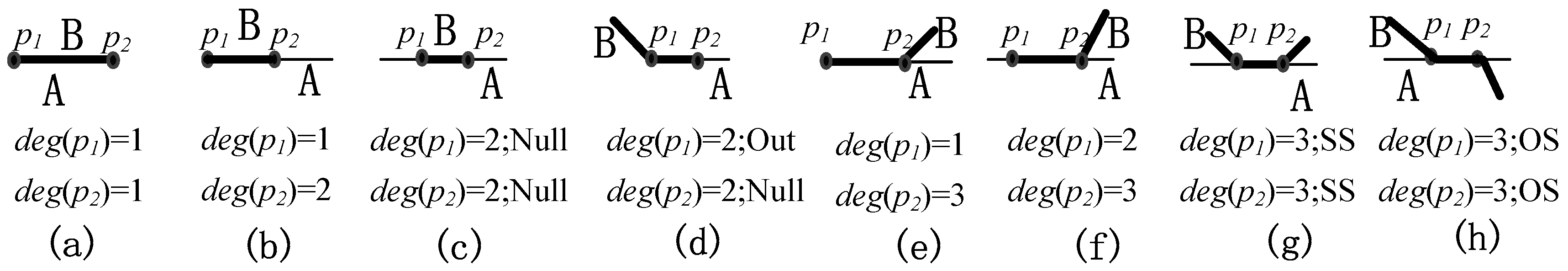
  • Case of degree-pairs (1,1), (1,2), and (1,3). If the node degrees of the intersection-line endpoints are both one, they must be the boundary points of the lines and their adjacent point kinds must be Null (Figure 10a). If one endpoint is on the boundary of a line and the node degree of the other endpoint is two, its adjacent point kind must be Null (Figure 10b). If the node degree of the other endpoint is three, its adjacent point kind must be Out (Figure 10e); otherwise, there will be less than three edges meeting at the endpoint. Therefore, there is only one type of degree-pairs (1,1), (1,2), and (1,3), respectively.
  • Case of degree-pairs (2,2) and (2,3). If the node degrees of the intersection-line endpoints are both two, the adjacent point kind of one endpoint must be Null, and the other one’s adjacent point kind can be Null or Out. Therefore, there are two types of degree-pair (2,2), as shown in Figure 10c,d. If the node degree of one endpoint is three, its adjacent point kind must be Out (Figure 10f); otherwise, there will be less than three edges meeting at the endpoint. Therefore, there is only one type of degree-pair (2,3).
  • Case of degree-pairs (3,3). If the node degree of the intersection-line endpoints is both three, their adjacent point kinds both must be Out, and their comprehensive kinds could be SS or OS. Therefore, there are two asymmetric types of degree-pair (3,3), as shown in Figure 10g,h.
Figure 11a,b show the difference in the comprehensive kinds of adjacent points for the two intersection-lines. This difference can be used to distinguish the two intersection-line node degrees of (3,3), as shown in Figure 10g,h. If the intersection-points between the line and line have two adjacent points, then the comprehensive kinds also apply, as shown in Figure 11c,d.

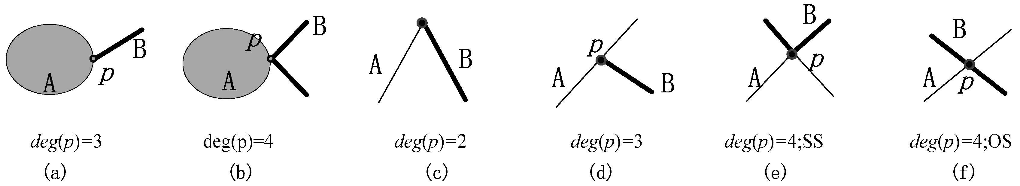
3.3. Classification of the Intersection-Point

Because the node degree of the intersection-point of line/region can be only three or four in R2, there are only two possible types, which can be distinguished by using only node degrees. They are shown in Figure 12a,b. The node degree of the intersection-point of line/line can be two, three, or four in R2. For the node degree of two or three, there is only one possible type of the line/line intersection-point, as shown in Figure 12c,d. For the node degree of four, its possible types of the line/line intersection-point need the comprehensive kinds of adjacent points to distinguish them. As shown in Figure 12e,f, the comprehensive kinds of the two adjacent points of the intersection-point are SS and OS, respectively. Finally, by combining the node degrees and adjacent point kinds, six types of possible and asymmetric intersection-points of line/region and line/line are classified, as shown in Figure 12.

4. Hierarchical Representation of the Topological Relations of Line/Region and Line/Line

Although the refined relations can accurately represent the topological relations between two objects, they require more topological details to be described and calculated, so they are usually used in fields like topological conflict detection and processing [1]. However, fields like spatial data organization and query only need coarse relations. Therefore, to meet different application requirements, it is necessary to study the hierarchical representation of topological relations between spatial objects [1,2,16,20]. In this paper, referring to the strategy in Reference [2], the E-WID model is used to represent the coarse line/region (and line/line) relations, while the N-WWIS model is used to represent the refined line/region (and line/line) relations.

4.1. Using the E-WID Model to Represent Coarse Relations

The description framework of the E-WID mode is shown in Equation (2). Where the value of fDi denotes the content and dimension, fE denotes the Euler number, the set operations intersection (∩), and the difference (\) are based on whole objects A and B, and their spatial components are topologically complete. The value of fDi can be one element of {−1, 0, 1, 2, 3, 4, 5, 6} in 2D space.
R ( A , B ) = [ f D i ( A B ) f E ( A B ) f D i ( A \ B ) f D i ( B \ A ) f E ( A \ B ) f E ( B \ A ) ]
The E-WID model can describe the topological relations between any two spatial objects in 2D space, so it can also be used to distinguish the coarse topological relations of line/region and line/line. For line/region and line/line, there are only five cases (value of fDi) of the intersection or difference components, i.e., empty (−1), pure zero-dimensional point (0), pure one-dimensional line (1), pure 2D region (2) and a mixture of point and line (3). The value of fE can be any natural number, and its expression is ignored when the spatial component is empty.
For the line/region relations, although the E-WID model is coarse, it can discriminate an infinite number of coarse relations because a line and a region can have an infinite number of intersection components (or difference components), and the value of fE can reflect the differences between them. In this paper, only the relations with a single intersection (or disjoint relation) that can be distinguished by the E-WID model are illustrated, as shown in Figure 13. Among them, Figure 13a is disjoint, and Figure 13b,c both have only one zero-dimensional intersection, but one is inside of line B and the other is on the boundary of line B; Figure 13d–j all have only one one-dimensional intersection. The topological configurations in Figure 13d–j are as follows: Line B is contained by region A (Figure 13d), B is covered by A but only one endpoint is on the boundary of A (Figure 13e), B overlaps with A but has no endpoint on the boundary of A (Figure 13f), the one-dimensional intersection is on the boundary of A (Figure 13g), B is covered by A and its endpoints are both on the boundary of A (Figure 13h), B overlaps with A and has one endpoint on the boundary of A (Figure 13i), and B crosses A (Figure 13j). It is worth noting that some elements of the matrix in Figure 13 are ignored when they are empty (there are no corresponding spatial components), and this expression follows that of Zhou et al. (2013). The specific reason is that it can show the difference between them and elements whose intersection is not empty but whose Euler number is zero.
Similarly, the E-WID model can also discriminate an infinite number of line/line coarse relations. Figure 14 shows the line/line coarse relations with a single intersection distinguished by the E-WID model. Among them, Figure 14a is disjoint, Figure 14b–d all have only one 0-dimensional intersection, and Figure 13e–j all have only one one-dimensional intersection.

4.2. Using the N-WWIS Model to Represent Refined Relations

As mentioned earlier, the coarse relations do not directly describe the dimensions and topological types of each intersection component. However, in some applications, such as conflict detection and processing, we need to deal with each intersection component according to the topological type; therefore, it is necessary to represent and calculate the relations with multiple intersection components at a refined level. Since Section 3 fully classified the intersection component types of line/region and line/line based on the node degree (and adjacent point kinds), the N-WWIS model is effectively established and can be used to represent the refined line/region and line/line relations.
Figure 15 shows two line/region relations with multiple intersection components. Although they both contain four intersection-lines and one intersection-point in Figure 5a,b, the dimension, sequence, and topological types of each component are not all the same. These two refined relations with different topological configurations are indistinguishable by the coarse model (E-WID), and the refined model (N-WWIS) must be used. The result of the N-WWIS description in Figure 15 reflects the difference between them. For example, the description result of the intersection component with sequence 2 is 2 (1, <4Out, 3On>) in Figure 15a. Where the number outside the bracket indicates its sequence number (i.e., two), the first number in the bracket indicates the dimension (i.e., 1-dimensional), and the expression <4Out, 3On> in the rest bracket indicates its topological type, which corresponds to the symmetrical type in Figure 9p. The description result of the intersection component with sequence 2 is 2 (1, 4Out, 4In) in Figure 15b, where the dimension is 1 (intersection-line) and the topological type is <4Out, 4In> (i.e., the symmetrical type in Figure 9t).
Figure 16 also shows two different line/line relations that cannot be distinguished by the E-WID model but can be distinguished by the N-WWIS model. These two models both have two intersection-lines and two intersection-points, but the types of intersection components with the same sequence are different, and the N-WWIS model can fully describe and differentiate them. For example, the intersection component with sequence number 2 is an intersection-line in Figure 16a, and its topological type is <4SS, 4SS>, i.e., the node degrees of the two endpoints are both four, and their adjacent points are on the same side of line A. In Figure 16a, the intersection component with sequence number 2 is an intersection-point, its topological type is <4SS>, i.e., its node degree is four, and the adjacent points are also on the same side of line A.

5. Experimental Application

To evaluate our refined model (N-WWIS) and its application, a prototype system based on the N-WWIS model is developed in Microsoft Visual C# 2010 environment along with Oracle database. Its user interface is shown in Figure 17.
The prototype system was intensively tested using the OpenStreetMap (OSM) data of Changsha city, Hunan Province, China, as experimental data (July 2019, as shown in Figure 17). The area of the test region is 1938 km2, including 8688 traffic lines and 277 water regions, which correspond to the TRAFFIC LINE layer and WATER-AREA layer in Figure 17, respectively. Since the number of real conflicts in OSM data is unknown, 19 additional traffic lines, which have conflicting relations with water-area, are simulated to evaluate the N-WWIS model. In addition, to highlight the results of topological conflict detection, we place the relevant intersection components on the temporary work layers. For example, the intersection-lines and intersection-points between the traffic line and water region are placed in the TWINSECTLINE layer and the TWINSECTPOINT layer, respectively.
In these experiments, the traffic line is used as an example of the line, and the water region is used as an example of the region. An object-oriented (or object-relational) spatiotemporal data model [2,32] and a rule-based model transformation method [33,34] are adopted for data transformation. In addition, to deal with potential topological conflicts, a set of rules (336 for line/regions and 165 lines/lines) is developed based mainly on the N-WWIS refined relations and the attributes of spatial objects.
Taking lines/regions as an example, the strategies for topological checking and dealing are described as follows:
  • Download OSM data (XML format), and convert them to the Chinese national fundamental geographic information data model using the transformation method and the object-oriented spatiotemporal data model.
  • Set the tolerance (i.e., 1 m) based on experience for the computation of refined lines/regions topological relations.
  • Select one line Li (1 ≤ in) from the line data set and use the Minimal Bounding Rectangle of Li as the regions to filter out the data. This can reduce the number of regions that have no intersection with the line Li.
  • Calculate the refined N-WWIS topological relations between the line Li and the filtered regions automatically, and store the non-disjoint regions and the refined descriptions of their relations to form the intersection components (include intersection-line and intersection-point) types set {A, B,…, W}.
  • Return to Steps 3 and 4, start the calculation of refined relations between another line and the filtered regions and store relevant data until all objects in the line data set have been calculated.
  • For each intersection component in the types set, match it to the rules set for automatically (or semi-automatically) dealing with each potential topological conflict.
The topological conflict detection results of the test data and example explanations will be expanded below.

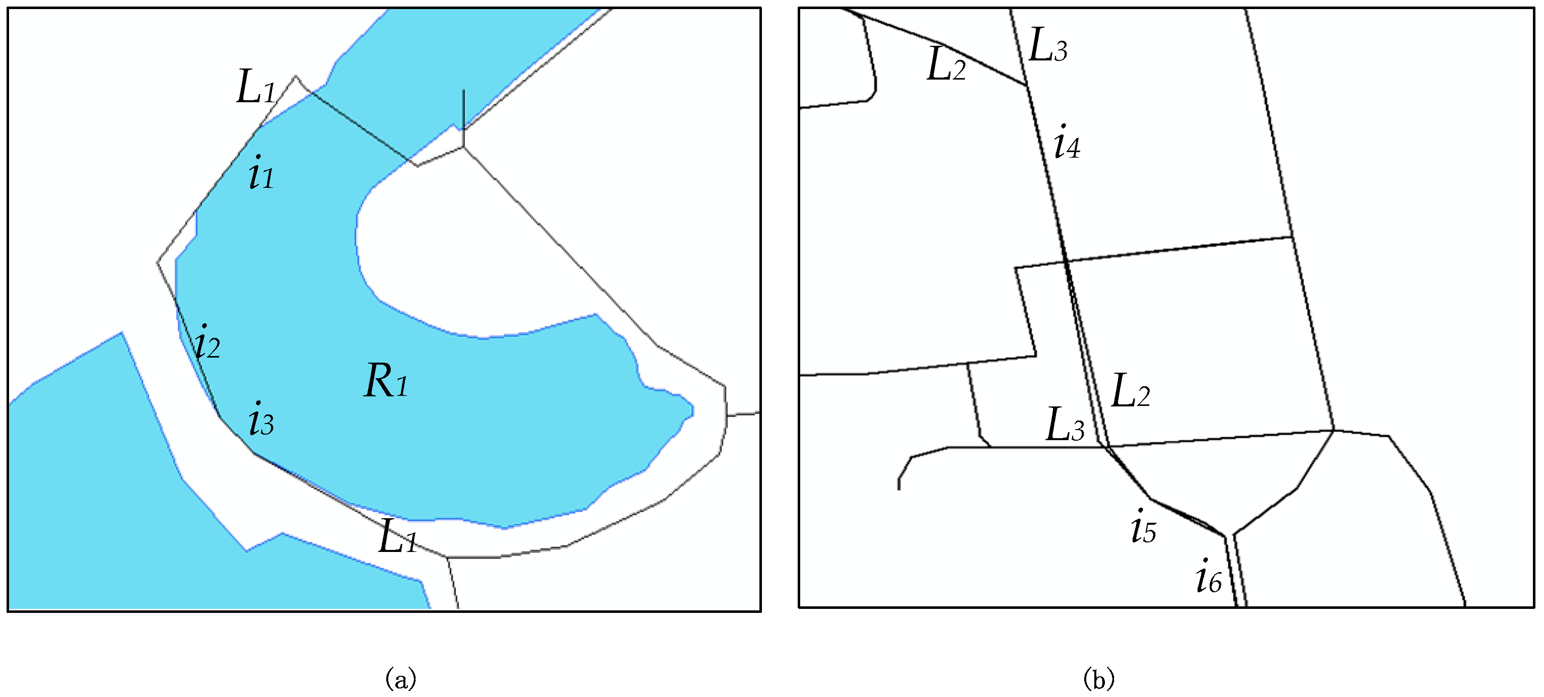
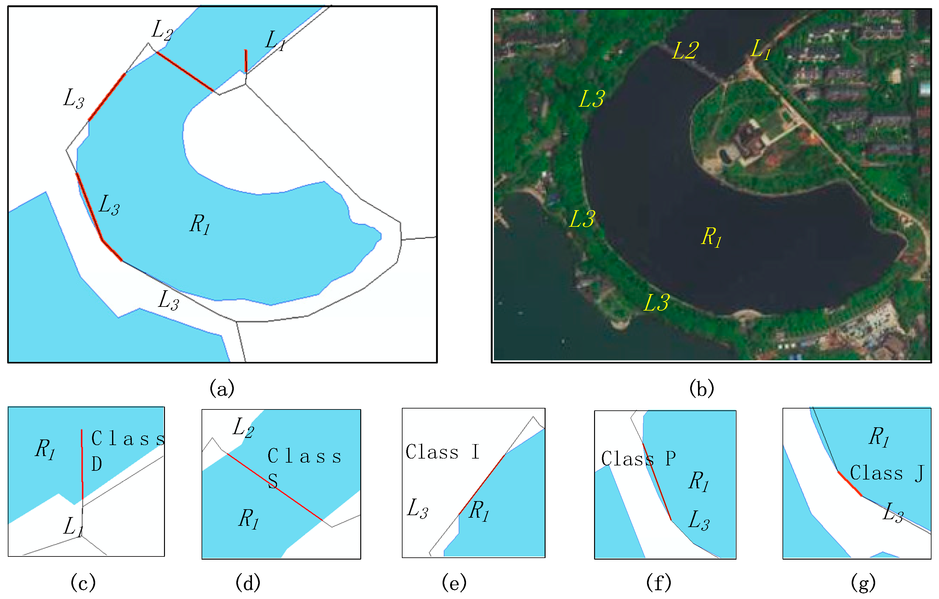
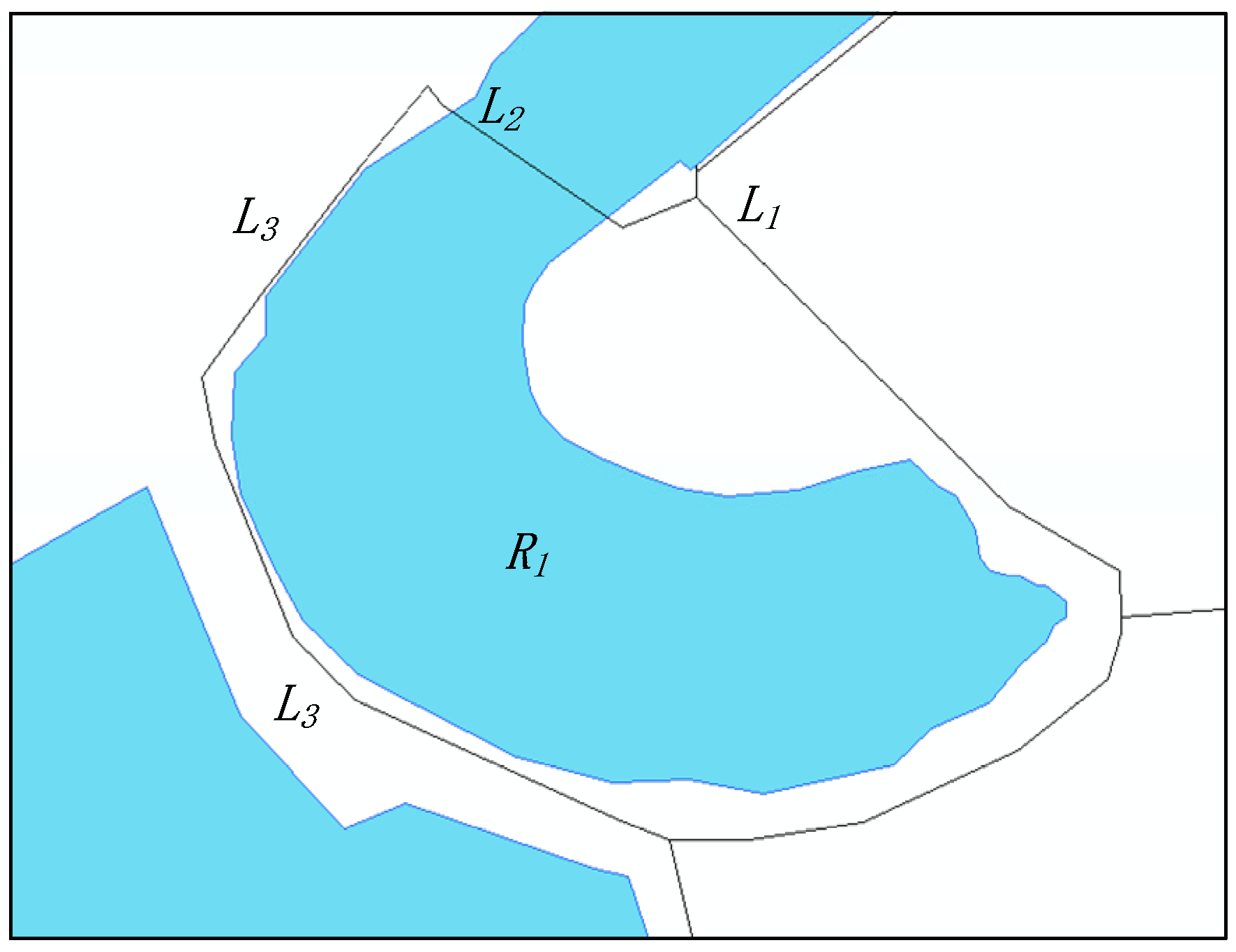
5.1. Examples of Intersection Components between Lines and Regions

After detecting the topological conflicts between traffic lines and water regions in the test data, a total of 221 intersection components were found, including 210 intersection-lines and 11 intersection-points. For easy identification, the intersection-line types in Figure 9 and the intersection-point types in Figure 12 are named as class A (corresponding to Figure 9a), class B (Figure 9b), class C (Figure 9c), …, class V (Figure 12a), and class W (Figure 12b) in our system. Table 1 shows the detection results of the intersection components types between traffic lines and water regions. The number of each type of intersection components in the experimental results is shown in the third and sixth columns of Table 1. The classes H, K, M, N, Q, R, and U shown in red number are generated from simulated data. It can be seen that all the intersection components types between traffic lines and water regions can be detected by our model.
According to the attribute table of the INSECTLINE layer and INSECTPOINT layer, the types of each intersection component and the traffic and water region object involved can be queried. Figure 18a shows a partial amplification drawing of the test region, where water region R1 has multiple intersecting-lines with traffic lines (L1, L2, and L3), and Figure 18b shows the satellite image of the corresponding area. The class (type) of intersection-line between region R1 and line L1 is D (Figure 18c), which corresponds to type <1, 4Out> in Figure 9d; The class of intersection-line between region R1 and line L2 is S (Figure 18d), and its type corresponds to <4Out, 4Out> in Figure 9s. The classes of intersection-lines between region R1 and line L3 is I (Figure 18e), P (Figure 18f), and J (Figure 18g), and their corresponding types are <3Out, 3Out> (Figure 9k), <3On, 4Out> (Figure 9p), and <3In, 3Out > (Figure 9j), respectively.
Referring to the actual situation (satellite images), the potential topological conflicts of lines/regions in Figure 18 are addressed as follows: in Figure 18c, the part (intersection-line) of the traffic line L1 that falls into the water region R1 needs to be cut out; in Figure 18b, the involved data do not need to be modified because the intersection-line is usually a bridge; in Figure 18d, the position of line L3 at the intersection needs to move to a certain position away from region R1; in Figure 18e, the part of line L3 at the intersection-line may need to be modified to keep it from falling into the lake; finally, in Figure 18f, the direction of line L3 at the intersection-line needs to be adjusted so that it is not tangent to region R1. Similarly, other types of topological conflict dealing rules are established in our system based on the topological types of intersection components and the actual situation. According to the rule set we established, the corresponding conflict addressing results in Figure 18a are shown in Figure 19.

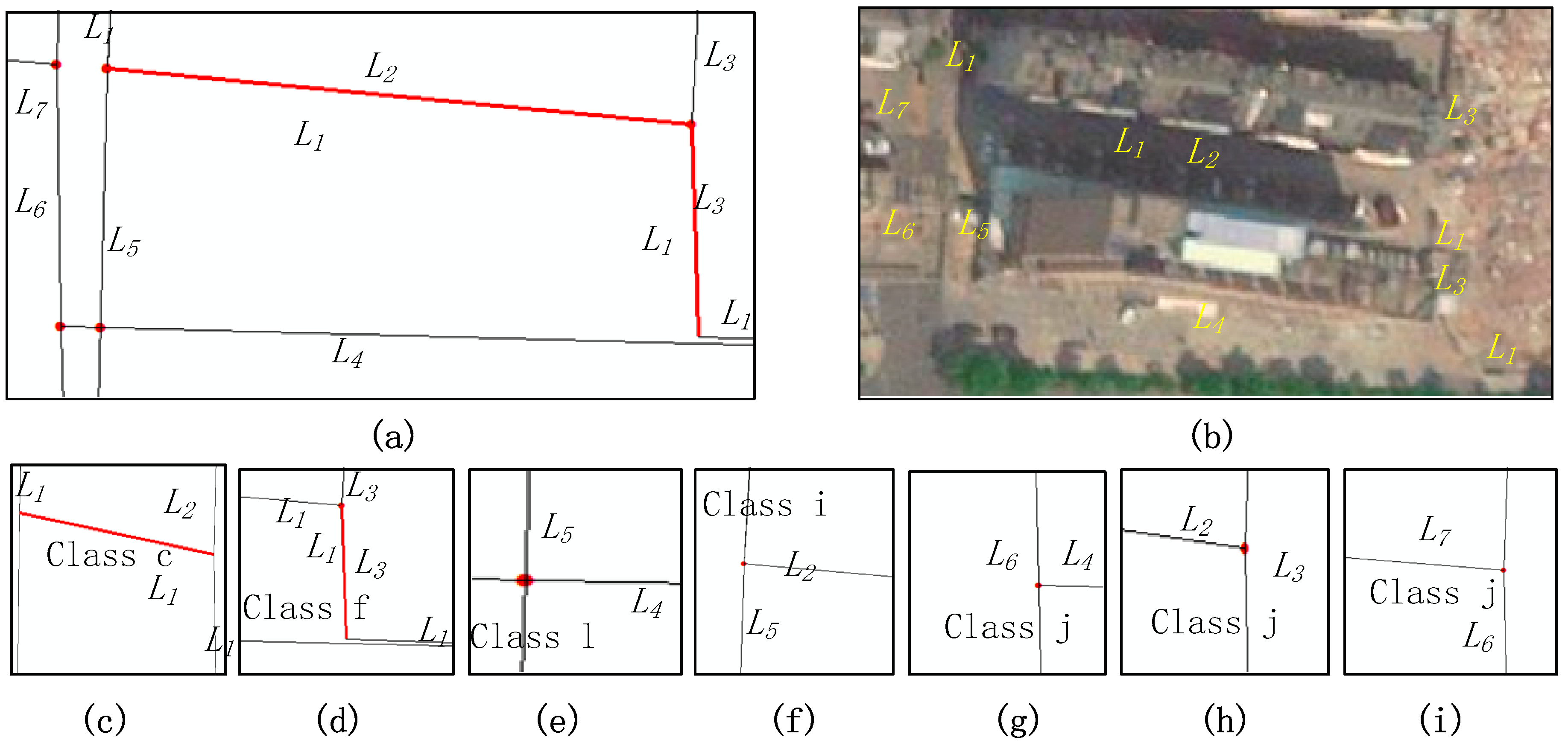
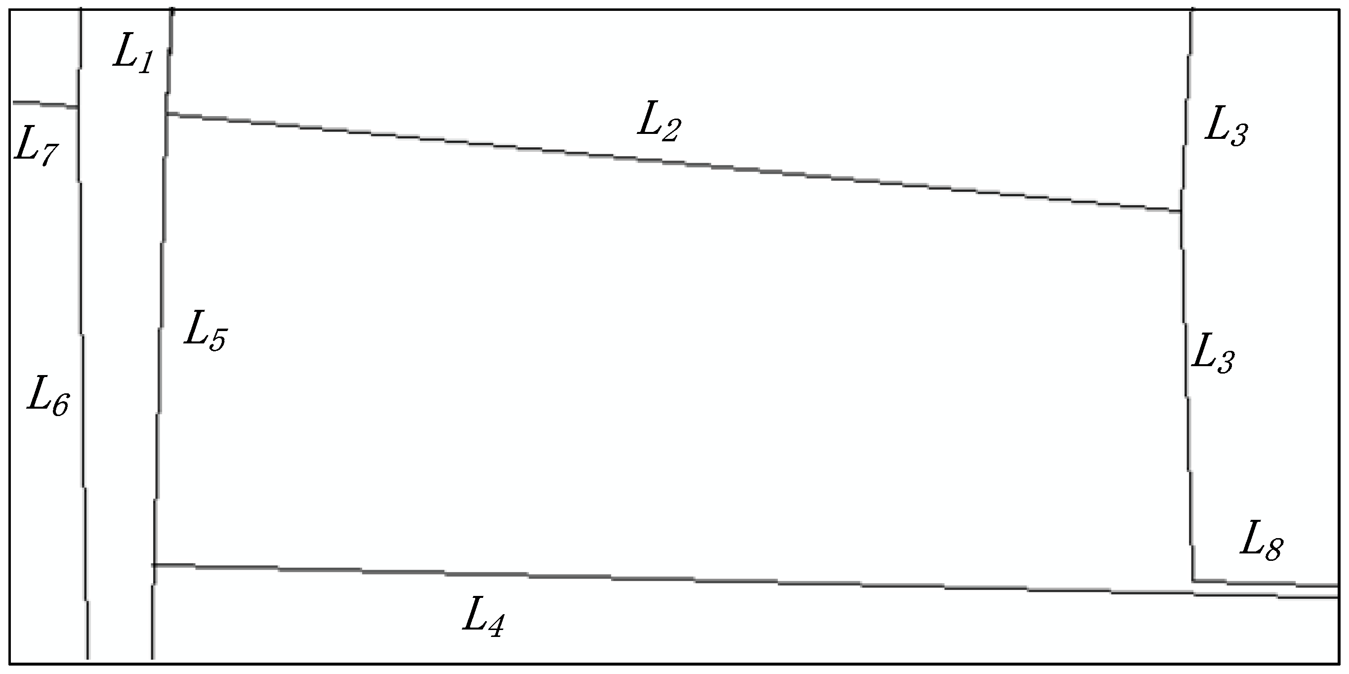
5.2. Examples of Intersection Components between Lines

In our system, the intersection-line types in Figure 10a–h are named as class a to class h, and the intersection-point types between lines/lines in Figure 12c–f are named as class i to class l. By calculating the intersection components of traffic lines in the test data, 22 intersection-lines and 9694 intersection-points are obtained, and these components are placed in temporary layers TTINSECTLINE and TTINSECTPOINT, respectively. Table 2 shows the detection results of the intersection components types between traffic lines. The specific numbers of the corresponding classes are shown in Table 2. It can be seen that the intersection components between traffic lines are mainly intersection-points, but there are also some intersection-lines with different types (classes).
Figure 20a shows the line/line intersection component of the local area in the test data, and Figure 20b shows the satellite image of the corresponding area. Among them, there are one intersection-line of class c (Figure 20c), one intersection-line of class f (Figure 20d), one intersection-point of class l (Figure 20e), one intersection-point of class i (Figure 20f), and three intersection-points of class j (Figure 20g–i).
In the ordinary case, when there is an intersection-line between two traffic lines, only one traffic line is reserved in the intersection part unless they are up and down. For intersecting-lines of class c (<2Null, 2Null>), it is usual to delete the covered line. However, the actual situation (satellite images) is sometimes complicated. For example, the line L2 covered by L1 in Figure 20c should be retained, while the overlapped parts of the intersecting line L2 should be removed. The case of class f (<2, 3>) is similar; usually, the overlapping part of L3 should be deleted, but according to the actual situation, the overlapping part of L1 should be deleted (Figure 20d). For intersecting-points of class l (<4OS>), the two traffic lines of communication should be interrupted at the intersection unless they are up and down too, and the broken lines should be deleted if they are very short (Figure 20e). For intersecting-points of class i (<2>), they usually do not need to change (Figure 20f) or merge the two lines; For intersecting-points of class j (<3>), they usually do not need to change (Figure 20g–i) or one of the two lines need be interrupted at the intersection-point. According to the rule set and some manual assistance, the corresponding conflict dealing results in Figure 20a are shown in Figure 21.

6. Conclusions and Discussion

In this paper, we present a refined line/region and line/line topological relation model (N-WWIS). This model is a complement and development of the E-WID and E-WWIS hierarchical models for regions/regions. To conform to cognitive habit, the spatial objects are defined based on manifold topology rather than point set topology, and the intersection components are defined based on whole-whole (rather than decomposed) object intersection sets in this model. The topological invariant of node degree is introduced to distinguish the topological type of the intersection component between line/region and line/line. By combining node degree and adjacent point kinds (“Null”, “On”, “In”, “Out”, “SS”, and “OS”), 29 types of possible and asymmetric intersection-lines are distinguished, including 21 types of lines/regions and 8 types of lines/lines). By using this method, we also find two types of lines/regions and four types of line/line intersection-points. Therefore, a hierarchical topological relationship model has been formed for line/region and line/line, i.e., the E-WID model is used at the coarse level and the N-WWIS model is used at the refined level.
The corresponding algorithms for calculating the intersection component type of line/region and line/line are implemented, and application examples in automatic topological integrity checking are provided. The developed system was intensively tested using the OSM data of Changsha city, Hunan Province, China, as experimental data. The results of this study represent a new avenue for checking and handling automatic topological integrity.
The topological relations between regions/points, lines/points, and points/points can be completely discriminated by the E-WID model (Figure 22). Therefore, the topological relations between two simple objects in 2D space can be represented and discriminated by E-WID at a coarse level, and E-WWIS and BBIS (if necessary) are used for region/region, and N-WWIS is used for line/region and line/line at a refined level hierarchically.
As mentioned by the reference [35], applications of three-dimensional (3D) GIS have increased in scope and complexity, which in turn are driving an increasing demand for the creation and maintenance of reliable 3D GIS. However, the existing 3D data sets contain many topological inconsistencies [36], which restrict the sustainable development of related applications. On the other hand, manifold topology theory, the operand (i.e., the whole object), the set operations (i.e., intersection and difference), the topological invariants (i.e., content, dimension, Euler number, and degree of point), and some adjacent point kinds (“Null”, “On”, “In”, and “Out”) used in our hierarchical models can also be used in 3D space in theory. Therefore, the expansion of our models (including E-WID and E/N-WWIS) to 3D spatial objects based on manifold topology will be our future work.

Author Contributions

Conceptualization, Xiaoguang Zhou; methodology, Xiaoguang Zhou. and Hongyuan He; formal analysis, Dongyang Hou; writing—original draft, Hongyuan He and Dongyang Hou; validation, Hongyuan He, Rui Li and Heng Zheng; Writing—review & editing, Hongyuan He and Dongyang Hou. All authors have read and agreed to the published version of the manuscript.

Funding

This research was funded by the National Natural Science Foundation of China (Project No. 41971360).

Institutional Review Board Statement

The study did not require ethical approval.

Informed Consent Statement

Not applicable.

Data Availability Statement

The data presented in this study are available on request from the corresponding author.

Acknowledgments

The authors would like to thank the anonymous reviewers for their constructive and valuable comments that significantly contributed to improving this paper.

Conflicts of Interest

The authors declare no conflict of interest.

References

  1. Egenhofer, M.; Franzosa, R. Point-set Topological Spatial Relations. Int. J. Geogr. Inf. Sci. 1991, 5, 161–174. [Google Scholar] [CrossRef] [Green Version]
  2. Egenhofer, M.; Herring, J. Categorizing Binary Topological Relationships between Regions, Lines, Points in Geographic Databases. In A Framework for the Definitions of Topological Relationships and An Algebraic Approach to Spatial Reasoning within This Framework; NCGIA Technical Reports; National Center for Geographic Information and Analysis: Santa Barbara, CA, USA, 1991; pp. 91–97. [Google Scholar]
  3. Egenhofer, M.; Sharma, J.; Mark, D. A Critical Comparison of the 4-Intersection and 9-Intersection Models for Spatial Relations: Formal Analysis. In Autocarto 11; McMaster, R., Armstrong, M., Eds.; American Society for Photogrammetry and Remote Sensing: Bethesda, MD, USA, 1993. [Google Scholar]
  4. Clementini, E.; Felice, P.D. A Comparison of Methods for Representing Topological relationships. Inf. Sci. 1995, 3, 149–178. [Google Scholar] [CrossRef]
  5. Chen, J.; Li, C.M.; Li, Z.L.; Christopher, G. A Voronoi-based 9-intersection model for spatial relations. Int. J. Geogr. Inf. Sci. 2001, 15, 201–220. [Google Scholar] [CrossRef]
  6. Shen, J.; Zhou, T.; Chen, M. A 27-Intersection Model for Representing Detailed Topological Relations between Spatial Objects in Two-Dimensional Space. ISPRS Int. Geo-Inf. 2017, 6, 37. [Google Scholar] [CrossRef] [Green Version]
  7. Egenhofer, M.; Mark, D.M. Modeling Conceptual Neighborhoods of Topological Line-Region Relations. Int. J. Geogr. Inf. Sci. 1995, 9, 555–565. [Google Scholar] [CrossRef]
  8. Kurara, Y.; Egenhofer, M. The 9+ intersection for topological relationships between a directed line segment and a region. In Workshop on Behavior and Monitoring Interpretation; Gottfried, B., Ed.; CEUR-WS.org: Munich, Germany, 2007; pp. 62–76. [Google Scholar]
  9. Formica, A.; Mazzei, M.; Pourabbas, E.; Rafanelli, M. Enriching the semantics of the directed polyline–polygon topological relationships: The DLP-intersection matrix. J. Geogr. Syst. 2017, 192, 13–19. [Google Scholar] [CrossRef]
  10. Shen, J.; Huang, Y.; Chen, M. Topological relations between a directed line and a directed region. Trans. GIS 2020, 24, 526–548. [Google Scholar] [CrossRef]
  11. Deng, M.; Cheng, T.; Chen, X.; Li, Z. Multi-level Topological Relations between Spatial Regions Based Upon Topological Invariants. Geoinformatica 2007, 11, 239–267. [Google Scholar] [CrossRef]
  12. Randell, D.; Cui, Z.; Cohn, A. A spatial logical based on regions and connection. In Proceedings of the 3rd International Conference on Knowledge Representation and Reasoning, Cambridge, MA, USA, 25–29 October 1992; Kaufmann, M., San, M., Eds.; Springer: Berlin/Heidelberg, Germany; New York, NY, USA, 1992; pp. 165–176. [Google Scholar]
  13. Cui, Z.; Cohn, A.; Randell, D. Qualitative and Topological Relationships in Spatial Databases. In Proceedings of the Third International Symposium on Advances in Spatial Databases, Singapore, 23–25 June 1993; Abel, D., Ooi, B.C., Eds.; Springer: Singapore, 1993; pp. 293–315. [Google Scholar]
  14. Li, Z.L.; Zhao, R.; Chen, J. A Voronoi-based spatial algebra for spatial relations. Prog. Nat. Sci. 2002, 12, 50–58. [Google Scholar]
  15. Zhou, X.G.; Chen, J.; Zhan, F.B.; Li, Z.; Madden, M.; Zhao, R.L.; Liu, W.Z. A Euler-number-based Topological Computation Model for Land Parcel Database Updating. Int. J. Geogr. Inf. Sci. 2013, 27, 1983–2005. [Google Scholar] [CrossRef]
  16. Deng, M. A Hierarchical Representation of Line-Region Topological Relations. Int. Arch. Photogramm. Remote Sens. Spatial Inf. Sci. 2008, XXXVII, 25–30. [Google Scholar]
  17. Clementini, E.; Di, F.P. Topological invariants for lines. IEEE Trans. Knowl. Data. Eng. 1998, 10, 38–54. [Google Scholar] [CrossRef]
  18. Wu, C. Detailed model of topological and metric relationships between a line and region. Arab. J. Geosci. 2019, 12, 130. [Google Scholar] [CrossRef]
  19. Li, Z.L.; Deng, M. A hierarchical approach to the line-line topological relations. In Progress in Spatial Data Handling; Springer: Heidelberg, Germany, 2006; pp. 365–382. [Google Scholar]
  20. Egenhofer, M.; Franzosa, R. On the Equivalence of Topological Relations. Int. J. Geogr. Inf. Sci. 1995, 9, 133–152. [Google Scholar] [CrossRef]
  21. Li, Z.L.; Li, Y.L.; Chen, Y.Q. Basic Topological Models for Spatial Entities in 3-dimensional Space. GeoInformatica 2000, 4, 419–433. [Google Scholar] [CrossRef]
  22. Liu, K.; Shi, W. Extended model of topological relationships between spatial objects in geographic information systems. Int. J. Appl. Earth Obs. Geoinf. 2007, 9, 264–275. [Google Scholar] [CrossRef]
  23. ISO. 19107. In Geographic Information–Spatial Schema; Technical Report; ISO: Geneva, Switzerland, 2003.
  24. Lee, J.M. Introduction to Topological Manifolds; Springer: New York, NY, USA, 2011. [Google Scholar]
  25. Tu, L.W. An Introduction to Manifolds, 2nd ed.; Springer: New York, NY, USA, 2011. [Google Scholar]
  26. Muscat, J.; Buhagiar, D. Connective Spaces. Mem. Fac. Sci. Eng. Shimane Univ. 2006, 39, 1–13. [Google Scholar]
  27. Clementini, E.; Felice, P.D. A model for representing topological relationships between complex geometric features in spatial databases. Inf. Sci. 1996, 90, 121–136. [Google Scholar] [CrossRef]
  28. Schneider, M.; Behr, T. Topological relationships between complex spatial objects. ACM Trans. Database Sys. 2006, 31, 39–81. [Google Scholar] [CrossRef]
  29. Armstrong, M.A. Basic Topology; McGraw-Hill Book Company: London, UK, 1979. [Google Scholar]
  30. Euler, L. Solutio problematis ad geometriam situs pertinentis. Comment. Acad. Sci. Petropolitanae 1741, 8, 128–140. [Google Scholar]
  31. Frank, H. Graph Theory; Addison-Wesley: Reading, MA, USA, 1969. [Google Scholar]
  32. Bondy, J.A.; Murty, U.S.R. Graph Theory; Springer: Berlin, Germany, 2008; Volume 311, pp. 359–372. [Google Scholar]
  33. Zhao, Y.J.; Zhou, X.G.; Li, G.Q.; Xing, H.F. A Spatio-Temporal VGI Model Considering Trust-Related Information. ISPRS Int. Geo-Inf. 2016, 5, 10. [Google Scholar] [CrossRef] [Green Version]
  34. Zhou, X.G.; Zeng, L.; Jiang, Y.; Zhou, K.; Zhao, Y. Dynamic Integrating OSM data to Borderland Database. ISPRS Int. Geo-Inf. 2015, 4, 1707–1728. [Google Scholar] [CrossRef] [Green Version]
  35. Girindran, R.; Boyd, D.; Rosser, J.; Vijayan, D.; Long, G.; Robinson, D. On the Reliable Generation of 3D City Models from Open Data. Urban Sci. 2020, 4, 47. [Google Scholar] [CrossRef]
  36. Giovanella, A.; Bradley, P.E.; Wursthorn, S. Evaluation of Topological Consistency in CityGML. ISPRS Int. J. Geo-Inf. 2019, 8, 278. [Google Scholar] [CrossRef] [Green Version]
Figure 1. Examples of multiple intersection components between line/region and line/line in OpenStreetMap (OSM) data. (a) A lake has multiple intersection components with the same trajectory; (b) One trajectory multiple intersection components with another trajectory.
Ijgi 10 00015 g001
Figure 2. The incompleteness of the LRBIS (intersections set between line and region boundary) method. (a) A in-cross type defined by the LRBIS method; (b) A out-cross type defined the LRBIS method; (c) A point-cross type defined the LRBIS method; (d) One cross type omitted by the LRBIS method; (e) The other cross type omitted by the LRBIS method.
Ijgi 10 00015 g002
Figure 3. Spatial objects in 2D space and their boundary points and interior points based on manifold topology. (a) Simple region (2-manifold) in R2, its interior point has a neighbourhood homeomorphic to R2, its boundary point has a neighbourhood homeomorphic to H2; (b) Simple line (1-manifold) in R2, its interior point has a neighbourhood homeomorphic to R1, its boundary point has a neighbourhood homeomorphic to H1; (c) Simple line (0-manifold) in R2, its interior point has a neighbourhood homeomorphic to R0, it has no boundary point.
Ijgi 10 00015 g003
Figure 4. Example of differences between topological intersection components and spatial intersection components. (a) Region A and line B; (b) Topological components of A∩B; (c) Spatial components of A∩B.
Ijgi 10 00015 g004
Figure 5. Examples of 1-dimensional intersection relations of line/region and line/line that cannot be distinguished by “Euler number”, i.e., fE(A\IL) and fE(B\IL), but can be distinguished by “degree of point”. (a) Region A intersects line B with a intersection-line on the boundary; (b) Region A intersects line B with a intersection-line inside region A; (c) One case that line A intersects line B with a intersection-line; (d) The other case Line A intersects line B with a intersection-line.
Ijgi 10 00015 g005
Figure 6. Examples of the degree of a certain point in the union of two spatial objects. (a) A point with degree value one in the union of two lines; (b) A point with degree value two in the union of two lines; (c) A point with degree value three in the union of two lines; (d) A point with degree value four in the union of two lines; (e) A point with degree value one in the union of a line and the boundary of a region; (f) A point with degree value two in the union of a line and the boundary of a region; (g) A point with degree value three in the union of a line and the boundary of a region; (h) A point with degree value four in the union of a line and the boundary of a region.
Ijgi 10 00015 g006
Figure 7. Intersection-line types of line/region that can be distinguished by node degree. (a) Case of degree-pair (1,1); (b) Case of degree-pair (1,3); (c) Case of degree-pair (1,4); (d) Case of degree-pair (2,2); (e) Case of degree-pair (2,3); (f) Case of degree-pair (3,3); (g) Case of degree-pair (3,4); (h) Case of degree-pair (4,4).
Ijgi 10 00015 g007
Figure 8. Examples of the intersection-lines that cannot be distinguished by only node degree but can be distinguished by the combination of node degree and adjacent point kinds. (a) Case of degree-pair (1,3) and the adjacent point kind of p2 is Null; (b) Case of degree-pair (1,3) and the adjacent point kind of p2 is On; (c) Case of degree-pair (1,4) and the adjacent point kind of p2 is In; (d) Case of degree-pair (1,4) and the adjacent point kind of p2 is Out.
Ijgi 10 00015 g008
Figure 9. Twenty-one types of possible and asymmetric intersection-lines between lines and regions. (a) Case of degree-pair (1,1); (b) Case of degree-pair (1,3) and the adjacent point kind of p2 is Null; (c) Case of degree-pair (1,3) and the adjacent point kind of p2 is On; (d) Case of degree-pair (1,4) and the adjacent point kind of p2 is Out; (e) Case of degree-pair (1,4) and the adjacent point kind of p2 is In; (f) Case of degree-pair (2,3) and the adjacent point kind of p2 is Out; (g) Case of degree-pair (2,3) and the adjacent point kind of p2 is In; (h) Case of degree-pair (2,2); (i) Case of degree-pair (3,3) and the adjacent point kinds of p1 and p2 are both Out; (j) Case of degree-pair (3,3) and the adjacent point kinds of p1 is In and p2 is Out; (k) Case of degree-pair (3,3), and the adjacent point kinds of p1 and p2 are both In; (l) Case of degree-pair (3,3), and the adjacent point kinds of p1 and p2 are both Null; (m) Case of degree-pair (3,3), and the adjacent point kinds of p1 is Null and p2 is On; (n) Case of degree-pair (3,3), and the adjacent point kinds of p1 and p2 are both On; (o) Case of degree-pair (3,4), and the adjacent point kinds of p1 is Null and p2 is Out; (p) Case of degree-pair (3,4), and the adjacent point kinds of p1 is On and p2 is Out; (q) Case of degree-pair (3,4), and the adjacent point kinds of p1 is Null and p2 is In; (r) Case of degree-pair (3,4), and the adjacent point kinds of p1 is On and p2 is In; (s) Case of degree-pair (4,4), and the adjacent point kinds of p1 and p2 are both Out; (t) Case of degree-pair (4,4), and the adjacent point kinds of p1 is In and p2 is Out; (u) Case of degree-pair (4,4), and the adjacent point kinds of p1 and p2 are both In.
Ijgi 10 00015 g009
Figure 10. Eight types of possible and asymmetric intersection-lines between lines. (a) Case of degree-pair (1,1); (b) Case of degree-pair (1,2); (c) Case of degree-pair (2,2) with Null adjacent point kind; (d) Case of degree-pair (2,2) with Null and Out adjacent point kind; (e) Case of degree-pair (1,3); (f) Case of degree-pair (2,3); (g) Case of degree-pair (3,3) with SS comprehensive adjacent point kind; (h) Case of degree-pair (3,3) with OS comprehensive adjacent point kind.
Ijgi 10 00015 g010
Figure 11. Comprehensive kinds of adjacent points of the intersection components between lines. (a) The comprehensive adjacent point kinds of intersection-line are same side; (b) The comprehensive adjacent point kinds of intersection-line are opposite side; (c) The comprehensive adjacent point kinds of intersection-point are same side; (d) The comprehensive adjacent point kinds of intersection- point are opposite side.
Ijgi 10 00015 g011
Figure 12. Six types of possible and asymmetric intersection-points of line/region and line/line. (a) The degree value of intersection-point between line/region is three; (b) The degree value of intersection-point between line/region is four; (c) The degree value of intersection-point between lines is two; (d) The degree value of intersection-point between lines is three; (e) The degree value of intersection-point between lines is four, and its comprehensive adjacent point kind is SS; (f) The degree value of intersection-point between lines is four, and its comprehensive adjacent point kind is OS.4. Hierarchical Representation of the Topological Relations of Line/Region and Line/Line.
Ijgi 10 00015 g012
Figure 13. The line/region coarse relations with a single intersection distinguished by the Euler number-based whole object intersection and difference (E-WID) model. (a) Region A and line B are disjoint; (b) The zero-dimensional intersection is inside of line B; (c) The zero-dimensional intersection is on the boundary of line B; (d) Line B is contained by region A; (e) Line B is covered by region A, but only one endpoint is on the boundary of A; (f) Line B overlaps with region A, but there is no endpoint on the boundary of A; (g) The one-dimensional intersection is on the boundary of region A; (h) Line B is covered by region A and its endpoints are both on the boundary of A; (i) Line B overlaps with region A and has one endpoint on the boundary of A; (j) Line B crosses region A.
Ijgi 10 00015 g013
Figure 14. The line/line coarse relations with a single intersection distinguished by the E-WID model. (a) Line A and B are disjoint; (b) The zero-dimensional intersection is on the boundary of both line A and B; (c) The zero-dimensional intersection is inside of line B and on the boundary of line B; (d) The zero-dimensional intersection is inside of both line A and B; (e) The one-dimensional intersection contains one endpoint of line A and one endpoint of line B; (f) Line B is contained in line A; (g) The one-dimensional intersection is inside of both line A and B; (h) Line B is covered by line A; (i) Line A is equal to line B; (j) The one-dimensional intersection is inside of line A and contains one endpoint of line B.
Ijgi 10 00015 g014
Figure 15. Two examples of relations between line and region that cannot be distinguished by the E-WID model but can be distinguished by the node degree-based whole-whole object intersection sets (N-WWIS) model. (a) One case that the intersection components between region A and line B are four intersection-lines and one intersection-point; (b) The other case that the intersection components between region A and line B are four intersection-lines and one intersection-point.
Ijgi 10 00015 g015
Figure 16. The refined relations between two lines in two examples that cannot be distinguished by the E-WID model but can be distinguished by the N-WWIS model. (a) One case that the intersection components between line A and line B are two intersection-lines and two intersection-point; (b) The other case that the intersection components between line A and line B are two intersection-lines and two intersection-point.
Ijgi 10 00015 g016
Figure 17. The user interface of the prototype system and experimental data.
Ijgi 10 00015 g017
Figure 18. Examples of the intersection component types between traffic lines and water regions in the test data. (a) Intersection components between traffic lines and water regions; (b) Satellite images of the corresponding area; (c) The class (type) of intersection-line is D; (d) The class of intersection-line is S; (e) The class of intersection-line is I; (f) The class of intersection-line is P; (g) The class of intersection-line is J.
Ijgi 10 00015 g018
Figure 19. Examples of topological conflict addressing results between lines/regions.
Ijgi 10 00015 g019
Figure 20. Examples of the intersection component types between traffic lines in the test data. (a) Intersection components between traffic lines; (b) Satellite images of the corresponding area; (c) The class(type) of intersection-line is h; (d) The class of intersection-point is l; (e) The class of intersection-point is j; (f) The class of intersection-point is l; (gi) The class of intersection-point is l.
Ijgi 10 00015 g020
Figure 21. Examples of topological conflict dealing results between lines.
Ijgi 10 00015 g021
Figure 22. Topological relations between points/regions, points/lines, and points/points, as discriminated by the E-WID model. (a) Region A and point B are disjoint; (b) Point B is on the boundary of region A; (c) Point B is inside of region A; (d) Line A and point B are disjoint; (e) Point B is on the boundary of line A; (f) Point B is inside of line A; (g) Point A and point B are disjoint; (h) Point A is equal to point B.
Ijgi 10 00015 g022
Table 1. Detection results of the intersection components types between traffic lines and water regions.
ClassTypeNumberClassTypeNumber
A<1, 1>
(Figure 9a)
5M<3Null, 3On>
(Figure 9m)
1
B<1, 3Null>
(Figure 9b)
3N<3On, 3On>
(Figure 9n)
1
C<1, 3On>
(Figure 9c)
15O<3Null, 3Out>
(Figure 9o)
7
D<1, 4Out>
(Figure 9d)
17P<3On, 3Out>
(Figure 9p)
2
E<1, 4In>
(Figure 9e)
9Q<3Null, 4In>
(Figure 9q)
1
F<2, 3Out>
(Figure 9f)
2R<3On, 4In>
(Figure 9r)
1
G<2, 3In>
(Figure 9g)
8S<4Out, 4Out>
(Figure 9s)
121
H<2, 2>
(Figure 9h)
1T<4In, 4Out>
(Figure 9t)
7
I<3Out, 3Out>
(Figure 9i)
3U<4In, 4In>
(Figure 9u)
1
J<3In, 3Out>
(Figure 9j)
1V<3>
(Figure 12a)
7
K<3In, 3In>
(Figure 9k)
1W<4>
(Figure 12b)
4
L<3Null, 3Null>
(Figure 9l)
3
Table 2. Detection result of the topological conflict between traffic lines.
ClassCorresponding TypeNumber
a<1, 1> (Figure 10a)2
b<1, 2> (Figure 10b)1
c<2Null, 2Null> (Figure 10c)4
d<2Out, 2Null> (Figure 10d)1
e<1, 3> (Figure 10e)1
f<2, 3> (Figure 10f)6
g<3SS, 3SS> (Figure 10g)4
h<3OS, 3OS> (Figure 10h)3
i<2> (Figure 12c)3793
j<3> (Figure 12d)4162
k<4SS> (Figure 12e)25
l<4OS> (Figure 12f)1714
Publisher’s Note: MDPI stays neutral with regard to jurisdictional claims in published maps and institutional affiliations.

