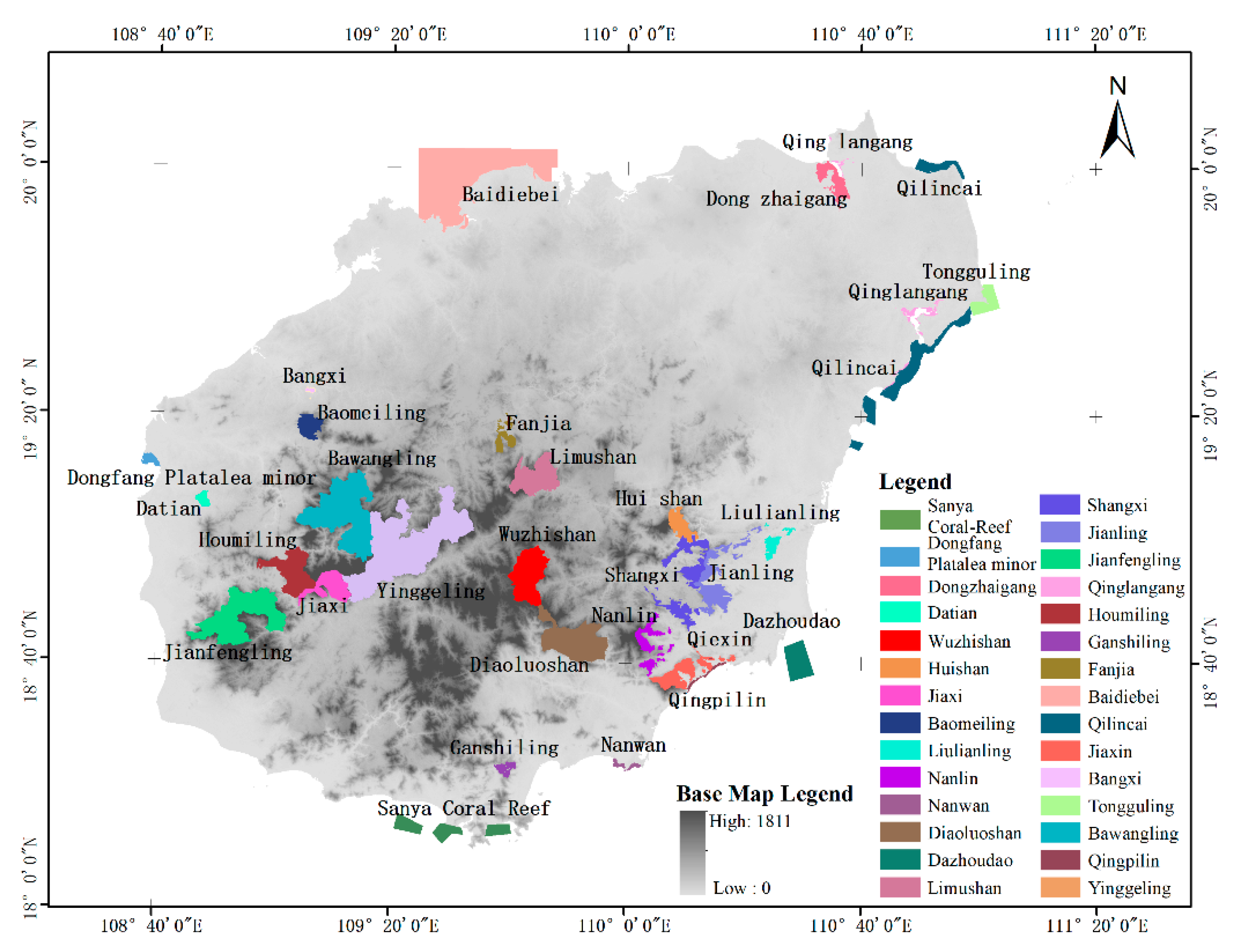
Figure 1.
Distribution of 29 provincial and national nature reserves at Hainan Island.
Figure 1.
Distribution of 29 provincial and national nature reserves at Hainan Island.
Figure 2.
Examples for datasets A and B. (a1,a2) True color images. (a3,a4) False color composites of the near-infrared, green, and blue bands (NIR, G, B). (b1–b4) Corresponding labels.
Figure 2.
Examples for datasets A and B. (a1,a2) True color images. (a3,a4) False color composites of the near-infrared, green, and blue bands (NIR, G, B). (b1–b4) Corresponding labels.
Figure 3.
Examples in the public dataset. (a1–a4) True color images. (b1–b4) Corresponding labels.
Figure 3.
Examples in the public dataset. (a1–a4) True color images. (b1–b4) Corresponding labels.
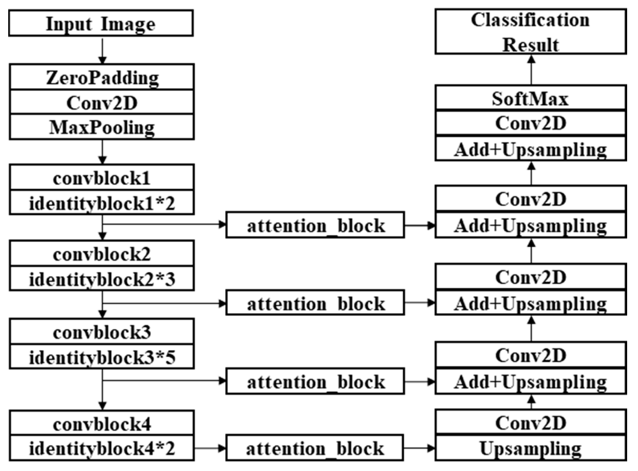
Figure 4.
Structure of ResMANet (residual multi-attention network).
Figure 4.
Structure of ResMANet (residual multi-attention network).
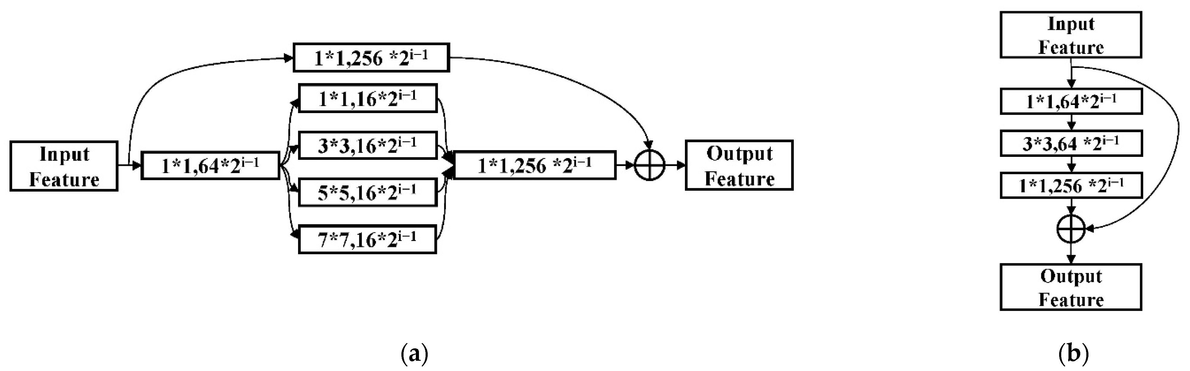
Figure 5.
Structures of the modules in the encoder. (a) Conv_block. (b) Identity_block. i: The convolution stage.
Figure 5.
Structures of the modules in the encoder. (a) Conv_block. (b) Identity_block. i: The convolution stage.
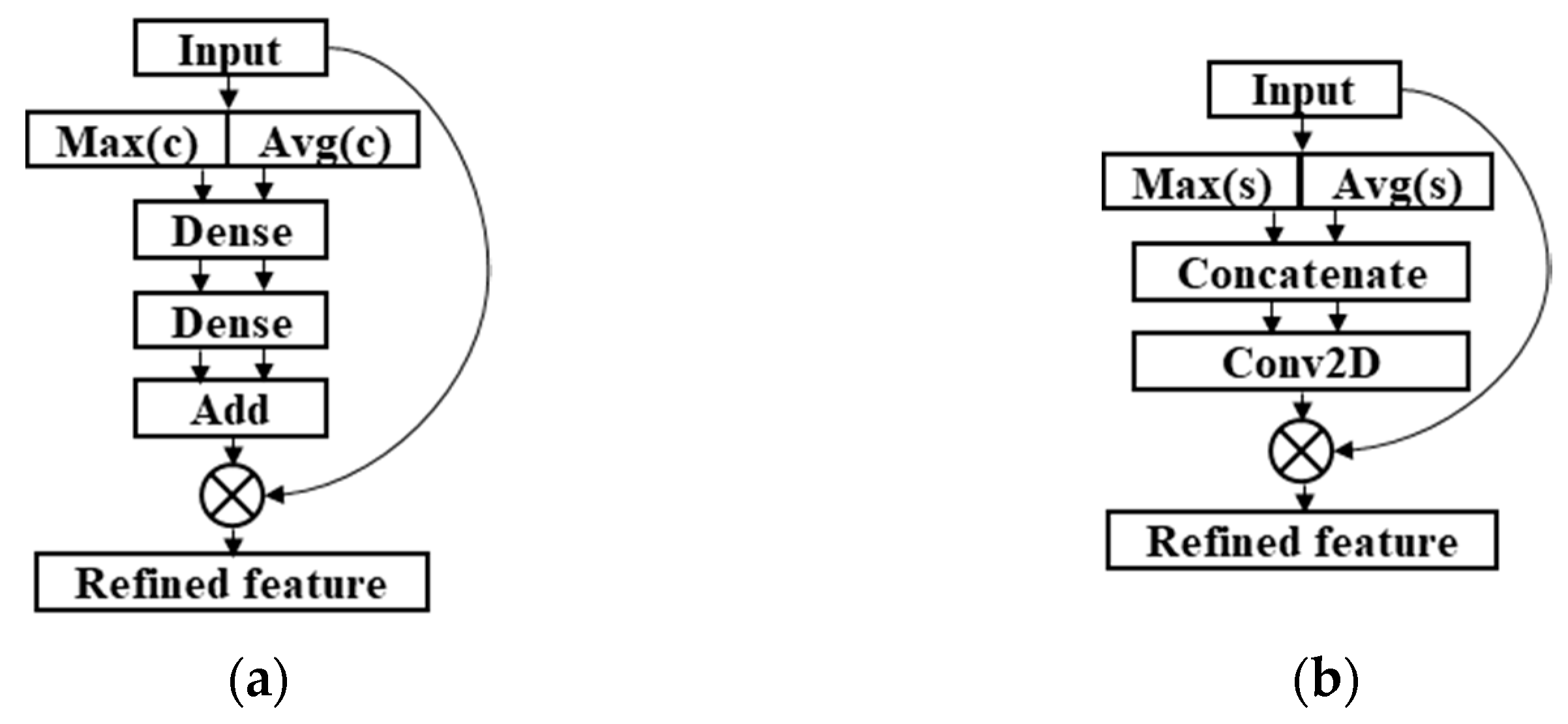
Figure 6.
Structures of the attention modules. (a) Channel attention module. (b) Spatial attention module.
Figure 6.
Structures of the attention modules. (a) Channel attention module. (b) Spatial attention module.
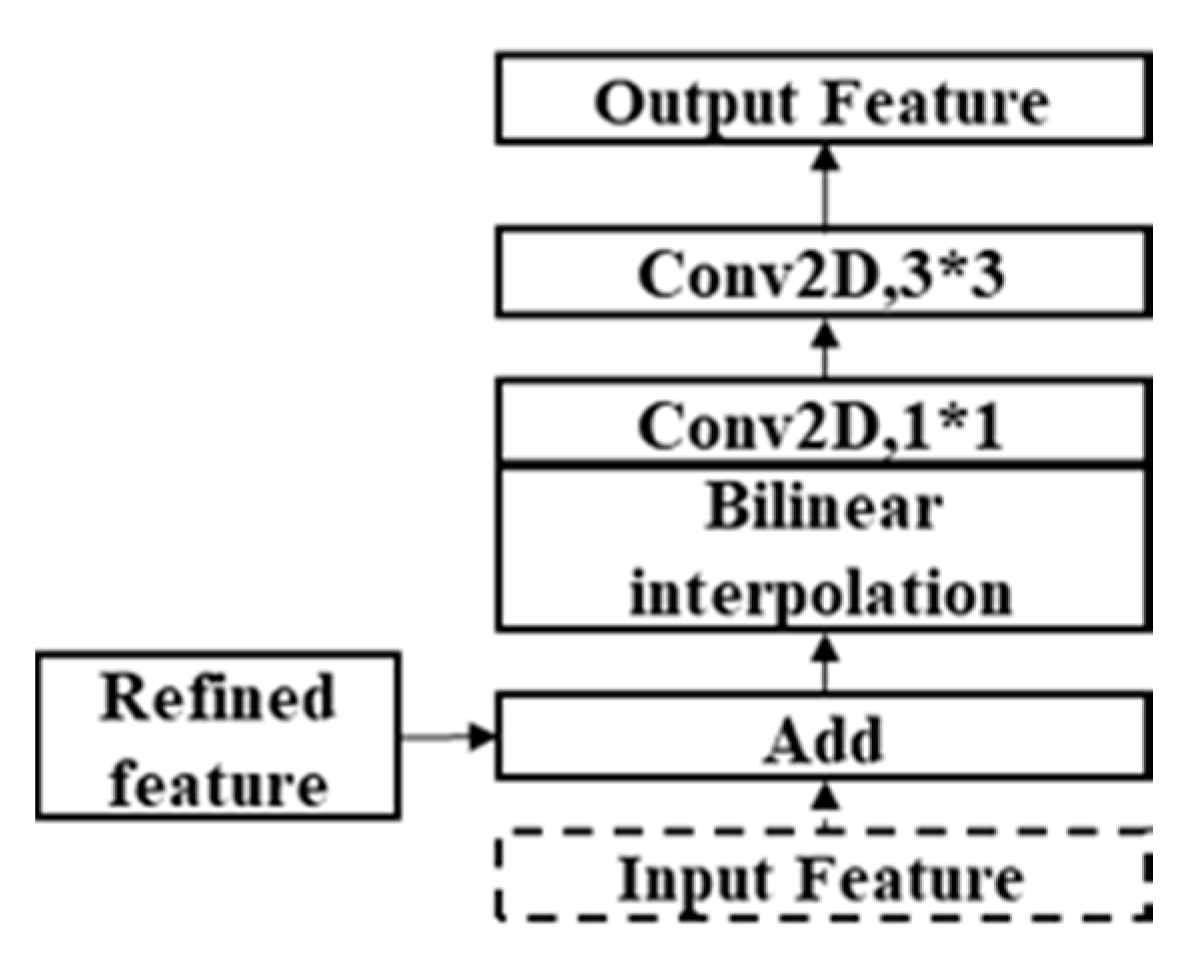
Figure 7.
Upsampling module.
Figure 7.
Upsampling module.
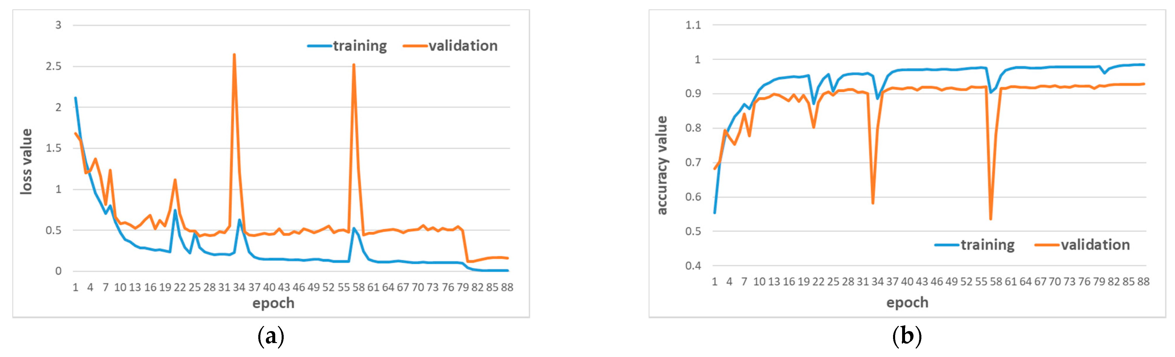
Figure 8.
Training process for Hainan dataset A. (a) Loss curve. (b) Accuracy curve
Figure 8.
Training process for Hainan dataset A. (a) Loss curve. (b) Accuracy curve
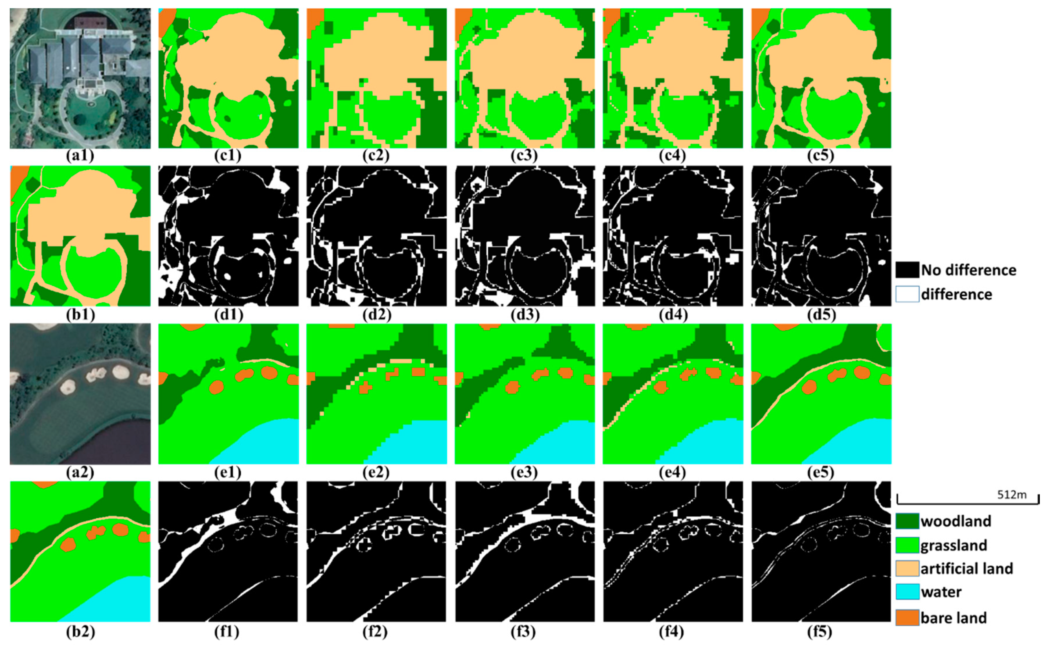
Figure 9.
Prediction examples in the validation set of dataset A. (a1,a2) True color images. (b1,b2) Ground truth images. (c1–c5,e1–e5) Predictions of U-Net, PSPNet (ResNet-50), DeepLabv3+ (ResNet-50), U-Net (ResNet-50) and ResMANet. (d1–d5,f1–f5) Corresponding difference maps.
Figure 9.
Prediction examples in the validation set of dataset A. (a1,a2) True color images. (b1,b2) Ground truth images. (c1–c5,e1–e5) Predictions of U-Net, PSPNet (ResNet-50), DeepLabv3+ (ResNet-50), U-Net (ResNet-50) and ResMANet. (d1–d5,f1–f5) Corresponding difference maps.
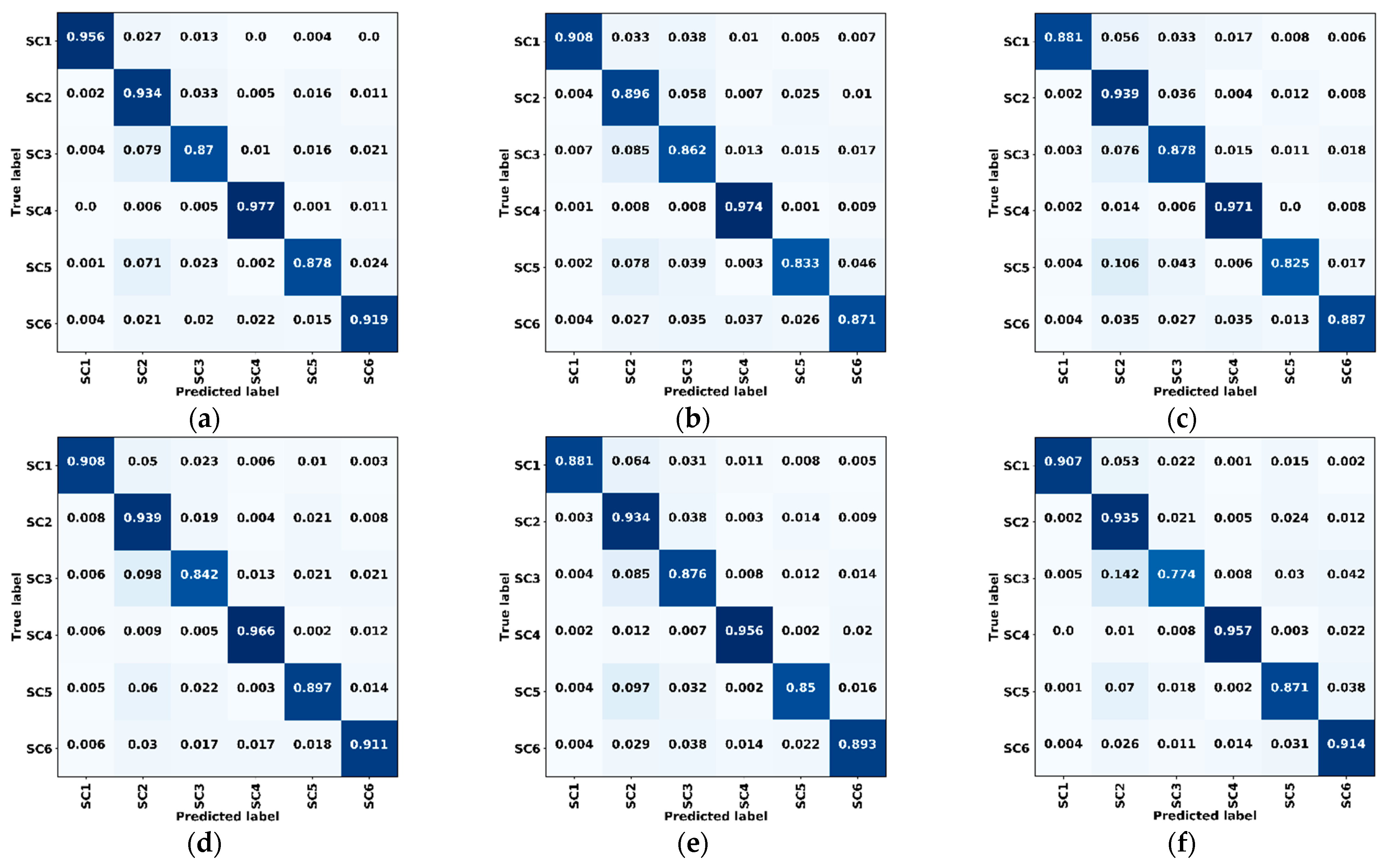
Figure 10.
Confusion matrices of validation data for dataset A. (a) ResMANet. (b) U-Net. (c) PSPNet (ResNet-50). (d) DeepLabv3+ (ResNet-50). (e) U-Net (ResNet-50). (f) ResMANet (CEL). SC1: Farmland, SC2: Woodland, SC3: Grassland, SC4: Water, SC5: Artificial land, SC6: Bare land, CEL: Cross-entropy loss.
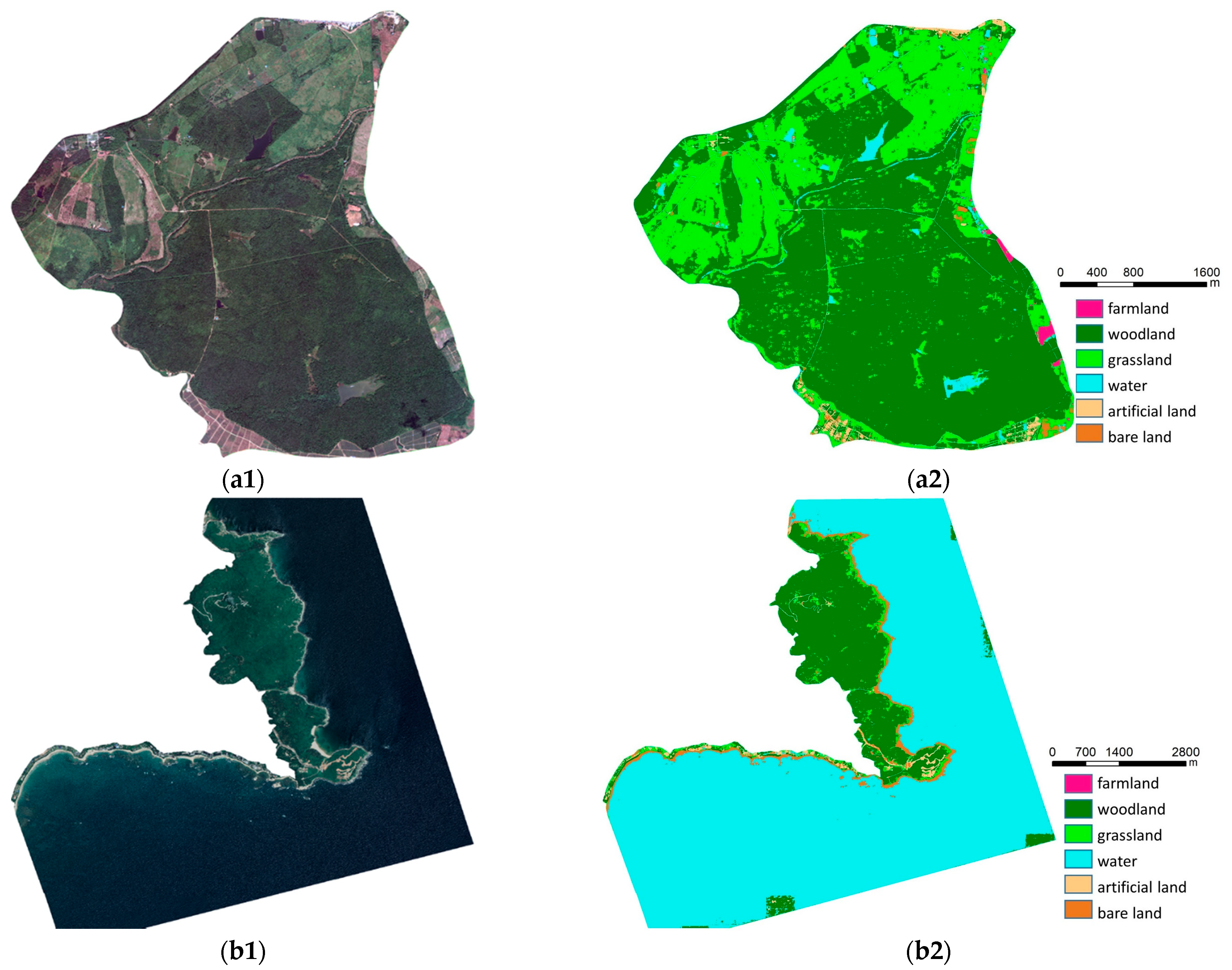
Figure 11.
Classification results for nature reserves based on true color images. (a1) Image of Datian Nature Reserve. (a2) Label of Datian Nature Reserve. (b1) Image of Tongguling Nature Reserve. (b2) Label of Tongguling Nature Reserve.
Figure 11.
Classification results for nature reserves based on true color images. (a1) Image of Datian Nature Reserve. (a2) Label of Datian Nature Reserve. (b1) Image of Tongguling Nature Reserve. (b2) Label of Tongguling Nature Reserve.
Figure 12.
Training process for Hainan dataset B. (a) Loss curve. (b) Accuracy curve.
Figure 12.
Training process for Hainan dataset B. (a) Loss curve. (b) Accuracy curve.
Figure 13.
Prediction examples in the validation set of dataset B. (a1,a2) False color images composited by the NIR, G, and B bands. (b1,b2) Ground truth images. (c1–c5,e1–e5) Predictions of U-Net, PSPNet (ResNet-50), DeepLabv3+ (ResNet-50), U-Net (ResNet-50) and ResMANet. (d1–d5,f1–f5) Corresponding difference maps.
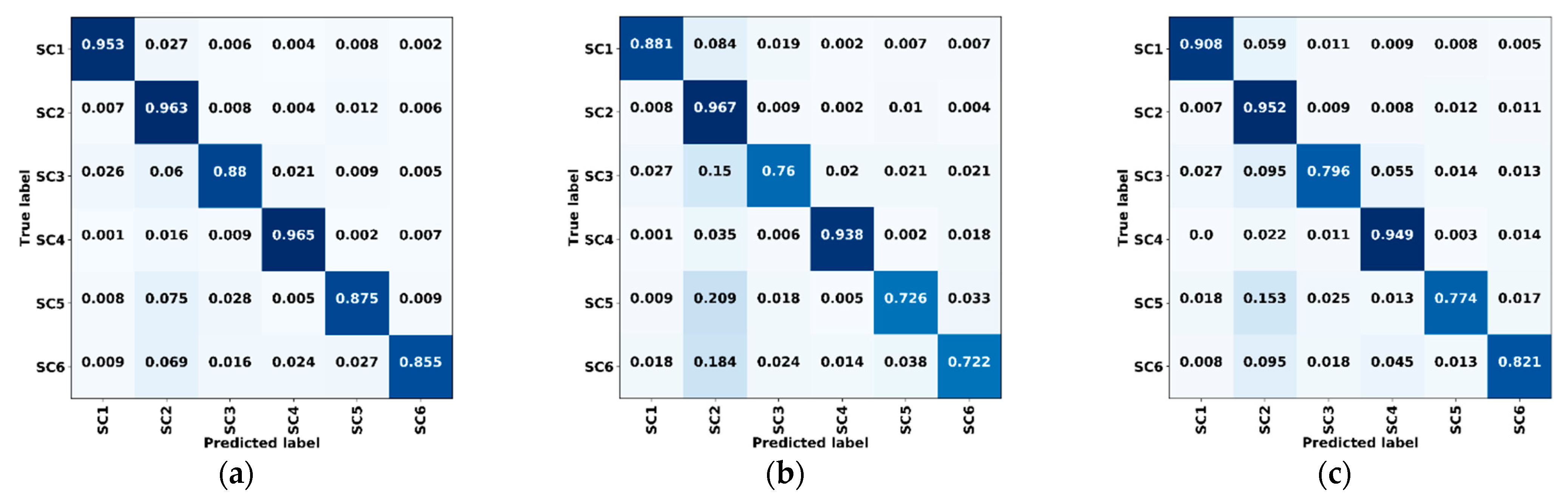
Figure 14.
Confusion matrices of validation data in Dataset B. (a) ResMANet. (b) U-Net. (c) PSPNet (ResNet-50). (d) DeepLabv3+ (ResNet-50). (e) U-Net (ResNet-50). (f) ResMANet (CEL). SC1: Farmland, SC2: Woodland, SC3: Grassland, SC4: Water, SC5: Artificial land, SC6: Bare land, CEL: Cross-entropy loss.
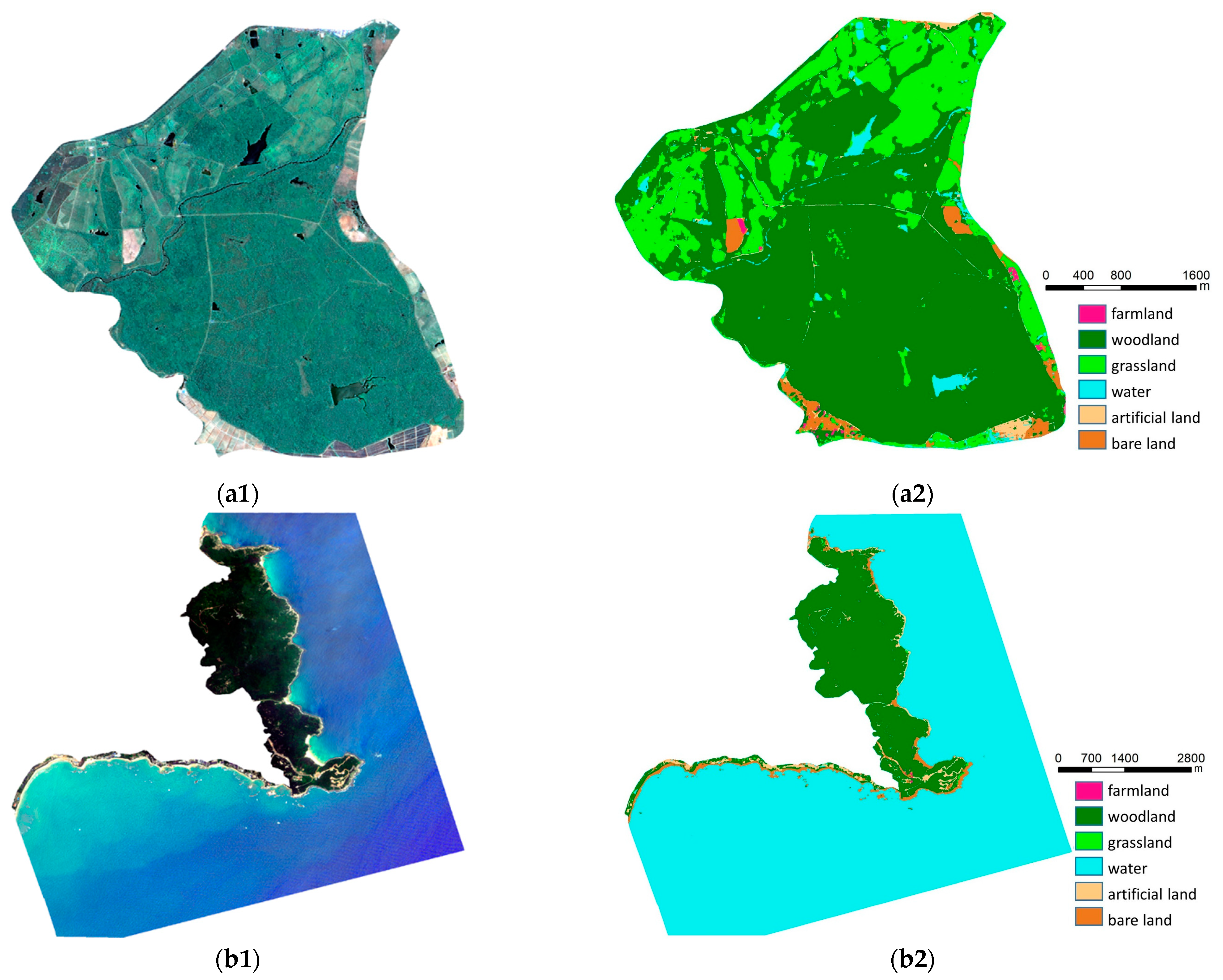
Figure 15.
Classification results for nature reserves based on multi-spectral images. (a1) Image of Datian Nature Reserve. (a2) Label of Datian Nature Reserve. (b1) Image of Tongguling Nature Reserve. (b2) Label of Tongguling Nature Reserve.
Figure 15.
Classification results for nature reserves based on multi-spectral images. (a1) Image of Datian Nature Reserve. (a2) Label of Datian Nature Reserve. (b1) Image of Tongguling Nature Reserve. (b2) Label of Tongguling Nature Reserve.
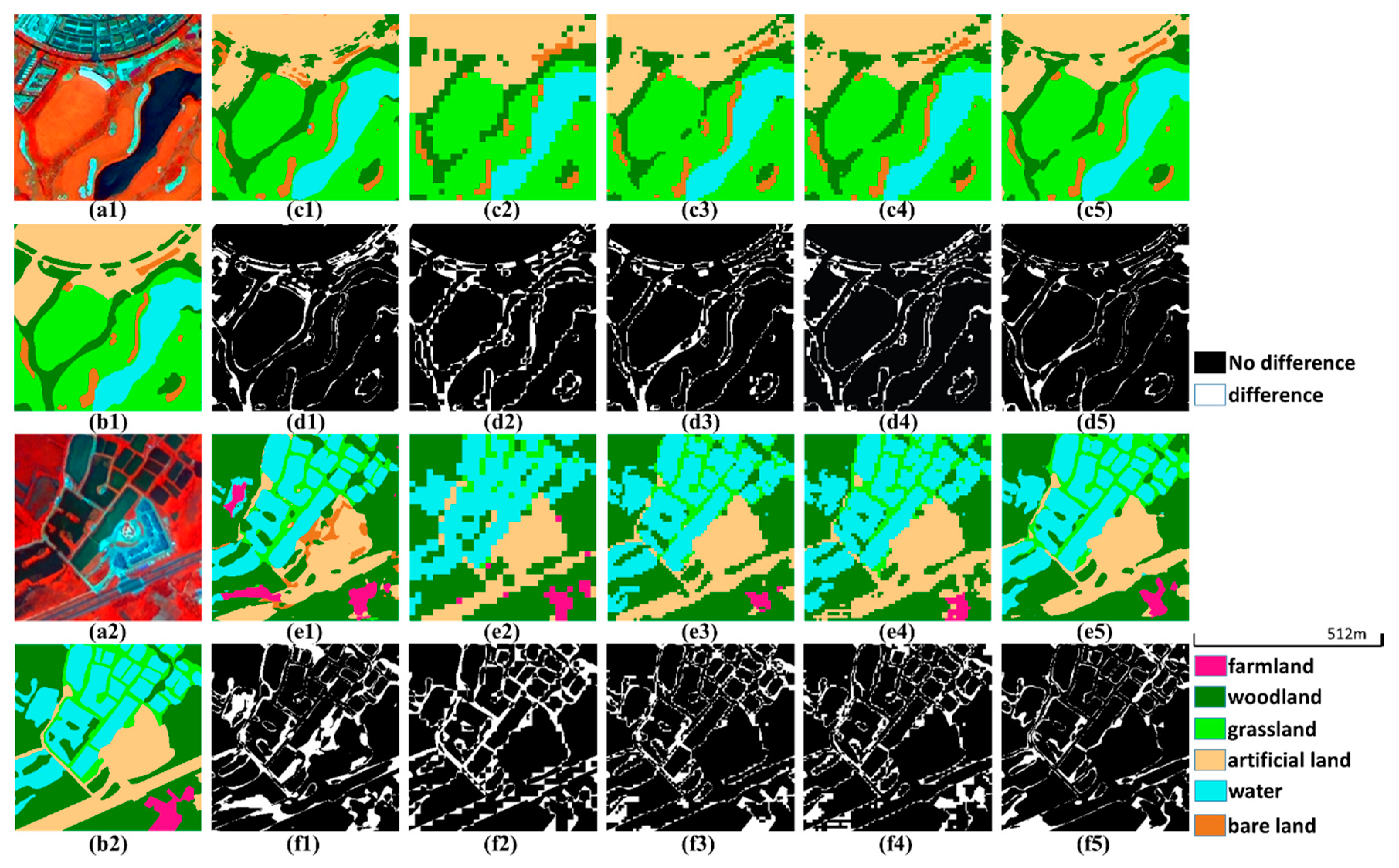
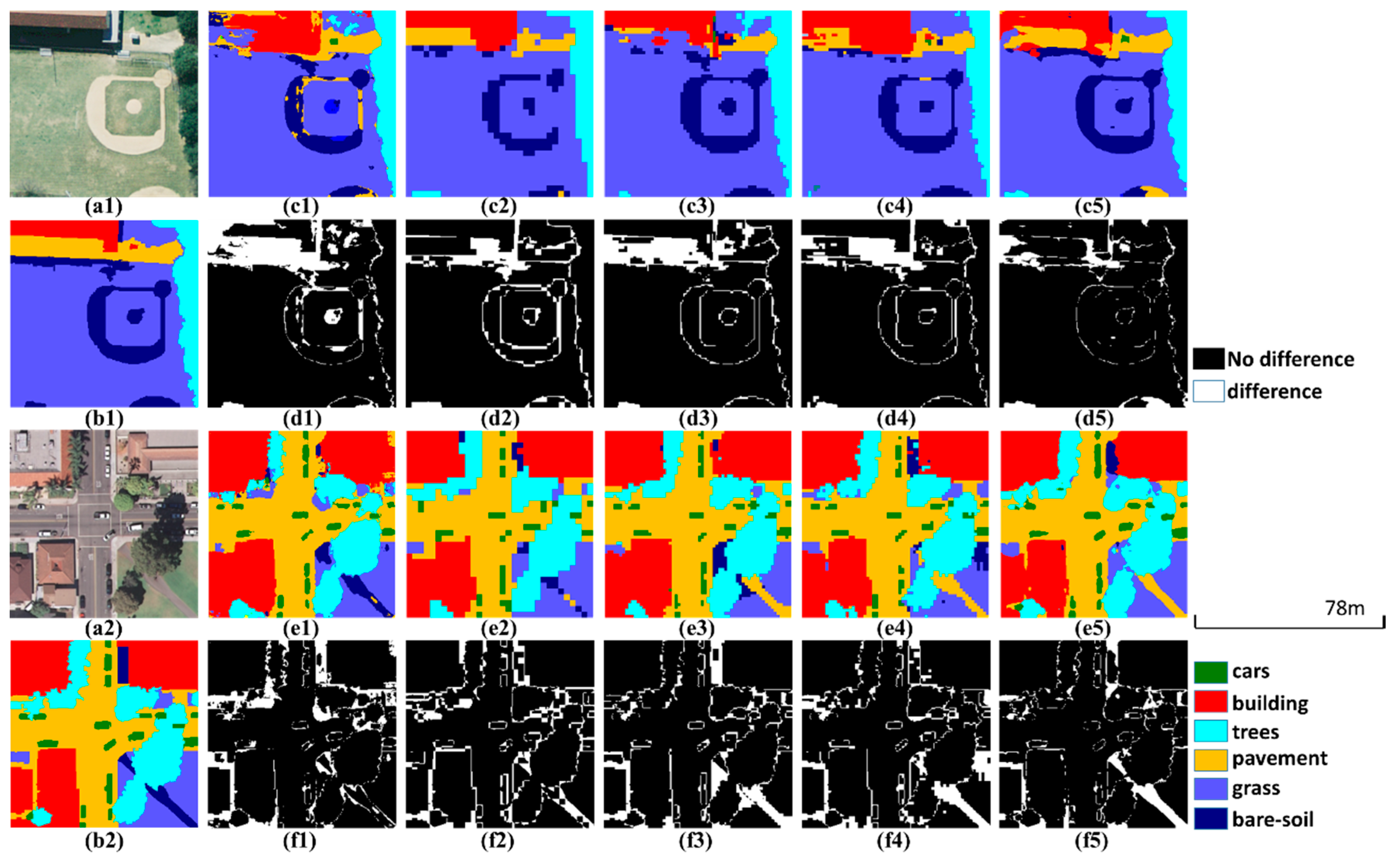
Figure 16.
Prediction examples in the validation set of the public dataset. (a1,a2) True color images. (b1,b2) Ground truth images. (c1–c5,e1–e5) Predictions of U-Net, PSPNet (ResNet-50), DeepLabv3+ (ResNet-50), U-Net (ResNet-50) and ResMANet. (d1–d5,f1–f5) Corresponding difference maps.
Figure 16.
Prediction examples in the validation set of the public dataset. (a1,a2) True color images. (b1,b2) Ground truth images. (c1–c5,e1–e5) Predictions of U-Net, PSPNet (ResNet-50), DeepLabv3+ (ResNet-50), U-Net (ResNet-50) and ResMANet. (d1–d5,f1–f5) Corresponding difference maps.
Table 1.
Basic parameters of the satellite imagery.
Table 1.
Basic parameters of the satellite imagery.
| Satellite | | B1 (μm) | B2 (μm) | B3 (μm) | B4 (μm) | Panchromatic (μm) |
|---|
| GF-1 | Wavelength | 0.45–0.52 | 0.52–0.59 | 0.63–0.69 | 0.77–0.89 | 0.45–0.90 |
| Resolution | 8 m | 2 m |
| GF-2 | Wavelength | 0.45–0.52 | 0.52–0.59 | 0.63–0.69 | 0.77–0.89 | 0.45–0.90 |
| Resolution | 4 m | 1 m |
| ZY-3 | Wavelength | 0.45–0.52 | 0.52–0.59 | 0.63–0.69 | 0.77–0.89 | 0.45–0.80 |
| Resolution | 6 m | 2 m |
Table 2.
Comparison of training and prediction efficiency on true color images.
Table 2.
Comparison of training and prediction efficiency on true color images.
| Nets | Training (Seconds/Epoch) | Prediction (Seconds/1,000,000 Pixel) |
|---|
| U-Net | 80 | 0.69 |
| PSPNet (ResNet-50) | 85 | 0.83 |
| DeepLabv3+ (ResNet-50) | 73 | 0.89 |
| U-Net (ResNet-50) | 50 | 0.63 |
| ResMANet | 74 | 0.85 |
Table 3.
Accuracy assessment of Hainan dataset A.
Table 3.
Accuracy assessment of Hainan dataset A.
| Nets | PA | UA | OA | MIoU |
|---|
| U-Net | 88.98% | 89.05% | 90.02% | 80.51% |
| PSPNet (ResNet-50) | 91.70% | 89.67% | 91.75% | 83.06% |
| DeepLabv3+ (ResNet-50) | 90.70% | 91.05% | 92.10% | 83.39% |
| U-Net (ResNet-50) | 91.03% | 89.84% | 91.51% | 82.71% |
| ResMANet (CEL) | 89.73% | 89.31% | 90.51% | 81.16% |
| ResMANet | 92.20% | 92.23% | 92.80% | 85.78% |
Table 4.
Comparison of training and prediction efficiency on multi-spectral data.
Table 4.
Comparison of training and prediction efficiency on multi-spectral data.
| Nets | Training (Seconds/Epoch) | Prediction (Seconds/1,000,000 Pixel) |
|---|
| U-Net | 35 | 0.68 |
| PSPNet (ResNet-50) | 37 | 0.79 |
| DeepLabv3+ (ResNet-50) | 32 | 0.88 |
| U-Net (ResNet-50) | 22 | 0.60 |
| ResMANet | 30 | 0.71 |
Table 5.
Accuracy assessment of Hainan dataset B.
Table 5.
Accuracy assessment of Hainan dataset B.
| Nets | PA | UA | OA | MIoU |
|---|
| U-Net | 88.28% | 83.22% | 90.00% | 75.47% |
| PSPNet (ResNet-50) | 88.47% | 86.67% | 90.95% | 78.15% |
| DeepLabv3+ (ResNet-50) | 89.50% | 87.43% | 91.83% | 79.60% |
| U-Net (ResNet-50) | 88.43% | 88.16% | 91.45% | 79.38% |
| ResMANet (CEL) | 89.83% | 87.58% | 92.08% | 80.00% |
| ResMANet | 91.10% | 90.02% | 93.17% | 82.85% |
Table 6.
Accuracy assessment of the public dataset results between methods.
Table 6.
Accuracy assessment of the public dataset results between methods.
| Nets | PA | UA | OA | MIoU |
|---|
| U-Net | 85.63% | 83.04% | 83.89% | 73.37% |
| PSPNet (ResNet-50) | 87.79% | 87.58% | 90.65% | 79.03% |
| DeepLabv3+ (ResNet-50) | 89.47% | 89.71% | 90.82% | 80.04% |
| U-Net (ResNet-50) | 87.86% | 85.26% | 88.41% | 76.79% |
| ResMANet | 90.97% | 90.90% | 91.52% | 83.75% |


