Deep Learning-Based Generation of Building Stock Data from Remote Sensing for Urban Heat Demand Modeling

 , and
, and
Abstract
:1. Introduction
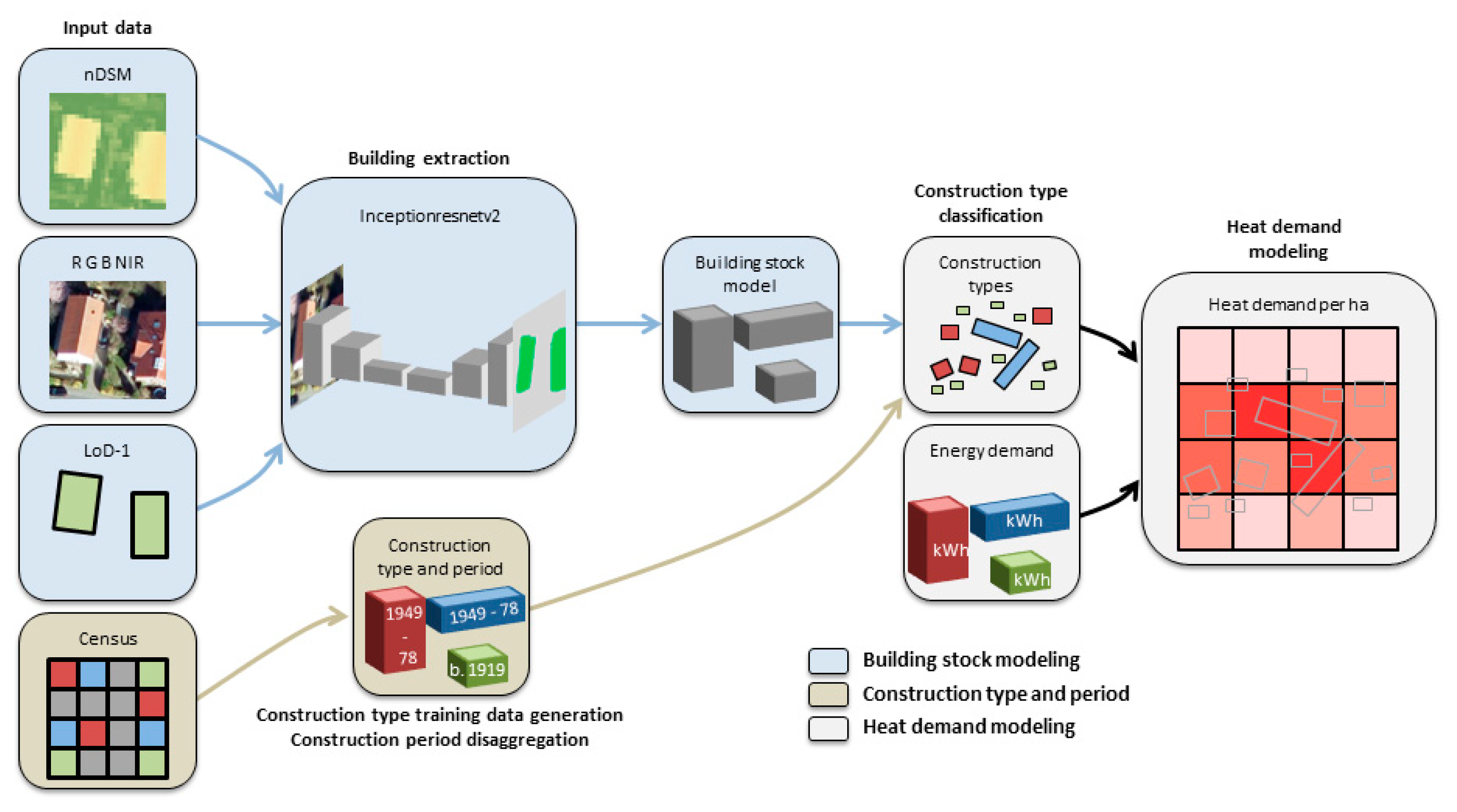
2. Data and Methods
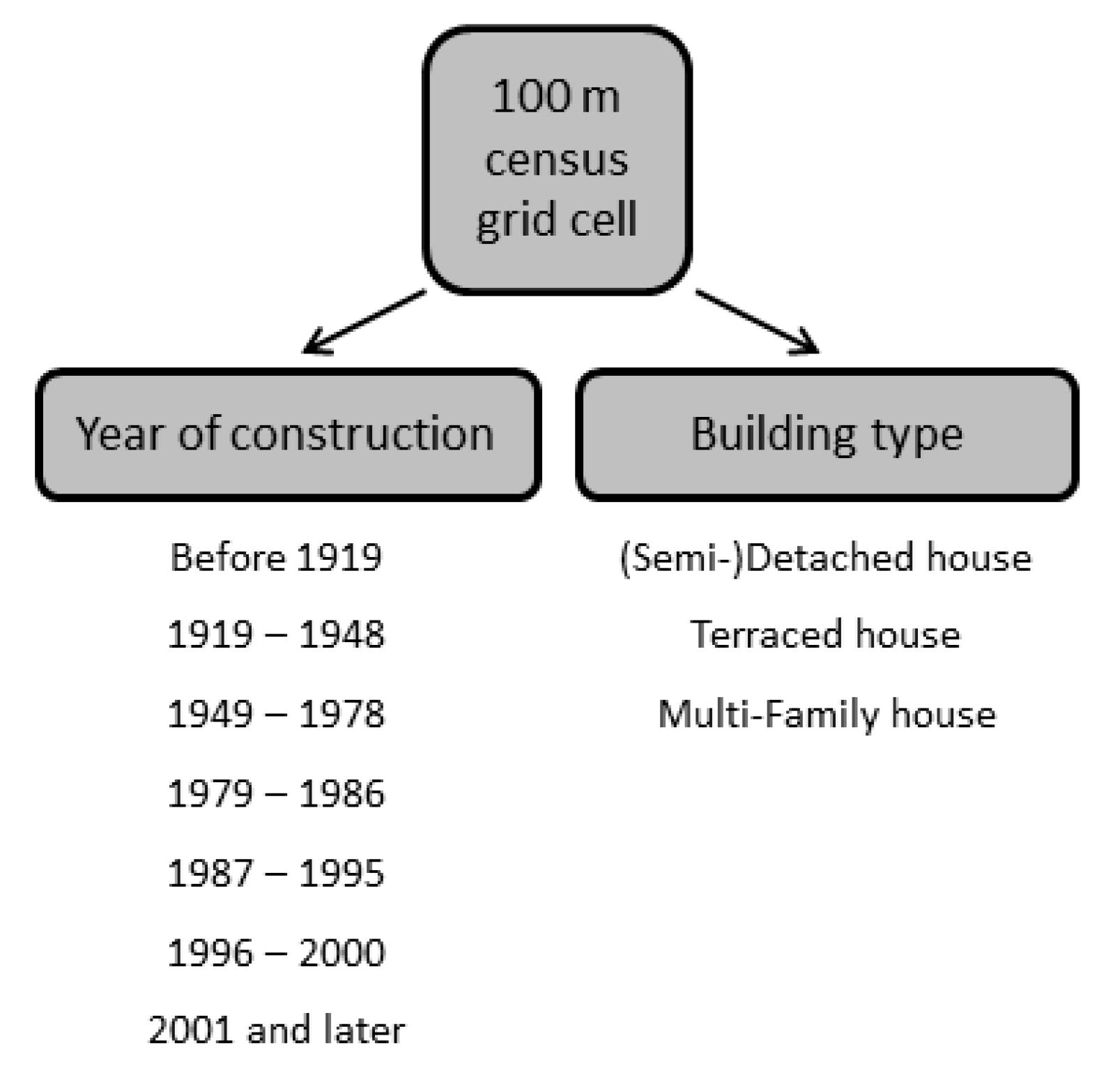
2.1. Data
2.2. Building Stock Modeling
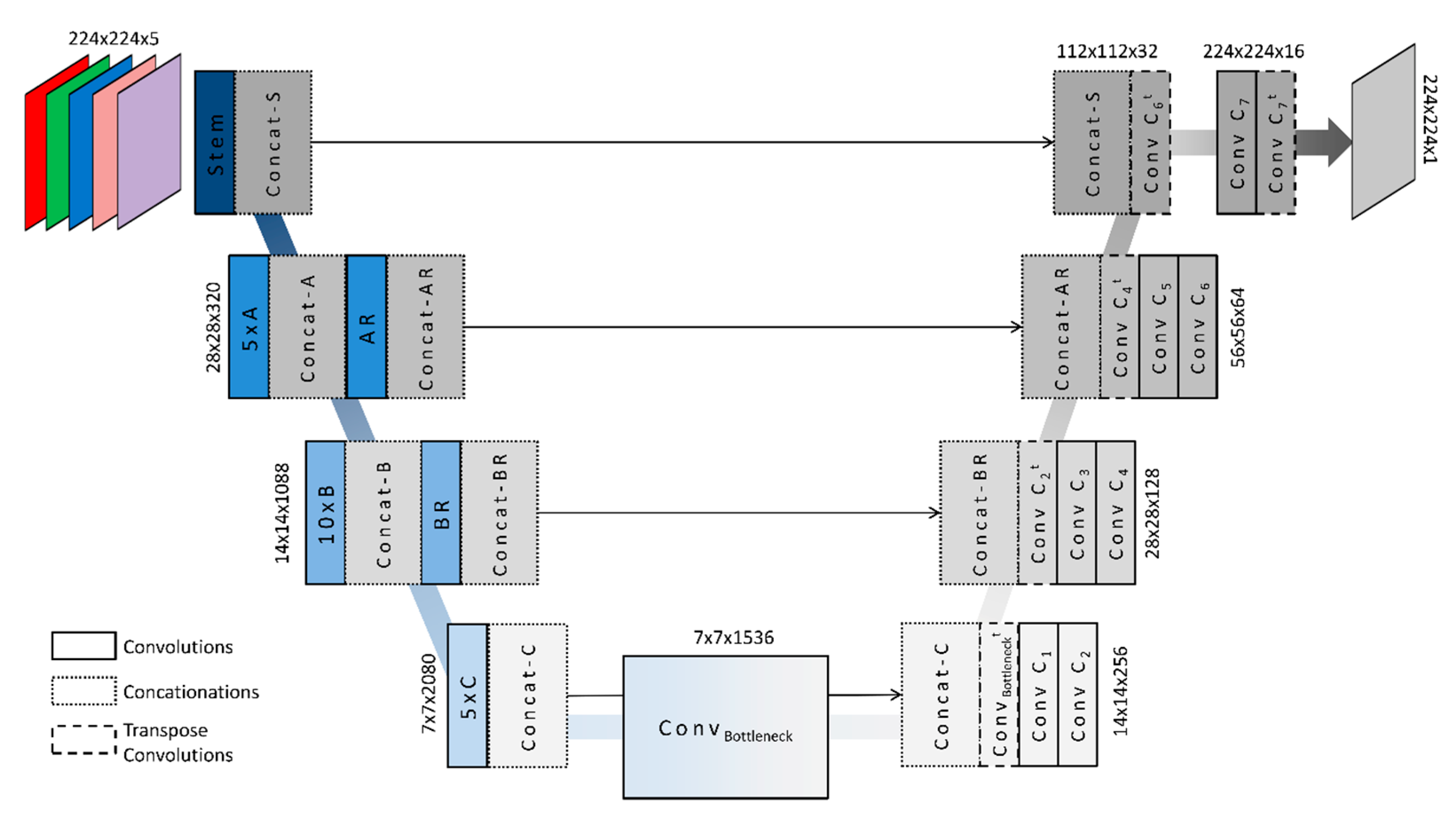
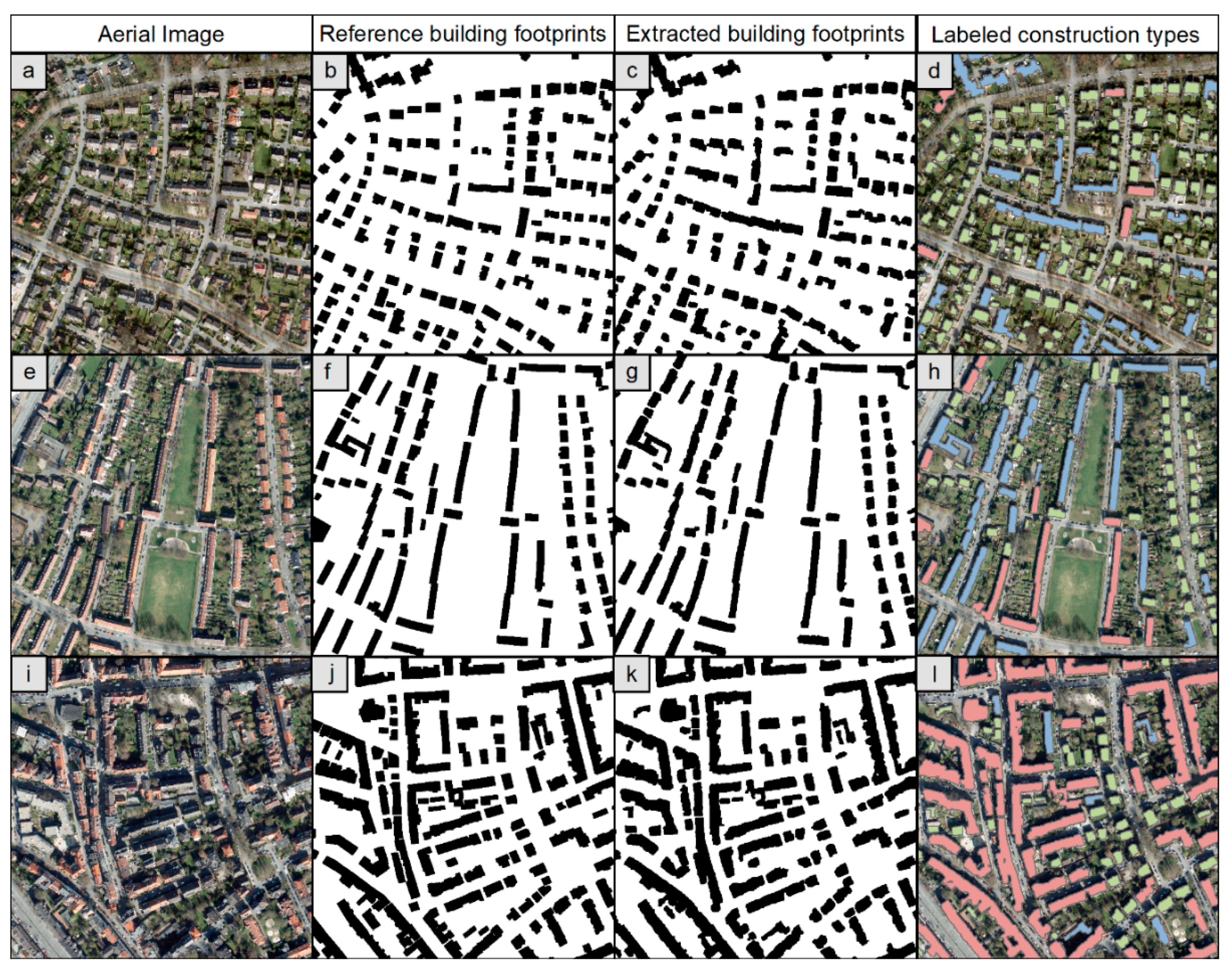
2.2.1. Building Extraction from Aerial Images Using Deep Learning
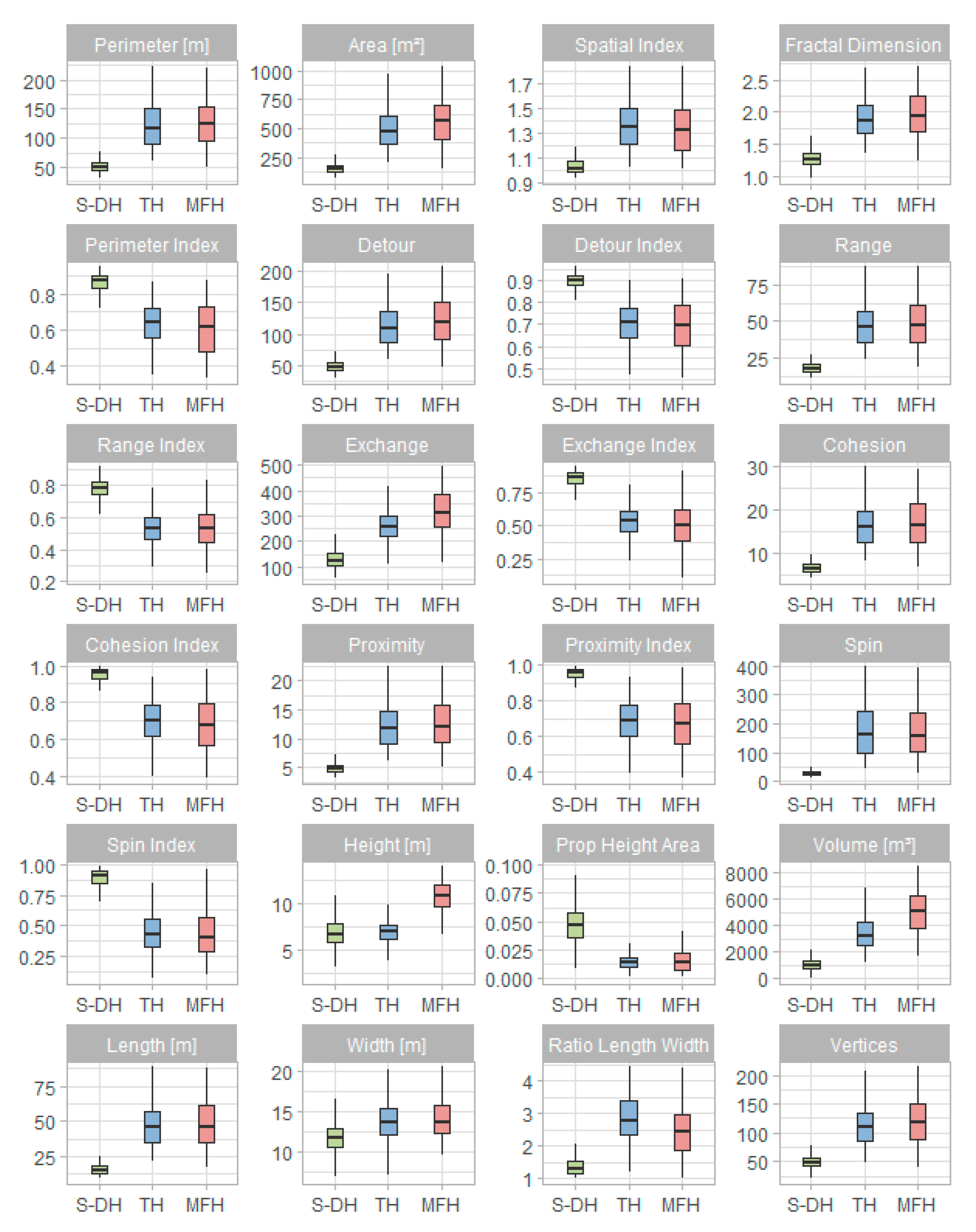
2.2.2. Building Geometry
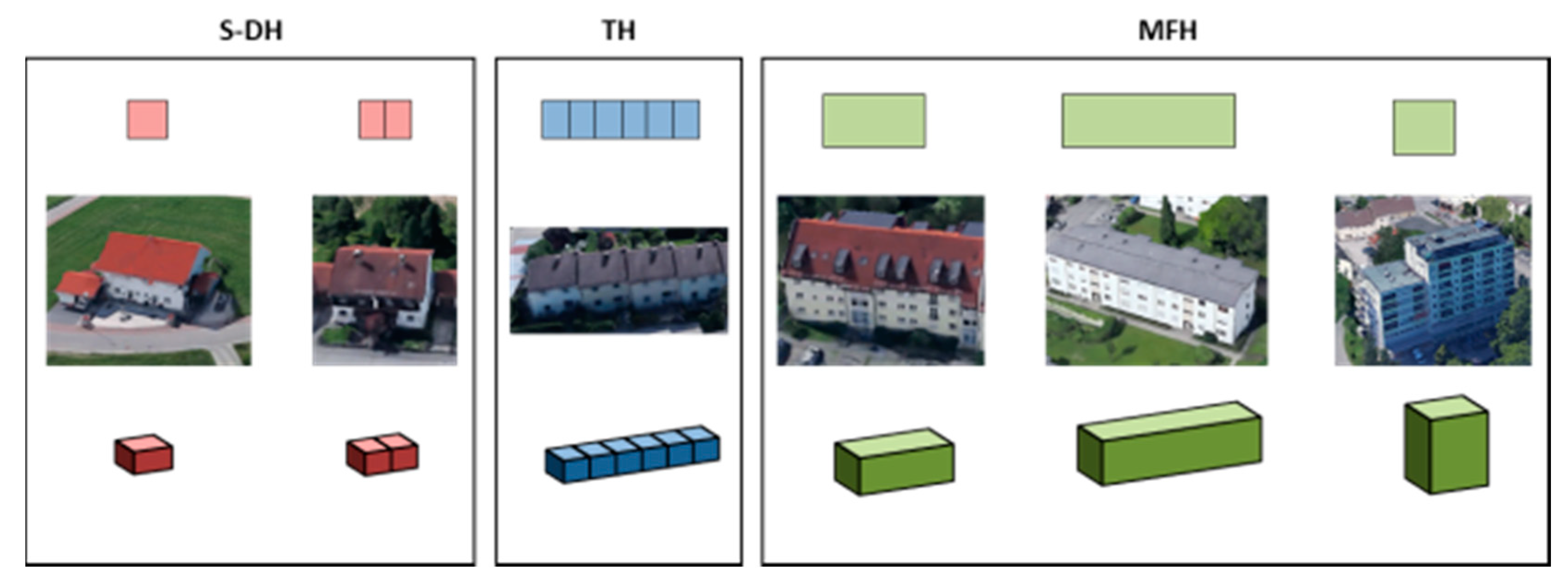
2.2.3. Semantic Labeling of the Construction Type
2.2.4. Disaggregation of the Construction Period
2.3. Building Heat Demand Modeling
3. Results
3.1. Building Stock Modeling
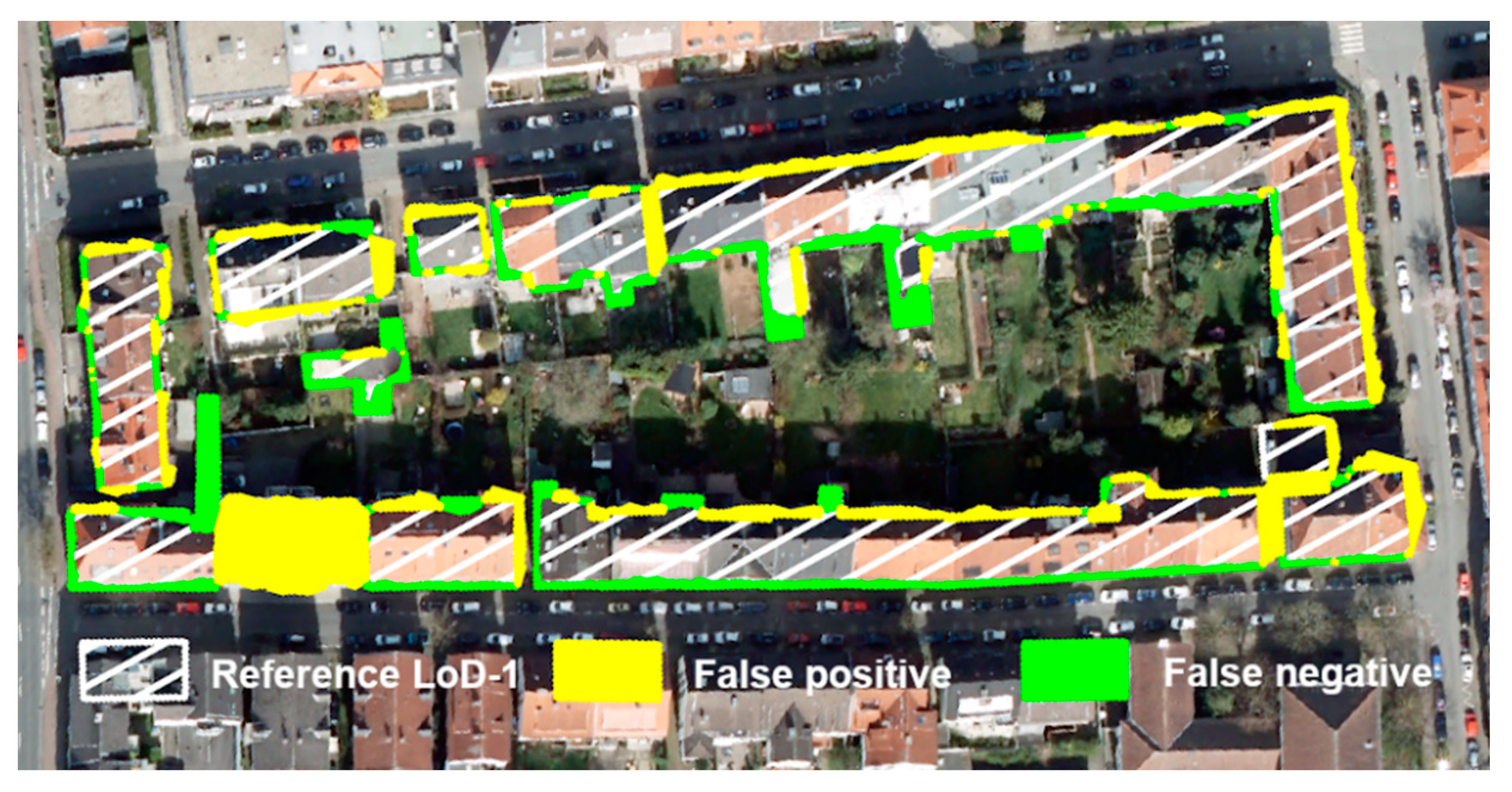
3.1.1. Building Extraction from Aerial Images Using U-net Inecptionresnetv2
3.1.2. Semantic Labeling of Construction Types
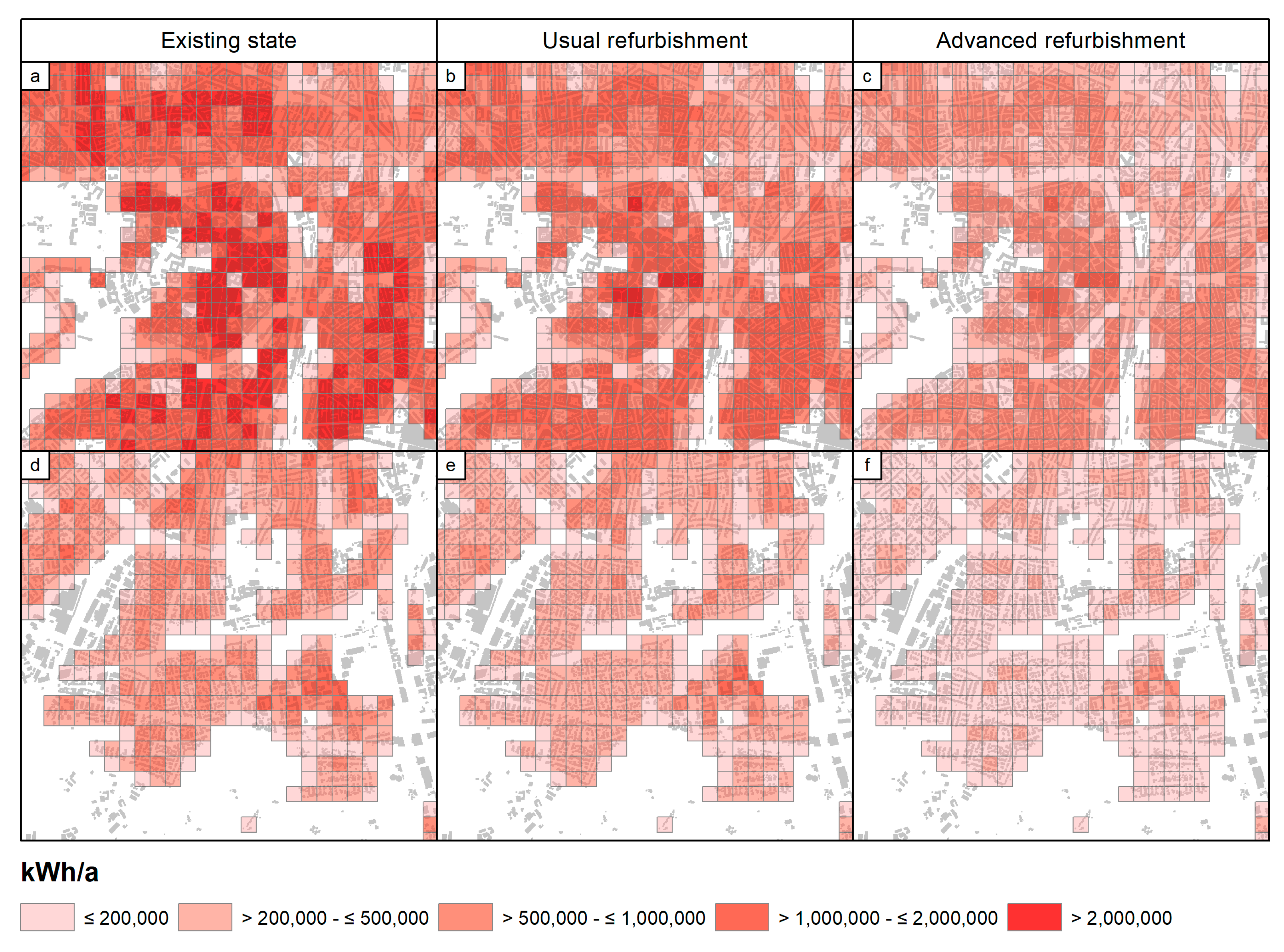
3.2. Heat Demand Modeling
3.2.1. Grid Level
3.2.2. City Scale
3.2.3. Construction Type and Construction Period
3.2.4. Comparison with Energy Atlas NRW
4. Discussion
5. Conclusions
Author Contributions
Funding
Institutional Review Board Statement
Informed Consent Statement
Data Availability Statement
Acknowledgments
Conflicts of Interest
References
- European Environment Agency. Trends and Projections in Europe 2015. Tracking Progress towards Europe’s Climate and Energy Targets; European Environment Agency: Luxembourg, 2015.
- Silva, M.; Oliveira, V.; Leal, V. Urban Form and Energy Demand: A Review of Energy-Relevant Urban Attributes. J. Plan. Lit. 2017, 32, 346–365. [Google Scholar] [CrossRef]
- BPIE—Buildings Performance Institute Europe. Renovating Germany’s Building Stock. An Economic Appraisal from the Investors’ Perspective. Available online: http://bpie.eu/wp-content/uploads/2016/02/BPIE_Renovating-Germany-s-Building-Stock-_EN_09.pdf (accessed on 24 November 2020).
- EC—European Commission. Building Stock Characteristics. Available online: https://ec.europa.eu/energy/en/eu-buildings-factsheets-topics-tree/building-stock-characteristics (accessed on 24 November 2020).
- Hong, T.; Chen, Y.; Luo, X.; Luo, N.; Lee, S.H. Ten Questions on Urban Building Energy Modeling. Build. Environ. 2020, 168, 106508. [Google Scholar] [CrossRef] [Green Version]
- Reinhart, C.F.; Cerezo Davila, C. Urban Building Energy Modeling—A Review of a Nascent Field. Build. Environ. 2016, 97, 196–202. [Google Scholar] [CrossRef] [Green Version]
- Chen, Y.; Hong, T.; Luo, X.; Hooper, B. Development of City Buildings Dataset for Urban Building Energy Modeling. Energy Build. 2019, 183, 252–265. [Google Scholar] [CrossRef] [Green Version]
- Sola, A.; Corchero, C.; Salom, J.; Sanmarti, M. Simulation Tools to Build Urban-Scale Energy Models: A Review. Energies 2018, 11, 3269. [Google Scholar] [CrossRef] [Green Version]
- Rosser, J.F.; Long, G.; Zakhary, S.; Boyd, D.S.; Mao, Y.; Robinson, D. Modelling Urban Housing Stocks for Building Energy Simulation Using CityGML EnergyADE. ISPRS Int. J. Geo-Inf. 2019, 8, 163. [Google Scholar] [CrossRef] [Green Version]
- Fonseca, J.A.; Nguyen, T.-A.; Schlueter, A.; Marechal, F. City Energy Analyst (CEA): Integrated Framework for Analysis and Optimization of Building Energy Systems in Neighborhoods and City Districts. Energy Build. 2016, 113, 202–226. [Google Scholar] [CrossRef]
- Estevam Schmiedt, J.; Cerra, D.; Dahlke, D.; Dill, S.; Ge, N.; Göttsche, J.; Haas, A.; Heiden, U.; Israel, M.; Kurz, F.; et al. Remote Sensing Techniques for Building Models and Energy Performance Studies of Buildings. Available online: https://www.researchgate.net/publication/318283747_Remote_sensing_techniques_for_building_models_and_energy_performance_studies_of_buildings (accessed on 24 November 2020).
- Mastrucci, A.; Baume, O.; Stazi, F.; Leopold, U. Estimating Energy Savings for the Residential Building Stock of an Entire City: A GIS-Based Statistical Downscaling Approach Applied to Rotterdam. Energy Build. 2014, 75, 358–367. [Google Scholar] [CrossRef]
- Österbring, M.; Mata, É.; Thuvander, L.; Mangold, M.; Johnsson, F.; Wallbaum, H. A Differentiated Description of Building-Stocks for a Georeferenced Urban Bottom-up Building-Stock Model. Energy Build. 2016, 120, 78–84. [Google Scholar] [CrossRef] [Green Version]
- Kaden, R.; Kolbe, T.H. City-Wide Total Energy Demand Estimation of Buildings Using Semantic 3D City Model and Statistical Data. ISPRS Ann. Photogramm. Remote Sens. Spatial Inf. Sci. 2013, II-2/W1, 163–171. [Google Scholar] [CrossRef] [Green Version]
- Ma, J.; Cheng, J.C.P. Estimation of the Building Energy Use Intensity in the Urban Scale by Integrating GIS and Big Data Technology. Appl. Energy 2016, 183, 182–192. [Google Scholar] [CrossRef]
- Evans, S.; Liddiard, R.; Steadman, P. 3DStock: A New Kind of Three-Dimensional Model of the Building Stock of England and Wales, for Use in Energy Analysis. Environ. Plan. B Urban Anal. City Sci. 2017, 44, 227–255. [Google Scholar] [CrossRef] [Green Version]
- Chen, Y.; Hong, T.; Piette, M.A. Automatic Generation and Simulation of Urban Building Energy Models Based on City Datasets for City-Scale Building Retrofit Analysis. Appl. Energy 2017, 205, 323–335. [Google Scholar] [CrossRef] [Green Version]
- Swan, L.G.; Ugursal, V.I. Modeling of End-Use Energy Consumption in the Residential Sector: A Review of Modeling Techniques. Renew. Sustain. Energy Rev. 2009, 13, 1819–1835. [Google Scholar] [CrossRef]
- Li, W.; Zhou, Y.; Cetin, K.; Eom, J.; Wang, Y.; Chen, G.; Zhang, X. Modeling Urban Building Energy Use: A Review of Modeling Approaches and Procedures. Energy 2017, 141, 2445–2457. [Google Scholar] [CrossRef]
- Johari, F.; Peronato, G.; Sadeghian, P.; Zhao, X.; Widén, J. Urban Building Energy Modeling: State of the Art and Future Prospects. Renew. Sustain. Energy Rev. 2020, 128, 109902. [Google Scholar] [CrossRef]
- Nouvel, R.; Mastrucci, A.; Leopold, U.; Baume, O.; Coors, V.; Eicker, U. Combining GIS-Based Statistical and Engineering Urban Heat Consumption Models: Towards a New Framework for Multi-Scale Policy Support. Energy Build. 2015, 107, 204–212. [Google Scholar] [CrossRef]
- Krüger, A.; Kolbe, T.H. Buildings Analysis for Urban Energy Planning Using Key Indicators on Virtual 3D City Models. Int. Arch. Photogramm. Remote Sens. Spatial Inf. Sci. 2012, XXXIX-B2, 145–150. [Google Scholar] [CrossRef] [Green Version]
- Beck, A.; Long, G.; Boyd, D.S.; Rosser, J.F.; Morley, J.; Duffield, R.; Sanderson, M.; Robinson, D. Automated Classification Metrics for Energy Modelling of Residential Buildings in the UK with Open Algorithms. Environ. Plan. B Urban Anal. City Sci. 2020, 47, 45–64. [Google Scholar] [CrossRef]
- Aksoezen, M.; Daniel, M.; Hassler, U.; Kohler, N. Building Age as an Indicator for Energy Consumption. Energy Build. 2015, 87, 74–86. [Google Scholar] [CrossRef]
- Alhamwi, A.; Medjroubi, W.; Vogt, T.; Agert, C. OpenStreetMap Data in Modeling the Urban Energy Infrastructure: A First Assessment and Analysis. In Proceedings of the 9th International Conference on Applied Energy, ICAE2017, Cardiff, UK, 21–24 August 2017. [Google Scholar]
- LeCun, Y.; Bengio, Y.; Hinton, G. Deep Learning. Nature 2015, 521, 436–444. [Google Scholar] [CrossRef] [PubMed]
- Zhu, X.X.; Tuia, D.; Mou, L.; Xia, G.-S.; Zhang, L.; Xu, F.; Fraundorfer, F. Deep Learning in Remote Sensing: A Comprehensive Review and List of Resources. IEEE Geosci. Remote Sens. Mag. 2017, 5, 8–36. [Google Scholar] [CrossRef] [Green Version]
- Wurm, M.; Stark, T.; Zhu, X.X.; Weigand, M.; Taubenböck, H. Semantic Segmentation of Slums in Satellite Images Using Transfer Learning on Fully Convolutional Neural Networks. ISPRS J. Photogramm. Remote Sens. 2019, 150, 59–69. [Google Scholar] [CrossRef]
- Stiller, D.; Stark, T.; Wurm, M.; Dech, S.; Taubenbock, H. Large-Scale Building Extraction in Very High-Resolution Aerial Imagery Using Mask R-CNN. In Proceedings of the 2019 Joint Urban Remote Sensing Event (JURSE), Vannes, France, 22–24 May 2019; pp. 1–4. [Google Scholar]
- Wu, G.; Shao, X.; Guo, Z.; Chen, Q.; Yuan, W.; Shi, X.; Xu, Y.; Shibasaki, R. Automatic Building Segmentation of Aerial Imagery Using Multi-Constraint Fully Convolutional Networks. Remote Sens. 2018, 10, 407. [Google Scholar] [CrossRef] [Green Version]
- Marmanis, D.; Schindler, K.; Wegner, J.D.; Galliani, S.; Datcu, M.; Stilla, U. Classification with an Edge: Improving Semantic Image Segmentation with Boundary Detection. ISPRS J. Photogramm. Remote Sens. 2018, 135, 158–172. [Google Scholar] [CrossRef] [Green Version]
- Yi, Y.; Zhang, Z.; Zhang, W.; Zhang, C.; Li, W.; Zhao, T. Semantic Segmentation of Urban Buildings from VHR Remote Sensing Imagery Using a Deep Convolutional Neural Network. Remote Sens. 2019, 11, 1774. [Google Scholar] [CrossRef] [Green Version]
- Microsoft US Building Footprints. Available online: https://github.com/Microsoft/USBuildingFootprints (accessed on 24 November 2020).
- Lin, G.; Milan, A.; Shen, C.; Reid, I. RefineNet: Multi-Path Refinement Networks for High-Resolution Semantic Segmentation. arXiv 2016, arXiv:1611.06612. [Google Scholar]
- Huang, J.; Zhang, X.; Xin, Q.; Sun, Y.; Zhang, P. Automatic Building Extraction from High-Resolution Aerial Images and LiDAR Data Using Gated Residual Refinement Network. ISPRS J. Photogramm. Remote Sens. 2019, 151, 91–105. [Google Scholar] [CrossRef]
- Bittner, K.; Cui, S.; Reinartz, P. Building Extraction from Remote Sensing Data Using Fully Convolutional Networks. Int. Arch. Photogramm. Remote Sens. Spatial Inf. Sci. 2017, XLII-1/W1, 481–486. [Google Scholar] [CrossRef] [Green Version]
- Henn, A.; Römer, C.; Gröger, G.; Plümer, L. Automatic Classification of Building Types in 3D City Models: Using SVMs for Semantic Enrichment of Low Resolution Building Data. Geoinformatica 2012, 16, 281–306. [Google Scholar] [CrossRef]
- Wurm, M.; Schmitt, A.; Taubenbock, H. Building Types’ Classification Using Shape-Based Features and Linear Discriminant Functions. IEEE J. Sel. Top. Appl. Earth Obs. Remote Sens. 2016, 9, 1901–1912. [Google Scholar] [CrossRef]
- Belgiu, M.; Tomljenovic, I.; Lampoltshammer, T.; Blaschke, T.; Höfle, B. Ontology-Based Classification of Building Types Detected from Airborne Laser Scanning Data. Remote Sens. 2014, 6, 1347–1366. [Google Scholar] [CrossRef] [Green Version]
- Du, S.; Zhang, F.; Zhang, X. Semantic Classification of Urban Buildings Combining VHR Image and GIS Data: An Improved Random Forest Approach. ISPRS J. Photogramm. Remote Sens. 2015, 105, 107–119. [Google Scholar] [CrossRef]
- Aubrecht, C.; Steinnocher, K.; Hollaus, M.; Wagner, W. Integrating Earth Observation and GIScience for High Resolution Spatial and Functional Modeling of Urban Land Use. Comput. Environ. Urban Syst. 2009, 33, 15–25. [Google Scholar] [CrossRef]
- Monien, D.; Strzalka, A.; Koukofikis, A.; Coors, V.; Eicker, U. Comparison of Building Modelling Assumptions and Methods for Urban Scale Heat Demand Forecasting. Future Cities Environ. 2017, 3, 2. [Google Scholar] [CrossRef]
- Zirak, M.; Weiler, V.; Hein, M.; Eicker, U. Urban Models Enrichment for Energy Applications: Challenges in Energy Simulation Using Different Data Sources for Building Age Information. Energy 2020, 190, 116292. [Google Scholar] [CrossRef]
- Long, J.; Shelhamer, E.; Darrell, T. Fully Convolutional Networks for Semantic Segmentation. arXiv 2015, arXiv:1411.4038. [Google Scholar]
- Ronneberger, O.; Fischer, P.; Brox, T. U-Net: Convolutional Networks for Biomedical Image Segmentation. arXiv 2015, arXiv:1505.04597. [Google Scholar]
- Simonyan, K.; Zisserman, A. Very Deep Convolutional Networks for Large-Scale Image Recognition. arXiv 2015, arXiv:1409.1556. [Google Scholar]
- Szegedy, C.; Liu, W.; Jia, Y.; Sermanet, P.; Reed, S.; Anguelov, D.; Erhan, D.; Vanhoucke, V.; Rabinovich, A. Going Deeper with Convolutions. arXiv 2014, arXiv:1409.4842. [Google Scholar]
- Lin, M.; Chen, Q.; Yan, S. Network in Network. arXiv 2014, arXiv:1312.4400. [Google Scholar]
- Szegedy, C.; Vanhoucke, V.; Ioffe, S.; Shlens, J.; Wojna, Z. Rethinking the Inception Architecture for Computer Vision. arXiv 2015, arXiv:1512.00567. [Google Scholar]
- He, K.; Zhang, X.; Ren, S.; Sun, J. Deep Residual Learning for Image Recognition. In Proceedings of the 2016 IEEE Conference on Computer Vision and Pattern Recognition (CVPR), Las Vegas, NV, USA, 27–30 June 2016; pp. 770–778. [Google Scholar]
- Kingma, D.P.; Ba, J. Adam: A Method for Stochastic Optimization. arXiv 2017, arXiv:1412.6980. [Google Scholar]
- Serra, J. Image Analysis and Mathematical Morphology; Academic Press, Inc.: Orlando, FL, USA, 1982. [Google Scholar]
- Wurm, M.; Taubenböck, H.; Schardt, M.; Esch, T.; Dech, S. Object-Based Image Information Fusion Using Multisensor Earth Observation Data over Urban Areas. Int. J. Image Data Fusion 2011, 2, 121–147. [Google Scholar] [CrossRef]
- Wurm, M.; Goebel, J.; Wagner, G.G.; Weigand, M.; Dech, S.; Taubenböck, H. Inferring Floor Area Ratio Thresholds for the Delineation of City Centers Based on Cognitive Perception. Environ. Plan. B Urban Anal. City Sci. 2019, 239980831986934. [Google Scholar] [CrossRef] [Green Version]
- Breiman, L. Random Forests. Mach. Learn. 2001, 45, 5–32. [Google Scholar] [CrossRef] [Green Version]
- Fernandez-Delgado, M.; Cernadaseva, E.; Barro, S.; Amorim, D. Do We Need Hundreds of Classifiers to Solve Real World Classification Problems? JMRS 2014, 15, 3133–3181. [Google Scholar]
- Angel, S.; Parent, J.; Civco, D.L. Ten Compactness Properties of Circles: Measuring Shape in Geography: Ten Compactness Properties of Circles. Can. Geogr. Géographe Can. 2010, 54, 441–461. [Google Scholar] [CrossRef]
- Droin, A.; Wurm, M.; Sulzer, W. Semantic Labelling of Building Types. A Comparison of Two Approaches Using Random Forest and Deep Learning. Available online: https://www.researchgate.net/publication/339800032_Semantic_labelling_of_building_types_A_comparison_of_two_approaches_using_Random_Forest_and_Deep_Learning (accessed on 24 November 2020).
- Garbasevschi, O.; Estevam Schmiedt, J.; Verma, T.; Lefter, I.; Korthals Altes, W.K.; Droin, A.; Schiricke, B.; Wurm, M. Spatial Factors Influencing Building Age Prediction and Implications for Urban Energy Modelling. Comput. Environ. Urban Syst. under review.
- IWU—Institut für Wohnen und Umwelt (German Institute for Housing and Environment). Deutsche Gebäudetypologie. Beispielhafte Maßnahmen Zur Verbesserung Der Energieeffizienz von Typischen Wohngebäuden—Zweite Erweirter Auflage; Institut für Wohnen und Umwelt: Darmstadt, Germany, 2015. [Google Scholar]
- Loga, T.; Stein, B.; Diefenbach, N. TABULA Building Typologies in 20 European Countries—Making Energy-Related Features of Residential Building Stocks Comparable. Energy Build. 2016, 132, 4–12. [Google Scholar] [CrossRef]
- BBSR—Bundesinstitut für Bau-, Stadt- und Raumforschung. Thermal Insulation Ordinance 1977. Available online: https://www.bbsr-energieeinsparung.de/EnEVPortal/EN/Archive/ThermalInsulation/1977/1977_node.html (accessed on 24 November 2020).
- Stiller, D.; Wurm, M.; Stark, T.; dAngelo, P.; Stebner, K.; Dech, S.; Taubenbock, H. Spatial Parameters for Transportation: A Multi-Modal Approach for Modelling the Urban Spatial Structure Using Deep Learning and Remote Sensing. J. Transp. Land Use, under review.
- Rosser, J.F.; Boyd, D.S.; Long, G.; Zakhary, S.; Mao, Y.; Robinson, D. Predicting Residential Building Age from Map Data. Comput. Environ. Urban Syst. 2019, 73, 56–67. [Google Scholar] [CrossRef] [Green Version]
- Wang, Z.; Crawley, J.; Li, F.G.N.; Lowe, R. Sizing of District Heating Systems Based on Smart Meter Data: Quantifying the Aggregated Domestic Energy Demand and Demand Diversity in the UK. Energy 2020, 193, 116780. [Google Scholar] [CrossRef]
- Ballarini, I.; Corgnati, S.P.; Corrado, V. Use of Reference Buildings to Assess the Energy Saving Potentials of the Residential Building Stock: The Experience of TABULA Project. Energy Policy 2014, 68, 273–284. [Google Scholar] [CrossRef]


| Name | Date | Granularity | Source | Use |
|---|---|---|---|---|
| Digital Orthophoto (DOP) | 2017 | 0.1 m | https://www.opengeodata.nrw.de | Building stock model |
| Digital Elevation Model (DEM) | 2019 | 1 m | https://www.opengeodata.nrw.de | Building stock model |
| Digital Surface Model (DSM) | 2012 | 1 m | https://www.opengeodata.nrw.de | Building stock model |
| 3D building model (LoD1) | 2015 | Area + height | https://www.opengeodata.nrw.de | Validation |
| Urban Land-use (DLM-DE) | 2015 | Urban blocks | https://www.opengeodata.nrw.de | Use type |
| Census data | 2011 | 100 m grid cells | https://www.zensus2011.de | Construction period |
| Reference heat demand | 2011 | Construction typeand period | https://www.iwu.de | Heat demand modeling |
| Energy Atlas | 2016 | 100 m grid cells | https://www.energieatlas.nrw.de | Validation |
| Name | Short Description | Name | Short Description |
|---|---|---|---|
| Perimeter (m) | Length of building outline | Cohesion | Average Euclidean distance between 30 randomly selected interior points |
| Area (m2) | Building footprint area | Cohesion Index | Normalized cohesion using the equal area circle radius and a constant |
| Height (m) | Measured height | Proximity | Average Euclidean distance from all interior points to the centroid |
| Shape Index | Proportion between perimeter and approximated square with equal area | Proximity Index | Normalized proximity using two thirds of the equal area radius |
| Fractal Dimension | Proportion between area and perimeter | Spin | Average of the square of Euclidean distances between all interior points and the centroid |
| Perimeter Index | Proportion of perimeter of shape to perimeter of circle with equal area | Spin Index | Normalized spin using 0.5 ∗ squared radius of the equal area circle |
| Detour | Perimeter of the convex hull | Height Area | Proportion between height and area |
| Detour Index | Normalized detour using the perimeter of the equal area circle | Volume (m3) | The volume of the building |
| Range | Longest distance between two vertex points of the building | Length (m) | The length of the bounding box of the building |
| Range Index | Normalized range using two times the diameter of the equal area circle | Width (m) | Width of the bounding box |
| Exchange | Shared area of the building footprint and the equal area circle with the same centroid | Length Width | Ratio between length and width of the bounding box |
| Exchange Index | Normalized exchange dividing the exchange area by the shape area | Vertices | Number of vertices of the building |
| Existing State | Usual Refurbishment | Advanced Refurbishment | |||||||
|---|---|---|---|---|---|---|---|---|---|
| Construction Year | S-DH | TH | MFH | S-DH | TH | MFH | S-DH | TH | MFH |
| before 1919 | 207.4 | 184.7 | 200.2 | 129.2 | 127.5 | 124.8 | 56.5 | 54.7 | 55.7 |
| 1919–1948 | 192.0 | 167.2 | 200.0 | 118.0 | 104.0 | 117.6 | 53.8 | 46.4 | 59.2 |
| 1949–1978 | 198.4 | 160 | 175.8 | 141.6 | 106.2 | 108.2 | 68.2 | 48.8 | 55.7 |
| 1979–1986 | 154.4 | 158.3 | 156.8 | 108.9 | 120.9 | 103.0 | 47.6 | 55.2 | 52.7 |
| 1987–1995 | 165.3 | 132.5 | 160.1 | 129.2 | 105.6 | 107.3 | 61.4 | 44.9 | 55.5 |
| 1996–2000 | 145.8 | 112.9 | 126.5 | 125.5 | 96.5 | 97.1 | 62.9 | 43.0 | 49.3 |
| after 2001 | 112.8 | 104.0 | 91.8 | 99.0 | 95.6 | 81.1 | 59.2 | 54.5 | 46.3 |
| Reference | ||||
|---|---|---|---|---|
| S-DH | TH | MFH | ||
| Prediction | S-DH | 344 | 6 | 1 |
| TH | 6 | 104 | 4 | |
| MFH | 3 | 4 | 117 | |
Publisher’s Note: MDPI stays neutral with regard to jurisdictional claims in published maps and institutional affiliations. |
© 2021 by the authors. Licensee MDPI, Basel, Switzerland. This article is an open access article distributed under the terms and conditions of the Creative Commons Attribution (CC BY) license (http://creativecommons.org/licenses/by/4.0/).
Share and Cite
Wurm, M.; Droin, A.; Stark, T.; Geiß, C.; Sulzer, W.; Taubenböck, H. Deep Learning-Based Generation of Building Stock Data from Remote Sensing for Urban Heat Demand Modeling. ISPRS Int. J. Geo-Inf. 2021, 10, 23. https://0-doi-org.brum.beds.ac.uk/10.3390/ijgi10010023
Wurm M, Droin A, Stark T, Geiß C, Sulzer W, Taubenböck H. Deep Learning-Based Generation of Building Stock Data from Remote Sensing for Urban Heat Demand Modeling. ISPRS International Journal of Geo-Information. 2021; 10(1):23. https://0-doi-org.brum.beds.ac.uk/10.3390/ijgi10010023
Chicago/Turabian StyleWurm, Michael, Ariane Droin, Thomas Stark, Christian Geiß, Wolfgang Sulzer, and Hannes Taubenböck. 2021. "Deep Learning-Based Generation of Building Stock Data from Remote Sensing for Urban Heat Demand Modeling" ISPRS International Journal of Geo-Information 10, no. 1: 23. https://0-doi-org.brum.beds.ac.uk/10.3390/ijgi10010023