Article

Impact of Urban Land-Cover Changes on the Spatial-Temporal Land Surface Temperature in a Tropical City of Mexico

by
Erika Betzabeth Palafox-Juárez
1,
Jorge Omar López-Martínez
2,*,
José Luis Hernández-Stefanoni
3 and
Héctor Hernández-Nuñez
4
1
CONACYT-El Colegio de la Frontera Sur, Unidad Chetumal, Estación para la Recepción de Información Satelital (ERIS), Av. Centenario Km. 5.5 C.P., Chetumal, Quintana Roo 77014, Mexico
2
CONACYT-El Colegio de la Frontera Sur, unidad Chetumal, Departamento de Agricultura, Sociedad y Ambiente, Av. Centenario Km. 5.5 C.P., Chetumal, Quintana Roo 77014, Mexico
3
Centro de Investigación Científica de Yucatán A.C., Unidad de Recursos Naturales, Calle 43 130, Colonia Chuburna de Hidalgo, C.P., Mérida, Yucatán 97200, Mexico
4
Centro de Investigación y de Estudios Avanzados del Instituto Politécnico Nacional, Carretera Antigua a Progreso km 6 S/N. C.P., Mérida, Yucatán 97310, Mexico
*
Author to whom correspondence should be addressed.
ISPRS Int. J. Geo-Inf. 2021, 10(2), 76; https://0-doi-org.brum.beds.ac.uk/10.3390/ijgi10020076
Submission received: 31 December 2020 / Revised: 29 January 2021 / Accepted: 8 February 2021 / Published: 13 February 2021

Abstract

:
Climate change has severe consequences on ecosystem processes, as well as on people’s quality of life. It has been suggested that the loss of vegetation cover increases the land surface temperature (LST) due to modifications in biogeochemical patterns, generating a phenomenon known as “urban heat island” (UHI). The aim of this work was to analyze the effects of urban land-cover changes on the spatiotemporal variation of surface temperature in the tropical city of Mérida, Mexico. To find these effects we used both detected land-cover changes as well as variations of the Normalized Difference Vegetation Index (NDVI). Mérida is ranked worldwide as one of the best cities to live due to its quality of life. Data from satellite images of Landsat were analyzed to calculate land use change (LUC), LST, and NDVI. LST increased ca. 4 °C in the dry season and 3 °C in the wet season because of the LUC. In addition, a positive relationship between the LST and the NDVI was observed mainly in the dry season. The results confirm an increase in the LST as a consequence of the loss of vegetation cover, which favors the urban heat island phenomenon.

1. Introduction

Urbanization is a global phenomenon widely associated with processes of land-cover change with negative consequences on the ecosystem functioning. Particularly, under climate change context, the consequences of urbanization on local weather variables (e.g., rainfall intensity and surface temperature) are increasingly important [1]. During the last three decades, the world’s urbanization has seen a severe transformation in urban landscapes [2]. According to a United Nations report [3], urban populations increased from 751 million people in 1950 to 4.2 billion in 2018. In this context, Latin America is the second region, after Africa, with the highest rate of urban growth, approximately 133 million people live in urban areas. In Mexico, approximately 90 million people (77% of the population) live in urban areas [4].
One of the main negative consequences of the increase in urban infrastructure is the creation of impermeable and dry surfaces that reduce the availability of moisture for natural evapotranspiration from the soil [5], causing a phenomenon called urban heat island UHI [5,6,7]. The UHI is defined as the difference in temperature between the hottest sector of the city and the non-urban, or rural, space surrounding the city at a given time and is influenced by climatic factors (solar radiation, wind and clouds, for example), and the variability in structures and materials typical of an urban area [6,7,8] define seven main causes of urban heat island: (1) Anthropogenic heat production (combustion, etc.). (2) Reduction of latent heat loss (low degree of evapotranspiration) due to the use of impermeable surfaces (cement, concrete, pavements, etc.), efficient drainage systems, and scarce vegetation. (3) Low sensible heat loss due to reduced wind speed. (4) Greater absorption of solar radiation trapped by urban canyons. (5) Decrease in outgoing long-wave radiation due to a low sky vision factor. (6) Greater heat storage in building materials during the day due to their high capacity to retain heat and release it at night. (7) Re-emission of long-wave atmospheric radiation to the ground resulting from air pollution (greenhouse effect).
Several studies have shown the importance of landscape composition and UHI phenomenon, for example, a study in Washington showed average differences of about 10.8 °C between urban and rural areas [9]. Also, it has been observed that UHI phenomenon tends to have severe effects towards the interior of urban sites, dissipating towards rural areas [10,11,12]. Because of the decrease in evapotranspiration due to the construction of infrastructure, UHI phenomenon has consequences on climate variables on a local or regional scale. For example, variations in rainfall patterns [13] and surface temperature have been observed modifying the environmental and regional climate by remodeling the boundary layer and Earth–atmosphere circulation [14]. However, few studies have been carried out in tropical cities to understand the effect of land use change on land surface temperature (LST) and heat islands, particularly in ecosystems with marked seasonality. Seasonality represents one of the major sources of natural variation in the climate and is known to drive cycles of plant productivity in many ecosystems [15,16,17]. It has been widely observed that interannual variations in precipitation have direct implications on evapotranspiration, as well as on soil moisture [18] and solar radiation [19]. In addition, it has implications for the phenology of vegetation, affecting the roughness of the Earth’s surface, the albedo, and the interception of water [20], which leads to variations in LST.
The UHI phenomenon can be addressed from two approaches, atmospheric and surface [21,22]. Atmospheric UHI is assessed using data from meteorological stations, while surface UHI is studied using remote sensing thermal infrared (TIR) data [23,24]. In recent years, remote sensing techniques have been successfully applied to detect UHI phenomenon in several regions, analyze urban surface radiation, estimate surface heat balance, study evapotranspiration processes, etc. [25,26]. Different sensors provide data in the infrared and thermal, for example, among the most used for their spatial and temporal resolution, are the Moderate Resolution Imaging Spectroradiometer (MODIS) [27,28,29], and Landsat Thematic Mapper (TM)/Enhanced Thematic Mapper Plus (ETM+)/ Operational Land Imager (OLI)/ Thermal Infrared Sensor (TIRS ) [22,28,30,31], which allow the study of large areas with spatial continuity, as well as being open and free data [8,32]. In addition, using remote sensors, it is possible to construct indices, such as the Normalized Difference Vegetation Index (NDVI) and Normalized Difference Water Index (NDWI), among others, which make it possible to evaluate the condition of vegetation over large areas [33,34,35], as well as to know the distribution patterns of the UHI from surface temperature [30,36,37]. Moreover, few studies have linked the LST and the NDVI in karst regions with such conspicuous variations in seasonality. Therefore, it is essential to contribute to the understanding of the relationship between NDVI as a predictor of LST [38].
In Mexico, one of the regions with the highest population and urban growth has been the Yucatán Peninsula, particularly Mérida City. In the last three decades, Mérida has quadrupled its population—in 1970 there were 269,000, in 2020 there are estimated to be 1,161,000 people—which has significantly increased the urban area. In addition, in recent years Mérida has been awarded, by various means, as one of the best cities in the world to live (https://www.a-nah.com/article/why-is-merida-the-best-city-in-the-world accessed on 2 June 2020; https://www.eluniversal.com.mx/english/merida-declared-best-city-world accessed on 2 June 2020). Its high ecological, scenic, and cultural value associated with the presence of the Mayan culture, as well as its proximity to the coastal area, archaeological sites, cenotes, and caves, make it an attractive housing destination, which has increased the demand for housing and the inherent growth of the urban area. However, this population growth, as well as poor urban landscape planning, can put the quality of life, as well as the ecosystem functioning of the region, at risk.
In summary, the LST can be a proxy to know the health status of ecosystems. The LST provides information to explore physical and chemical processes at the surface, as well as to understand the variation in energy flows due to land use change (LUC), deforestation, and environmental degradation. Furthermore, under a context of accelerated urban growth, as is the case of the city of Mérida, Yucatán, Mexico, there is an increase in the intensity of human activities, as well as in land use change. Therefore, the main objective of this research was to analyze the effects of land-cover changes on land surface temperatures during the rainy and dry seasons, using remotely sensed tools. To accomplish this goal, we have the four following objectives: (1) To determine the urban growth rate of the city of Mérida over the last 24 years. (2) To evaluate if there is a variation of land surface temperature after a land-cover change happened. (3) To assess if this variation in temperature is attributable to a loss of land-cover vegetation. (4) To analyze the relationship between NDVI and land surface temperature among cover and seasonality classes.

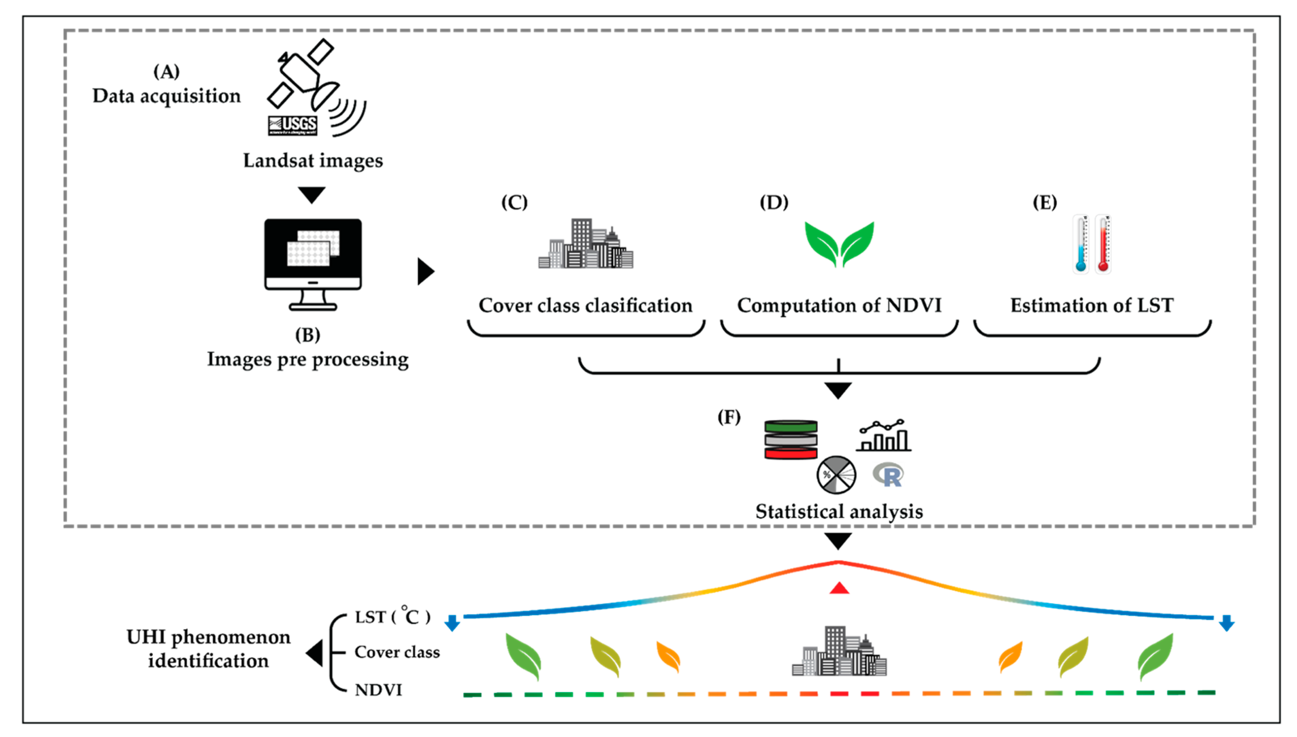
2. Materials and Methods

2.1. Study Area

The study was carried out in a mosaic of different uses and land covers 1,051,011.4 ha of human impacted landscape, located in the municipalities of Mérida, Conkal, and Kanasin, Mexico (coordinates: 21°11’18.42" N; 89°43’17.76" W and 20°41’50.02" N; 89°39’8.02" W) (Figure 1). The region is characterized by a calcareous platform, with karstic soils of biogenic origin, and absence of major topographic features, as well as surface rivers [39]. The combination of geomorphological, climatic, hydrological, soil, and ecological elements of the region encourages a particular development of biodiversity. The climate of the city of Mérida is the driest of subhumid climates with summer rains Ax’(w)w, a high percentage of winter rains and intraannual drought [40]. It is also a region prone to tropical cyclones during the rainy season, and cold fronts during the winter months due to its proximity to the sea and the effects of an ocean current from the Yucatán Channel [41,42]. Two climatic seasons were identified to this study, dry season (March–May) and wet season (July to February); the study area is the driest in the Yucatán Peninsula with an average annual rainfall of 500 mm [43,44]. According to the classification of Miranda and Hernandez-X [45], the dominant vegetation type is tropical dry forest. However, anthropogenic activities such as cattle raising, agriculture, open-pit mining, and the growth of the urban patch modified the vegetation matrix of the tropical dry forest towards secondary succession with different ages of abandonment [46].

2.2. Data Acquisition and Image Preprocessing

The effect of the loss of vegetation cover on the land surface temperature (LST), as a consequence of the increase in urban infrastructure, was evaluated based on a historical analysis of land-cover changes in the municipalities of Conkal, Kanasin, and Mérida. Images were acquired from Landsat-5(MSS/TM), Landsat-7 (ETM+) and Landsat-8 (OLI/TIRS) sensors (USGS; http://www.usgs.gov/ accessed on 2 June 2020) for a period of 24 years (1995, 2000–2001, 2014–2016, and 2018–2019). The analyses were carried out for dry season (February–May) and wet season (November–January) (Table 1). The spectral and spatial resolution of the images varied between the sensors; Landsat TM and ETM+ have seven bands with the same spatial resolution (30 m) and a thermal band of 100 and 60 m, respectively; while Landsat 8 has nine bands at 30 m resolution (OLI), one thermal band at 100 m spatial resolution (TIRS), and one panchromatic band at 15 m (Table 2). Particularly, the following bands were used for the LST calculation: for the Landsat 5 sensor, band 6 was used; while for Landsat 7, band 6_VCID_1 was utilized, here we named as band 6. This last band is recommended for tropical studies because it does not present radiometric saturation in the hottest areas [47]. For Landsat 8, we selected band 10 instead of band 11 to calculate land surface temperature. This is because band 10 has the best adjustment in terms of temperature calculation, while band 11 presents an overestimation [48]. Based on the suggestions of Chuvieco [49], the acquired images were radiometrically and atmospherically corrected to reduce the effect of atmospheric scattering using Semi-Automatic Classification Plugin (SCP) Version 7.0.11-Metera [50], in QGIS Version 3.12 “București” software [51]. This software is an open-source geographic information system for all operative systems. Both QGIS and SCP are widely used for the study of the Earth, supported by remote sensing [52,53,54,55,56]. The general schematic workflow for this study is shown in Figure 2.

2.3. Calculation of Land-Cover Changes

To detect land-cover changes, a supervised classification was performed using the dzetsaka classification tool plugin, with Gaussian Mixture Model [57], with corrected Landsat images for the years 1995, 2000–2001, 2014–2016, and 2018–2019. The years were selected based on two criteria: (1) the end of the 1990s represented an important point in the “modernization” of the state of Yucatán, and Mérida began to have relevance at the national level; (2) the availability of satellite images. The regions of interest (ROI) for each of the classifications were made based on our experience in the area of study and vector information from the National Institute of Statistics and Geography of Mexico [58], as well as with the support of the Google Earth tool. We determined 100 ROI per type of coverage, giving a total of 300 ROI per year. The types of coverage defined were as follows: urban (e.g., houses, buildings, roads, and avenues), vegetation, and bare soil with dispersed vegetation (thereafter, scattered vegetation). Subsequently, the thematic accuracy of each of the classifications was assessed using overall precision, and the accuracy of the classifications was calculated using the Kappa index [59] based on an independent subset of 30 ROI per cover class. A 3-pixel by 3-pixel filter was applied to remove the salt-and-pepper effect from the monitored ratings. Changes of class covers were calculated through a confusion matrix.

2.4. Computation of Normalized Differences Vegetation Index (NDVI) and Land Surface Temperature (LST)

NDVI was calculated following the general normalized difference between band TM4 (near infrared—NIR) and band TM3 (visible red—RED) from the Landsat preprocessed images Equation (1). NDVI is a key element to calculating, afterward, the proportion of the vegetation (PV) and emissivity (ε) necessary to calculated LST.
N D V I = ( N I R R E D ) ( N I R + R E D )
LST calculation is a key component for understanding energy transfer models between the soil–vegetation and the atmosphere [60]. In accordance with the methodology proposed by Avdan and Jovanovska [61] to estimate LST, we used data of the thermal infrared region of each sensor through Semi-Automatic Classification Plugin Version 7.0.11-Metera [50], in the free and open-source software QGIS Version 3.12 “București” [51] (Table 1). First, the spectral radiance () of the top of the atmosphere (TOA) was calculated by introducing band 10 and equations taken from the USGS [62]:
L λ = M L Q c a l + A L O i
where ML represents a multiplicative rescaling factor of the specific band, Qcal is the value of the thermal band image, AL is the rescaling specific factor of the band, and Oi is the correction of the thermal band. The next step was to calculate the brightness temperature (BT) from the absolute radiance values.
B T = ( K 2 ln ( K 1 T O A ) + 1 ) 273.15
where K1 and K2 represent the band-specific thermal conversion constants from metadata. Furthermore, the results were converted from Kelvin to Celsius degrees, adding the absolute zero. In addition, the proportion of vegetation in each pixel was calculated, expressed as Pv from NDVI, according to Equation (4); from this, the land surface emissivity was calculated (Equation (5)). Finally, the real LST was estimated according to Equation (6) [61,63].
P V = [ ( N D V I N D V I m i n ) ] / [ ( N D V I m a x N D V I m i n ) ] 2
ε = 0.004 P V   + 0.986
where 0.004 corresponds to the average emissivities value of bare soil, 0.986 the average emissivity values of the vegetated areas, and Pv is the proportion of vegetation [63].
L S T = [ B T / ( 1 + λ B T ϱ ln ( ε ) ) ]
where BT = brightness temperature; λ = wavelength of the radiance emitted in each band; ρ = constant of Boltzmann (1.38·10–23 J/K), and ε = surface emissivity) [61].

2.5. Statistical Analysis

To determine the influence of the change in coverage on the LST, the years 1995 and 2019 were selected. The LST of the vegetation cover class of the year 1995 was used to compare with the LST of all those pixels that changed cover in 2019; the analysis was carried out using the Student’s t-test. Furthermore, to determine if there were statistically significant differences in the mean of the LST between the cover classes, an analysis of the unidirectional variance (ANOVA) by season was performed. The dependent variables were formally tested for normality and homoscedasticity, while the response variables were transformed as needed with 1/x, log10(x), log10(x + 1), and sqrt(x) to meet linearity assumptions. Finally, to establish the relationship between the LST and the NDVI, the values of temperature and the NDVI were extracted for each of the coverage classes. Subsequently, a regression analysis with cross-validation by station was carried out, and the adjustment was compared using the coefficient of determination (R2). All analyses were performed with the glm2 package [64] in the R [65] software. The general schematic workflow for this study is shown in Figure 2.

3. Results

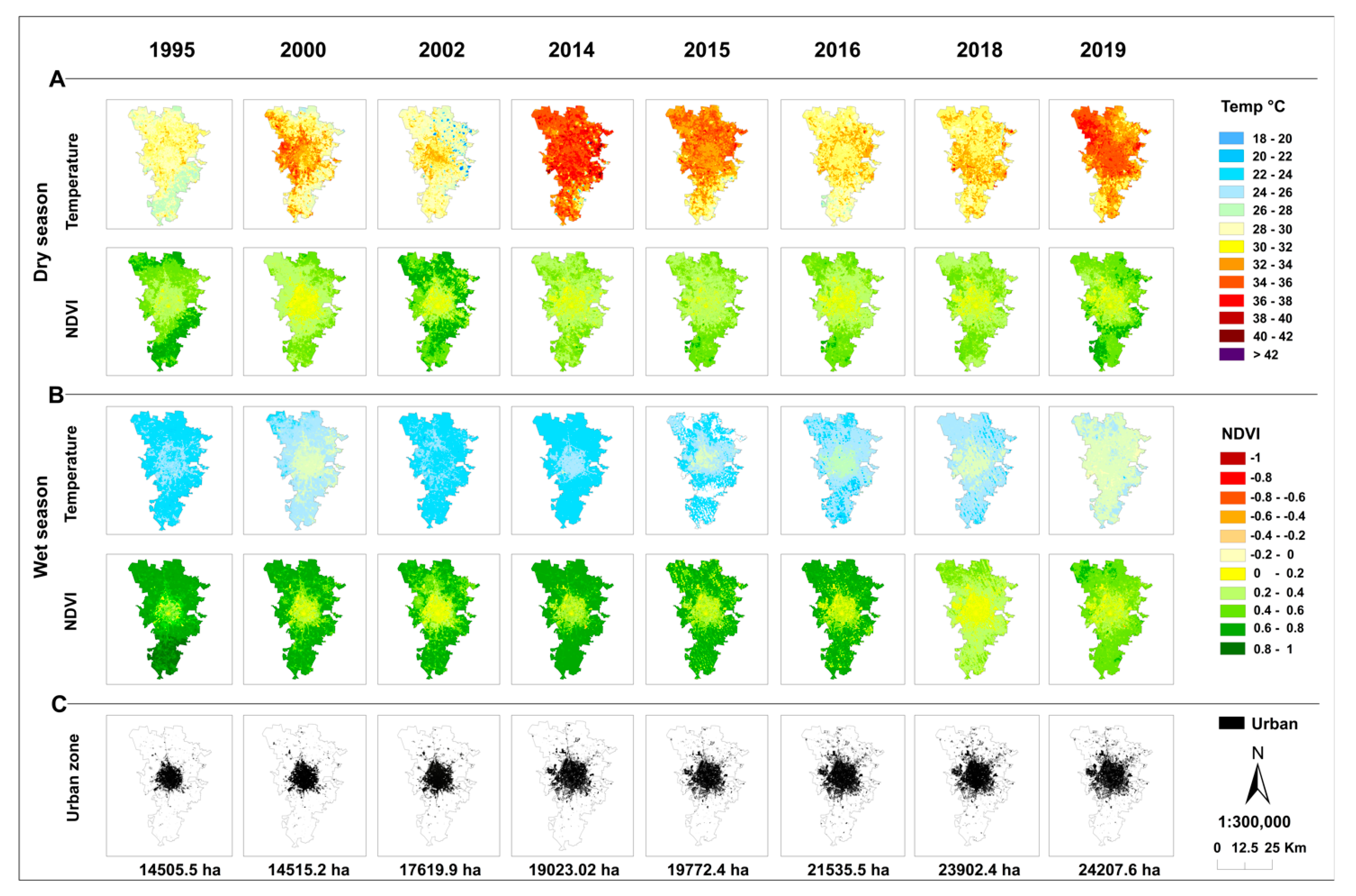
3.1. Land-Cover Changes of Mérida

The total analyzed area was 105,008.3 ha; between 1995 and 2019, 31,679 ha of landscape (30%) changed to another cover class, while 73,209 ha (70%) remained unchanged (Table 3). The urban class registered the greatest increase from 14,505 to 24,215 ha, followed by the scattered vegetation class, which showed an increase from 18,151 ha to 24,225. In contrast, the areas of vigorous vegetation showed a negative trend, as they went from 72,343 to 56,448 ha. The same classification method was carried out in all the Landsat images, and Table 4 shows the overall accuracy (OA), Kappa coefficient, and highest accuracy per cover class per year.

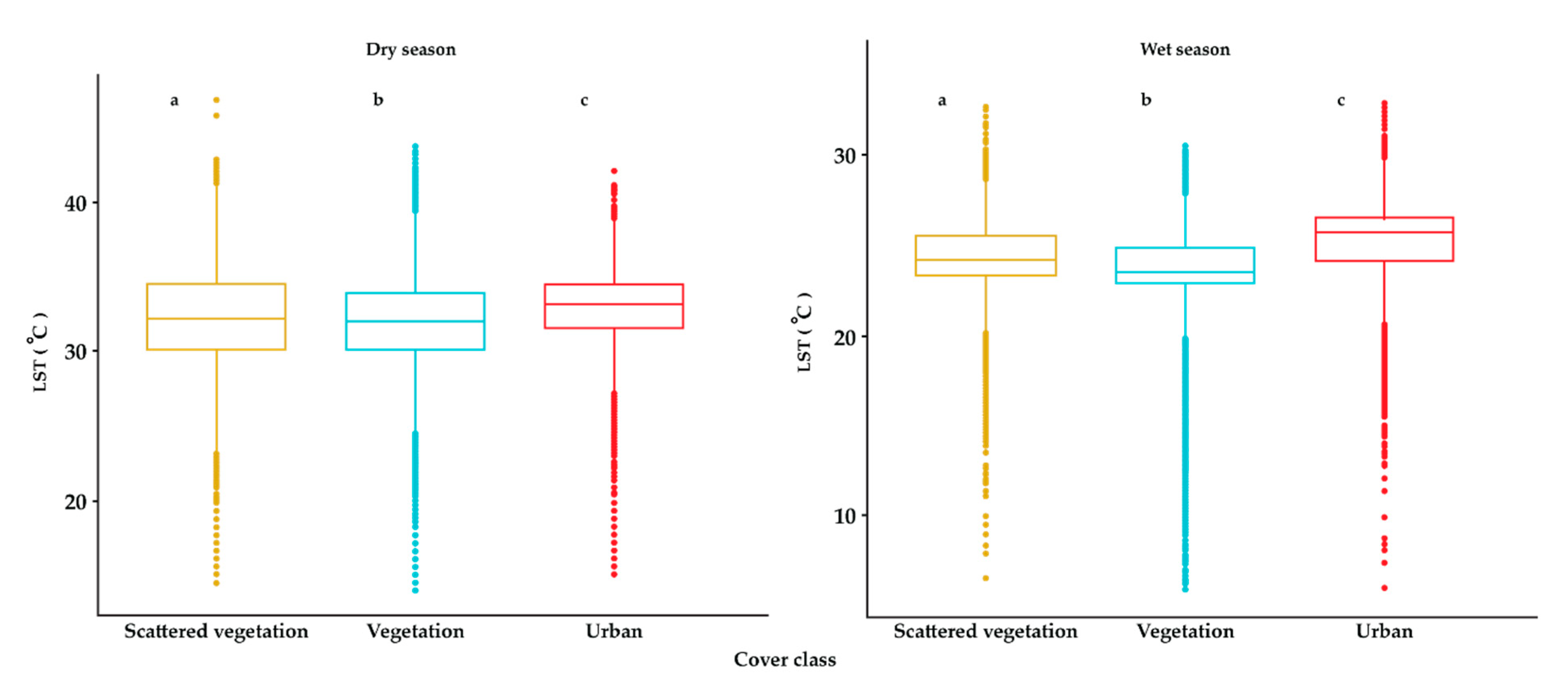
3.2. Historical LST Results

Figure 3A shows the historical spatial distribution of LST in Mérida, calculated from the Landsat images from 1995 to 2019 by dry and wet seasons. In general, an increase in the LST was observed from 1995 to 2019 in both seasons; however, the increase is more evident in the wet season with an increase of approximately 2 to 3 °C. Particularly, in the dry season, the highest temperatures were observed in 2014 and 2019 with an average of LST of 32.90 °C (18.3–47.5 °C) and 35.45 (23.1–47.8 °C), respectively. In the wet season, the year 2000 showed the highest average of LST with 28.25 °C (16–40.5 °C) (Table 5). The LST values showed significant differences between the coverage classes for dry and wet seasons (F = 8532, p = 0.0001; F = 50,636, p = 0.0001, respectively). In the dry season, a greater variation in the LST was observed in the scattered vegetation and vegetation cover classes, contrary to what was observed in the wet season. All classes showed an increase between approximately 8 and 10 °C between dry and wet season (Figure 4).

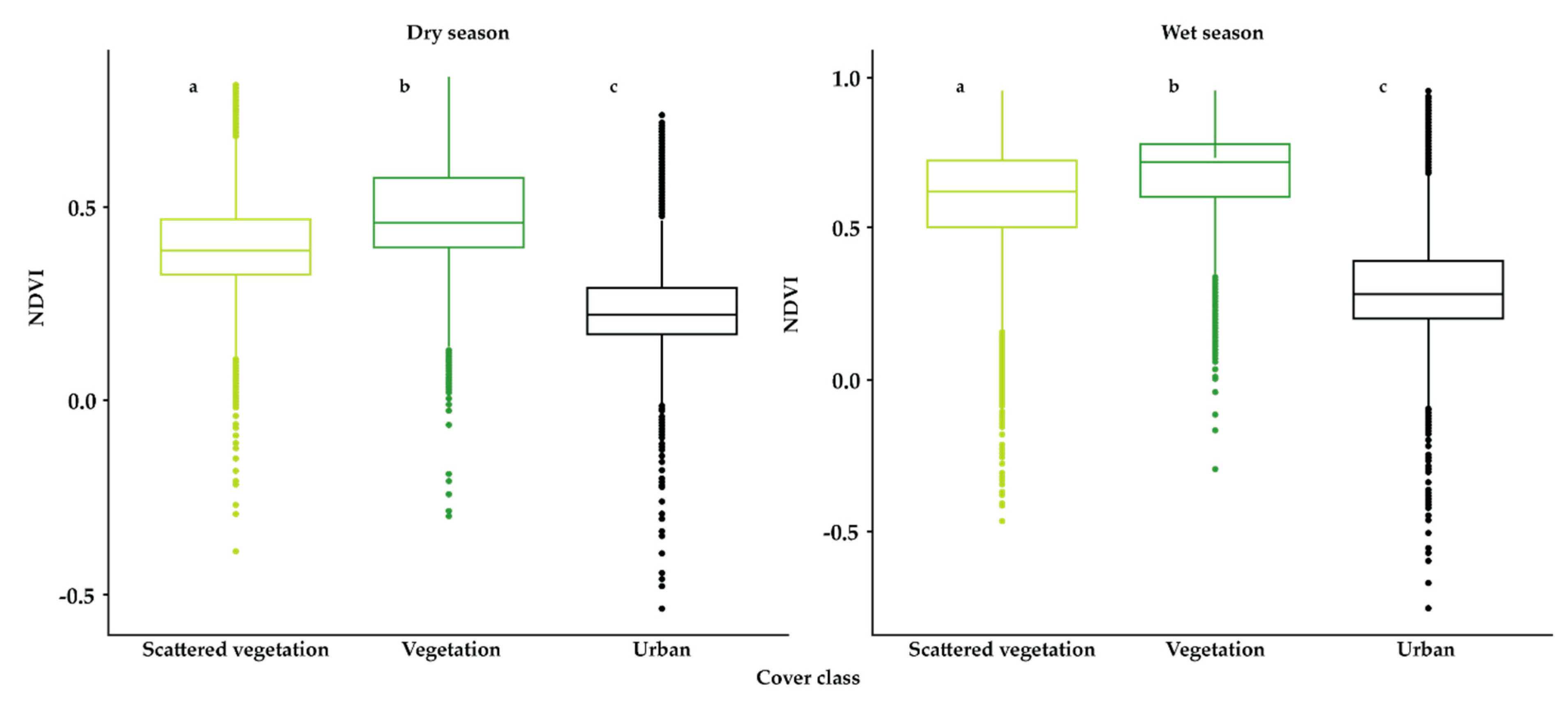
3.3. Historical NDVI Results

Figure 3B shows historical spatial distribution of NDVI values in Mérida. In general, a decreasing pattern in NDVI values is observed in the last 24 years, suggesting a decrease in vegetation vigor, as well as a consequence of the change in land use. In particular, it was observed that the lowest NDVI values are located in the area corresponding to the center of the city, as opposed to the periphery of the study area, where the highest values are located. The variation of the NDVI values in the whole study area is between –0.3 and 0.93 in the dry season and between –0.2 and 0.93 in the wet season. Table 5 shows the median, as well as the maximum and minimum values of the NDVI, and LST per season per year. In terms of coverage classes, significant differences were observed between them (Figure 5). Statistically significant differences were observed in the NDVI values with respect to the coverage classes in the dry season (F = 268,025, p = 0.0001), as well as in the wet season (F = 395,166, p = 0.0001) (Figure 5).

3.4. Relationship between LST, Land Use Change (LUC), and NDVI

Significant differences were found in the mean LST between 1995 (29.36 °C) and 2019 (33.89 °C) (t, 201,651 = 677.02, p = 0.0001), for both the dry and rainy seasons (29.36 °C and 33.89 °C, respectively; (t, 211,288 = 1041.3, p = 0.0001) reported for the city of Mérida, Yucatán. Furthermore, statistically significant differences were found in the mean LST in those pixels that went from vegetation cover class in 1995 to urban in 2019 for dry (t, 20,245 = 6.99, p = 0.0001) and for northern (t, 16,294 = 41.42, p = 0.0001). Regression analysis showed a positive relationship between LST and NDVI using 80% of the data for training and 20% for validation. The model that presented the best fit for estimating the LST from the NDVI was that of the dry season with an R2 = 0.2511 (RMSE = 2.32 °C); while for the northern season the fit was slightly lower, R2 = 0.1476 (RMSE = 1.57 °C).

4. Discussion

Mérida City is historically recognized as a high cultural value city due to its link with the Mayan civilization. In recent years it has received several recognitions as one of the cities with the best quality of life in the world. Consequently, the real estate supply has intensified in the last decade, being one of the most profitable and productive economic sectors at the regional and national level [66,67,68].
Since its foundation (1953), Mérida had a configuration that favored green and treed areas; however, in the last 10 years it has experienced accelerated horizontal growth [66] towards the periphery, mainly in the eastern and western zones, under a construction model that bets on a spatial arrangement that seeks to increase the number of homes, sacrificing green spaces [67,68].
The main consequences of urban growth are the imminent loss or degradation of natural vegetation cover. In the case of Mérida, the horizontal growth of the city has implied the absorption of small settlements, transformation of areas with scattered vegetation, and reduction of the natural vegetation cover of 15,895 ha in the last 24 years. According to Sullivan and Ward [69], this type of growth in urban areas causes significant loss of green areas, agricultural land, in addition to increased levels of consumerism and larger traveling distances in people’s daily lives [67,70].
NDVI values obtained suggest a global decrease in vegetation vigor in the region, as a consequence of the land use change in the last 24 years. Particularly for Mérida and its metropolitan area, the NDVI values estimated are between 0.2–0.5. Furthermore, the values observed within the city suggest that the current vegetation is not vigorous enough to maintain ecosystem services and that the observed mix between urban areas and vegetation suggests areas of environmental stress caused by edge effects. Regarding the vegetation outside the urban zone, different density and coverage conditions were observed (NDVI: 0.6–1) in a clear gradient of vegetation degradation that decreases with distance to the urban zone, similar to an edge effect. Finally, the correlation observed between cover classes and NDVI values in this study is in agreement with that found by Ferreira and Duarte [71] in shrub and bush species, suggesting that most of the vegetation is deciduous [46].
Degradation, or loss of vegetation, alter the balance of solar radiation that falls on the Earth’s surface, that modifies the distribution of humidity and heat in the atmosphere, resulting in a local increase in temperature [5,71,72]. For the study area, in the last two decades, 15,895 ha of natural vegetation have been lost; 9710 ha of these have been replaced by artificial materials, such as concrete, cement, or pavement, with a significant impact on the modification of the local temperature [68].
The results show that the highest temperatures are focused into the Mérida urban zone, and they have increased over time, contrary to what was observed in peripheral areas that maintain vegetation cover. These results suggests that climate change processes occur at different spatial scales. At local scales, the increase in urban infrastructure increases albedo, decreases evapotranspiration, and generates the UHI phenomenon [5,71,72], while at regional scale, forest cover keeps the temperature relatively constant, and the climatic variations could be associated with regional or global climatic events or phenomena (El Niño and the Southern Oscillation, or global climate change [73,74,75]). This is similar to other tropical cities as Beijing, Changchun, and Hangzhou, China [1,8,11], Cameron Highlands, Malaysia [76], or Shiraz, Iran [77]. In all cases, UHI phenomena are associated with the extension of the urban area, type of structures and material, density housing, and presence of areas with continuous vegetation within the city.
In the case of Mérida, the difference in LST between urban areas and the peripheral areas with vegetation (scattered or dense) is on average 3.5 °C at the beginning and end of the study season, and is maintained in both seasons, similar to that observed by Adeyeri et al. [78], Ferreira and Duarte [71], and Dang et al. [79], among other authors.
Particularly in the urban zone, high temperatures were observed in the periphery (east and west) of the city, this is associated with concrete, pavement surfaces, and bare soil on the city’s edge. In contrast, the north of the city, where residential houses and greater treed areas are, presents a cooler condition, in accordance with that reported by Pérez-Medina and López-Falfán [68] for the study area, and by Ferreira and Duarte [71], Martín-Vide and Moreno-García [7], and Wang et al. [80], among others, for similar studies.
Likewise, specific sites with extreme temperatures were identified, associated with the cement industry, the sanitary landfill, fires, and burned areas as part of agricultural activities, in the same way it was observed that, in recent years, the temperature between these hot spots and the rest of city is increasingly similar, which shows the occurrence of the UHI. In big cities where the UHI phenomenon has been recorded, the heat island is concentrated in the center of the cities [22,24,78,79,81]. However, for Mérida’s urban zone, the heat island is not located in the center, but in the periphery, where the new developments are located, as pointed out by Pérez-Medina and López-Falfán [68]. With regard to the lower temperatures, they are distributed on the city outskirts, in areas with the presence of water (artificial lakes) and areas with dense, natural, or permanently irrigated vegetation, such as agricultural fields or the golf club.
The obtained results confirm the importance of green and treed areas, natural or artificial, to help reduce the temperature of the surface and the air [46,78], an issue of great relevance for a region with dry subhumid climate, such as Mérida [40], where the average annual temperature is 46 °C in the dry season, and 34 °C in the wet season.
In dry tropical cities such as Mérida, the climatic conditions accentuate the perception of the UHI effect, which reduces the comfort level of the inhabitants, increases the dependence on cooling, favors the presence of pollutants and health problems, among other effects [5,68]. In cities with projections of rapid expansion and extreme hot weather, such as Mérida, it is critical to consider, in the planning of new housing developments, an adequate distribution and density of vegetation as well as promoting the creation of green spaces within the current settlements, to mitigate and prevent the UHI phenomenon [26,82,83], among countless other environmental, social, and economic benefits [8,67,68].

5. Conclusions

The recognition of Mérida as one of the cities with the best quality of life in the world has been a driving force behind the demand for residential spaces in recent decades. The degradation and loss of vegetation in Mérida City and its surroundings has led to the modification of the microclimate, accentuating the high temperatures in the region within the urban area.
The extensive areas with vegetation, natural or irrigated, inside and outside the city, contribute to mitigating the warm natural temperatures in this dry tropical city, mainly in the dry season. The hotspot identification highlights the need to promote the conservation of areas with natural vegetation, and to integrate green spaces in the planning of new housing developments, to mitigate the UHI phenomenon, reduce energy consumption and greenhouse gas emissions, raise the comfort level of the inhabitants, and contribute to the sustainability of the city.

Author Contributions

Erika Betzabeth Palafox-Juárez and Jorge Omar López-Martínez conceived and designed the experiments, analyzed the data, prepared figures and tables, wrote drafts of the paper, and approved the final draft; José Luis Hernández-Stefanoni reviewed and edited the manuscript; Héctor Hernández-Nuñez performed data curation and spatial analysis. All authors have read and agreed to the published version of the manuscript.

Funding

This research was funded by CONACyT (Consejo Nacional de Ciencia y Tecnología)—Proyecto No. 526 Manejo de datos obtenidos por la Estación para la Recepción de Información Satelital ERIS-Chetumal.

Institutional Review Board Statement

Not applicable, this study not involving humans or animals.

Informed Consent Statement

Not applicable, this study not involving humans or animals.

Data Availability Statement

To access the data please contact the authors.

Acknowledgments

United States Geological Survey (USGS) website (https://earthexplorer.usgs.gov/ accessed on 2 June 2020) for providing the Landsat TM, Landsat ETM+, and Landsat OLI TIRS images used, and M.C. Dinosca Rondón Rivera for their invaluable technical support.

Conflicts of Interest

The authors declare no conflict of interest.

References

  1. Yang, C.; He, X.; Yan, F.; Yu, L.; Bu, K.; Yang, J.; Chang, L.; Zhang, S. Mapping the Influence of Land Use/Land Cover Changes on the Urban Heat Island Effect—A Case Study of Changchun, China. Sustain. Sci. Pract. Policy 2017, 9, 312. [Google Scholar] [CrossRef] [Green Version]
  2. Glaeser, E.L. A World of Cities: The Causes and Consequences of Urbanization in Poorer Countries. J. Eur. Econ. Assoc. 2014, 12, 1154–1199. [Google Scholar] [CrossRef]
  3. Wup, U.N. World Urbanization Prospects: The 2018 Revision (ST/ESA/SER. A/420); United Nations, Department of Economic and Social Affairs, Population Division: New York, NY, USA, 2019. [Google Scholar]
  4. Instituto Nacional de Estadística y Geografía (INEGI). Censo de Población y Vivienda. 2010. Resultados definitivos, México. 2011. Available online: https://www.inegi.org.mx/programas/ccpv/2010/ (accessed on 12 October 2020).
  5. Ciardini, V.; Caporaso, L.; Sozzi, R.; Petenko, I.; Bolignano, A.; Morelli, M.; Melas, D.; Argentini, S. Interconnections of the urban heat island with the spatial and temporal micrometeorological variability in Rome. Urban. Clim. 2019, 29, 100493. [Google Scholar] [CrossRef]
  6. Romero Rodríguez, L.; Sánchez Ramos, J.; Sánchez de la Flor, F.J.; Álvarez Domínguez, S. Analyzing the urban heat Island: Comprehensive methodology for data gathering and optimal design of mobile transects. Sustain. Cities Soc. 2020, 55, 102027. [Google Scholar] [CrossRef]
  7. Martin-Vide, J.; Moreno-Garcia, M.C. Probability values for the intensity of Barcelona’s urban heat island (Spain). Atmos. Res. 2020, 240, 104877. [Google Scholar] [CrossRef]
  8. Hou, H.; Estoque, R.C. Detecting Cooling Effect of Landscape from Composition and Configuration: An Urban Heat Island Study on Hangzhou. Urban. For. Urban. Green. 2020, 53, 126719. [Google Scholar] [CrossRef]
  9. Kim, H.H. Urban heat island. Int. J. Remote Sens. 1992, 13, 2319–2336. [Google Scholar] [CrossRef]
  10. Chen, X.-L.; Zhao, H.-M.; Li, P.-X.; Yin, Z.-Y. Remote sensing image-based analysis of the relationship between urban heat island and land use/cover changes. Remote Sens. Environ. 2006, 104, 133–146. [Google Scholar] [CrossRef]
  11. Zhao, X.; Yang, S.; Shen, S.; Hai, Y.; Fang, Y. Analyzing the relationship between urban heat island and land use/cover changes in Beijing using remote sensing images. Remote Sens. Modeling Ecosyst. Sustain. VI 2009, 7454, 74541J. [Google Scholar]
  12. Aslan, N.; Koc-San, D. Analysis of relationship between urban heat island effect and land use/cover type using landsat 7 etm and landsat 8 oli images. ISPRS Int. Arch. Photogramm. Remote Sens. Spat. Inf. Sci. 2016, XLI-B8, 821–828. [Google Scholar] [CrossRef]
  13. Tam, B.Y.; Gough, W.A.; Mohsin, T. The impact of urbanization and the urban heat island effect on day to day temperature variation. Urban. Clim. 2015, 12, 1–10. [Google Scholar] [CrossRef]
  14. Soltani, A.; Sharifi, E. Daily variation of urban heat island effect and its correlations to urban greenery: A case study of Adelaide. Front. Archit. Res. 2017, 6, 529–538. [Google Scholar] [CrossRef]
  15. Keeling, C.D.; Whorf, T.P.; Wahlen, M.; van der Plichtt, J. Interannual extremes in the rate of rise of atmospheric carbon dioxide since 1980. Nature 1995, 375, 666–670. [Google Scholar] [CrossRef]
  16. Peñuelas, J.; Rutishauser, T.; Filella, I. Ecology. Phenology feedbacks on climate change. Science 2009, 324, 887–888. [Google Scholar] [CrossRef] [Green Version]
  17. Richardson, A.D.; Keenan, T.F.; Migliavacca, M.; Ryu, Y.; Sonnentag, O.; Toomey, M. Climate change, phenology, and phenological control of vegetation feedbacks to the climate system. Agric. For. Meteorol. 2013, 169, 156–173. [Google Scholar] [CrossRef]
  18. Villarreal, S.; Vargas, R.; Yepez, E.A.; Acosta, J.S.; Castro, A.; Escoto-Rodriguez, M.; Lopez, E.; Martínez-Osuna, J.; Rodriguez, J.C.; Smith, S.V.; et al. Contrasting precipitation seasonality influences evapotranspiration dynamics in water-limited shrublands: Shrubland evapotranspiration dynamics. J. Geophys. Res. Biogeosci. 2016, 121, 494–508. [Google Scholar] [CrossRef] [Green Version]
  19. Dong, S.X.; Davies, S.J.; Ashton, P.S.; Bunyavejchewin, S.; Supardi, M.N.N.; Kassim, A.R.; Tan, S.; Moorcroft, P.R. Variability in solar radiation and temperature explains observed patterns and trends in tree growth rates across four tropical forests. Proc. Biol. Sci. 2012, 279, 3923–3931. [Google Scholar] [CrossRef]
  20. Wright, S.J. Phenological Responses to Seasonality in Tropical Forest Plants. In Tropical Forest Plant Ecophysiology; Mulkey, S.S., Chazdon, R.L., Smith, A.P., Eds.; Springer: Boston, MA, USA, 1996; pp. 440–460. ISBN 9781461311638. [Google Scholar]
  21. Estoque, R.C.; Murayama, Y. Monitoring surface urban heat island formation in a tropical mountain city using Landsat data (1987–2015). ISPRS J. Photogramm. Remote Sens. 2017, 133, 18–29. [Google Scholar] [CrossRef]
  22. De Faria Peres, L.; de Lucena, A.J.; Rotunno Filho, O.C.; de Almeida França, J.R. The urban heat island in Rio de Janeiro, Brazil, in the last 30 years using remote sensing data. Int. J. Appl. Earth Obs. Geoinf. 2018, 64, 104–116. [Google Scholar] [CrossRef]
  23. Voogt, J.A.; Oke, T.R. Thermal remote sensing of urban climates. Remote Sens. Environ. 2003, 86, 370–384. [Google Scholar] [CrossRef]
  24. Zhou, D.; Zhao, S.; Liu, S.; Zhang, L.; Zhu, C. Surface urban heat island in China’s 32 major cities: Spatial patterns and drivers. Remote Sens. Environ. 2014, 152, 51–61. [Google Scholar] [CrossRef]
  25. Chrysoulakis, N. Estimation of the all-wave urban surface radiation balance by use of ASTER multispectral imagery and in situ spatial data. J. Geophys. Res. D Atmos. 2003, 108. [Google Scholar] [CrossRef] [Green Version]
  26. Kato, S.; Yamaguchi, Y. Analysis of urban heat-island effect using ASTER and ETM+ Data: Separation of anthropogenic heat discharge and natural heat radiation from sensible heat flux. Remote Sens. Environ. 2005, 99, 44–54. [Google Scholar] [CrossRef]
  27. Liu, Y.; Hiyama, T.; Yamaguchi, Y. Scaling of land surface temperature using satellite data: A case examination on ASTER and MODIS products over a heterogeneous terrain area. Remote Sens. Environ. 2006, 105, 115–128. [Google Scholar] [CrossRef]
  28. Zhou, W.; Huang, G.; Cadenasso, M.L. Does spatial configuration matter? Understanding the effects of land cover pattern on land surface temperature in urban landscapes. Landsc. Urban. Plan. 2011, 102, 54–63. [Google Scholar] [CrossRef]
  29. Wang, Y.; Akbari, H. Urban heat island and mitigation solutions evaluation in cold climates: A case of Montreal. Adv. Environ. Res. 2017, 54, 143–177. [Google Scholar]
  30. Yuan, F.; Bauer, M.E. Comparison of impervious surface area and normalized difference vegetation index as indicators of surface urban heat island effects in Landsat imagery. Remote Sens. Environ. 2007, 106, 375–386. [Google Scholar] [CrossRef]
  31. Sheng, L.; Tang, X.; You, H.; Gu, Q.; Hu, H. Comparison of the urban heat island intensity quantified by using air temperature and Landsat land surface temperature in Hangzhou, China. Ecol. Indic. 2017, 72, 738–746. [Google Scholar] [CrossRef]
  32. Imhoff, M.L.; Zhang, P.; Wolfe, R.E.; Bounoua, L. Remote sensing of the urban heat island effect across biomes in the continental USA. Remote Sens. Environ. 2010, 114, 504–513. [Google Scholar] [CrossRef] [Green Version]
  33. Huete, A.; Didan, K.; Miura, T.; Rodriguez, E.P.; Gao, X.; Ferreira, L.G. Overview of the radiometric and biophysical performance of the MODIS vegetation indices. Remote Sens. Environ. 2002, 83, 195–213. [Google Scholar] [CrossRef]
  34. Olofsson, P.; Eklundh, L. Estimation of absorbed PAR across Scandinavia from satellite measurements. Part II: Modeling and evaluating the fractional absorption. Remote Sens. Environ. 2007, 110, 240–251. [Google Scholar] [CrossRef]
  35. Pirotti, F.; Parraga, M.A.; Stuaro, E.; Dubbini, M.; Masiero, A.; Ramanzin, M. NDVI From landsat 8 vegetation indices to study movement dynamics of Capra ibex in mountain areas. Int. Arch. Photogramm. Remote Sens. Spat. Inf. Sci. 2014. [Google Scholar] [CrossRef] [Green Version]
  36. Ridd, M.K. Exploring a VIS (vegetation-impervious surface-soil) model for urban ecosystem analysis through remote sensing: Comparative anatomy for cities. Int. J. Remote Sens. 1995, 16, 2165–2185. [Google Scholar] [CrossRef]
  37. Carlson, T.N.; Traci Arthur, S. The impact of land use—land cover changes due to urbanization on surface microclimate and hydrology: A satellite perspective. Glob. Planet. Chang. 2000, 25, 49–65. [Google Scholar] [CrossRef]
  38. Deng, Y.; Wang, S.; Bai, X.; Tian, Y.; Wu, L.; Xiao, J.; Chen, F.; Qian, Q. Relationship among land surface temperature and LUCC, NDVI in typical karst area. Sci. Rep. 2018, 8, 641. [Google Scholar] [CrossRef] [PubMed]
  39. Hubp, J.L.; Quesado, J.F.A.; Pereño, R.E. Rasgos geomorfológicos mayores de la Península de Yucatán. Revista Mexicana de Ciencias Geológicas 1992, 10, 143–150. [Google Scholar]
  40. García Amaro, E. Modificaciones al Sistema de Clasificación Climática de Köppen; Universidad Nacional Autónoma de México: Mexico City, Mexico, 2004. [Google Scholar]
  41. Orellana, R.; Islebe, G.; Espadas, C. Presente, pasado y futuro de los climas de la Península de Yucatán. In Naturaleza y Sociedad del Área maya. Pasado Presente y Futuro; Colunga García, P., Marín, A., Saavedra, L., Eds.; Academia Mexicana de Ciencias y Centro de Investigación Científica de Yucatán: Mérida, México, 2003; pp. 37–52. [Google Scholar]
  42. Orellana, R.; Espadas, C.; Conde, C.; Gay, C. Atlas escenarios de cambio climático en la Península de Yucatán. Mérida: Centro de Investigación Científica de Yucatán (CICY) 2009, 43, 191–193. [Google Scholar]
  43. Capurro, L.; Euán, J.; Herrera, J. Manejo sustentable del ecosistema costero de Yucatán. Avance y Perspectiva 2002, 21, 195–204. [Google Scholar]
  44. Torrescano-Valle, N.; Folan, W.J. Physical Settings, Environmental History with an Outlook on Global Change. In Biodiversity and Conservation of the Yucatán Peninsula; Islebe, G.A., Calmé, S., León-Cortés, J.L., Schmook, B., Eds.; Springer International Publishing: Cham, Switzerland, 2015; pp. 9–37. ISBN 9783319065298. [Google Scholar]
  45. Miranda, F.; Hernández-X, E. Los tipos de vegetación de México y su clasificación. Bot. Sci. 1963, 29–179. [Google Scholar] [CrossRef]
  46. Islebe, G.A.; Sánchez-Sánchez, O.; Valdéz-Hernández, M.; Weissenberger, H. Distribution of Vegetation Types. In Biodiversity and Conservation of the Yucatán Peninsula; Islebe, G.A., Calmé, S., León-Cortés, J.L., Schmook, B., Eds.; Springer International Publishing: Cham, Switzerland, 2015; pp. 39–53. ISBN 9783319065298. [Google Scholar]
  47. Irish, R.R.; NASA. Landsat 7 Science Data Users Handbook. 2000; pp. 415–430. Available online: https://www.usgs.gov/core-science-systems/nli/landsat/landsat-7-data-users-handbook (accessed on 2 June 2020).
  48. Ihlen, V. Landsat 8 (L8) Data Users Handbook. U.S. Geological Survey. 2019. Available online: https://www.usgs.gov/core-science-systems/nli/landsat/landsat-8-data-users-handbook (accessed on 2 June 2020).
  49. Chuvieco, E. Fundamentals of Satellite Remote Sensing; CRC Press: Boca Raton, FL, USA, 2009; ISBN 9781420021516. [Google Scholar]
  50. Congedo, L. Semi-Automatic Classification Plugin User Manual. Tech. Rep. Navtradevcen 2016. [Google Scholar] [CrossRef]
  51. QGIS. Available online: https://qgis.org/en/site (accessed on 15 May 2020).
  52. Leroux, L.; Congedo, L.; Bellón, B.; Gaetano, R.; Bégué, A. Land cover mapping using Sentinel-2 images and the semi-automatic classification plugin: A Northern Burkina Faso case study. QGIS Appl. Agric. For. 2018, 2, 119–151. [Google Scholar]
  53. Pereira, L.F.; Guimarães, R.M.F. Mapping land uses/covers with Semi-automatic Classification Plugin: Which data set, classifier and sampling design? Nativa Pesquisas Agrárias e 2019, 7, 70–76. [Google Scholar] [CrossRef]
  54. Balaji, K.; Kamarapermual, R.; Ragunath, K.P.; Jagadeeswaran, R. Evaluating Urbanisation by Land Use/Land Cover Change Detection in Coimbatore Using Remote Sensing and Geographic Information System. Int. J. Agric. Sci. ISSN 2020, 12, 9706–9709. [Google Scholar]
  55. Henrico, S.; Coetzee, S.; Cooper, A.; Rautenbach, V. Acceptance of open source geospatial software: Assessing QGIS in South Africa with the UTAUT2 model. Trans. GIS 2020, 1–23. [Google Scholar] [CrossRef]
  56. Yanru, H.; Masoudi, M.; Chadala, A.; Olszewska-Guizzo, A. Visual Quality Assessment of Urban Scenes with the Contemplative Landscape Model: Evidence from a Compact City Downtown Core. Remote Sens. 2020, 12, 3517. [Google Scholar] [CrossRef]
  57. Karasiak, N.; Perbet, P. Remote sensing of distinctive vegetation in Guiana amazonian park. In QGIS and Applications in Agriculture and Forest; John Wiley & Sons, Inc.: Hoboken, NJ, USA, 2018; pp. 215–245. ISBN 9781119457107. [Google Scholar]
  58. Instituto Nacional de Estadística y Geografía (INEGI). Conjunto de Datos Vectoriales de uso del Suelo y Vegetación Escala 1: 250 000; Serie VI (Conjunto Nacional). 2017. Available online: https://www.inegi.org.mx/temas/usosuelo/ (accessed on 25 August 2020).
  59. Green, E.; Mumby, P.; Edwards, A.; Clark, C. Remote Sensing: Handbook for Tropical Coastal Management; United Nations Educational, Scientific and Cultural Organization (UNESCO): Paris, France, 2000. [Google Scholar]
  60. Vlassova, L.; Perez-Cabello, F.; Nieto, H.; Martín, P.; Riaño, D.; De la Riva, J. Assessment of Methods for Land Surface Temperature Retrieval from Landsat-5 TM Images Applicable to Multiscale Tree-Grass Ecosystem Modeling. Remote Sens. 2014, 6, 4345–4368. [Google Scholar] [CrossRef] [Green Version]
  61. Avdan, U.; Jovanovska, G. Algorithm for Automated Mapping of Land Surface Temperature Using LANDSAT 8 Satellite Data. J. Sens. 2016, 1480307. [Google Scholar] [CrossRef] [Green Version]
  62. Chander, G.; Markham, B.L.; Helder, D.L. Summary of current radiometric calibration coefficients for Landsat MSS, TM, ETM+, and EO-1 ALI sensors. Remote Sens. Environ. 2009, 113, 893–903. [Google Scholar] [CrossRef]
  63. Sobrino, J.A.; Raissouni, N. Toward remote sensing methods for land cover dynamic monitoring: Application to Morocco. Int. J. Remote Sens. 2000, 21, 353–366. [Google Scholar] [CrossRef]
  64. Marschner, I.; Donoghoe, M.W.; Donoghoe, M.M.W. Package “glm2”. J. Vol. 2018, 3, 12–15. [Google Scholar]
  65. Team, R.C. R development core team. RA Lang. Environ. Stat. Comput 2013, 55, 275–286. [Google Scholar]
  66. OECD. Territorial Reviews: Yucatan, Mexico 2007. OECD Territ. Rev. 2007. Available online: https://www.oecd.org/mexico/oecdterritorialreviewsyucatanmexico.htm (accessed on 3 November 2020).
  67. Cerón-Palma, I.; Sanyé-Mengual, E.; Oliver-Solà, J.; Montero, J.-I.; Ponce-Caballero, C.; Rieradevall, J. Towards a green sustainable strategy for social neighbourhoods in Latin America: Case from social housing in Merida, Yucatan, Mexico. Habitat Int. 2013, 38, 47–56. [Google Scholar] [CrossRef]
  68. Pérez-Medina, S.; López-Falfán, I. Áreas verdes y arbolado en Mérida, Yucatán. Hacia una sostenibilidad urbana. Economía Sociedad y Territorio 2015, 15, 01–33. [Google Scholar] [CrossRef] [Green Version]
  69. Sullivan, E.; Ward, P.M. Sustainable housing applications and policies for low-income self-build and housing rehab. Habitat Int. 2012, 36, 312–323. [Google Scholar] [CrossRef]
  70. Turok, I. Deconstructing density: Strategic Dilemmas Confronting the Post-Apartheid city. Cities 2011, 28, 470–477. [Google Scholar] [CrossRef] [Green Version]
  71. Ferreira, L.S.; Duarte, D.H.S. Exploring the relationship between urban form, land surface temperature and vegetation indices in a subtropical megacity. Urban. Clim. 2019, 27, 105–123. [Google Scholar] [CrossRef]
  72. Kitsara, G.; Papaioannou, G.; Retalis, A.; Paronis, D.; Kerkides, P. Estimation of air temperature and reference evapotranspiration using MODIS land surface temperature over Greece. Int. J. Remote Sens. 2018, 39, 924–948. [Google Scholar] [CrossRef]
  73. Fyfe, J.C.; Gillett, N.P.; Zwiers, F.W. Overestimated global warming over the past 20 years. Nat. Clim. Chang. 2013, 3, 767–769. [Google Scholar] [CrossRef]
  74. COMISION NACIONAL DEL AGUA, Resúmenes Mensuales de Temperatura y Lluvias. 2016. Available online: https://smn.conagua.gob.mx/es/climatologia/temperaturas-y-lluvias/resumenes-mensuales-de-temperaturas-y-lluvias (accessed on 12 November 2020).
  75. Seddon, A.W.R.; Macias-Fauria, M.; Long, P.R.; Benz, D.; Willis, K.J. Sensitivity of global terrestrial ecosystems to climate variability. Nature 2016, 531, 229–232. [Google Scholar] [CrossRef] [PubMed] [Green Version]
  76. How Jin Aik, D.; Ismail, M.H.; Muharam, F.M. Land Use/Land Cover Changes and the Relationship with Land Surface Temperature Using Landsat and MODIS Imageries in Cameron Highlands, Malaysia. Land 2020, 9, 372. [Google Scholar] [CrossRef]
  77. Kamali Maskooni, E.; Hashemi, H.; Berndtsson, R.; Daneshkar Arasteh, P.; Kazemi, M. Impact of spatiotemporal land-use and land-cover changes on surface urban heat islands in a semiarid region using Landsat data. Int. J. Digit. Earth 2020, 14, 1–21. [Google Scholar] [CrossRef]
  78. Adeyeri, O.E.; Akinluyi, F.O.; Ishola, K.A. Spatio-temporal trend of vegetation cover over Abuja using Landsat datasets. Int. J. Agric. Environ. Res. 2017, 3. [Google Scholar] [CrossRef]
  79. Dang, T.; Yue, P.; Bachofer, F.; Wang, M.; Zhang, M. Monitoring Land Surface Temperature Change with Landsat Images during Dry Seasons in Bac Binh, Vietnam. Remote Sens. 2020, 12, 4067. [Google Scholar] [CrossRef]
  80. Wang, S.; Ma, Q.; Ding, H.; Liang, H. Detection of urban expansion and land surface temperature change using multi-temporal landsat images. Resour. Conserv. Recycl. 2018, 128, 526–534. [Google Scholar] [CrossRef]
  81. Blake, R.; Grimm, A.; Ichinose, T.; Horton, R.; Gaffin, S.; Jiong, S.; Bader, D.; Cecil, L.D. Urban climate: Processes, trends and projections. In Climate Chagne and Cities: First Assessment Report of the Urban Climate Change Research Newtork; Tosenzweig, C., Solecki, W., Hammer, S., Mehrotra, S., Eds.; Cambridge University Press: Cambridge, UK, 2011; pp. 43–81. [Google Scholar] [CrossRef]
  82. Estes, M.G., Jr. Urban Heat Island Mitigation Strategies. 2000, pp. 1–4. Available online: https://www.researchgate.net/publication/294517225_Urban_heat_island_mitigation_strategies (accessed on 12 November 2020).
  83. Sanchez, L.; Reames, T.G. Cooling Detroit: A socio-spatial analysis of equity in green roofs as an urban heat island mitigation strategy. Urban For. Urban Green. 2019, 44, 126331. [Google Scholar] [CrossRef]
Figure 1. Study area: urban zone of Mérida, Yucatán, Mexico.
Ijgi 10 00076 g001
Figure 2. Graphic workflow of stages to identify urban heat island (UHI) phenomenon: (A) Data acquisition. (B) Imagery pre-procesing, (C) Land cover classification, (D)calculation of NDVI, (E) estimation of and surfer temperature and (F) statistical analysis.
Ijgi 10 00076 g002
Figure 3. Spatiotemporal variation of land surface temperature and NDVI in dry season (A), wet season (B) and urban zone extension (C).
Ijgi 10 00076 g003
Figure 4. Land surfer temperature variation per classes of land cover in the dry season (left) and the wet season (right), different letters show statistically significant differences.
Ijgi 10 00076 g004
Figure 5. NDVI variation for land cover classes in the dry season (left) and the wet season (right), different letters show statistically significant differences.
Ijgi 10 00076 g005
Table 1. List of Landsat images used to carry out the analysis.
IDImage NamePathRowYearMonthDay
Dry Season
1LT05_L1TP_020045_19950423_20170109_01_T120451995423
2LT05_L1TP_020046_19950423_20170108_01_T120461995423
3LE07_L1TP_020045_20000428_20170212_01_T120452000428
4LE07_L1TP_020046_20000428_20170212_01_T120462000428
5LE07_L1TP_020045_20020317_20170131_01_T120452002317
6LE07_L1TP_020046_20020317_20170131_01_T120462002317
7LC08_L1TP_020045_20140427_20170307_01_T120452014427
8LC08_L1TP_020046_20140427_20170307_01_T120462014427
9LC08_L1TP_020045_20150414_20170228_01_T120452015414
10LC08_L1TP_020046_20150414_20170228_01_T120462015414
11LC08_L1TP_020045_20160416_20170326_01_T120452016326
12LC08_L1TP_020046_20160416_20170326_01_T120462016326
13LC08_L1TP_020045_20180406_20180417_01_T12045201846
14LC08_L1TP_020046_20180406_20180417_01_T12046201846
15LC08_L1TP_020045_20190511_20190521_01_T120452019511
16LC08_L1TP_020046_20190511_20190521_01_T120462019511
Wet Season
17LT05_L1TP_020045_19951203_20170105_01_T120451995123
18LT05_L1TP_020046_19951203_20170106_01_T120461995123
19LE07_L1TP_020045_20001106_20170209_01_T120452000116
20LE07_L1TP_020046_20001106_20170209_01_T120462000116
21LE07_L1TP_020045_20021230_20170127_01_T1204520021230
22LE07_L1TP_020046_20021230_20170127_01_T1204620021230
23LC08_L1TP_020045_20140105_20170307_01_T12045201415
24LC08_L1TP_020046_20140105_20170307_01_T12046201415
25LC08_L1TP_020045_20151108_20170225_01_T120452015118
26LC08_L1TP_020046_20151108_20170225_01_T120462015118
27LC08_L1TP_020045_20161228_20170314_01_T1204520161218
28LC08_L1TP_020046_20161228_20170314_01_T1204620161218
29LC08_L1TP_020045_20181202_20181211_01_T120452018122
30LC08_L1TP_020046_20181202_20181211_01_T120462018122
31LC08_L1TP_020045_20190119_20190201_01_T120452019119
32LC08_L1TP_020046_20190119_20190201_01_T120462019119
Table 2. Characteristics of remote sensors (https://landsat.gsfc.nasa.gov/appendix/references accessed on 2 June 2020).
SensorsCharacteristics of Sensors
BandsSpatial Resolution (m)Wavelength (µm)
Landsat 5MT * and
Landsat 7 ETM+ **
1Blue300.45–0.515
2Green300.525–0.605
3Red300.63–0.69
4NIR300.775–0.90
5SWIR 1301.55–1.75
6Thermal *12010.41–12.5
6Thermal **6010.4–12.5
Landsat 8 OLI2Blue300.450–0.515
3Green300.525–0.600
4Red300.630–0.680
5NIR300.845–0.885
6SWIR 1301.560–1.660
10Thermal10010.6–11.2
Table 3. Changes in surface of the city and class cover.
19952019
LSCArea
(ha)
Occupancy
%
#
Polygons
Area
(ha)
Occupancy
%
#
Polygons
Urban14,505.514.0857724,215.6623.15715
Scattered vegetation18,151.117.1649324,225.4723.16509
Vegetation72,343.968.9370156,448.7653.82821
Total105,000.4899.9918,771104,889.8999.915,045
Table 4. Kappa details.
YearClass CoverTotal Precision [%]Kappa
Coefficient
Producer Accuracy [%]User Accuracy [%]Overall
Accuracy [%]
Kappa Hat
1995Urban95.210.9682.4489.1689.160.88
Scatt. Veg.89.0889.1189.110.87
Veg.98.6197.4997.490.92
2000Urban97.860.9689.2998.1498.140.98
Scatt. Veg.95.2895.0395.030.94
Veg.98.5498.8598.850.96
2002Urban95.620.9291.0892.8092.80.92
Scatt. Veg.89.6195.1495.140.94
Veg.98.1795.9895.980.9
2014Urban96.130.9290.3682.5482.540.82
Scatt. Veg.85.3494.5994.590.94
Veg.99.4897.9297.920.93
2015Urban82.430.7193.9395.8895.880.95
Scatt. Veg.98.2779.2579.250.56
Veg.30.3374.1674.160.68
2016Urban94.10.985.7188.7488.740.86
Scatt. Veg.97.9997.7197.710.97
Veg.10099.4199.410.99
2018Urban79.950.6980.9991.7891.780.91
Scatt. Veg.55.8692.5392.530.89
Veg.99.8869.7769.770.49
2019Urban81.20.6993.5692.8192.810.92
Scatt. Veg.61.9163.7863.780.52
Veg.84.7684.3884.380.66
Table 5. Changes in Normalized Difference Vegetation Index (NDVI) and land surface temperature (LST) of the metropolitan city of Mérida.
NDVI Temperature °C
DryWetDryWet
YearMin AveMax Min AveMax Min AveMax Min AveMax
1995−0.350.290.93−0.380.280.9323.230.6038.020.226.3532.5
2000−0.30.180.66−0.530.140.8119.733.5547.416.028.2540.5
2002−0.350.210.77−0.420.170.7613.830.0546.313.326.9040.5
2014−0.650.070.79−0.880.010.918.332.9047.518.025.8533.7
2015−0.670.070.81−0.810.030.8718.730.0541.45.719.3032.9
2016−0.530.1450.82−0.860.010.8721.630.9040.216.725.0033.3
2018−0.690.0450.78−0.20.180.5621.131.2541.419.425.4531.5
2019−0.730.040.81−0.740.030.823.135.4547.814.514.5033.3
Publisher’s Note: MDPI stays neutral with regard to jurisdictional claims in published maps and institutional affiliations.

