
Performance and Productivity of Regional Air Transport Systems in China

School of Economics and Management, Tongji University, Shanghai 200092, China
*
Author to whom correspondence should be addressed.
ISPRS Int. J. Geo-Inf. 2021, 10(2), 83; https://0-doi-org.brum.beds.ac.uk/10.3390/ijgi10020083
Submission received: 30 December 2020
/
Revised: 29 January 2021
/
Accepted: 16 February 2021
/
Published: 18 February 2021
Abstract
:The construction and operation of air transport systems (ATS) needs huge investment, so its performance is of wide concern. The influences of social and economic factors in different regions must be considered when evaluating ATS performance. In this paper, a model combining data envelopment analysis, stochastic frontier analysis, and bootstrap technique is adopted to evaluate the ‘real’ performance of the air transport system in China. The evaluation results show the ATS performance in different regions. Social and economic factors are proved to pose influences on provincial ATS efficiency. Scale efficiency is the main factor that restricts the efficiency of China’s ATS. Technological change has determined the trend of ATS total factor productivity. The research results may implicate that improvements can be gained by modifying airspace limitations and regulatory conditions that impose significant constraints on ATS. The importance of ATS technological development strategy and the legitimacy of air transport modernization policy are also supported.
1. Introduction
The economic impact of aviation on global economies is critical—supporting 63 million jobs and underpinning $2.7 trillion in economic activity [1]. Despite the importance of aviation to the economy, governments have been cautious in expanding and upgrading the air transport system (ATS). In recent years, many air transport construction projects have been repeatedly debated upon or delayed, because the government and public are not sure about the performance of the huge investments into the air transport industry. At the same time, governments are not building critical aviation infrastructure fast enough to keep pace with demand [1]. For instance, the expansion of London Heathrow airport has been held up for a long time by persistent opposition. In 2018, the Mexican government announced the cancellation of the plan to build a new hub airport at Mexico City. The lack of major airport expansion in 2018 underscores the importance of maximizing the efficiency of existing infrastructure [2]. For many airlines, day-to-day business is a struggle, with fuel and other input prices climbing and margins are being squeezed. Thus, their critical fleet plans need to be made more prudently [1]. In such a context, knowledge about ATS performance is important for planners and regulators, as well as major players in civil aviation, to improve the quality of their future decisions.
In 2013 to 2017, China’s ATS accomplished an average of 44 million passenger trips and 6.32 million tons of freight and mail transportation annually, making it the world’s second largest air transport market. At the same time, the fixed asset investment into China’s ATS was $27 billion per year and exceeded $35.3 billion in 2017 [3]. The rapid growth of air transport is accompanied with huge resource input. To improve the development quality of air transport industry, it is helpful to evaluate the investment performance and productivity in the industry. The evaluation results can help improve the ATS performance and promote its sustainable development. The term “air transport system” (ATS) in this paper refers to air passenger and cargo transport, air transport support activities (airports, air traffic management and other air transport support activities), and general aviation services. The provision of air transport capacity in a region is jointly determined by all these aspects. There has been a lot of literature on airport or airline performances. However, when making development strategies and investment decisions, it will be beneficial to understand not only the efficiency of airports and airlines, but also the efficiency and productivity of the whole system. For example, when central and local governments make long-term civil aviation development plans, they need to know ATS performances across different regions. Due to the huge resource input in civil aviation development, there is competition among regions for the investment. It is necessary to understand the investment efficiency in various regions, to give full play to the enormous investment into ATS. In addition to governments, major participants of ATS, such as local airport companies and airlines, can also improve their decision-making by taking advantage of the knowledge about performance.
Another background is that before 2002, the investment and construction of China’s ATS was mainly funded by the central government and the development was relatively slow. After the reform of the civil aviation system in 2002, the ATS in China’s provinces began to be jointly invested, built and operated by the central and local governments. Local governments began to actively build local airports and local airline companies. Moreover, governments encourage the expansion of investment and financing channels for the aviation industry, making the ATS experience a rapid development period. Meanwhile, the air transport investment gaps and output gaps among China’s different provinces began to widen. This also provides a practical foundation for benchmarking the investment efficiency and productivity of China’s regional ATS. It should be noted here that the macroeconomic environment in which the ATS operates varies from region to region. Thus, these environmental factors must be considered in the evaluation in order to obtain the real efficiency and productivity. The efficiency and productivity results are expected to deepen the understanding of the performance of China’s ATS, and to identify the macroeconomic factors that affect the performance of the ATS.
In this paper, regional ATS will be taken as the evaluation object, and data envelopment analysis (DEA) based methods will be used to conduct the benchmarking analysis. DEA is a widely used nonparametric evaluation method that can evaluate relative efficiency of multiple decision making units (DMUs). The DEA model has several significant advantages in performance evaluation. For example, it is convenient to deal with multi-input and multi-output situations, and it is unnecessary to specify the form of production function or the distribution form of production efficiency in advance. In many cases, production is a continuous, multi-period process during which production techniques and efficiencies may change. When dealing with such panel data spanning multiple periods, the DEA-based Malmquist index method can be adopted to analyze the productivity changes and their main causes.
DEA related methods, including the Malmquist index, have been widely used in performance studies in the field of air transportation. Yoshida and Fujimoto [4] and Barros and Dieke [5] used the DEA method to evaluate the efficiency of Japanese airports and Italian airports, respectively, and provided benchmarks for improving the operations of poorly performing airports. In order to study the productivity changes in multi-year period, some other studies further used the DEA-based Malmquist index to analyze the productivity changes in airports [6,7]. Their studies show that government policies, technological progress and other factors have a greater impact on airport efficiency than the improvement of management levels.
In addition to efficiency evaluation, in order to identify the sources of airport inefficiencies, a two-stage DEA is applied in some studies. In such a model, a second-stage regression analysis (usually a Tobit regression or a truncated regression analysis) is added after DEA to find the influencing factors of airport efficiency. Factors affecting airport efficiency such as airport size [8,9], ownership [8,10], military use [9,11], location [12,13], non-aeronautical revenues share and low-cost carriers (LCC) share in operations [13], population density, weekly operating hours, and passenger traffic seasonality [9] have been identified by previous literature.
Furthermore, rather than analyzing the airport production process as a single “black box” process, some literature attempted to divide the airport production process into more detailed stages to analyze airport efficiency. For example, Yu [14] decomposed airport operations into production and service process, and further decomposed service process into air side and land side aspects. Liu [15] advocated that airport operations should be divided into two parallel processes, namely, aeronautical service sub-process and commercial service sub-process in airport efficiency evaluation. In these studies, a network DEA model is applied in their studies to evaluate both overall efficiency and sub-processes efficiencies.
There are also some literatures that take the efficiency of airlines as the evaluation object. Cui and Li [16] divided the production process of an airline company into three sub-processes: operation, service, and sale. Their study used the network DEA method to evaluate the environmental efficiency of 29 global airlines, and subsequently used a Tobit regression analysis to identify the important influencing factors of airline efficiency. Duygun, Prior [17] defined a network DEA comprising two sub-technologies that share part of the inputs to disentangle the airline production process and evaluate European airlines efficiency.
There are two gaps in existing literature. Firstly, previous researches mostly focus on the performance studies of airports or airlines, but there is a lack of studies taking ATS as the evaluated unit. However, airports or airlines are only one of the participants in a region’s ATS. The generation of air transport capacity requires the cooperation of all ATS participants such as airports, airlines, air traffic management and other supporters. For ATS, taking the whole system as the object of evaluation can not only reflect the efficiency of all major participants in the system, but also reflect the level of their cooperation in providing regional air transportation capacity. However, few studies have focused on the efficiency of the ATS.
Secondly, when evaluating performance, the operating environment of each DMU is often different, and these differences often significantly affect the performance of THE DMUs. If the differences in operating environment are not taken into account, the performance evaluation results obtained are inaccurate [18]. The operating environment characters that exert influences on DMU performance evaluation are referred as “environmental factors/variables” [18,19]. Such environmental factors also play a role in the performance of the air transport industry. Some empirical studies have pointed out that a variety of macroeconomic factors are related to, or can affect, the performance of air transportation in different regions. Chaouk, Pagliari [20] point out that a few macro-environmental factors, including living standards of citizen, innovation, technological readiness, financial market development, macro-economic environment, and goods market efficiency may influence air traffic numbers and performance. However, few literatures in the field of air transport have taken these macroeconomic factors into account when evaluating efficiency, whether they were evaluating the performance of airports or airlines. As mentioned above, some studies used regression analysis to identify the influencing factors of efficiency after efficiency evaluation. What they have identified, however, are endogenous factors that represented the DMU’s own characteristics, such as airport size, operating hours, degree of privatization, and seasonality of passenger volume. However, few studies have considered the exogenous environmental factors. An exception is that, Yu [14] and Ülkü [9] pointed out that population factor, as an exogenous environmental factor, could affect airport efficiency, and incorporated this factor into their DEA model. However, many other exogenous macroeconomic environmental factors remained unconsidered in the existing DEA civil aviation efficiency evaluation research.
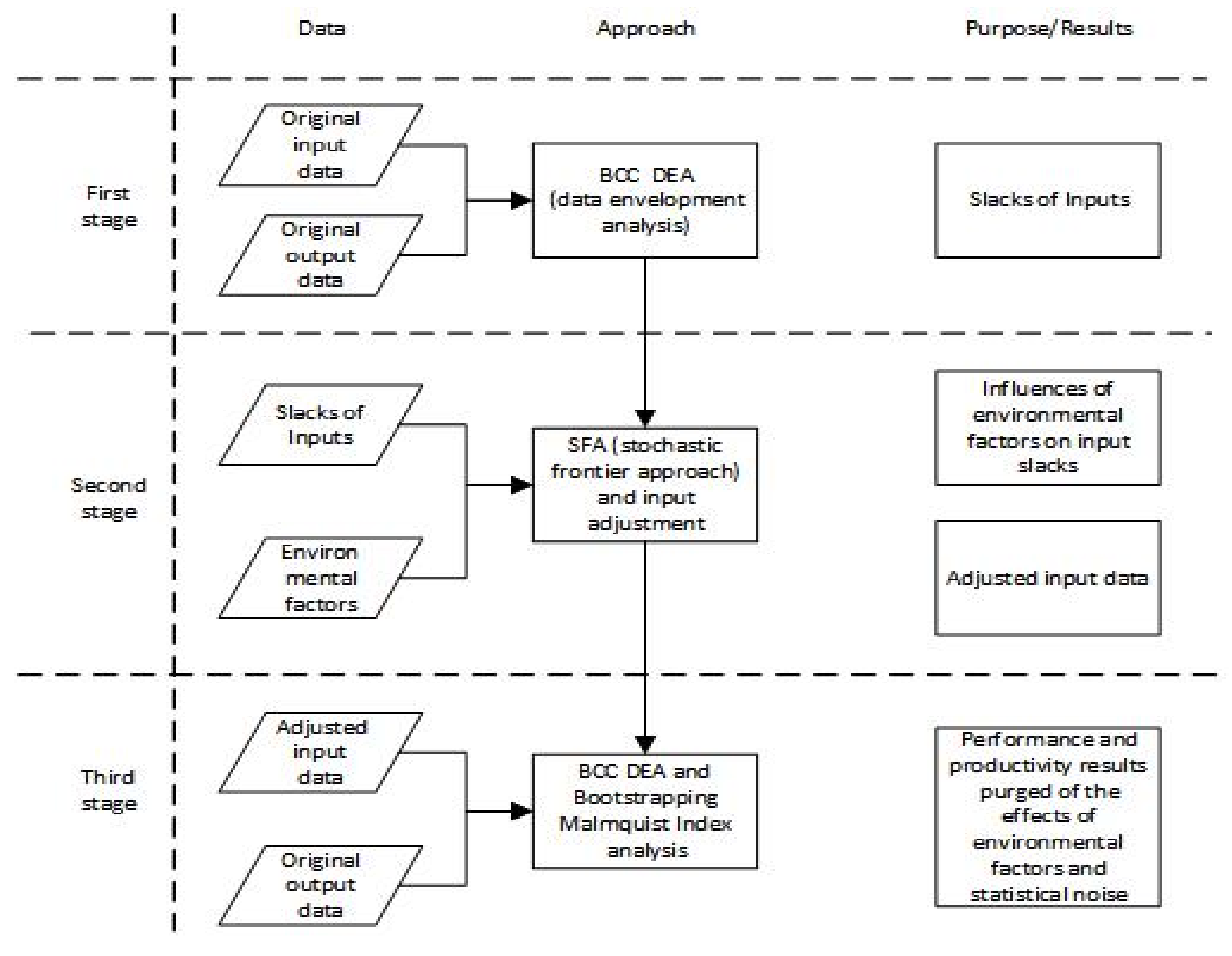
In view of the above two research gaps, this paper constructs an index system of input, output and environmental variables for performance evaluation of the ATS, and adopts a three-stage DEA model [18] that can test and eliminate the influence of environmental factors, to evaluate the “real” performance of regional ATS. The three-stage model combines DEA and stochastic frontier analysis (SFA). It is an adjusted model of the four-stage DEA method by Fried, Schmidt [21]. It is worth noting here that, although SFA is another commonly used parametric performance evaluation method, the purpose of SFA used in this paper is not to directly evaluate performance, but to be used as a regression model in the second stage. The role of the SFA is to identify and quantify the impact of operating environment on the input slacks obtained by first stage DEA.
The remainder of the paper is structured as follows. Section 3 presents a brief introduction to the methodology applied in this research. Section 4 describes the indicators and data sources, including the input and output variables, as well as the environmental variables. The empirical results are presented in Section 5 is concluding remarks.
2. Methods
A three-stage DEA-based model and bootstrap-Malmquist productivity index method are applied in this research, as shown in Figure 1.
2.1. The Three Stage DEA Model
At the first stage, the initial efficiency evaluation based on variable returns to scale (VRS) is conducted with a BCC DEA analysis [22], using input and output quantity data only.
The BCC model is modified from the CCR linear program introduced by Charnes, Cooper, and Rhodes [23]. Let represent the kth decision making unit (DMU) input vector of m inputs in period t, , and let represent the ’s output vector of q outputs in period t, . Under a panel of regions and time periods, the contemporaneous production technology can be expressed as follows:
Then, the input-based directional distance function is defined as follows:
is the Farrell [24] input efficiency and equals the proportional contraction in all inputs that can be feasibly accomplished given the level of outputs, if the DMU adopts contemporaneous frontier production technology in period t.
Then, under the constant returns to scale (CRS) assumption that DMUs cannot or change their scale (or size) of operations, CCR linear programming formula can be expressed as:
where is the amount of ith input to unit j in period t, is the amount of rth output from unit j in period t, n is the number of DMUs, m is the number of inputs, q is the number of outputs. and are the ith input and rth output of the being evaluated in period t. is j-dimensional weight vector of the in period t. CCR optimal solution value indicates the estimation of technical efficiency (TE).
Compared with the CRS assumption of CCR model, BCC model only adds the convexity constraint of , which allows it take variable returns to scale (VRS) into consideration. Note here that since our concern is the extent to which resource inputs can be reduced in order to achieve technical efficiency without any reduction in air transport capacity, input orientation BCC DEA model is adopted. The BCC model can be expressed as:
The objective value of the liner program (4) indicates the pure technical efficiency (PTE). Based on TE calculated from the CCR linear program and PTE from BCC model, Scale Efficiency (SE) can be calculated by .
Note here that the CCR model is used only for the separation of scale efficiency and the estimation of DMUs’ returns to scale. Due to the assumption of various returns to scale in this research, in the first and third stage of the three-stage model in this research, BCC DEA model is employed to evaluate the ATS efficiency.
Then in period t, the quantities of ith input factor’s total slack (radial plus non-radial) to unit j, , can be gained from the results of the BCC model in the first stage. illustrates the difference between the existing inputs and the ideal inputs to achieve the optimum efficiency of each DMU.
At the second stage, the input slacks gained from the first stage BCC analysis are regressed against observable environmental variables and a composed error term by stochastic frontier approach (SFA) regression analysis for each period t. In such a SFA regression model, the regression equations can be expressed:
where is a vector representing the environmental variable vector affecting the efficiency of the jth DMU in period t, . is the coefficient vector of environmental variable. can calculate the environmental values which affect each DMU’s inputs, is the composed error term, and are uncorrelated variables, reflects the managerial inefficiency component for the ith input of the jth DMU in period t and , reflects statistical noise for the ith input of the jth DMU in period t and . Therefore, the role of the SFA is to decompose the first stage slacks into environmental influences, managerial inefficiencies and statistical noise.
Then each DMU’s adjusted inputs are calculated from the results of SFA regressions by means of:
where and are adjusted and observed input quantities in period t, respectively, is estimated values for by the SFA approach. The first adjustment on the right side of Equation (4), , puts all DMUs in a common operating environment. The second adjustment, , puts all DMUs in the same state of nature. In order to obtain estimates of for each DMU, by using the Jondrow, Knox Lovell [25] and Fried, Lovell [18] methodology, estimators of statistical noise residual can be calculated by:
where the conditional estimators for managerial inefficiency is given by . Then inputs adjusted for the impacts of both the observable environmental variables and statistical noise can be obtained by:
Stage 3 is a rerunning of BCC DEA model, using adjusted inputs and original outputs. The result of Stage 3 is a DEA-based evaluation of “real” performance couched solely in terms of managerial efficiency, purged of the effects of the operating environment and statistical noise.
2.2. The Malmquist Productivity Index and Bootstrap-Malmquist Approach
Then the adjusted inputs and original outputs are used to calculate the Malmquist productivity index. Fare, Grosskopf [26] developed a DEA-based Malmquist productivity index (MPI) to calculate the total factor productivity index (TFPI) overtime, as shown in Equation (9):
where y represents the output vector, and x is the input vector. is the input distance function defined in Equation (2). measures the total productivity changes between period t and period with reference to the frontier technology at period t. The total productivity improves if , remains unchanged if , and declines if . The TFPI can be further decomposed into two components: the technical efficiency change index (TECI), which measures “catching up” to the frontier isoquant between period t and period ; and the technological change index (TCI), which captures the frontier isoquant from one period to another. That is, Equation (7) can also be rearranged as the product of catch-up (TECI) and frontier shift (TCI) as shown in Equation (10):
The TECI indicates whether an DMU has moved closer to, or further from, the frontier technology over the study period. It is related to DMU’s efforts for improving its efficiency. The TCI reflects the change in the efficient frontiers between two time periods, which is mainly due to improvements in technological level.
However, since the DEA-based Malmquist index estimators are obtained from observed finite samples, the corresponding measures of efficiency may be sensitive to the sampling variations of the obtained frontier [27,28]. To address this problem and provide a statistical basis for the model applied, we use the smooth bootstrapping method proposed by Simar and Wilson [27] and Simar and Wilson [28], to approximate the sampling distribution of the unknown true values of MPI, and get the bootstrapping MPI estimators. The bootstrapping procedure can be found detailed in the related literatures [27,28].
3. Data
In this research, DMUs are China’s 30 provincial ATSs. Consistent with China’s Industrial Classification for National Economic Activities (GB/T 4754—2017), the ATS referred in this paper consists of air passenger and freight transport, general aviation service, plus air transport support activities, which includes airports, air traffic control and other air transport auxiliary activities. The important fact to note here is that according to accounting standards in air transport industry, major investments, such as aircraft fleets (rolling stock), and the construction of airports and related facilities (infrastructure), are fixed asset investments. This fact serves as an important basis for our selection of input indicators later.
3.1. Input Indicators
Inputs in this research are defined as the resources that ATS take to generate air transport capacity. The capital (rolling stock and infrastructure) and the number of employees (or hours of work) are the most frequently considered variables since they represent the main production process inputs [29]. Air transport is a capital-intensive industry, the measure of capital input is crucial in its efficiency analysis since investments in infrastructure and rolling stock and the cost related to their usage account for a prominent part of firms’ expenses in this industry. Capital input may be considered as either a flow or stock variable. In previous studies the stock index is often used as an input indicator. As stated by Crescenzi, Di Cataldo [30] and Farhadi [31], in order to accurately estimate the growth effect of infrastructure, the capital stock rather than the flow of infrastructure should be used, because it is the stock rather than the flow that really matters for long-term effects. This is especially true for transportation infrastructure, because capital investment requires construction and trial operation to achieve the transportation function, which leads to certain lag. Using stock rather than flow can give more robust results and reduce the reverse causality in empirical models [32,33], which also makes stock a more frequently adopted variable. Furthermore, capital stock can be measured in monetary terms [34,35], or in physical terms, for example, the length, area, or density of road and railway network [30,33]. However, measuring capital inputs in physical units is often accused of posing several issues, as authors use a vast range of variables and it is quite hard to define a unique unit of measure [29].
Therefore, in this research we use the monetary measure of capital stock as the proxy of capital input. We apply the perpetual inventory method [36,37], which is most widely used and considered as the most correct approach in measuring stocks of fixed assets [29], to estimate each province’s ATS capital stock. For each province, the net ATS capital stock at the end of current period can be calculated by:
where is the ATS fixed-asset investment in the current period, while is the depreciation rate. Each province’s annual data on comes from China Statistical Yearbook [38] and Statistical Yearbook of the Chinese Investment in Fixed Assets [3].
In this research we assume ATS capital stock depreciates at a constant rate . As to the value of , we use the comprehensive China infrastructure depreciation rate estimated by previous studies [39,40,41], which is 0.0921. In addition, according to the Perpetual Inventory Method, the estimation of the initial capital stock , in our case the capital stock at the end of 2002, is calculated by:
where is the gross investment in initial year 2002, is the geometric average growth rate of fixed asset investment to the ATS during research period. Based on the collected data between year 2002 and 2012, the value of can be calculated, which is 0.15607.
In terms of labor input, we select the number of full-time employees in ATS as the indicator. Data on this index comes from China Statistical Yearbook of the Tertiary Industry [42].
3.2. Output Indicators
Output variables of the transportation industry typically are in two main categories: transportation services (volume of passenger, freight and vehicles), and transportation value added (GDP of the industry) [43,44,45]. Considering that the output value of air transport is not only reflected in GDP in transportation industry, but also lies in the indirect and catalytic effects of passenger and freight movement on other industries, the volume of passenger, freight, and vehicles are used as three output variables of provincial ATS. The data are collected from website of Civil Aviation Administration of China (CAAC) (http://www.caac.gov.cn/ accessed on 30 December 2020). Starting from 2017, CAAC reported each province’s annual air transport passenger and freight throughput. For years prior to 2017, we follow the same method adopted by the CAAC and add up throughputs of all civil airports in a province to get each province’s air transportation throughput.
3.3. Environmental Variables
It has been theoretically and empirically demonstrated that some social and economic factors affect air transportation, which are referred to as environmental variables in this study. Firstly, since an increase in economic income leads to an increase in economic activity and affects the demand for air passenger and freight transport [46], the gross domestic product (GDP) per capita is selected as an environmental variable. Secondly, because of the relatively high price of air transport service, the regional consumption level has a significant impact on air passenger and cargo transport volume [47,48]. Therefore, we choose household consumption expenditure (HCE) as the second environmental variable. Thirdly, due to the high dependence of R&D industries and other “on-time” technology-intensive industries on air transport services [49], and considering technological development level’s impacts on the operational efficiency of air transport, in this research three kinds of patent granted per 10,000 people is selected as an environmental variable to express provincial scientific and technological level. Fourthly, Balsalobre-Lorente, Driha [50] traced long-run asymmetry relationship and strong connection between economic growth and tourism industry in conjunction with the ATS. This strong connection between tourism and availability of air transport is also supported by the studies of Gallego and Font [51] and Khan, Dong [52]. Thus, the number of inbound tourists is selected as the environmental variable to measure the tourism industry level. Fifthly, due to its direct demands on air cargo transportation Malighetti, Martini [53], wholesale and retail sector’s value added is used as another environmental variable. Sixthly, air transport is the foundation of global trade and globalization, provides crucial services for international business and cross-border investments [54,55]. Thus, regional openness is assumed to have impacts on air transport demand, and on regional ATS efficiency. Therefore, as the openness indicator, actual utilization of foreign direct investment (FDI) is selected as an environmental variable. Finally, as previous studies of Melo, Graham [56] and Jiang, Timmermans [57] argued, the effect of infrastructure on industries development varies across industry groups and transport modes. Thus, we choose industrial structure as an environmental variable, and use the ratio of the tertiary industry added value to GDP to represent the provincial industrial structure.
In summary, the input, output, and environmental variables of the three-stage DEA approach applied are listed in Table 1.
Note here that following the Fried (2002) method, all seven environmental variables are posited to influence ATS performance, although without assumption of the directions of their impacts [18]. The impacts of the environmental variables will be further investigated in Stage 2 SFA analysis.
4. Results
4.1. First Stage Results
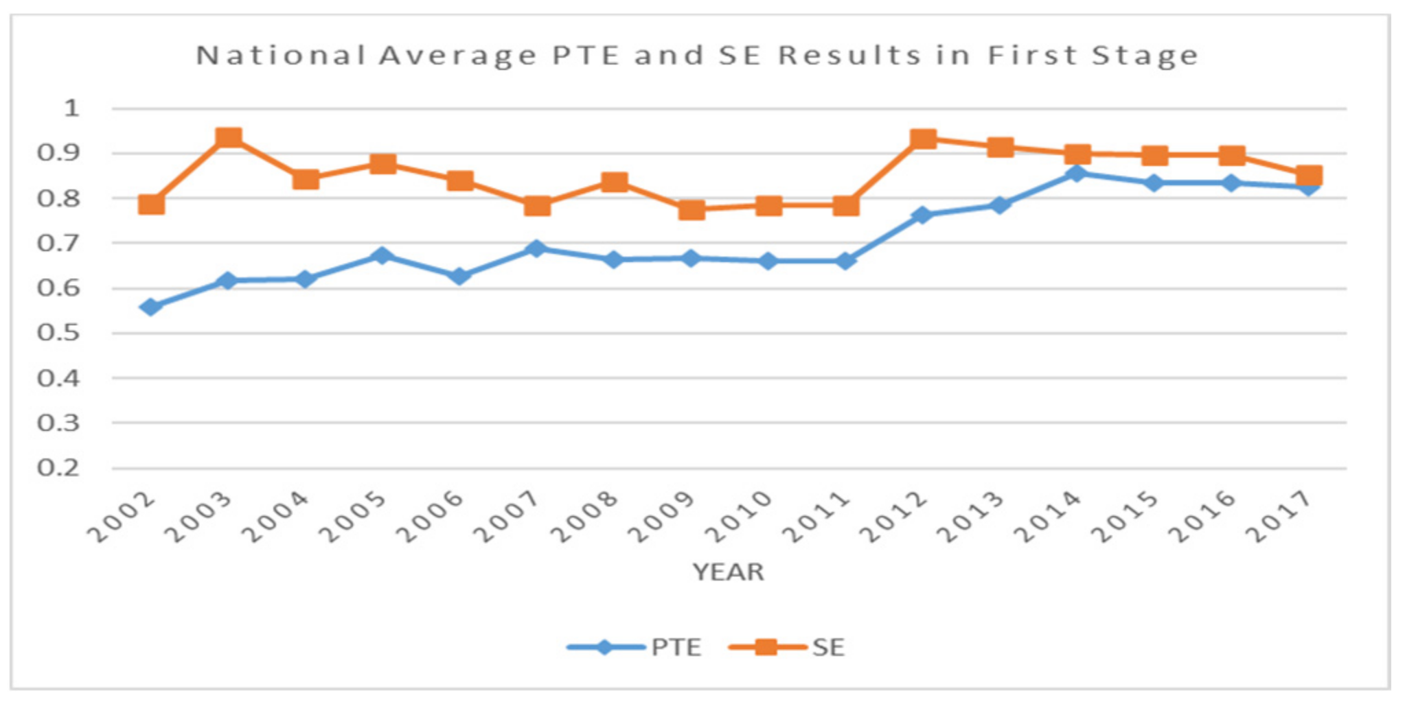
In the first stage, the BCC DEA is applied to evaluate the performance of thirty provinces’ ATS. Table A1 and Table A2 recapitulate detailed results of the first-stage DEA (no adjustment in the environmental variable and statistical noise). The national average PTE and average SE over the 16-year period are shown in Figure 2. Based on the first-stage DEA results, the operating inefficiency is mainly caused by PTE. For comparison purposes, more detailed first stage results will be discussed in the third stage results. Capital and labor input slacks were gained by the first stage BCC model.
4.2. Second Stage Results
The main purpose of second stage is to use SFA to identify the influences of selected macro-economic factors on ATS efficiency, and then calculate the adjusted input values to evaluate real ATS efficiency removing these influences. The SFA regression is utilized to regress capital and labor input slacks respectively, against seven exterior environmental variables, including the GDP per capita, consumption, scientific and technological level, tourism industry, wholesale and retail industry, openness to foreign investment, and industrial structure.
The regression results of the SFA model are demonstrated in Table 2. These results suggest that the environment factors do indeed exert a statistically significant influence on ATS efficiency. In accordance with Table 1, likelihood ratio test values of the regressions for the two input slacks are both higher than the threshold value of the mixed chi-square distribution examination and are at 1% confidence level, rejecting the hypothesis that the one-sided error component makes no contribution to the composed error term, implying the rationality of the stochastic frontier specification [18]. The values of for two regression models are close to 1, which implies that the impact of managerial inefficiency dominates that of statistical noise in the determination of input slack. When examining the impact of environmental variables on input slack variables, if the coefficient is positive, it means that the increase in the value of environmental variables will lead to the increase in input slack variables or the decrease in output, resulting a negative impact on ATS efficiency. If the coefficient is negative, it indicates that the increase of this environmental variable will bring the reduction of input slack or increase of output, which will have a positive impact on the ATS efficiency.
- 1
- GDP per capita
As show in the second row in Table 2, the coefficients of the GDP per capita are positive and significant at 5% level or better in the regression of capital slack and labor slack (127,103.12, and 861.606). This shows that the increase of per capita GDP will lead to the increase of the slack variable of capital and labor input. This may be because the provinces with higher per capita GDP have higher willingness and capacity to invest in air transport, but the resources invested are not fully utilized, which has a negative impact on the efficiency of ATS.
- 2
- Consumption
The coefficients of consumption on capital and labor input slack variables are both negative and significant at the significance level of 1% (−131,960.33, and −2025.766). This shows that higher consumption level is beneficial to air transport operation. Compared with other modes of transportation, air transportation has a higher price. In provinces with high consumption capacity, people are more likely to have a stronger ability to purchase air transportation services, and the resource investment in air transportation can be more easily converted into the growth of passenger and cargo volume, thus avoiding investment waste.
- 3
- Technology level
The regression coefficient of technology level on capital input slack variables is negative and significant at the 1% level (−96,452.384). The improvement of scientific and technological level can improve the operation efficiency of airlines, airports and air traffic control through the application of new technology and equipment and the improvement of management level. This shows that it is reasonable to adhere to the strategy of building “smart airport” and “smart civil aviation”, which is conducive to the improvement of the overall efficiency of ATS. Another reason may be that, as pointed out in the previous literature, technology intensive industries, such as high-tech manufacturing and R&D, are more dependent on air transport services, which will lead to more demand for air transport, thus reducing input redundancy.
- 4
- Tourism industry
The coefficient of tourism level on capital input slack is positive and significant at 1% level (49,024.917). ATS is an important transportation foundation of tourism industry. Provinces and cities rich in tourism resources and focusing on the development of tourism are more inclined to invest in ATS to improve their urban image and facilitate tourism industries. Large-scale input of resources leads to increased input slack. Therefore, at the present stage, although tourism provides the volume demand for the ATS, it does not necessarily bring the improvement of air transport efficiency. Especially under the strategy of moderately advanced construction, provinces and cities need to pay attention to the improvement of ATS efficiency while increasing investment.
- 5
- Wholesale and retail industry
The regression coefficient of the wholesale and retail level to the capital input slack variable is negative, while the coefficient of the labor input slack variable is positive, both of which are significant at the significance level of 1% (−36,260.115 and 1519.889, respectively). This shows that higher level of wholesale and retail can lead to the reduction of capital input slack, and lead to the increase of labor input slack. More developed wholesale and retail industries can bring business volume to air transport, and previous studies have demonstrated that transportation infrastructure serves as the basis for the development of wholesale and retail industries [53]. Better civil aviation infrastructure can also help enterprises to better maintain contact with upstream and downstream dealers, grasp market information faster and more accurately, and expand the market. The mutual promotion mechanism between wholesale and retail and air transport makes this environmental variable have significant effect.
- 6
- Openness to foreign investment
The regression coefficient of openness to foreign investment on capital and labor input slack variables are both negative and significant at 10% level or better (−2859.904, and −292.306). The increase in the degree of openness to foreign capital will significantly reduce the input slacks of capital and labor. The decrease in the input slacks of capital and labor is attributed to a benevolent environment for ATS supported by sufficient openness. Foreign enterprises need air transportation to maintain domestic and foreign relations, and their production and sales activities often rely on international trade. All these demands for civil aviation can make the investment in air transportation more efficient.
- 7
- Industrial structure
The regression coefficient of the industrial structure on capital and labor input slack variables are both negative and significant at the 5% level or better (−122,923.98, and −385.309). This shows that the increase of the proportion of the tertiary industry will lead to the decrease of capital and labor input slacks. Previous studies [50,56] have suggested that air transport contributes more to the growth of the tertiary industry. From the economic perspective of improving the input-output ratio of airlines and airports, the spatial layout and subsidy of the new airlines and airports should be inclined to the cities with better tertiary industry foundation. The results of this study show similar conclusions from another direction. The tertiary industry is more dependent on air transport, and the developed tertiary industry can indeed bring higher input-output ratio to air transport and improve the efficiency of air transport.
The original inputs are then adjusted to account for the effects of variation in the operating environment and in statistical noise, by separating managerial inefficiency component and statistical noise item utilizing the SFA approach. The values of capital and labor input variables are adjusted by Equation (7), excluding the exterior environmental values and statistical noise through substituting the coefficients values , in Table 2 into Equations (5) and (6). Provinces with relatively unfavorable air transport operating environments and relatively bad luck have their inputs adjusted downward by a relatively small amount, while provinces with relatively favorable operating environments and relatively good luck have their inputs adjusted upward by a relatively large amount [18].
4.3. Third Stage Results
At the third stage, based on the adjusted inputs from the second stage and the original outputs, we can estimate the efficiency again with BCC DEA model. This final evaluation put all provinces on a level playing field and can reflect the actual ATS performance, since variation in operating environments and the vagaries of luck have been accounted for.
- Pure technical efficiency (PTE)
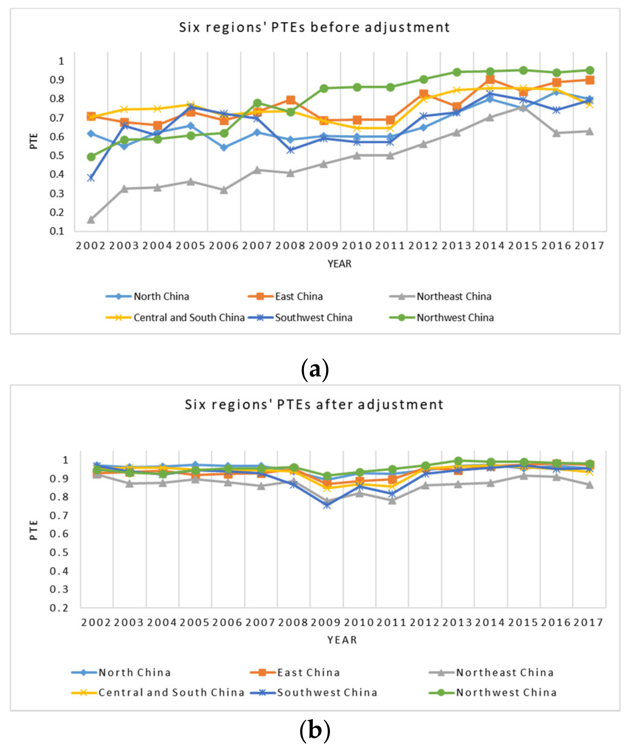
Table 3 listed the polished PTE of the 30 provincial air transport industries. After excluding the influences of exterior environmental factors and statistical noise, 25 out of 30 provinces have improved their PTE values in the evaluation results of the third stage (Table A1 in Appendix A, Table 3). Four provinces were found to be best performers over the entire study periods having consistently full DEA PTE indexes (i.e., Shanghai, Guangdong, Henan, and Qinghai). The civil aviation administration of China (CAAC) has divided China’s air transport into six regions, namely North China, Northeast China, East China, Central and Southern China, Southwest China, Northwest China, each of which consists of several geographically adjacent provinces. Regional administration was set up for each region. Before the adjustment, the six regions’ average PTE indexes over the study period are 0.6610, 0.7617, 0.4810, 0.7568, 0.6680 and 0.7899, respectively. After the adjustment, they are 0.9546, 0.9373, 0.8684, 0.9356, 0.9160 and 0.9597, respectively. This indicates that in the BCC DEA method, the PTE indexes of most provinces are underestimated because the differences in environmental factors are not considered. In addition, after the adjustment, the six regions’ relative ranking in PTE has changed greatly. As shown in Figure 3a, in the first stage, the PTE is highest in Central and Southern China before 2009, and highest in Northwest China after 2009. In the third stage, the PTE value is the highest in North China before 2008, and highest in Northwest China after 2008. However, as shown in Figure 3b, after the adjustment, the gap of pure technical efficiency among each region narrows. After removing the influence of environmental factors, the PTEs of the ATS in each region have improved, and the relative differences among provinces in each year over the study period have narrowed.
As stated in previous study [58,59], when evaluating industrial competitiveness or efficiency, the average efficiency of the ATS during one particular year compared to other years is very important, as this would indicate whether any year was the best performing year with respect to overall industrial efficiency. As Figure 3b shows, in 2009, 2010 and 2011, there is a decline in ATS PTE in all six regions, and it reaches the low point over all 16 years. This is consistent with the practice that, after the 2009 financial crisis, China adopted large-scale infrastructure investment plan, including large scale air transport investment, to boost the economy. During this period, the investment into China’s civil aviation industry increased significantly. However, the payoff of transportation investment had a certain lag effect, and passenger and cargo traffic did not increase in parallel to the increasing inputs. Therefore, the efficiencies in 2009 and the following two years are significantly lower than the other years.
- Scale efficiency (SE)
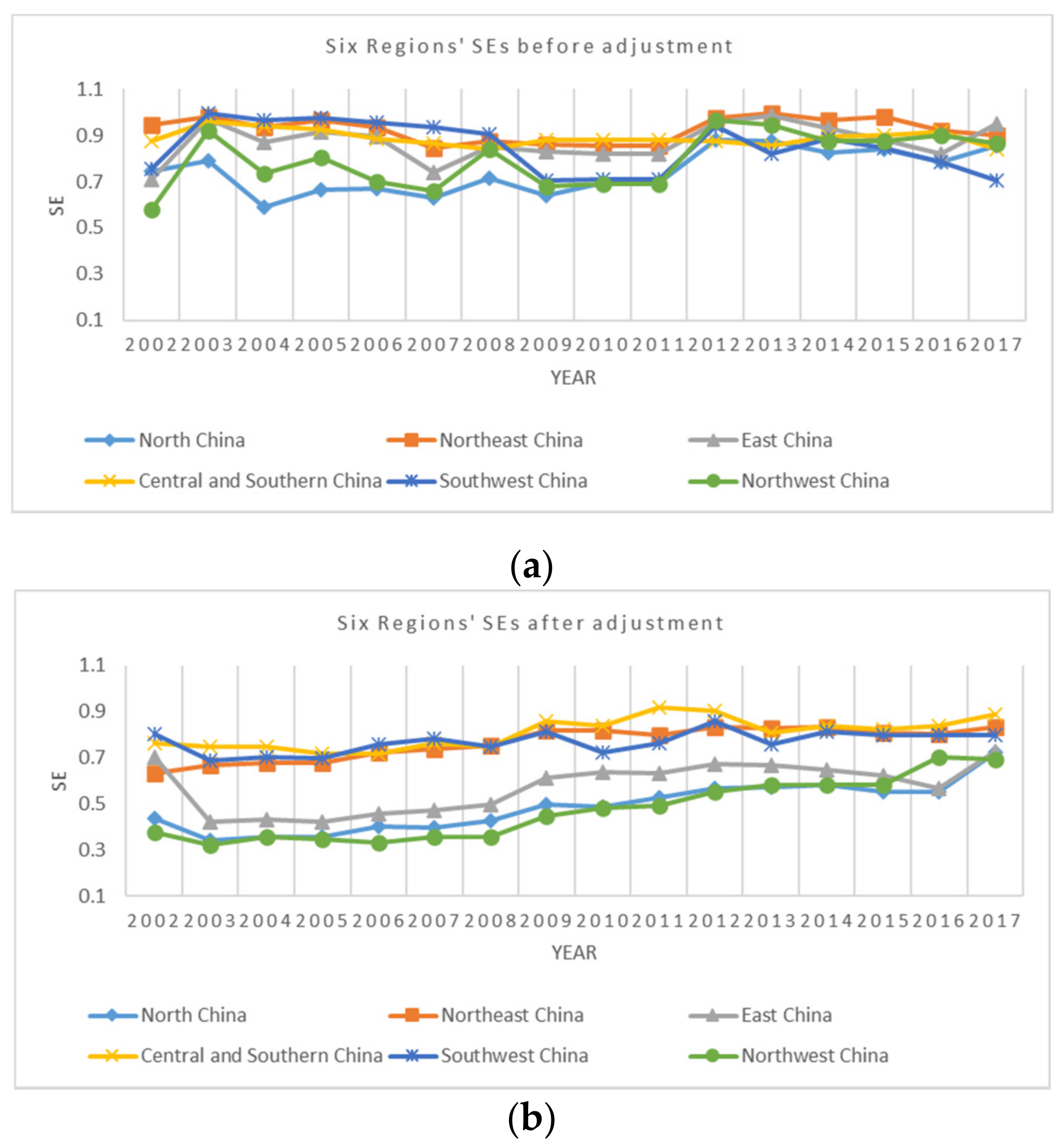
As shown in Table A2 and Table 4, after the adjustment, the scale efficiency of 25 out of 30 provinces have decreased, and the overall level of SE gets lower (Figure 4a,b). These changes in SE caused by this adjustment can also be clearly seen from Figure 3a,b. The average SE values over the study years in North China, East China, Northeast China, Central and southern China, Southwest China, and Northwest China are 0.807, 0.768, 0.765, 0.574, 0.485 and 0.472, respectively. Between 2002 and 2017, the average SE is much lower than the average PTE (Figure 3b and Figure 4b).
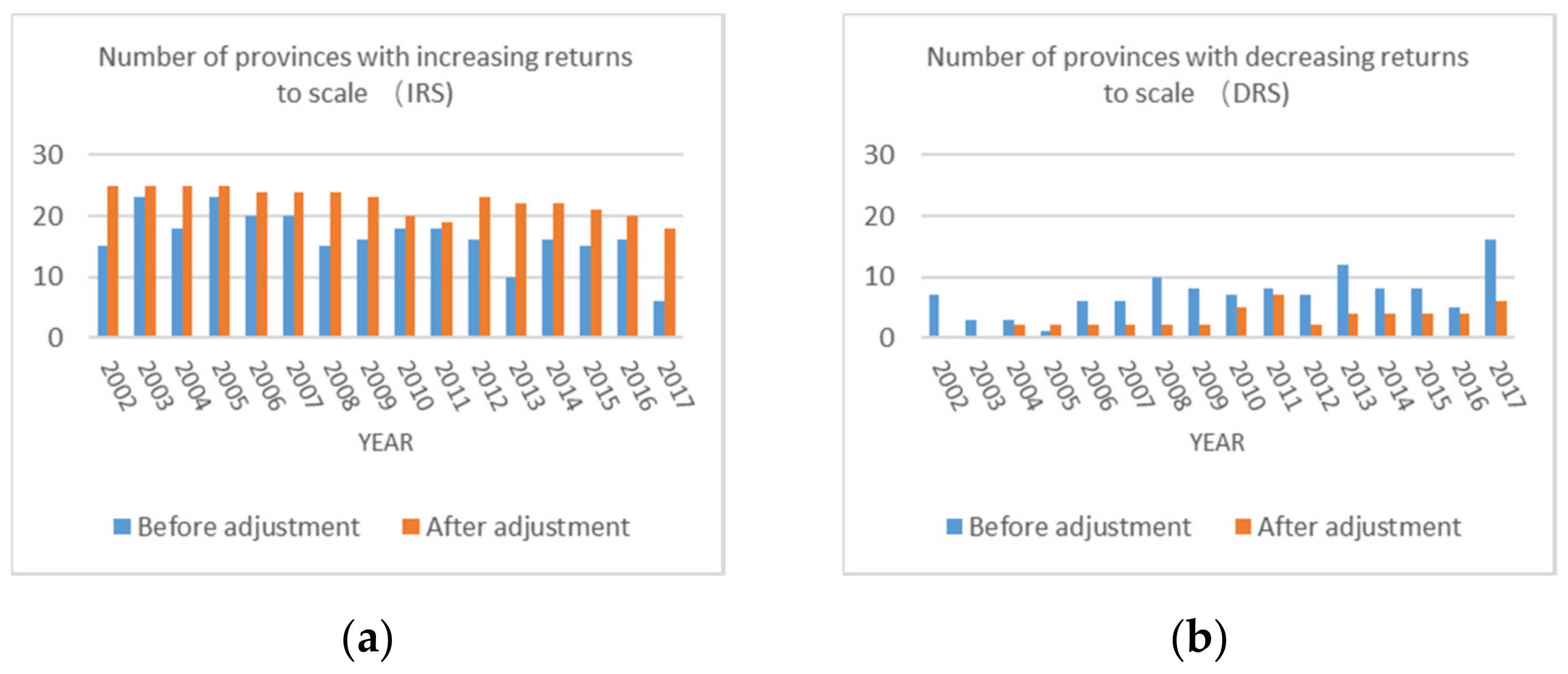
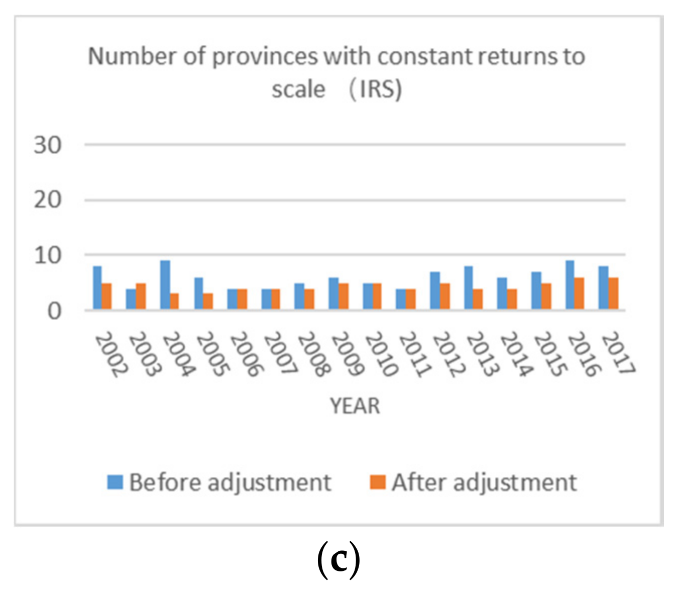
This shows that compared with PTE, SE is the main factor restricting the investment efficiency of the ATS in most provinces. In this study, the efficiency evaluation is based on BCC model, which assumes variable returns to scale (VRS). Thus return-to-scale categories (increasing returns to scale, constant returns to scale, or decreasing returns to scale) of each DMU can be determined. As shown in Figure 5a, after the adjustment, the number of DMUs operating at IRS increases significantly. Each year the number of DMUs at IRS is higher than before the adjustment. The numbers of provinces at DRS and CRS decrease significantly. After adjustment, in each year the number of provinces at DRS is less than that before the adjustment except 2005 (Figure 5b), and the number of provinces at CRS is less than or equal to that before the adjustment except 2003 (Figure 5c).
It is also showed that PTEs of most provinces are underestimated, while SEs of most provinces are largely overestimated since the differences in environmental factors are not considered in BCC DEA model. After adjustment, SE emerged as the main factor restricting the efficiency of the ATS.
Combined with the above results of scale efficiency and returns to scale, it can be told that China’s civil aviation infrastructure and airline networks still have room for expansion, and the air transport market is not yet saturated. Under the expected growth rate of air transport demand, civil aviation development can still be achieved by expanding the resource inputs. The “moderately advanced” development strategy currently adopted by the CAAC is reasonable. After the Localization Reform of Civil Aviation in 2002, with the removal of a series of strict regulatory restrictions, the investment and financing channels for civil aviation development were largely expanded. Meanwhile local governments often have huge enthusiasm in investing on local airports and local airline companies for various economic and political motivations. Between 2002 and 2017, local governments were actively increasing investment in air transport, and the scale of China’s civil aviation construction unprecedentedly grew. However, despite the rapid expansion, the scale efficiency of the ATS is relatively low. Considering the reality in China, the ATS’s low scale efficiency can be improved through the development of more productive aviation network, by which the utilization of aviation infrastructure, especially regional and remote airports and local airlines can be optimized. Therefore, the central civil aviation administration should have long-term strategic vision, pay attention to the overall layout planning and resource allocation among provinces while expanding scale.
Considering the recentness, in year 2017, six provinces (Inner Mongolia, Shanghai, Jiangsu, Zhejiang, Henan, and Shaanxi) are fully scale efficient. Meanwhile, 18 provinces’ ATSs are operating at IRS, which means that that an increase in inputs could realize a more than proportional increase in outputs. So, they could attain better performances by moving towards the scale efficient size based on the currently available technology. The other six provinces (Beijing, Shandong, Guangdong, Sichuan, Yunnan, Xinjiang) are operating at DRS, indicating that an increase in inputs could realize a less than proportional increase in outputs. Four of these (Beijing, Guangdong, Sichuan, Yunnan) are among the top five provinces with largest air transport passenger volume. At first impression, this recommends reducing the scale of these very largest provincial ATSs. So, they could attain better performances by moving towards the scale efficient size based on the currently available technology. A better alternative explanation is modifying airspace limitations and regulatory conditions that impose significant constraints on these provincial ATSs as they grow. For example, these provinces are some of the regions with greatest air transport demands, largest air traffic volumes and steady growth rate. However, due to the limitation of airspace resources, the scale efficiencies and returns to scale of their ATSs are heavily constrained. More scientific and effective utilization of airspace resources can improve the scale effect and efficiency, such as optimizing and integrating traffic flow trend along the air routes, and appropriate use of large and medium-sized aircraft. In addition, new navigation technology and air traffic control technology should be adopted to improve the automation level and reduce the chance of flight delay.
4.4. The Results of Bootstrap-Malmquist Productivity Model
Using the input–output index value calculated in the second stage, the smooth bootstrapping procedure for Malmquist index calculation is implemented. The bootstrapping time is set to 2000. The mean value of the Malmquist index bootstrap adjusted results is calculated using geometric mean. The bootstrap adjusted values of total factor productivity index (TFPI), technical efficiency change index (TECI), and technological change index (TCI) are gained to analyze the productivity change.
- The outline of the air transport productivity change
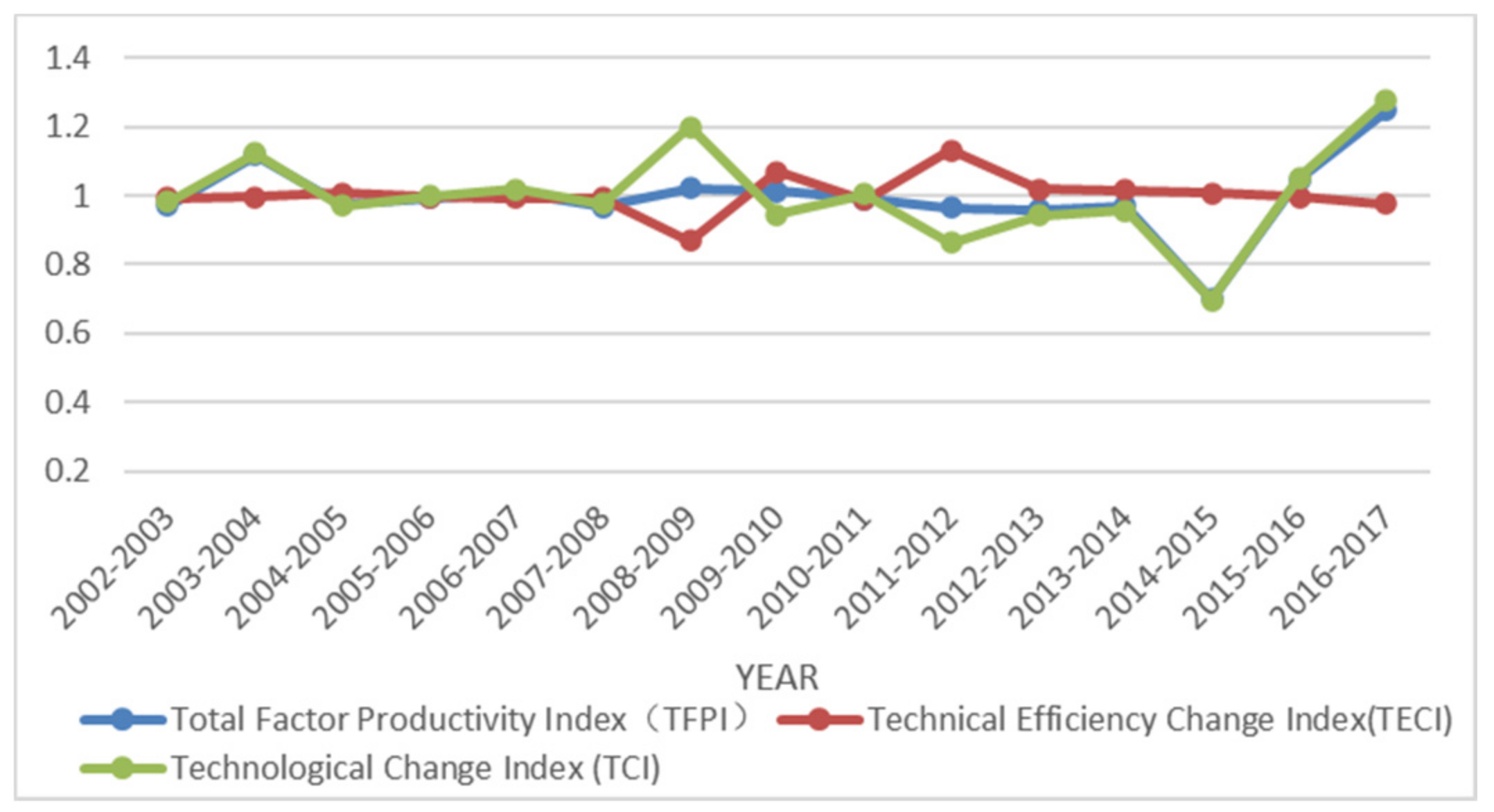
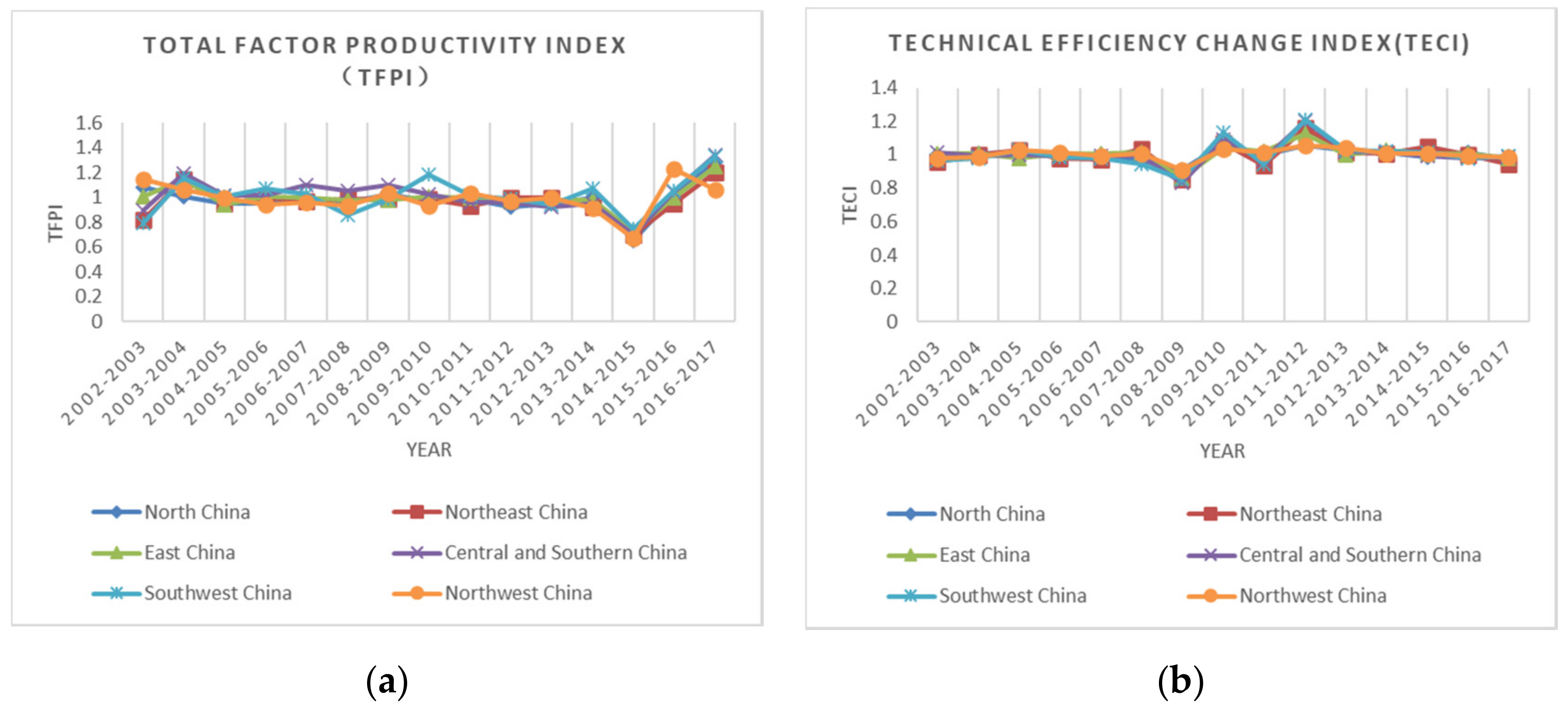
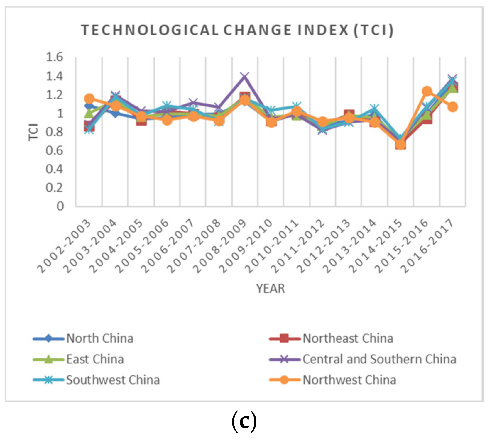
Detailed results of the TFPI, TECI, and TCI are shown in Table A3, Table A4, and Table A5. As displayed in Figure 6, bootstrap adjusted TFPI and TCI exhibit similar patterns over the 16 years span. Although TECI exhibits a significantly different pattern after 2008, technological change serves as the main cause of the TFPI pattern. This result indicates that productivity of air transport is influenced by a technological change more heavily than a technical efficiency change. This is true not only for the national average (Figure 6), but also for each of the six regions (Figure 7).
- Total Factor Productivity Index (TFPI)
As shown in Table A3, national average ATS productivity decreases slightly by 0.3% from 2002–2017. Although the air traffic volume of China has increased significantly during this period, the ATS was also invested with a huge number of resources, and overall, the ATS productivity does not gain significant increase yet. Seven provinces, including Inner Mongolia, Zhejiang, Fujian, Henan, Hainan, Yunnan, Ningxia have experienced increases in total productivity by 0.9%, 6.9%, 1.2%, 10.5%, 1.3%, 3.1%, 0.4%, respectively between 2002 and 2017, whereas the other 23 provinces have experienced declines in total productivity during the study period. Compared with countries with developed air transport system, China’s ATS is still in a period of rapid expansion, and airports, airlines and related ATS auxiliary facilities were, and still are attracting a lot of resource inputs. Therefore, from the perspective of input-output efficiency, the productivity of the ATS has not improved significantly.
- Technical Efficiency Change Index (TECI)
Table A4 summarized the bootstrap adjusted TECI results over the study period. As shown in Figure 7b, TECI in six regions saw a zigzag rise between 2007 and 2013. After five years of rapid investment and expansion from 2002, China’s civil aviation industry began to pay attention to the improvement of its own management and resource utilization in 2007. Although this industry still drew a lot of investment during 2007 to 2013, TECI still showed improvement thanks to the improvement of management level. However, due to the 2009 crisis and its lagged impacts, air transport demand failed to get steady growth, and the overall growth pattern from 2007 to 2013 showed a zigzag trend (Figure 7b). This is in consistent with the research of Örkcü, Balıkçı [6], which concluded that after rebounding in 2010 over the 2009 depression, the world air traffic increase stagnated until 2013.
- Technological change Index (TCI)
Table A5 summarized the changes of TCI over the study period, which don’t show consistent increase until 2014. As shown in Figure 7c, TCI across all six regions experienced increase during the last three consecutive years of the study period, and peaked in 2017. Technical change is often triggered by external factors such as shifts in government policies, advances in technology, and changes in economic environments [6,7]. Following the Next Generation Air Transportation System (NextGen, https://www.faa.gov/NEXTGEN accessed on 30 December 2020) of the USA and Single European Sky ATM Research (SESAR) in Europe, the CAAC launched the modernization of China’s air transportation system to make air transport more efficient. It proposed civil aviation technological development portfolio encompassing the planning and implementation of new technologies, such as automation, information, and intelligence technologies. As a result, ATS saw sustained growth in TCI in recent years. The technology development strategy of China’s ATS began to show effects between 2014 and 2017, with TCI continuously improving and reaching apex, as shown in Figure 6 and Figure 7c.
5. Conclusions and Discussion of Policy Implications
The efficiency and productivity evaluation of ATS is not only affected by direct inputs and outputs, but also by exterior economic and social environment and statistic noise. To overcome the drawbacks of deterministic DEA method, this study applies a three-stage model to evaluate regional ATS performance and productivity. This model takes variable measurement errors and unobserved but potentially relevant variables into consideration by a stochastic disturbance term in SFA. Meanwhile features of the operating environment are taken into consideration by the introduction of seven environmental variables. In order to measure the resource input more accurately, the perpetual inventory method is used to calculate the capital input of the ATS. The bootstrapping Malmquist productivity index is adopted to analyze ATS productivity change over time.
The empirical results show that, environmental factors pose significant influences on ATS performance. Scale efficiency is shown to be the main factor that restricts the efficiency of China’s ATS. Compared with developed countries, China’s ATS is still at the stage of increasing scale benefit. Nearly two-thirds of the DMUs are operating at an insufficient scale. Combined with the results of scale efficiency and returns to scale, most provinces’ ATSs are still at the stage of increasing scale benefit. However, six provinces are at DRS, with four of these provinces (Beijing, Guangdong, Sichuan, Yunnan) having largest provincial air transport passenger numbers. While China’s ATS is experiencing dividends from expansion, special attention should be paid to the coordinated planning and balanced development of air transport in different regions to improve scale efficiency. Bootstrap-Malmquist productivity index results indicate that ATS TECI has not improved significantly in recent years. This can also give the policy inspiration that the management practice still has room for improvement [7]. For example, in practice, the organizational structure and management of airports and airlines can be improved to enhance their public-private cooperation in finance, operation and other aspects. Moreover, technological change determined the trend of ATS total factor productivity in China (Figure 7a,c). This result is similar to the findings of Ahn and Min [7] and Örkcü, Balıkçı [6]. They both found that total factor productivity in the airport industry is mainly influenced by the TCI. Since the TCI is often triggered by external factors such as R&D, innovation, and technological progress [60,61]. This result supports the legitimacy of China’s air transport modernization policy as well as ATS technological development strategy [62], which has resulted in increasingly enormous investment into ATS technological development in the past few years. This technology-oriented industrial development strategy has enhanced the productivity of China’s ATS. In addition to technological innovation and progress, there are some other major external changes that will affect TCI, such as government policies shifts, and changes in economic environment, etc. [6,7]. Additionally, the severe impact of the Covid-19 outbreak on global air transport industry shows us that major social changes, such as public health events, can also be determinants of TCI and ATS productivity. Governments and civil aviation industry should pay special attention to changes in the external environment. These external changes, as well as the ability of civil aviation industry to adapt to the changes, exerts an important impact on ATS performance and productivity.
The shortcoming of the method applied in this article is that it only considers the impact of operational environment factors on performance, but fails to consider the impact of other potentially alternative transport modes on the air transport industry, such as high-speed railway (HSR), which is demonstrated in many research literature [63,64,65].
Future research work can focus on developing appropriate methods to consider the different impacts of other transport modes on the air transport industry in different regions when evaluating ATS performance, to obtain a more realistic evaluation result. The research period selected in this paper is before the outbreak of COVID-19, which totally changed the global air transportation industry. Therefore, another more ambitious and challenging direction for future research is to figure out the impact of COVID-19 on the current and future performance of the global air transport industry, and how to mitigate this impact.
Author Contributions
Conceptualization, data, M.S. and G.J.; methodology, software, writing—original draft preparation, M.S.; writing—review and editing, supervision, funding acquisition, G.J. All authors have read and agreed to the published version of the manuscript.
Funding
This research is funded by Interdisciplinary and Innovative International Training Program of Tongji University, grant number 2020XKJC-005.
Conflicts of Interest
The authors declare no conflict of interest.
Abbreviations
| DEA | Data envelopment analysis |
| DMU | Decision making unit |
| TE | Technical efficiency |
| PTE | Pure technical efficiency |
| SE | Scale efficiency |
| IRS | Increasing returns to scale |
| DRS | Decreasing returns to scale |
| CRS | Constant returns to scale |
| SFA | Stochastic frontier analysis |
| TFPI | Total factor productivity index |
| TECI | Technical efficiency change index |
| TCI | Technological change index |
Appendix A

Table A1.
The first stage pure technical efficiency results from BCC model.
| Region | 2002 | 2003 | 2004 | 2005 | 2006 | 2007 | 2008 | 2009 | 2010 | 2011 | 2012 | 2013 | 2014 | 2015 | 2016 | 2017 | Average | |
|---|---|---|---|---|---|---|---|---|---|---|---|---|---|---|---|---|---|---|
| North China | Beijing | 1 | 1 | 1 | 1 | 1 | 1 | 1 | 1 | 1 | 1 | 1 | 1 | 1 | 0.854 | 0.865 | 0.883 | 0.975 |
| Tianjin | 0.333 | 0.631 | 0.741 | 0.649 | 0.623 | 1 | 0.752 | 0.823 | 0.825 | 0.825 | 0.497 | 0.577 | 0.608 | 0.534 | 0.719 | 0.652 | 0.674 | |
| Hebei | 1 | 0.592 | 0.861 | 1 | 0.493 | 0.52 | 0.548 | 0.496 | 0.437 | 0.437 | 0.526 | 0.529 | 0.633 | 0.518 | 0.607 | 0.46 | 0.604 | |
| Shanxi | 0.343 | 0.342 | 0.254 | 0.336 | 0.328 | 0.359 | 0.381 | 0.441 | 0.431 | 0.431 | 0.593 | 0.656 | 0.764 | 0.845 | 1 | 1 | 0.532 | |
| Inner Mongolia | 0.416 | 0.186 | 0.256 | 0.302 | 0.268 | 0.244 | 0.24 | 0.266 | 0.318 | 0.318 | 0.633 | 0.884 | 1 | 1 | 1 | 1 | 0.521 | |
| Mean | 0.618 | 0.550 | 0.622 | 0.657 | 0.542 | 0.625 | 0.584 | 0.605 | 0.602 | 0.602 | 0.650 | 0.729 | 0.801 | 0.750 | 0.838 | 0.799 | 0.661 | |
| Northeast China | Liaoning | 0.149 | 0.364 | 0.389 | 0.412 | 0.358 | 0.367 | 0.4 | 0.333 | 0.353 | 0.353 | 0.445 | 0.44 | 0.393 | 0.418 | 0.469 | 0.535 | 0.386 |
| Jilin | 0.18 | 0.24 | 0.254 | 0.244 | 0.192 | 0.215 | 0.216 | 0.377 | 0.442 | 0.442 | 0.483 | 0.522 | 0.719 | 0.852 | 0.576 | 0.575 | 0.408 | |
| Heilongjiang | 0.163 | 0.369 | 0.357 | 0.434 | 0.411 | 0.69 | 0.607 | 0.662 | 0.71 | 0.71 | 0.758 | 0.911 | 1 | 1 | 0.813 | 0.784 | 0.649 | |
| Mean | 0.164 | 0.324 | 0.333 | 0.363 | 0.320 | 0.424 | 0.408 | 0.457 | 0.502 | 0.502 | 0.562 | 0.624 | 0.704 | 0.757 | 0.619 | 0.631 | 0.481 | |
| East China | Shanghai | 1 | 1 | 1 | 1 | 1 | 1 | 1 | 1 | 1 | 1 | 1 | 1 | 1 | 1 | 1 | 1 | 1.000 |
| Jiangsu | 1 | 0.699 | 0.855 | 1 | 1 | 0.739 | 1 | 1 | 1 | 1 | 1 | 0.979 | 0.997 | 1 | 1 | 1 | 0.954 | |
| Zhejiang | 1 | 1 | 1 | 1 | 1 | 1 | 1 | 1 | 1 | 1 | 1 | 1 | 1 | 1 | 1 | 1 | 1.000 | |
| Anhui | 0.246 | 0.415 | 0.494 | 0.508 | 0.479 | 0.918 | 1 | 0.464 | 0.407 | 0.407 | 0.54 | 0.506 | 1 | 0.702 | 0.843 | 0.79 | 0.607 | |
| Fujian | 0.317 | 0.617 | 0.515 | 0.533 | 0.438 | 0.401 | 0.467 | 0.376 | 0.389 | 0.389 | 0.658 | 0.636 | 0.621 | 0.565 | 0.639 | 0.559 | 0.508 | |
| Jiangxi | 1 | 0.415 | 0.214 | 0.509 | 0.445 | 0.581 | 0.634 | 0.377 | 0.421 | 0.421 | 1 | 0.549 | 1 | 1 | 1 | 1 | 0.660 | |
| Shandong | 0.4 | 0.588 | 0.546 | 0.584 | 0.456 | 0.487 | 0.472 | 0.589 | 0.607 | 0.607 | 0.61 | 0.656 | 0.716 | 0.615 | 0.742 | 0.959 | 0.602 | |
| Mean | 0.709 | 0.676 | 0.661 | 0.733 | 0.688 | 0.732 | 0.796 | 0.687 | 0.689 | 0.689 | 0.830 | 0.761 | 0.905 | 0.840 | 0.889 | 0.901 | 0.762 | |
| Central and Southern China | Henan | 1 | 1 | 1 | 1 | 1 | 1 | 1 | 1 | 1 | 1 | 1 | 1 | 0.967 | 1 | 1 | 1 | 0.998 |
| Hubei | 0.436 | 0.466 | 0.356 | 0.505 | 0.364 | 0.424 | 0.439 | 0.412 | 0.474 | 0.474 | 0.752 | 0.712 | 1 | 1 | 1 | 0.684 | 0.594 | |
| Hunan | 0.504 | 0.635 | 1 | 0.922 | 0.931 | 0.978 | 1 | 0.91 | 0.68 | 0.68 | 0.771 | 0.925 | 0.931 | 1 | 0.977 | 0.723 | 0.848 | |
| Guangdong | 1 | 1 | 1 | 1 | 1 | 1 | 1 | 1 | 1 | 1 | 1 | 1 | 1 | 1 | 1 | 1 | 1.000 | |
| Guangxi | 1 | 0.708 | 0.604 | 0.757 | 0.658 | 0.699 | 0.635 | 0.683 | 0.602 | 0.602 | 0.783 | 0.93 | 0.578 | 0.742 | 0.822 | 0.732 | 0.721 | |
| Hainan | 0.287 | 0.667 | 0.525 | 0.433 | 0.327 | 0.299 | 0.346 | 0.108 | 0.112 | 0.112 | 0.495 | 0.512 | 0.669 | 0.401 | 0.308 | 0.484 | 0.380 | |
| Mean | 0.705 | 0.746 | 0.748 | 0.770 | 0.713 | 0.733 | 0.737 | 0.686 | 0.645 | 0.645 | 0.800 | 0.847 | 0.858 | 0.857 | 0.851 | 0.771 | 0.757 | |
| Southwest China | Chongqing | 0.295 | 0.689 | 0.488 | 1 | 1 | 1 | 0.657 | 0.353 | 0.429 | 0.429 | 0.735 | 0.714 | 0.989 | 0.818 | 0.684 | 0.691 | 0.686 |
| Sichuan | 0.238 | 0.442 | 0.462 | 0.447 | 0.405 | 0.401 | 0.374 | 1 | 1 | 1 | 1 | 1 | 1 | 1 | 1 | 1 | 0.736 | |
| Guizhou | 0.332 | 0.5 | 0.482 | 0.585 | 0.48 | 0.446 | 0.437 | 0.573 | 0.468 | 0.468 | 0.522 | 0.558 | 0.706 | 0.641 | 0.491 | 0.529 | 0.514 | |
| Yunnan | 0.667 | 1 | 1 | 1 | 1 | 0.935 | 0.655 | 0.444 | 0.393 | 0.393 | 0.584 | 0.639 | 0.615 | 0.73 | 0.79 | 0.952 | 0.737 | |
| Mean | 0.383 | 0.658 | 0.608 | 0.758 | 0.721 | 0.696 | 0.531 | 0.593 | 0.573 | 0.573 | 0.710 | 0.728 | 0.828 | 0.797 | 0.741 | 0.793 | 0.668 | |
| Northwest China | Shaanxi | 0.182 | 0.372 | 0.335 | 0.471 | 0.676 | 0.627 | 0.676 | 1 | 1 | 1 | 1 | 1 | 1 | 1 | 1 | 1 | 0.771 |
| Gansu | 0.147 | 0.23 | 0.247 | 0.277 | 0.413 | 1 | 1 | 1 | 0.891 | 0.891 | 1 | 1 | 0.968 | 1 | 1 | 1 | 0.754 | |
| Qinghai | 1 | 1 | 1 | 0.891 | 0.732 | 1 | 1 | 1 | 1 | 1 | 1 | 1 | 1 | 1 | 1 | 1 | 0.976 | |
| Ningxia | 1 | 1 | 1 | 1 | 1 | 1 | 0.729 | 0.96 | 1 | 1 | 1 | 1 | 1 | 1 | 1 | 1 | 0.981 | |
| Xinjiang | 0.142 | 0.329 | 0.353 | 0.392 | 0.284 | 0.281 | 0.254 | 0.325 | 0.421 | 0.421 | 0.533 | 0.719 | 0.773 | 0.77 | 0.704 | 0.772 | 0.467 | |
| Mean | 0.494 | 0.586 | 0.587 | 0.606 | 0.621 | 0.782 | 0.732 | 0.857 | 0.862 | 0.862 | 0.907 | 0.944 | 0.948 | 0.954 | 0.941 | 0.954 | 0.790 | |
Table A2.
The first stage scale efficiency results from BCC model.
| Region | 2002 | 2003 | 2004 | 2005 | 2006 | 2007 | 2008 | 2009 | 2010 | 2011 | 2012 | 2013 | 2014 | 2015 | 2016 | 2017 | Average | |
|---|---|---|---|---|---|---|---|---|---|---|---|---|---|---|---|---|---|---|
| North China | Beijing | 0.793 | 0.502 | 0.301 | 0.316 | 0.247 | 0.286 | 0.311 | 0.312 | 0.434 | 0.434 | 0.47 | 0.554 | 0.521 | 0.54 | 0.542 | 0.502 | 0.442 |
| Tianjin | 0.822 | 0.909 | 0.871 | 0.898 | 0.846 | 0.854 | 0.899 | 0.9 | 0.928 | 0.928 | 0.99 | 0.915 | 0.838 | 0.816 | 0.83 | 0.868 | 0.882 | |
| Hebei | 0.951 | 0.815 | 0.356 | 0.507 | 0.579 | 0.355 | 0.403 | 0.478 | 0.56 | 0.56 | 0.979 | 0.971 | 0.811 | 0.874 | 0.716 | 0.903 | 0.676 | |
| Shanxi | 0.87 | 0.877 | 0.762 | 0.846 | 0.874 | 0.867 | 0.99 | 0.783 | 0.812 | 0.812 | 0.973 | 0.999 | 0.95 | 0.98 | 0.841 | 1 | 0.890 | |
| Inner Mongolia | 0.3 | 0.858 | 0.658 | 0.764 | 0.808 | 0.783 | 0.96 | 0.737 | 0.729 | 0.729 | 0.998 | 0.931 | 1 | 1 | 1 | 1 | 0.828 | |
| Mean | 0.747 | 0.792 | 0.590 | 0.666 | 0.671 | 0.629 | 0.713 | 0.642 | 0.693 | 0.693 | 0.882 | 0.874 | 0.824 | 0.842 | 0.786 | 0.855 | 0.744 | |
| Northeast China | Liaoning | 0.997 | 0.997 | 0.995 | 0.992 | 0.995 | 0.986 | 0.974 | 0.999 | 0.945 | 0.945 | 0.997 | 0.984 | 0.992 | 0.961 | 0.963 | 0.991 | 0.982 |
| Jilin | 0.419 | 0.96 | 0.73 | 0.8 | 0.803 | 0.74 | 0.817 | 0.638 | 0.668 | 0.668 | 0.9 | 0.982 | 0.804 | 0.721 | 0.713 | 0.893 | 0.766 | |
| Heilongjiang | 0.709 | 0.952 | 0.882 | 0.953 | 0.881 | 0.496 | 0.755 | 0.847 | 0.852 | 0.852 | 0.977 | 0.995 | 1 | 0.955 | 0.777 | 0.961 | 0.865 | |
| Mean | 0.708 | 0.970 | 0.869 | 0.915 | 0.893 | 0.741 | 0.849 | 0.828 | 0.822 | 0.822 | 0.958 | 0.987 | 0.932 | 0.879 | 0.818 | 0.948 | 0.871 | |
| East China | Shanghai | 1 | 1 | 1 | 1 | 1 | 1 | 1 | 1 | 1 | 1 | 1 | 1 | 1 | 1 | 1 | 0.964 | 0.998 |
| Jiangsu | 1 | 0.963 | 0.956 | 1 | 0.897 | 0.898 | 1 | 1 | 1 | 1 | 1 | 0.999 | 0.996 | 1 | 1 | 1 | 0.982 | |
| Zhejiang | 1 | 1 | 1 | 1 | 1 | 1 | 1 | 0.839 | 0.835 | 0.835 | 1 | 1 | 1 | 1 | 1 | 1 | 0.969 | |
| Anhui | 0.684 | 0.97 | 0.787 | 0.827 | 0.829 | 0.45 | 0.597 | 0.652 | 0.628 | 0.628 | 0.942 | 0.994 | 0.86 | 0.887 | 0.868 | 0.862 | 0.779 | |
| Fujian | 0.951 | 0.999 | 1 | 0.999 | 0.985 | 0.978 | 0.925 | 0.977 | 0.988 | 0.988 | 0.9 | 0.991 | 0.974 | 0.972 | 0.97 | 0.941 | 0.971 | |
| Jiangxi | 1 | 0.944 | 0.81 | 0.927 | 0.847 | 0.591 | 0.627 | 0.683 | 0.695 | 0.695 | 1 | 0.998 | 0.951 | 1 | 0.757 | 1 | 0.845 | |
| Shandong | 0.975 | 0.999 | 0.999 | 0.996 | 0.996 | 0.995 | 0.981 | 0.875 | 0.856 | 0.856 | 0.999 | 0.987 | 0.983 | 0.997 | 0.847 | 0.528 | 0.929 | |
| Mean | 0.944 | 0.982 | 0.936 | 0.964 | 0.936 | 0.845 | 0.876 | 0.861 | 0.857 | 0.857 | 0.977 | 0.996 | 0.966 | 0.979 | 0.920 | 0.899 | 0.925 | |
| Central and Southern China | Henan | 1 | 1 | 1 | 1 | 1 | 1 | 1 | 1 | 1 | 1 | 1 | 1 | 0.98 | 1 | 1 | 1 | 0.999 |
| Hubei | 0.991 | 0.979 | 0.958 | 0.948 | 0.958 | 0.977 | 0.905 | 0.949 | 0.959 | 0.959 | 0.938 | 0.927 | 1 | 0.996 | 1 | 0.848 | 0.956 | |
| Hunan | 0.959 | 0.991 | 1 | 0.986 | 0.962 | 0.959 | 0.978 | 0.955 | 0.968 | 0.968 | 0.998 | 0.975 | 0.997 | 0.974 | 1 | 0.986 | 0.979 | |
| Guangdong | 0.568 | 0.815 | 0.706 | 0.652 | 0.473 | 0.459 | 0.452 | 0.455 | 0.435 | 0.435 | 0.715 | 0.397 | 0.418 | 0.456 | 0.519 | 0.506 | 0.529 | |
| Guangxi | 1 | 0.993 | 0.981 | 0.979 | 0.947 | 0.941 | 0.977 | 0.923 | 0.933 | 0.933 | 0.994 | 0.954 | 0.973 | 0.989 | 0.992 | 0.997 | 0.969 | |
| Hainan | 0.719 | 0.999 | 0.983 | 0.992 | 0.966 | 0.863 | 0.725 | 0.993 | 0.99 | 0.99 | 0.617 | 0.884 | 0.993 | 0.991 | 0.984 | 0.708 | 0.900 | |
| Mean | 0.873 | 0.963 | 0.938 | 0.926 | 0.884 | 0.867 | 0.840 | 0.879 | 0.881 | 0.881 | 0.877 | 0.856 | 0.894 | 0.901 | 0.916 | 0.841 | 0.888 | |
| Southwest China | Chongqing | 0.949 | 0.994 | 0.978 | 0.995 | 1 | 1 | 0.887 | 0.97 | 0.992 | 0.992 | 0.993 | 1 | 0.993 | 0.991 | 0.973 | 0.867 | 0.973 |
| Sichuan | 0.952 | 0.999 | 1 | 1 | 0.969 | 0.901 | 0.979 | 0.417 | 0.425 | 0.425 | 0.976 | 0.443 | 0.582 | 0.625 | 0.589 | 0.553 | 0.740 | |
| Guizhou | 0.597 | 0.985 | 0.876 | 0.9 | 0.901 | 0.875 | 0.763 | 0.784 | 0.814 | 0.814 | 0.982 | 0.989 | 0.973 | 0.958 | 0.958 | 0.924 | 0.881 | |
| Yunnan | 0.513 | 1 | 1 | 1 | 0.944 | 0.956 | 0.994 | 0.649 | 0.614 | 0.614 | 0.807 | 0.843 | 0.995 | 0.808 | 0.615 | 0.473 | 0.802 | |
| Mean | 0.753 | 0.995 | 0.964 | 0.974 | 0.954 | 0.933 | 0.906 | 0.705 | 0.711 | 0.711 | 0.940 | 0.819 | 0.886 | 0.846 | 0.784 | 0.704 | 0.849 | |
| Northwest China | Shaanxi | 0.987 | 0.996 | 1 | 0.978 | 0.981 | 0.977 | 0.989 | 1 | 1 | 1 | 1 | 1 | 1 | 1 | 1 | 1 | 0.994 |
| Gansu | 0.407 | 0.86 | 0.646 | 0.876 | 0.508 | 0.369 | 0.513 | 0.632 | 0.562 | 0.562 | 0.945 | 1 | 0.854 | 0.918 | 0.902 | 1 | 0.722 | |
| Qinghai | 0.446 | 0.896 | 0.414 | 0.401 | 0.435 | 0.376 | 1 | 0.363 | 0.343 | 0.343 | 1 | 0.726 | 0.667 | 0.631 | 0.64 | 0.457 | 0.571 | |
| Ningxia | 0.345 | 0.856 | 0.635 | 0.82 | 0.647 | 0.642 | 0.725 | 0.5 | 0.616 | 0.616 | 0.903 | 1 | 0.874 | 0.837 | 1 | 0.986 | 0.750 | |
| Xinjiang | 0.709 | 0.99 | 0.983 | 0.949 | 0.94 | 0.935 | 0.986 | 0.903 | 0.93 | 0.93 | 0.989 | 1 | 0.994 | 0.981 | 0.971 | 0.894 | 0.943 | |
| Mean | 0.579 | 0.920 | 0.736 | 0.805 | 0.702 | 0.660 | 0.843 | 0.680 | 0.690 | 0.690 | 0.967 | 0.945 | 0.878 | 0.873 | 0.903 | 0.867 | 0.796 | |
Table A3.
Changes of bootstrapped TFPI over time.
| Region | 2002–2003 | 2003–2004 | 2004–2005 | 2005–2006 | 2006–2007 | 2007–2008 | 2008–2009 | 2009–2010 | 2010–2011 | 2011–2012 | 2012–2013 | 2013–2014 | 2014–2015 | 2015–2016 | 2016–2017 | Average over Study Period | |
|---|---|---|---|---|---|---|---|---|---|---|---|---|---|---|---|---|---|
| North China | Beijing | 0.830 | 0.879 | 0.909 | 0.957 | 0.969 | 0.907 | 1.114 | 1.042 | 1.126 | 1.001 | 0.966 | 1.258 | 0.982 | 0.957 | 0.876 | 0.985 |
| Tianjin | 0.737 | 1.052 | 1.000 | 0.913 | 1.001 | 0.931 | 0.954 | 1.013 | 0.962 | 0.711 | 0.942 | 0.928 | 0.569 | 1.050 | 1.310 | 0.938 | |
| Hebei | 0.983 | 1.086 | 0.911 | 0.925 | 0.961 | 0.981 | 1.056 | 0.868 | 0.981 | 0.976 | 0.891 | 0.888 | 0.485 | 1.058 | 1.539 | 0.973 | |
| Shanxi | 1.504 | 0.953 | 0.976 | 0.987 | 1.000 | 1.028 | 0.987 | 0.966 | 0.953 | 0.945 | 0.994 | 0.938 | 0.648 | 0.940 | 1.165 | 0.999 | |
| Inner Mongolia | 1.326 | 1.060 | 0.948 | 0.968 | 0.986 | 0.962 | 1.024 | 0.944 | 0.936 | 0.960 | 0.967 | 0.956 | 0.566 | 1.022 | 1.512 | 1.009 | |
| Northeast China | Liaoning | 0.935 | 1.222 | 0.982 | 1.034 | 1.027 | 1.027 | 0.999 | 1.043 | 0.804 | 0.921 | 1.015 | 0.973 | 0.658 | 1.059 | 1.277 | 0.998 |
| Jilin | 0.593 | 1.101 | 0.922 | 0.961 | 0.997 | 0.972 | 1.034 | 0.988 | 0.984 | 1.015 | 1.000 | 0.883 | 0.694 | 0.901 | 1.254 | 0.953 | |
| Heilongjiang | 0.940 | 1.109 | 0.954 | 0.995 | 0.878 | 0.964 | 0.934 | 0.936 | 1.005 | 1.045 | 0.968 | 0.919 | 0.758 | 0.883 | 1.079 | 0.958 | |
| East China | Shanghai | 0.994 | 0.999 | 0.946 | 0.876 | 0.918 | 0.998 | 0.947 | 1.108 | 0.994 | 1.042 | 1.005 | 1.050 | 0.899 | 0.917 | 0.973 | 0.978 |
| Jiangsu | 1.132 | 1.163 | 0.896 | 0.871 | 1.076 | 1.053 | 0.996 | 0.942 | 0.926 | 0.962 | 0.890 | 0.880 | 0.884 | 1.017 | 1.195 | 0.992 | |
| Zhejiang | 1.008 | 1.383 | 0.836 | 1.301 | 1.031 | 0.958 | 1.121 | 1.008 | 1.004 | 1.022 | 1.141 | 1.051 | 0.827 | 1.029 | 1.316 | 1.069 | |
| Anhui | 0.954 | 1.111 | 0.932 | 0.984 | 0.919 | 0.929 | 0.883 | 0.902 | 0.929 | 0.949 | 0.932 | 0.939 | 0.568 | 0.982 | 1.231 | 0.943 | |
| Fujian | 0.990 | 1.159 | 0.973 | 1.034 | 1.040 | 1.019 | 0.973 | 1.127 | 1.049 | 0.925 | 0.980 | 0.953 | 0.650 | 1.002 | 1.304 | 1.012 | |
| Jiangxi | 0.860 | 0.984 | 1.044 | 0.948 | 0.938 | 0.962 | 0.892 | 0.944 | 0.960 | 1.034 | 0.839 | 1.011 | 0.620 | 0.924 | 1.206 | 0.944 | |
| Shandong | 1.076 | 1.191 | 0.957 | 1.010 | 1.037 | 0.936 | 1.046 | 1.003 | 1.121 | 0.863 | 1.057 | 0.978 | 0.660 | 1.073 | 1.511 | 1.035 | |
| Central and Southern China | Henan | 0.770 | 1.310 | 1.278 | 0.914 | 1.448 | 1.574 | 1.204 | 1.130 | 0.784 | 1.264 | 0.801 | 0.747 | 0.759 | 1.053 | 1.541 | 1.105 |
| Hubei | 0.890 | 1.105 | 0.996 | 0.969 | 1.057 | 0.925 | 1.162 | 0.935 | 1.012 | 0.884 | 0.944 | 0.996 | 0.604 | 1.052 | 1.482 | 1.001 | |
| Hunan | 0.920 | 1.275 | 0.882 | 1.084 | 1.004 | 0.933 | 1.015 | 0.823 | 0.945 | 0.865 | 0.980 | 0.913 | 0.648 | 1.025 | 1.315 | 0.975 | |
| Guangdong | 0.995 | 1.156 | 1.078 | 1.111 | 1.055 | 1.045 | 1.034 | 1.100 | 1.039 | 1.032 | 0.789 | 1.097 | 0.989 | 1.032 | 1.058 | 1.041 | |
| Guangxi | 0.808 | 1.119 | 0.977 | 0.980 | 0.994 | 0.896 | 1.022 | 0.902 | 0.983 | 0.956 | 0.997 | 0.863 | 0.660 | 1.043 | 1.330 | 0.969 | |
| Hainan | 0.987 | 1.162 | 0.902 | 1.014 | 1.061 | 0.961 | 1.172 | 1.243 | 1.007 | 0.743 | 1.007 | 1.059 | 0.546 | 1.037 | 1.300 | 1.013 | |
| Southwest China | Chongqing | 0.582 | 1.115 | 1.029 | 1.059 | 1.062 | 0.790 | 1.006 | 0.965 | 0.951 | 0.942 | 1.008 | 1.032 | 0.609 | 1.014 | 1.309 | 0.965 |
| Sichuan | 0.948 | 1.235 | 0.949 | 1.082 | 1.018 | 0.946 | 1.185 | 1.713 | 1.136 | 1.209 | 0.661 | 1.196 | 0.981 | 1.042 | 1.218 | 1.101 | |
| Guizhou | 0.732 | 1.124 | 0.940 | 0.997 | 0.983 | 0.943 | 1.020 | 0.889 | 0.955 | 0.866 | 0.993 | 0.965 | 0.583 | 1.024 | 1.325 | 0.956 | |
| Yunnan | 0.903 | 1.136 | 1.094 | 1.132 | 1.022 | 0.762 | 0.733 | 1.175 | 1.002 | 0.939 | 1.085 | 1.077 | 0.797 | 1.120 | 1.489 | 1.031 | |
| Northwest China | Shaanxi | 0.985 | 1.117 | 1.049 | 1.089 | 0.996 | 0.900 | 1.353 | 0.950 | 1.109 | 0.784 | 1.053 | 1.028 | 0.833 | 1.007 | 1.095 | 1.023 |
| Gansu | 1.546 | 1.035 | 1.011 | 0.910 | 0.947 | 0.875 | 0.961 | 0.903 | 0.976 | 0.968 | 0.978 | 0.896 | 0.590 | 0.970 | 1.309 | 0.992 | |
| Qinghai | 1.020 | 1.024 | 0.977 | 0.880 | 0.932 | 0.952 | 0.990 | 0.899 | 0.956 | 0.979 | 0.870 | 0.890 | 0.560 | 0.973 | 1.274 | 0.945 | |
| Ningxia | 1.180 | 1.019 | 0.999 | 0.886 | 0.944 | 0.923 | 0.933 | 0.926 | 1.016 | 1.049 | 0.998 | 0.851 | 0.634 | 2.255 | 0.447 | 1.004 | |
| Xinjiang | 0.972 | 1.137 | 0.941 | 0.958 | 0.984 | 0.990 | 0.918 | 0.988 | 1.115 | 1.057 | 1.062 | 0.887 | 0.750 | 0.934 | 1.161 | 0.990 | |
| National average | 0.970 | 1.117 | 0.976 | 0.994 | 1.009 | 0.968 | 1.022 | 1.013 | 0.991 | 0.964 | 0.960 | 0.970 | 0.700 | 1.047 | 1.247 | 0.997 | |
Table A4.
Changes of bootstrapped TECI over time.
| Region | 2002–2003 | 2003–2004 | 2004–2005 | 2005–2006 | 2006–2007 | 2007–2008 | 2008–2009 | 2009–2010 | 2010–2011 | 2011–2012 | 2012–2013 | 2013–2014 | 2014–2015 | 2015–2016 | 2016–2017 | Average over Study Period | |
|---|---|---|---|---|---|---|---|---|---|---|---|---|---|---|---|---|---|
| North China | Beijing | 0.989 | 0.996 | 1.011 | 0.987 | 0.995 | 0.995 | 0.900 | 1.048 | 0.994 | 1.086 | 1.011 | 1.018 | 0.906 | 1.004 | 1.023 | 0.998 |
| Tianjin | 0.932 | 1.097 | 0.971 | 0.990 | 1.034 | 0.930 | 0.949 | 1.110 | 1.015 | 0.895 | 1.036 | 1.012 | 1.021 | 1.037 | 0.917 | 0.996 | |
| Hebei | 1.132 | 0.998 | 1.002 | 1.013 | 0.984 | 0.943 | 1.003 | 0.975 | 1.021 | 1.070 | 1.003 | 1.004 | 0.998 | 1.009 | 0.961 | 1.008 | |
| Shanxi | 0.978 | 0.921 | 1.058 | 0.992 | 0.986 | 1.028 | 0.860 | 1.058 | 0.976 | 1.080 | 1.037 | 1.039 | 1.005 | 1.004 | 0.975 | 1.000 | |
| Inner Mongolia | 0.956 | 1.004 | 1.034 | 0.981 | 0.987 | 0.939 | 0.849 | 1.108 | 0.984 | 1.160 | 1.062 | 0.986 | 1.006 | 1.003 | 0.969 | 1.002 | |
| Northeast China | Liaoning | 0.873 | 1.021 | 1.032 | 0.954 | 0.973 | 1.066 | 0.723 | 1.082 | 0.834 | 1.358 | 1.001 | 1.002 | 1.085 | 1.020 | 0.956 | 0.999 |
| Jilin | 0.945 | 0.991 | 1.008 | 0.969 | 1.004 | 0.947 | 0.908 | 1.087 | 1.001 | 1.071 | 1.015 | 0.993 | 1.065 | 1.010 | 0.921 | 0.996 | |
| Heilongjiang | 1.049 | 0.997 | 1.032 | 1.004 | 0.935 | 1.096 | 0.923 | 1.034 | 0.966 | 1.047 | 1.014 | 1.028 | 1.000 | 0.977 | 0.949 | 1.003 | |
| East China | Shanghai | 0.989 | 0.998 | 1.002 | 0.997 | 0.997 | 0.997 | 0.897 | 1.050 | 0.989 | 1.087 | 1.011 | 1.008 | 1.005 | 0.996 | 0.988 | 1.001 |
| Jiangsu | 1.077 | 1.003 | 0.910 | 0.957 | 1.162 | 1.080 | 0.926 | 1.029 | 1.022 | 1.059 | 0.960 | 1.023 | 1.018 | 0.995 | 0.986 | 1.014 | |
| Zhejiang | 0.885 | 1.106 | 0.855 | 1.193 | 1.002 | 0.961 | 0.942 | 1.010 | 1.009 | 1.059 | 1.010 | 1.009 | 1.004 | 0.999 | 0.985 | 1.002 | |
| Anhui | 1.011 | 1.000 | 1.014 | 0.991 | 0.953 | 1.029 | 0.893 | 1.016 | 0.960 | 1.091 | 1.046 | 1.049 | 0.980 | 1.004 | 0.979 | 1.001 | |
| Fujian | 0.979 | 0.959 | 1.020 | 0.956 | 0.973 | 1.063 | 0.616 | 1.147 | 1.097 | 1.339 | 0.979 | 0.995 | 1.023 | 1.020 | 0.919 | 1.006 | |
| Jiangxi | 1.080 | 0.979 | 1.045 | 0.991 | 0.951 | 1.044 | 0.829 | 1.065 | 0.999 | 1.143 | 0.923 | 1.108 | 1.000 | 1.000 | 0.984 | 1.009 | |
| Shandong | 1.027 | 0.984 | 1.013 | 0.952 | 0.997 | 0.927 | 0.916 | 0.972 | 1.054 | 1.105 | 1.053 | 1.010 | 1.025 | 1.024 | 1.016 | 1.005 | |
| Central and Southern China | Henan | 0.991 | 0.997 | 1.002 | 0.996 | 0.997 | 0.995 | 0.897 | 1.050 | 0.992 | 1.089 | 1.011 | 1.029 | 0.995 | 0.993 | 0.979 | 1.001 |
| Hubei | 1.062 | 0.942 | 1.089 | 0.931 | 0.998 | 1.007 | 0.731 | 1.080 | 1.047 | 1.288 | 1.000 | 1.025 | 1.016 | 0.986 | 0.962 | 1.011 | |
| Hunan | 1.090 | 1.077 | 0.944 | 1.072 | 1.000 | 0.974 | 0.965 | 0.953 | 0.922 | 1.138 | 1.046 | 0.997 | 1.021 | 0.994 | 0.941 | 1.009 | |
| Guangdong | 0.990 | 0.997 | 1.001 | 0.996 | 0.996 | 0.997 | 0.896 | 1.052 | 0.989 | 1.089 | 1.012 | 1.008 | 1.003 | 0.996 | 0.988 | 1.001 | |
| Guangxi | 0.994 | 1.011 | 0.985 | 1.029 | 0.997 | 0.980 | 0.934 | 1.012 | 0.925 | 1.140 | 1.036 | 0.922 | 1.050 | 1.014 | 0.948 | 0.998 | |
| Hainan | 0.973 | 0.940 | 0.960 | 0.938 | 0.971 | 1.000 | 0.556 | 1.408 | 0.974 | 1.450 | 1.003 | 1.094 | 0.880 | 0.908 | 1.076 | 1.009 | |
| Southwest China | Chongqing | 1.015 | 0.944 | 1.102 | 0.985 | 0.986 | 0.876 | 0.732 | 1.097 | 0.984 | 1.401 | 1.001 | 1.061 | 0.985 | 0.966 | 0.977 | 1.007 |
| Sichuan | 0.899 | 0.988 | 0.970 | 0.989 | 0.980 | 0.937 | 0.946 | 1.291 | 0.990 | 1.088 | 1.012 | 1.009 | 1.005 | 0.997 | 0.987 | 1.006 | |
| Guizhou | 0.967 | 0.981 | 1.037 | 0.983 | 0.967 | 0.951 | 1.010 | 0.969 | 0.958 | 1.040 | 1.086 | 1.028 | 0.985 | 0.947 | 0.991 | 0.993 | |
| Yunnan | 0.979 | 0.997 | 1.002 | 0.996 | 0.996 | 0.999 | 0.727 | 1.178 | 0.836 | 1.294 | 1.017 | 0.989 | 1.086 | 1.009 | 1.026 | 1.009 | |
| Northwest China | Shaanxi | 0.936 | 0.957 | 1.084 | 1.095 | 0.982 | 1.028 | 0.886 | 1.036 | 0.986 | 1.077 | 1.011 | 1.008 | 1.003 | 1.002 | 0.981 | 1.005 |
| Gansu | 1.003 | 0.990 | 1.013 | 1.031 | 1.031 | 0.987 | 0.995 | 0.987 | 1.005 | 1.024 | 0.998 | 1.018 | 1.001 | 1.000 | 0.974 | 1.004 | |
| Qinghai | 0.993 | 1.003 | 1.009 | 1.002 | 0.984 | 0.993 | 0.974 | 1.014 | 0.998 | 1.008 | 1.022 | 1.005 | 1.009 | 0.995 | 1.001 | 1.001 | |
| Ningxia | 0.989 | 0.993 | 1.008 | 1.002 | 0.994 | 0.991 | 0.934 | 1.049 | 0.980 | 1.030 | 1.008 | 1.012 | 1.002 | 0.994 | 1.003 | 0.999 | |
| Xinjiang | 0.970 | 1.001 | 1.027 | 0.934 | 0.971 | 1.020 | 0.758 | 1.077 | 1.086 | 1.146 | 1.151 | 0.977 | 1.003 | 0.970 | 0.964 | 1.004 | |
| National average | 0.992 | 0.996 | 1.008 | 0.997 | 0.993 | 0.993 | 0.869 | 1.068 | 0.986 | 1.132 | 1.019 | 1.016 | 1.006 | 0.996 | 0.978 | 1.003 | |
Table A5.
Changes of bootstrapped TCI over time.
| Region | 2002–2003 | 2003–2004 | 2004–2005 | 2005–2006 | 2006–2007 | 2007–2008 | 2008–2009 | 2009–2010 | 2010–2011 | 2011–2012 | 2012–2013 | 2013–2014 | 2014–2015 | 2015–2016 | 2016–2017 | Average over Study Period | |
|---|---|---|---|---|---|---|---|---|---|---|---|---|---|---|---|---|---|
| North China | Beijing | 0.838 | 0.882 | 0.899 | 0.969 | 0.973 | 0.912 | 1.238 | 0.994 | 1.132 | 0.922 | 0.956 | 1.236 | 1.084 | 0.953 | 0.856 | 0.990 |
| Tianjin | 0.791 | 0.959 | 1.030 | 0.922 | 0.968 | 1.002 | 1.006 | 0.913 | 0.948 | 0.794 | 0.909 | 0.917 | 0.557 | 1.012 | 1.429 | 0.944 | |
| Hebei | 0.868 | 1.088 | 0.909 | 0.914 | 0.977 | 1.040 | 1.053 | 0.891 | 0.962 | 0.913 | 0.888 | 0.885 | 0.486 | 1.048 | 1.601 | 0.968 | |
| Shanxi | 1.538 | 1.034 | 0.923 | 0.995 | 1.014 | 1.000 | 1.147 | 0.914 | 0.977 | 0.876 | 0.958 | 0.903 | 0.645 | 0.937 | 1.195 | 1.004 | |
| Inner Mongolia | 1.386 | 1.056 | 0.917 | 0.987 | 0.999 | 1.025 | 1.207 | 0.852 | 0.951 | 0.828 | 0.910 | 0.970 | 0.563 | 1.020 | 1.561 | 1.015 | |
| Northeast China | Liaoning | 1.070 | 1.196 | 0.951 | 1.084 | 1.055 | 0.964 | 1.381 | 0.964 | 0.965 | 0.678 | 1.014 | 0.970 | 0.606 | 1.038 | 1.336 | 1.018 |
| Jilin | 0.627 | 1.111 | 0.915 | 0.992 | 0.992 | 1.027 | 1.138 | 0.909 | 0.983 | 0.947 | 0.985 | 0.889 | 0.651 | 0.891 | 1.361 | 0.961 | |
| Heilongjiang | 0.897 | 1.113 | 0.924 | 0.991 | 0.940 | 0.880 | 1.011 | 0.905 | 1.040 | 0.998 | 0.955 | 0.895 | 0.759 | 0.904 | 1.137 | 0.956 | |
| East China | Shanghai | 1.006 | 1.001 | 0.944 | 0.879 | 0.921 | 1.002 | 1.056 | 1.055 | 1.006 | 0.959 | 0.995 | 1.042 | 0.895 | 0.921 | 0.985 | 0.978 |
| Jiangsu | 1.051 | 1.160 | 0.984 | 0.910 | 0.926 | 0.976 | 1.075 | 0.915 | 0.906 | 0.908 | 0.927 | 0.860 | 0.869 | 1.022 | 1.212 | 0.980 | |
| Zhejiang | 1.139 | 1.251 | 0.977 | 1.090 | 1.029 | 0.996 | 1.190 | 0.998 | 0.995 | 0.965 | 1.130 | 1.041 | 0.823 | 1.030 | 1.336 | 1.066 | |
| Anhui | 0.944 | 1.111 | 0.919 | 0.993 | 0.964 | 0.902 | 0.989 | 0.888 | 0.969 | 0.870 | 0.891 | 0.896 | 0.580 | 0.978 | 1.257 | 0.943 | |
| Fujian | 1.011 | 1.208 | 0.954 | 1.082 | 1.069 | 0.958 | 1.580 | 0.983 | 0.956 | 0.691 | 1.001 | 0.957 | 0.635 | 0.983 | 1.420 | 1.033 | |
| Jiangxi | 0.796 | 1.005 | 0.999 | 0.956 | 0.986 | 0.921 | 1.076 | 0.887 | 0.961 | 0.905 | 0.910 | 0.913 | 0.620 | 0.924 | 1.225 | 0.939 | |
| Shandong | 1.047 | 1.211 | 0.945 | 1.061 | 1.040 | 1.009 | 1.142 | 1.032 | 1.064 | 0.781 | 1.003 | 0.968 | 0.644 | 1.048 | 1.486 | 1.032 | |
| Central and Southern China | Henan | 0.777 | 1.314 | 1.275 | 0.918 | 1.452 | 1.582 | 1.342 | 1.076 | 0.791 | 1.161 | 0.793 | 0.725 | 0.763 | 1.060 | 1.575 | 1.107 |
| Hubei | 0.838 | 1.173 | 0.914 | 1.041 | 1.059 | 0.918 | 1.590 | 0.866 | 0.967 | 0.687 | 0.943 | 0.972 | 0.595 | 1.068 | 1.541 | 1.011 | |
| Hunan | 0.844 | 1.184 | 0.934 | 1.011 | 1.004 | 0.957 | 1.052 | 0.864 | 1.025 | 0.760 | 0.936 | 0.916 | 0.635 | 1.031 | 1.397 | 0.970 | |
| Guangdong | 1.005 | 1.159 | 1.077 | 1.116 | 1.059 | 1.048 | 1.154 | 1.046 | 1.051 | 0.947 | 0.779 | 1.087 | 0.986 | 1.037 | 1.071 | 1.042 | |
| Guangxi | 0.813 | 1.107 | 0.992 | 0.953 | 0.997 | 0.915 | 1.094 | 0.891 | 1.063 | 0.839 | 0.963 | 0.936 | 0.628 | 1.028 | 1.404 | 0.975 | |
| Hainan | 1.014 | 1.236 | 0.940 | 1.080 | 1.093 | 0.961 | 2.109 | 0.883 | 1.034 | 0.513 | 1.003 | 0.968 | 0.621 | 1.143 | 1.208 | 1.054 | |
| Southwest China | Chongqing | 0.573 | 1.182 | 0.934 | 1.075 | 1.077 | 0.902 | 1.375 | 0.880 | 0.966 | 0.673 | 1.006 | 0.973 | 0.618 | 1.050 | 1.340 | 0.975 |
| Sichuan | 1.055 | 1.250 | 0.978 | 1.095 | 1.038 | 1.010 | 1.253 | 1.326 | 1.148 | 1.111 | 0.653 | 1.185 | 0.976 | 1.046 | 1.234 | 1.091 | |
| Guizhou | 0.757 | 1.146 | 0.907 | 1.014 | 1.017 | 0.992 | 1.010 | 0.918 | 0.996 | 0.833 | 0.914 | 0.938 | 0.592 | 1.081 | 1.338 | 0.964 | |
| Yunnan | 0.923 | 1.139 | 1.092 | 1.137 | 1.026 | 0.763 | 1.008 | 0.998 | 1.198 | 0.726 | 1.067 | 1.089 | 0.734 | 1.110 | 1.452 | 1.031 | |
| Northwest China | Shaanxi | 1.052 | 1.167 | 0.967 | 0.995 | 1.014 | 0.875 | 1.527 | 0.917 | 1.126 | 0.728 | 1.042 | 1.019 | 0.830 | 1.005 | 1.115 | 1.025 |
| Gansu | 1.541 | 1.046 | 0.998 | 0.883 | 0.919 | 0.886 | 0.967 | 0.915 | 0.971 | 0.946 | 0.980 | 0.880 | 0.590 | 0.971 | 1.343 | 0.989 | |
| Qinghai | 1.028 | 1.021 | 0.968 | 0.878 | 0.947 | 0.959 | 1.017 | 0.886 | 0.958 | 0.971 | 0.851 | 0.885 | 0.556 | 0.978 | 1.273 | 0.945 | |
| Ningxia | 1.193 | 1.026 | 0.991 | 0.885 | 0.950 | 0.932 | 0.999 | 0.883 | 1.036 | 1.019 | 0.990 | 0.840 | 0.633 | 2.269 | 0.446 | 1.006 | |
| Xinjiang | 1.002 | 1.137 | 0.916 | 1.026 | 1.014 | 0.970 | 1.212 | 0.917 | 1.027 | 0.922 | 0.923 | 0.908 | 0.747 | 0.963 | 1.204 | 0.993 | |
| National average | 0.981 | 1.122 | 0.969 | 0.998 | 1.017 | 0.976 | 1.200 | 0.946 | 1.006 | 0.862 | 0.942 | 0.956 | 0.697 | 1.052 | 1.278 | 1.000 | |
References
- IATA’s Annual Review. Edited by International Air Transport Association (IATA). 2018. Available online: https://www.iata.org/en/publications/annual-review/ (accessed on 30 December 2020).
- ICAO’s Annual Reports of the Council. Edited by International Civil Aviation Organization (ICAO). 2018. Available online: https://www.icao.int/about-icao/Pages/annual-reports.aspx (accessed on 30 December 2020).
- Statistical Yearbook of the Chinese Investment in Fixed Assets. Edited by China’s National Bureau of Statistics; 2003–2018. Available online: http://www.stats.gov.cn/tjsj/ndsj/2018/indexeh.htm (accessed on 30 December 2020).
- Yoshida, Y.; Fujimoto, H. Japanese-airport benchmarking with the DEA and endogenous-weight TFP methods: Testing the criticism of overinvestment in Japanese regional airports. Transp. Res. Part E Logist. Transp. Rev. 2004, 40, 533–546. [Google Scholar] [CrossRef]
- Barros, C.P.; Dieke, P.U.C. Performance evaluation of Italian airports: A data envelopment analysis. J. Air Transp. Manag. 2007, 13, 184–191. [Google Scholar] [CrossRef]
- Örkcü, H.H.; Balıkçı, C.; Dogan, M.I.; Genç, A. An evaluation of the operational efficiency of turkish airports using data envelopment analysis and the Malmquist productivity index: 2009–2014 case. Transp. Policy 2016, 48, 92–104. [Google Scholar] [CrossRef]
- Ahn, Y.-H.; Min, H. Evaluating the multi-period operating efficiency of international airports using data envelopment analysis and the Malmquist productivity index. J. Air Transp. Manag. 2014, 39, 12–22. [Google Scholar] [CrossRef]
- Barros, C.P.; Dieke, P.U.C. Measuring the economic efficiency of airports: A Simar–Wilson methodology analysis. Transp. Res. Part E Logist. Transp. Rev. 2008, 44, 1039–1051. [Google Scholar] [CrossRef]
- Ülkü, T. A comparative efficiency analysis of Spanish and Turkish airports. J. Air Transp. Manag. 2015, 46, 56–68. [Google Scholar] [CrossRef]
- Assaf, A.G.; Gillen, D. Measuring the joint impact of governance form and economic regulation on airport efficiency. Eur. J. Operational Res. 2012, 220, 187–198. [Google Scholar] [CrossRef]
- Merkert, R.; Mangia, L. Efficiency of Italian and Norwegian airports: A matter of management or of the level of competition in remote regions? Transp. Res. Part A Policy Pract. 2014, 62, 30–38. [Google Scholar] [CrossRef]
- Adler, N.; Ülkü, T.; Yazhemsky, E. Small regional airport sustainability: Lessons from benchmarking. J. Air Transp. Manag. 2013, 33, 22–31. [Google Scholar] [CrossRef]
- Merkert, R.; Assaf, A.G. Using DEA models to jointly estimate service quality perception and profitability—Evidence from international airports. Transp. Res. Part A Policy Pract. 2015, 75, 42–50. [Google Scholar] [CrossRef]
- Yu, M.-M. Assessment of airport performance using the SBM-NDEA model. Omega 2010, 38, 440–452. [Google Scholar] [CrossRef]
- Liu, D. Measuring aeronautical service efficiency and commercial service efficiency of East Asia airport companies: An application of Network Data Envelopment Analysis. J. Air Transp. Manag. 2016, 52, 2–14. [Google Scholar] [CrossRef]
- Cui, Q.; Li, Y. Airline environmental efficiency measures considering materials balance principles: An application of a network range-adjusted measure with weak-G disposability. J. Environ. Plan Manag. 2018, 61, 2298–2318. [Google Scholar] [CrossRef]
- Duygun, M.; Prior, D.; Shaban, M.; Tortosa-Ausina, E. Disentangling the European airlines efficiency puzzle: A network data envelopment analysis approach. Omega-Int. J. Manag. Sci. 2016, 60, 2–14. [Google Scholar] [CrossRef]
- Fried, H.O.; Lovell, C.A.K.; Schmidt, S.S.; Yaisawarng, S. Accounting for Environmental Effects and Statistical Noise in Data Envelopment Analysis. J. Product. Anal. 2002, 17, 157–174. [Google Scholar] [CrossRef]
- Shyu, J.; Chiang, T. Measuring the true managerial efficiency of bank branches in Taiwan: A three-stage DEA analysis. Expert Syst. Appl. 2012, 39, 11494–11502. [Google Scholar] [CrossRef]
- Chaouk, M.; Pagliari, D.R.; Moxon, R. The impact of national macro-environment exogenous variables on airport efficiency. J. Air Transp. Manag. 2020, 82, 101740. [Google Scholar] [CrossRef]
- Fried, H.O.; Schmidt, S.S.; Yaisawarng, S. Incorporating the Operating Environment into a Nonparametric Measure of Technical Efficiency. J. Product. Anal. 1999, 12, 249–267. [Google Scholar] [CrossRef]
- Banker, R.D.; Charnes, A.; Cooper, W.W. Some Models for Estimating Technical and Scale Inefficiencies in Data Envelopment Analysis. Manag. Sci. 1984, 30, 1078–1092. [Google Scholar] [CrossRef] [Green Version]
- Charnes, A.; Cooper, W.W.; Rhodes, E. Measuring the efficiency of decision making units. European J. Operational Res. 1978, 2, 429–444. [Google Scholar] [CrossRef]
- Farrell, M.J. The Measurement of Productive Efficiency. J. R. Stat. Soc. Ser. A (Gen.) 1957, 120, 253–290. [Google Scholar] [CrossRef]
- Jondrow, J.; Knox Lovell, C.A.; Materov, I.S.; Schmidt, P. On the estimation of technical inefficiency in the stochastic frontier production function model. J. Econom. 1982, 19, 233–238. [Google Scholar] [CrossRef] [Green Version]
- Fare, R.; Grosskopf, S.; Norris, M.; Zhang, Z.Z. Productivity Growth, Technical Progress, and Efficiency Change in Industrialized Countries. Am. Econ. Rev. 1994, 84, 66–83. [Google Scholar]
- Simar, L.; Wilson, P.W. Sensitivity Analysis of Efficiency Scores: How to Bootstrap in Nonparametric Frontier Models. Manag. Sci. 1998, 44, 49–61. [Google Scholar] [CrossRef] [Green Version]
- Simar, L.; Wilson, P.W. Estimating and bootstrapping Malmquist indices. Eur. J. Operational Res. 1999, 115, 459–471. [Google Scholar] [CrossRef]
- Catalano, G.; Daraio, C.; Diana, M.; Gregori, M.; Matteucci, G. Efficiency, effectiveness, and impacts assessment in the rail transport sector: A state-of-the-art critical analysis of current research. Int. Transp. Oper. Res. 2019, 26, 5–40. [Google Scholar] [CrossRef] [Green Version]
- Crescenzi, R.; Di Cataldo, M.; Rodriguez-Pose, A. Government Quality and The Economic Returns of Transport Infrastructure Investment in European Regions. J. Reg. Sci. 2016, 56, 555–582. [Google Scholar] [CrossRef] [Green Version]
- Farhadi, M. Transport infrastructure and long-run economic growth in OECD countries. Transp. Res. Part A Policy Pract. 2015, 74, 73–90. [Google Scholar] [CrossRef]
- Irmen, A.; Kuehnel, J. Productive Government Expenditure and Economic Growth. J. Econ. Sur. 2009, 23, 692–733. [Google Scholar] [CrossRef] [Green Version]
- Maparu, T.S.; Mazumder, T.N. Transport infrastructure, economic development and urbanization in India (1990–2011): Is there any causal relationship? Transp. Res. Part A-Policy Pract. 2017, 100, 319–336. [Google Scholar] [CrossRef]
- Zuo, C.C.; Birkin, M. Modelling the economic and demographic impacts of major transport infrastructure provision: A case study of UK regions. Transp. Res. Part A Policy Pract. 2019, 125, 207–222. [Google Scholar] [CrossRef]
- Rothengatter, W. Wider economic impacts of transport infrastructure investments: Relevant or negligible? Transp. Policy 2017, 59, 124–133. [Google Scholar] [CrossRef]
- Young, A. Gold into base metals: Productivity growth in the People’s Republic of China during the reform period. J. Polit Econ. 2003, 111, 1220–1261. [Google Scholar] [CrossRef] [Green Version]
- Kamps, C. New estimates of government net capital stocks for 22 OECD countries, 1960-2001. IMF Staff Pap. 2006, 53, 120–150. [Google Scholar]
- China Statistical Yearbook. Edited by China’s National Bureau of Statistics; 2003–2018. Available online: http://data.stats.gov.cn/ (accessed on 30 December 2020).
- Zhang, J. Estimation of China’s provincial capital stock (1952–2004) with applications. J. Chin. Econ. Bus. Stud. 2008, 6, 177–196. [Google Scholar] [CrossRef]
- Jin, G. The Estimation of China’s Infrastructure Capital Stock. Econ. Res. J. 2012, 47, 12. [Google Scholar]
- Jin, G. Infrastructure and Non-infrastructure Capital Stocksin China and Their Productivity: A New Estimate. Econ. Res. J. 2016, 51, 16. [Google Scholar]
- China Statistical Yearbook of the Tertiary Industry. Edited by China’s National Bureau of Statistics; 2003–2018. Available online: http://data.stats.gov.cn/ (accessed on 30 December 2020).
- Chang, Y.-T.; Zhang, N.; Danao, D.; Zhang, N. Environmental efficiency analysis of transportation system in China: A non-radial DEA approach. Energy Policy 2013, 58, 277–283. [Google Scholar] [CrossRef]
- Liu, X.H.; Wu, J. Energy and environmental efficiency analysis of China’s regional transportation sectors: A slack-based DEA approach. Energy Syst. 2017, 8, 747–759. [Google Scholar] [CrossRef]
- Park, Y.S.; Lim, S.H.; Egilmez, G.; Szmerekovsky, J. Environmental efficiency assessment of US transport sector: A slack-based data envelopment analysis approach. Transp. Res. Part D-Transp. Environ. 2018, 61, 152–164. [Google Scholar] [CrossRef] [Green Version]
- Chi, J.; Baek, J. Price and income elasticities of demand for air transportation: Empirical evidence from US airfreight industry. J. Air Transp. Manag. 2012, 20, 18–19. [Google Scholar] [CrossRef]
- Halpern, N.; Bråthen, S. Impact of airports on regional accessibility and social development. J. Transp. Geogr. 2011, 19, 1145–1154. [Google Scholar] [CrossRef]
- Bråthen, S.; Halpern, N. Air transport service provision and management strategies to improve the economic benefits for remote regions. Res. Transp. Bus. Manag. 2012, 4, 3–12. [Google Scholar] [CrossRef]
- Baker, D.; Merkert, R.; Kamruzzaman, M. Regional aviation and economic growth: Cointegration and causality analysis in Australia. J. Transp. Geogr. 2015, 43, 140–150. [Google Scholar] [CrossRef]
- Balsalobre-Lorente, D.; Driha, O.M.; Bekun, F.V.; Adedoyin, F.F. The asymmetric impact of air transport on economic growth in Spain: Fresh evidence from the tourism-led growth hypothesis. Curr. Issues Tour. 2019, 24, 36–53. [Google Scholar] [CrossRef]
- Gallego, I.; Font, X. Measuring the vulnerability of tourist destinations to the availability of air transport, using multi-criteria composite indexes. J. Destin. Mark Manag. 2019, 14, 2–12. [Google Scholar] [CrossRef]
- Khan, S.A.R.; Dong, Q.L.; Wei, S.B.; Zaman, K.; Zhang, Y. Travel and tourism competitiveness index: The impact of air transportation, railways transportation, travel and transport services on international inbound and outbound tourism. J. Air Transp. Manag. 2017, 58, 125–144. [Google Scholar] [CrossRef]
- Malighetti, P.; Martini, G.; Redondi, R.; Scotti, D. Air transport networks of global integrators in the more liberalized Asian air cargo industry. Transp. Policy 2019, 80, 12–23. [Google Scholar] [CrossRef]
- Schuckmann, S.W.; Gnatzy, T.; Darkow, I.-L.; von der Gracht, H.A. Analysis of factors influencing the development of transport infrastructure until the year 2030—A Delphi based scenario study. Technol. Forecast. Soc. Chang. 2012, 79, 1373–1387. [Google Scholar] [CrossRef]
- Debbage, K.G. Air transportation and urban-economic restructuring: Competitive advantage in the US Carolinas. J. Air Transp. Manag. 1999, 5, 211–221. [Google Scholar] [CrossRef] [Green Version]
- Melo, P.C.; Graham, D.J.; Brage-Ardao, R. The productivity of transport infrastructure investment: A meta-analysis of empirical evidence. Reg. Sci. Urban Econ. 2013, 43, 695–706. [Google Scholar] [CrossRef] [Green Version]
- Jiang, Y.L.; Timmermans, H.J.P.; Yu, B. Relocation of manufacturing industry from the perspective of transport accessibility—An application of percolation theory. Transp. Policy 2018, 63, 10–29. [Google Scholar] [CrossRef]
- Sengupta, J.K. Theory of Systems Efficiency. In Dynamics of Data Envelopment Analysis: Theory of Systems Efficiency; Springer: Dordrecht, The Netherlands, 1995; pp. 179–215. [Google Scholar]
- Kan Tsui, W.H.; Balli, H.O.; Gilbey, A.; Gow, H. Operational efficiency of Asia–Pacific airports. J. Air Transp. Manag. 2014, 40, 16–24. [Google Scholar] [CrossRef]
- Pestana Barros, C.; Managi, S.; Yoshida, Y. Productivity growth and biased technological change in Japanese airports. Transp. Policy 2010, 17, 259–265. [Google Scholar] [CrossRef]
- Fung, M.K.Y.; Wan, K.K.H.; Hui, Y.V.; Law, J.S. Productivity changes in Chinese airports 1995–2004. Transp. Res. Part E Logist. Transp. Rev. 2008, 44, 521–542. [Google Scholar] [CrossRef]
- The 13th Five-Year Plan for the Technological Development of Civil Aviation in China. Edited by Civil Aviation Administration of China; 2016. Available online: http://data.stats.gov.cn/ (accessed on 30 December 2020).
- Li, Y.T.; Yang, B.; Cui, Q. The effects of high-speed rail on air passenger transport in China. Appl. Econ. Lett. 2019, 26, 745–749. [Google Scholar] [CrossRef]
- Gundelfinger-Casar, J.; Coto-Millan, P. Intermodal competition between high-speed rail and air transport in Spain. Util. Policy 2017, 47, 12–17. [Google Scholar] [CrossRef]
- Dobruszkes, F.; Dehon, C.; Givoni, M. Does European high-speed rail affect the current level of air services? An EU-wide analysis. Transp. Res. Part A Policy Pract. 2014, 69, 461–475. [Google Scholar] [CrossRef]
Figure 1.
The method framework applied in this research.

Figure 2.
National average of pure technical efficiency (PTE) and scale efficiency (SE) over the study period in the first stage.
Figure 2.
National average of pure technical efficiency (PTE) and scale efficiency (SE) over the study period in the first stage.

Figure 3.
Six regions’ PTEs over the study period before and after the adjustment.

Figure 4.
Six regions’ SEs over the study period before and after the adjustment.

Figure 5.
The number of provinces at increasing returns to scale, decreasing returns to scale and constant returns to scale, respectively.
Figure 5.
The number of provinces at increasing returns to scale, decreasing returns to scale and constant returns to scale, respectively.


Figure 6.
National average total factor productivity index (TFPI), technical efficiency change index (TECI), and technology change index (TCI) over the study period (bootstrap adjusted).
Figure 6.
National average total factor productivity index (TFPI), technical efficiency change index (TECI), and technology change index (TCI) over the study period (bootstrap adjusted).

Figure 7.
Six regions’ average TFPI, TECI, and TCI over the study period (bootstrap adjusted).


Table 1.
Index system for air transport system (ATS) efficiency and productivity evaluation.
| Input Indicators | Output Indicators | Environmental Variables |
|---|---|---|
| Capital Stock | Volume of Passengers | Gross Domestic Product per capita |
| Number of Employees | Volume of Freight | Consumption |
| Number of Planes taking off and landing | Scientific and technological level | |
| Tourism industry | ||
| Wholesale and retail industry |
Value of capital stock is calculated according to the fixed-asset investment data from China Statistical Yearbook [38] and Statistical Yearbook of the Chinese Investment in Fixed Assets [3]. Data of Number of Employees are from China Statistical Yearbook of the Tertiary Industry [42]. Data of output indicators are collected from Civil Aviation Administration of China website (http://www.caac.gov.cn/ accessed on 30 December 2020). Data of environmental variables are from China Statistical Yearbook [38] and China Statistical Yearbook of the Tertiary Industry [42].
Table 2.
The second stage stochastic frontier analysis (SFA) results.
| Independent Variable | Dependent Variable | |
|---|---|---|
| Capital Input Slack | Labor Input Slack | |
| Constant term | −81,133.907 *** (−6146.518) | 1196.001 *** (3.100) |
| GDP per capita | 127,103.120 *** (11,302.493) | 861.606 ** (2.202) |
| Consumption | −131,960.330 *** (−10,983.392) | −2025.766 *** (9.109) |
| Technological level | −96,452.384 *** (−5560.775) | −778.917 (−1.500) |
| Tourism industry level | 49,024.917 *** (2954.973) | 22.793 (0.091) |
| Wholesale and retail industry level | −36,260.115 *** (−2309.660) | 1519.889 *** (3.302) |
| Openness to foreign investment | −2859.904 *** (−164.608) | −292.306 * (−1.904) |
| Industrial structure | −122,923.980 *** (−8783.660) | −385.309 ** (2.303) |
| 6.190 × 10¹¹ *** (6.190 × 10¹¹ ) | 2.00E × 107 *** (1.67E × 107) | |
| 9.10E ×10−1 *** (152.434) | 6.61 × 10⁻¹ *** (28.100) | |
| LR test of the one-sided error | 0.68152907 × 10³ | 0.19282677 × 10³ |
*** Significant at the 1% level, ** Significant at the 5% level, * Significant at the 10% level. Values in brackets represent t-statistics of the coefficients.
Table 3.
The third stage pure technical efficiency (PTE) results.
| Region | 2002 | 2003 | 2004 | 2005 | 2006 | 2007 | 2008 | 2009 | 2010 | 2011 | 2012 | 2013 | 2014 | 2015 | 2016 | 2017 | Average | |
|---|---|---|---|---|---|---|---|---|---|---|---|---|---|---|---|---|---|---|
| North China | Beijing | 1 | 1 | 1 | 1 | 1 | 1 | 1 | 1 | 1 | 1 | 1 | 1 | 1 | 0.89 | 0.894 | 0.916 | 0.981 |
| Tianjin | 1 | 0.91 | 1 | 0.974 | 0.963 | 0.995 | 0.933 | 0.908 | 1 | 1 | 0.882 | 0.911 | 0.916 | 0.934 | 0.967 | 0.895 | 0.949 | |
| Hebei | 0.867 | 0.985 | 1 | 1 | 1 | 0.982 | 0.933 | 0.952 | 0.917 | 0.93 | 0.987 | 0.985 | 0.982 | 0.979 | 0.988 | 0.962 | 0.966 | |
| Shanxi | 1 | 0.975 | 0.895 | 0.941 | 0.933 | 0.926 | 0.95 | 0.833 | 0.882 | 0.861 | 0.914 | 0.943 | 0.977 | 0.982 | 1 | 1 | 0.938 | |
| Inner Mongolia | 1 | 0.938 | 0.939 | 0.967 | 0.95 | 0.941 | 0.883 | 0.775 | 0.843 | 0.835 | 0.95 | 1 | 1 | 1 | 1 | 1 | 0.939 | |
| Mean | 0.973 | 0.962 | 0.967 | 0.976 | 0.969 | 0.969 | 0.940 | 0.894 | 0.928 | 0.925 | 0.947 | 0.968 | 0.975 | 0.957 | 0.970 | 0.955 | 0.955 | |
| Northeast China | Liaoning | 0.909 | 0.788 | 0.807 | 0.83 | 0.798 | 0.782 | 0.828 | 0.626 | 0.666 | 0.568 | 0.734 | 0.73 | 0.729 | 0.792 | 0.809 | 0.781 | 0.761 |
| Jilin | 0.97 | 0.91 | 0.904 | 0.909 | 0.885 | 0.893 | 0.846 | 0.783 | 0.847 | 0.853 | 0.899 | 0.912 | 0.9 | 0.957 | 0.96 | 0.896 | 0.895 | |
| Heilongjiang | 0.892 | 0.927 | 0.925 | 0.952 | 0.958 | 0.906 | 0.985 | 0.929 | 0.953 | 0.93 | 0.962 | 0.971 | 1 | 1 | 0.965 | 0.925 | 0.949 | |
| Mean | 0.924 | 0.875 | 0.879 | 0.897 | 0.880 | 0.860 | 0.886 | 0.779 | 0.822 | 0.784 | 0.865 | 0.871 | 0.876 | 0.916 | 0.911 | 0.867 | 0.868 | |
| East China | Shanghai | 1 | 1 | 1 | 1 | 1 | 1 | 1 | 1 | 1 | 1 | 1 | 1 | 1 | 1 | 1 | 1 | 1.000 |
| Jiangsu | 0.811 | 0.864 | 0.872 | 0.802 | 0.768 | 0.892 | 1 | 1 | 1 | 1 | 1 | 0.952 | 0.967 | 1 | 1 | 1 | 0.933 | |
| Zhejiang | 0.981 | 0.878 | 0.976 | 0.828 | 1 | 1 | 1 | 1 | 1 | 1 | 1 | 1 | 1 | 1 | 1 | 1 | 0.979 | |
| Anhui | 0.959 | 0.972 | 0.973 | 0.984 | 0.981 | 0.94 | 0.97 | 0.884 | 0.888 | 0.858 | 0.918 | 0.954 | 1 | 0.975 | 0.979 | 0.963 | 0.950 | |
| Fujian | 0.933 | 0.911 | 0.872 | 0.886 | 0.851 | 0.83 | 0.877 | 0.581 | 0.652 | 0.719 | 0.914 | 0.896 | 0.887 | 0.905 | 0.921 | 0.855 | 0.843 | |
| Jiangxi | 0.892 | 0.961 | 0.949 | 0.978 | 0.97 | 0.931 | 0.969 | 0.821 | 0.87 | 0.874 | 1 | 0.901 | 1 | 1 | 1 | 1 | 0.945 | |
| Shandong | 0.938 | 0.963 | 0.949 | 0.956 | 0.914 | 0.914 | 0.855 | 0.817 | 0.791 | 0.835 | 0.877 | 0.92 | 0.929 | 0.949 | 0.973 | 1 | 0.911 | |
| Mean | 0.931 | 0.936 | 0.942 | 0.919 | 0.926 | 0.930 | 0.953 | 0.872 | 0.886 | 0.898 | 0.958 | 0.946 | 0.969 | 0.976 | 0.982 | 0.974 | 0.937 | |
| Central and Southern China | Henan | 1 | 1 | 1 | 1 | 1 | 1 | 1 | 1 | 1 | 1 | 1 | 1 | 1 | 1 | 1 | 1 | 1.000 |
| Hubei | 0.889 | 0.93 | 0.882 | 0.953 | 0.894 | 0.903 | 0.897 | 0.702 | 0.738 | 0.783 | 0.963 | 0.958 | 1 | 1 | 1 | 0.955 | 0.903 | |
| Hunan | 0.842 | 0.915 | 1 | 0.929 | 1 | 1 | 1 | 1 | 0.921 | 0.862 | 0.949 | 0.986 | 0.98 | 0.994 | 0.991 | 0.936 | 0.957 | |
| Guangdong | 1 | 1 | 1 | 1 | 1 | 1 | 1 | 1 | 1 | 1 | 1 | 1 | 1 | 1 | 1 | 1 | 1.000 | |
| Guangxi | 1 | 0.971 | 0.978 | 0.969 | 0.987 | 0.997 | 0.974 | 0.935 | 0.929 | 0.875 | 0.969 | 1 | 0.919 | 0.962 | 0.977 | 0.937 | 0.961 | |
| Hainan | 1 | 0.939 | 0.885 | 0.841 | 0.793 | 0.773 | 0.771 | 0.459 | 0.628 | 0.618 | 0.846 | 0.847 | 0.925 | 0.814 | 0.745 | 0.798 | 0.793 | |
| Mean | 0.955 | 0.959 | 0.958 | 0.949 | 0.946 | 0.946 | 0.940 | 0.849 | 0.869 | 0.856 | 0.955 | 0.965 | 0.971 | 0.962 | 0.952 | 0.938 | 0.936 | |
| Southwest China | Chongqing | 0.953 | 0.957 | 0.908 | 1 | 1 | 1 | 0.852 | 0.648 | 0.704 | 0.703 | 0.95 | 0.946 | 0.997 | 0.982 | 0.949 | 0.933 | 0.905 |
| Sichuan | 0.926 | 0.835 | 0.83 | 0.804 | 0.793 | 0.777 | 0.73 | 0.722 | 1 | 1 | 1 | 1 | 1 | 1 | 1 | 1 | 0.901 | |
| Guizhou | 0.998 | 0.962 | 0.949 | 0.977 | 0.966 | 0.939 | 0.894 | 0.918 | 0.892 | 0.855 | 0.877 | 0.939 | 0.962 | 0.95 | 0.901 | 0.891 | 0.929 | |
| Yunnan | 1 | 1 | 1 | 1 | 1 | 1 | 1 | 0.737 | 0.833 | 0.718 | 0.88 | 0.895 | 0.879 | 0.954 | 0.964 | 0.998 | 0.929 | |
| Mean | 0.969 | 0.939 | 0.922 | 0.945 | 0.940 | 0.929 | 0.869 | 0.756 | 0.857 | 0.819 | 0.927 | 0.945 | 0.960 | 0.972 | 0.954 | 0.956 | 0.916 | |
| Northwest China | Shaanxi | 0.915 | 0.856 | 0.829 | 0.892 | 0.974 | 0.958 | 1 | 1 | 1 | 1 | 1 | 1 | 1 | 1 | 1 | 1 | 0.964 |
| Gansu | 0.92 | 0.932 | 0.925 | 0.937 | 0.963 | 1 | 1 | 1 | 1 | 0.995 | 1 | 1 | 1 | 1 | 1 | 1 | 0.980 | |
| Qinghai | 1 | 1 | 1 | 1 | 1 | 1 | 1 | 1 | 1 | 1 | 1 | 1 | 1 | 1 | 1 | 1 | 1.000 | |
| Ningxia | 0.995 | 1 | 1 | 1 | 1 | 1 | 0.981 | 0.937 | 0.983 | 1 | 1 | 1 | 1 | 1 | 1 | 1 | 0.994 | |
| Xinjiang | 0.91 | 0.879 | 0.884 | 0.899 | 0.844 | 0.824 | 0.837 | 0.653 | 0.703 | 0.761 | 0.858 | 0.985 | 0.957 | 0.958 | 0.93 | 0.905 | 0.862 | |
| Mean | 0.948 | 0.933 | 0.928 | 0.946 | 0.956 | 0.956 | 0.964 | 0.918 | 0.937 | 0.951 | 0.972 | 0.997 | 0.991 | 0.992 | 0.986 | 0.981 | 0.960 | |
Table 4.
The third stage scale efficiency (SE) results.
| Region | 2002 | 2003 | 2004 | 2005 | 2006 | 2007 | 2008 | 2009 | 2010 | 2011 | 2012 | 2013 | 2014 | 2015 | 2016 | 2017 | Average | |
|---|---|---|---|---|---|---|---|---|---|---|---|---|---|---|---|---|---|---|
| North China | Beijing | 1 | 1 | 0.978 | 0.642 | 0.699 | 0.763 | 0.645 | 0.794 | 0.685 | 0.796 | 0.734 | 0.689 | 0.625 | 0.707 | 0.692 | 0.621 | 0.754 |
| Tianjin | 0.31 | 0.24 | 0.285 | 0.401 | 0.424 | 0.44 | 0.612 | 0.61 | 0.593 | 0.574 | 0.503 | 0.542 | 0.53 | 0.474 | 0.502 | 0.64 | 0.480 | |
| Hebei | 0.164 | 0.082 | 0.073 | 0.222 | 0.289 | 0.161 | 0.159 | 0.184 | 0.278 | 0.336 | 0.38 | 0.382 | 0.437 | 0.348 | 0.339 | 0.517 | 0.272 | |
| Shanxi | 0.277 | 0.229 | 0.261 | 0.308 | 0.346 | 0.373 | 0.405 | 0.474 | 0.485 | 0.478 | 0.579 | 0.612 | 0.604 | 0.569 | 0.598 | 0.831 | 0.464 | |
| Inner Mongolia | 0.423 | 0.149 | 0.187 | 0.204 | 0.246 | 0.25 | 0.303 | 0.411 | 0.393 | 0.457 | 0.64 | 0.623 | 0.717 | 0.669 | 0.621 | 1 | 0.456 | |
| Mean | 0.435 | 0.340 | 0.357 | 0.355 | 0.401 | 0.397 | 0.425 | 0.495 | 0.487 | 0.528 | 0.567 | 0.570 | 0.583 | 0.553 | 0.550 | 0.722 | 0.485 | |
| Northeast China | Liaoning | 0.932 | 0.696 | 0.738 | 0.702 | 0.798 | 0.852 | 0.817 | 0.964 | 0.956 | 0.969 | 0.922 | 0.874 | 0.82 | 0.714 | 0.781 | 0.964 | 0.844 |
| Jilin | 0.705 | 0.208 | 0.203 | 0.201 | 0.216 | 0.227 | 0.25 | 0.31 | 0.367 | 0.365 | 0.427 | 0.455 | 0.446 | 0.457 | 0.34 | 0.51 | 0.355 | |
| Heilongjiang | 0.474 | 0.359 | 0.358 | 0.367 | 0.352 | 0.337 | 0.427 | 0.562 | 0.586 | 0.568 | 0.664 | 0.67 | 0.671 | 0.688 | 0.585 | 0.712 | 0.524 | |
| Mean | 0.704 | 0.421 | 0.433 | 0.423 | 0.455 | 0.472 | 0.498 | 0.612 | 0.636 | 0.634 | 0.671 | 0.666 | 0.646 | 0.620 | 0.569 | 0.729 | 0.574 | |
| East China | Shanghai | 1 | 1 | 1 | 1 | 1 | 1 | 1 | 1 | 1 | 1 | 1 | 1 | 1 | 1 | 1 | 1 | 1.000 |
| Jiangsu | 0.593 | 0.559 | 0.598 | 0.64 | 0.719 | 0.767 | 0.923 | 1 | 1 | 1 | 0.962 | 0.986 | 0.987 | 1 | 1 | 1 | 0.858 | |
| Zhejiang | 0.672 | 0.93 | 0.972 | 0.924 | 1 | 1 | 1 | 1 | 1 | 0.93 | 1 | 1 | 1 | 1 | 1 | 1 | 0.964 | |
| Anhui | 0.429 | 0.291 | 0.283 | 0.289 | 0.292 | 0.287 | 0.299 | 0.355 | 0.362 | 0.365 | 0.458 | 0.448 | 0.475 | 0.391 | 0.434 | 0.493 | 0.372 | |
| Fujian | 0.923 | 0.843 | 0.821 | 0.774 | 0.846 | 0.874 | 0.829 | 0.994 | 0.999 | 0.997 | 0.941 | 0.93 | 0.898 | 0.861 | 0.845 | 0.899 | 0.892 | |
| Jiangxi | 0.163 | 0.247 | 0.244 | 0.291 | 0.292 | 0.287 | 0.326 | 0.394 | 0.366 | 0.38 | 0.5 | 0.504 | 0.465 | 0.472 | 0.343 | 0.577 | 0.366 | |
| Shandong | 0.65 | 0.812 | 0.825 | 0.822 | 0.901 | 0.937 | 0.902 | 0.993 | 0.999 | 0.912 | 0.947 | 0.937 | 0.994 | 0.938 | 0.994 | 0.851 | 0.901 | |
| Mean | 0.633 | 0.669 | 0.678 | 0.677 | 0.721 | 0.736 | 0.754 | 0.819 | 0.818 | 0.798 | 0.830 | 0.829 | 0.831 | 0.809 | 0.802 | 0.831 | 0.765 | |
| Central and Southern China | Henan | 1 | 1 | 1 | 1 | 1 | 1 | 1 | 1 | 1 | 1 | 1 | 1 | 1 | 1 | 1 | 1 | 1.000 |
| Hubei | 0.54 | 0.542 | 0.543 | 0.506 | 0.583 | 0.719 | 0.658 | 0.876 | 0.797 | 0.985 | 0.863 | 0.868 | 0.982 | 0.86 | 0.957 | 0.966 | 0.765 | |
| Hunan | 0.456 | 0.615 | 0.635 | 0.661 | 0.66 | 0.673 | 0.693 | 0.875 | 0.847 | 0.883 | 0.905 | 0.879 | 0.936 | 0.873 | 0.858 | 0.922 | 0.773 | |
| Guangdong | 1 | 1 | 0.937 | 0.854 | 0.741 | 0.771 | 0.724 | 0.662 | 0.673 | 0.927 | 0.964 | 0.492 | 0.515 | 0.627 | 0.624 | 0.607 | 0.757 | |
| Guangxi | 0.587 | 0.563 | 0.589 | 0.576 | 0.562 | 0.58 | 0.599 | 0.756 | 0.753 | 0.77 | 0.787 | 0.758 | 0.729 | 0.763 | 0.744 | 0.949 | 0.692 | |
| Hainan | 1 | 0.75 | 0.783 | 0.716 | 0.755 | 0.831 | 0.797 | 0.976 | 0.952 | 0.928 | 0.884 | 0.85 | 0.859 | 0.802 | 0.853 | 0.893 | 0.852 | |
| Mean | 0.764 | 0.745 | 0.748 | 0.719 | 0.717 | 0.762 | 0.745 | 0.858 | 0.837 | 0.916 | 0.901 | 0.808 | 0.837 | 0.821 | 0.839 | 0.890 | 0.807 | |
| Southwest China | Chongqing | 0.759 | 0.593 | 0.586 | 0.579 | 0.675 | 0.771 | 0.692 | 0.87 | 0.838 | 0.89 | 0.884 | 0.857 | 0.864 | 0.803 | 0.835 | 0.869 | 0.773 |
| Sichuan | 0.933 | 0.802 | 0.873 | 0.869 | 0.977 | 0.978 | 0.907 | 0.889 | 0.716 | 0.766 | 1 | 0.627 | 0.776 | 0.861 | 0.84 | 0.741 | 0.847 | |
| Guizhou | 0.644 | 0.343 | 0.357 | 0.345 | 0.376 | 0.383 | 0.38 | 0.485 | 0.488 | 0.481 | 0.574 | 0.57 | 0.616 | 0.572 | 0.582 | 0.8 | 0.500 | |
| Yunnan | 0.874 | 1 | 1 | 1 | 1 | 1 | 1 | 0.998 | 0.84 | 0.908 | 0.979 | 0.972 | 0.998 | 0.952 | 0.935 | 0.78 | 0.952 | |
| Mean | 0.803 | 0.685 | 0.704 | 0.698 | 0.757 | 0.783 | 0.745 | 0.811 | 0.721 | 0.761 | 0.859 | 0.757 | 0.814 | 0.797 | 0.798 | 0.798 | 0.768 | |
| Northwest China | Shaanxi | 0.793 | 0.684 | 0.757 | 0.767 | 0.742 | 0.779 | 0.794 | 1 | 1 | 1 | 1 | 1 | 1 | 1 | 1 | 1 | 0.895 |
| Gansu | 0.313 | 0.187 | 0.2 | 0.208 | 0.198 | 0.22 | 0.219 | 0.278 | 0.313 | 0.293 | 0.38 | 0.437 | 0.399 | 0.386 | 0.403 | 0.61 | 0.315 | |
| Qinghai | 0.071 | 0.09 | 0.089 | 0.081 | 0.08 | 0.089 | 0.101 | 0.135 | 0.136 | 0.143 | 0.23 | 0.23 | 0.234 | 0.252 | 0.236 | 0.254 | 0.153 | |
| Ningxia | 0.088 | 0.115 | 0.13 | 0.132 | 0.126 | 0.141 | 0.164 | 0.218 | 0.246 | 0.264 | 0.332 | 0.364 | 0.378 | 0.381 | 1 | 0.594 | 0.292 | |
| Xinjiang | 0.603 | 0.519 | 0.603 | 0.545 | 0.514 | 0.547 | 0.498 | 0.594 | 0.716 | 0.76 | 0.826 | 0.877 | 0.899 | 0.88 | 0.87 | 0.998 | 0.703 | |
| Mean | 0.374 | 0.319 | 0.356 | 0.347 | 0.332 | 0.355 | 0.355 | 0.445 | 0.482 | 0.492 | 0.554 | 0.582 | 0.582 | 0.580 | 0.702 | 0.691 | 0.472 | |
Publisher’s Note: MDPI stays neutral with regard to jurisdictional claims in published maps and institutional affiliations. |
© 2021 by the authors. Licensee MDPI, Basel, Switzerland. This article is an open access article distributed under the terms and conditions of the Creative Commons Attribution (CC BY) license (http://creativecommons.org/licenses/by/4.0/).
Share and Cite
MDPI and ACS Style
Song, M.; Jia, G. Performance and Productivity of Regional Air Transport Systems in China. ISPRS Int. J. Geo-Inf. 2021, 10, 83. https://0-doi-org.brum.beds.ac.uk/10.3390/ijgi10020083
AMA Style
Song M, Jia G. Performance and Productivity of Regional Air Transport Systems in China. ISPRS International Journal of Geo-Information. 2021; 10(2):83. https://0-doi-org.brum.beds.ac.uk/10.3390/ijgi10020083
Chicago/Turabian StyleSong, Mingli, and Guangshe Jia. 2021. "Performance and Productivity of Regional Air Transport Systems in China" ISPRS International Journal of Geo-Information 10, no. 2: 83. https://0-doi-org.brum.beds.ac.uk/10.3390/ijgi10020083
Note that from the first issue of 2016, this journal uses article numbers instead of page numbers. See further details here.