Production, Validation and Morphometric Analysis of a Digital Terrain Model for Lake Trichonis Using Geospatial Technologies and Hydroacoustics

Abstract

Covering an area of approximately 97 km² and with a maximum depth of 58 m, Lake Trichonis is the largest and one of the deepest natural lakes in Greece. As such, it constitutes an important ecosystem and freshwater reserve at the regional scale, whose qualitative and quantitative properties ought to be monitored. Depth is a crucial parameter, as it is involved in both qualitative and quantitative monitoring aspects. Thus, the availability of a bathymetric model and a reliable DTM (Digital Terrain Model) of such an inland water body is imperative for almost any systematic observation scenario or ad hoc measurement endeavor. In this context, the purpose of this study is to produce a DTM from the only official cartographic source of relevant information available (dating back approximately 70 years) and evaluate its performance against new, independent, high-accuracy hydroacoustic recordings. The validation procedure involves the use of echosoundings coupled with GPS, and is followed by the production of a bathymetric model for the assessment of the discrepancies between the DTM and the measurements, along with the relevant morphometric analysis. Both the production and validation of the DTM are conducted in a GIS environment. The results indicate substantial discrepancies between the old DTM and contemporary acoustic data. A significant overall deviation of 3.39 ± 5.26 m in absolute bottom elevation differences and 0.00 ± 7.26 m in relative difference residuals (0.00 ± 2.11 m after 2nd polynomial model corrector surface fit) of the 2019 bathymetric dataset with respect to the ~1950 lake DTM and overall morphometry appear to be associated with a combination of tectonics, subsidence and karstic phenomena in the area. These observations could prove useful for the tectonics, geodynamics and seismicity with respect to the broader Corinth Rift region, as well as for environmental management and technical interventions in and around the lake. This dictates the necessity for new, extensive bathymetric measurements in order to produce an updated DTM of Lake Trichonis, reflecting current conditions and tailored to contemporary accuracy standards and state-of-the-art research in various disciplines in and around the lake.

1. Introduction

Lakes and reservoirs serve as the main source of the liquid surface freshwater and are important indicators of worldwide non-freezing freshwater storage [1]. They also serve as plant, animal and microorganism habitats; offer resources for human exploitation; and can be used to purify and regulate water flows. However, in recent years, a large number of lakes have experienced remarkable water level fluctuations as a result of intense anthropogenic activities [2] and climate change [3]. Thus, it is often necessary to implement sustainable water management plans. The last decade has seen numerous scientific attempts to develop decision support systems for the facilitation of lake and reservoir management, particularly focusing on assessing human intervention impacts on wetland area hydrologic profiles [4].

The morphometric characteristics of inland water bodies and their variations over time influence the physical, chemical and biological processes [5], while a number of applications, such as underwater topography monitoring, assessment of morphometric characteristics and water level or deposited sediment estimation, rely on the accurate determination of depth. The quality and reliability of this information is a direct function of the corresponding precision and accuracy of bathymetric maps [6], and hence of available digital terrain models, which represent the “bare Earth” topography [7].

Concerning inland water bodies, several methodologies for bottom topography mapping have been developed. The technological achievements in the fields of geospatial science and technology (namely remote sensing, geographical information systems (GIS) and global navigation satellite systems (GNSS)) and hydroacoustics over the last century have contributed to the improvement of bathymetric estimation accuracy [6]. Remote sensing methods, such as space-borne and airborne multispectral imaging [8] or LiDAR [9], have been developed to estimate water depth, but are ineffective for most inland water bodies because of the attenuation of electromagnetic radiation in water, especially under turbid conditions [10]. On the other hand, hydroacoustics is a relatively established method that has been used for many years, in order to estimate bathymetry and generate accurate DTMs. In modern applications, high-quality bathymetric data acquisition is possible in inland waters through the use of high frequency single- [11] or multi-beam [12] echosounders, combined with GNSS [13], side-scan sonars (Sound Navigation And Ranging) [14] and multi-parameter sensors. However, despite the numerous means available for bathymetry estimation, a significant amount of the world’s largest lakes up to 40% have not been studied yet, while their volumes have only been estimated in approximate terms [15]. The availability of such information is even lower for smaller lakes and reservoirs.

This is also the case for Lake Trichonis, which is the largest natural lake in Greece, bearing a very high economic, cultural and ecological significance (Natura 2000 network). The Trichonis water body satisfies important irrigation requirements of the cultivated areas, not only within, but also outside the catchment, covering the needs of almost all surrounding urban areas, including proximal shore irrigation, as well as areas outside the catchment lands [16]. Furthermore, it has been proposed as a potential water supply source for the city of Athens in case of summer shortages [17]. During spring and summer, for a 6-month period between April and September, 40% of the total annual outflows primarily serve agricultural uses, whereas inflows are minimal because of the very limited rainfall [18]. For these reasons, monthly and annual fluctuations of the water level have been reported [19], which in turn lead to the degradation of habitats with particular ecological significance, such as calcareous fens, which are protected by EU legislation (Habitats Directive, Annex I).

In this context, various hydrological models and sustainable lake water resource management scenarios have been developed [18], which are, however, based on outdated data regarding the morphometric characteristics of the lake. Additionally, climatic change forecasts based on suitably calibrated hydrological models have shown that a 52% increase in temperature (specifically from a 2.5 °C assumed rise to a 3.8 °C assumed increase) within a 2-year simulated period leads to the doubling of the water level decrease rate (from −6 cm/year to −12.1 cm/year) [16]. This highlights the need for a careful and integration-oriented water management plan for the lake.

Taking the significance of Lake Trichonis as a freshwater resource for the country into account, as well as the need for a successfully implemented management plan, the purpose of this study is to produce a DTM of the lake bottom topography based on available topographic map sources, as well as to validate this DTM against recent hydroacoustic measurements and to provide an up-to-date comparative bathymetric and morphometric analysis. This will contribute to the long-term water sufficiency planning whilst respecting the environment.

The objectives of this study are accomplished with the combined use of a 120 kHz split-beam echosounder and GNSS to allow the validation and morphometric analysis of existing elevation and bathymetric data in the form of a DTM, as well as through the production of a bathymetric model.

2. Study Area

Lake Trichonis, located in the central-western part of Greece (see Figure 1), has a surface area of 96.9 km², approximate volume of 2.6 × 10⁹ m³ and is the deepest (maximum depth of 58 m) natural lake in Greece. The catchment consists of a 403 km² semi-mountainous area.

The region is characterized by a semi-arid Mediterranean climate, with a mean annual rainfall of about 936 mm and a mean temperature of approximately 17 °C [16,17]. The lake water stems primarily from the discharge of 30 seasonal streams located in the surrounding basin, while a significant amount of groundwater is supplied by karstic springs [19].

The ample water availability and the particularly fertile soil of the region has led to the development of stockbreeding, farming and production of agricultural goods as the primary economic activities. For these reasons, in the last century, forests and wetlands have decreased, giving their place to the increasingly expanding agricultural land use [17].

The geology of the region exhibits high structural complexity, being significantly tectonized and containing multiple rock formations. Almost 31% of the basin area, specifically the northeastern part, is composed of Jurassic and Triassic, fissured, medium-weathered limestone rocks, sometimes alternating with argillaceous schists from the Pindos zone. These give the basin its high infiltration rates, rising up to 35% of local rainfall infiltration [18].

The bottom of the local aquifer eliminates lake water losses by virtue of its composition, being primarily an impermeable flysch formation. Accordingly, in the mountainous part of the basin (to the east), calcareous rocks and Quaternary and Pleistocene sediments comprise most of the lowland formations in the vicinity of the lake, down to approximately 50 meters below the lake surface [17]. Due to the absence of any other permanent surface water bodies to provide significant amounts of water to the lake, groundwater contribution is vital to its water budget, with up to 30% or more of the annual inflows stemming from submerged springs close to the shore. The water level of the lake is, within a space measuring a few meters, a natural overland extension of the main aquifer, the piezometric levels of which rise a few meters higher. Alluvial sediments near the flysch formations in the southern part of the basin exhibit groundwater storage levels significantly covariant to the water level of the lake [17].

3. Materials and Methods

3.1. Topographic and Bathymetric Maps

The production of the DTM was based on information derived from two map sheets published by the HMGS (Hellenic Military Geographical Service) in 1971, in particular the “Thermon” and “Agrinio” sheets (Figure 2). These are originally referenced to the European Datum of 1950 (ED50), which is the first European-wide datum to be used after the Second World War, in order to overcome the issues arising from the use of different national geodetic reference systems. A complete set of such maps in Greece were delivered by the US Army Map Services (AMS) to the HMGS in the period between 1952 and 1955, as soon as Greece became a member of the NATO Alliance. The derivation of the map series is based on aerial photography data (1:42,000) collected in 1945 by the AMS and later processed to become the first version of the AMS M708 map series. That series comprised the 1st version, numbering 387 maps of 1:50,000 scale, and is being continuously improved by HMGS in order to develop more accurate and updated versions [20,21,22]. The two map sheets used in this study are digital copies from later editions produced after 1970. Nevertheless, the lake bathymetry on these maps still refers to the original information between 1945 and 1951 (henceforth ~1950), and thus reflects the conditions of that period.

After appropriate conversion of the ED50 coordinates into WGS84 ones, the two digitized raster versions of the maps were georeferenced to the later datum in order to be compatible with the GPS data collected in the field.

3.2. DTM Production

3.2.1. DTM Interpolation

The DTM for Lake Trichonis was produced by digitizing and interpolating topographic and bathymetric data derived from the two available map sheets. The combination of the two sheets was necessary in order to cover the entire lake. The two georeferenced maps were merged and the area around the lake was appropriately cropped. The following data from these map sheets were digitized: (a) the bathymetric contour lines as depicted on the map (Figure 2); (b) point-wise depth measurements as depicted on the map (Figure 2); (c) the lake perimeter, corresponding to the lake shoreline. The lake perimeter was attributed to a depth of 0 m and was also converted to a polygon covering the entire lake area. The ensemble of points combined together was used to produce a depth raster using the Topo-to-Raster method of the ArcGIS™ software [23]. This method is essentially an adaptation of the thin-plate spline (TPS) method [24], appropriately adapted for abrupt altitude variations. The resolution chosen for the interpolation-produced raster was defined through a pixel size of 1 × 1 arc-second (1″) (about 24 × 30 m in the study area), in order to balance between the specifications imposed by the original map scale and sampling density [25]. Finally, the raster model was clipped using the vector boundary layer corresponding to the perimeter of the lake.

3.2.2. DTM Accuracy Analysis

Concerning the contribution of the Topo-to-Raster algorithm to the (in)accuracy of the derived depth information, and thus to the overall reliability of results, observations and conclusions, an estimation of the interpolation error was performed.

Although the Topo-to-Raster algorithm has a comprehensive set of procedures for assessing the quality of the produced DTM and for detecting errors in the input data [23], these were not applicable in the specific case study for two reasons: (a) the aforementioned procedures are mainly intended for DTM assessment quality over land and are based on or require information on the drainage network; (b) errors in the input data are relevant for large datasets (e.g., hundreds of contour lines), which is not at all the case for this study (only seven contour lines are involved).

Nevertheless, the most common technique used to evaluate the output of the Topo-to-Raster algorithm is to create contours from the produced DTM and compare them against the original input contour data. It is also recommended to create these new contours at one-half of the original contour interval and to examine the results between contours [23]. Hence, this approach was adapted in the present study as follows:

1)

New contours at a 5 m interval (i.e., at half the original 10 m interval) were created from the interpolated DTM (DTM_original);

2)

The 5 m contours, together with the original 135 depth points, were used to create a new DTM using the Topo-to-Raster algorithm;

3)

The resulting DTM (DTM_new) was used in order to evaluate the originally interpolated DTM by subtracting the corresponding pixel values (DTM_original—DTM_new). This procedure yielded results containing both the magnitude and spatial distribution of differences, as seen in

Table 1. Topo-to-Raster algorithm interpolation error statistics.

Minimum (m)	−4.6
Maximum (m)	2.3
Mean (m)	0.0
Standard Deviation (m)	0.4
Number of pixels	136,640

and Figure 3;

4)

The ratio of interpolated depth to interpolation error was calculated as a proxy for the signal-to-noise ratio and was plotted along the transect (Figure 4).

3.3. Echosoundings and GPS Data

3.3.1. Bathymetric Data Extraction from Hydroacoustic Data

The hydroacoustic survey was carried out in Lake Trichonis during the period of 3–10 October 2019. The pattern of the survey transects had the form of a coil, twisting from side to side in the north–south direction while expanding in the east–west direction in order to cover the entire area of the lake (Figure 5). This pattern was also chosen to serve for the acquisition of biological parameters [26]. The choice of this specific transect shape was motivated by the need to reduce costs and also to collect a few points of multiple measurements (“tie points”) for additional quality control, while maintaining a wide coverage of the entire lake area. To minimize the inaccuracy caused by the roll, pitch and heave of the vessel, the survey was carried out on windless days. In total, two hydroacoustic surveys were needed to cover the entire lake. The total length of the survey was about 40 km.

A Simrad EK60 echosounder with a frequency of 120 kHz equipped with a Simrad ES120-7C operating transducer was used to collect the data. The transducer was mounted at a depth of about 1 m at the front of the boat and was vertically oriented. The echosounder was driven by the Simrad ER software and the system was properly calibrated. The ping interval was set to 0.4 seconds. The transducer transmitted 2–3 pings per second. The data collected in the field were processed using the Sonar5 Pro software (CageEye AS, Oslo, Norway) in order to acquire the bathymetric data. The bathymetric data consisted of the geodetic coordinates and depth values at each point along the transect. The accuracy of the collected data was analytically derived to be used for the further assessment of the bathymetric model. Survey positioning was assisted by a Garmin GPSMAP 60CSx GPS receiver (geolocation or horizontal accuracy of 3–5 m at 95%). All devices were suitably arranged onto a custom-built supporting frame (Figure 6).

3.3.2. Echosounder Accuracy Analysis

The theoretical bathymetric accuracy and resolution achieved by the survey depends primarily on the characteristics of the echosounder, the conditions of the water body, the bed morphology, as well as the survey design [27]. These compound factors affect the accuracy in varying ways, and if not compensated for need to be taken into account for the estimation of the accuracy of the depth measurements.

• Horizontal Accuracy (Spatial Resolution)

The ES120-7C transducer operates at a beam opening (beam width) of 7°. The conical geometry of the beam produces a depth-dependent floor imprint that can, thus, be approximated by a circle of radius:

R_{imprint-circle} = h × tan(3.5°)

(1)

Knowing the maximum depth in advance, this translates to an imprint radius of ~3.67 m (for a depth of 60 m), hence a diameter of ~7.34 m. An average depth of 40.87 m would result in a 5 m imprint diameter, which is also comparable to the expected accuracy of the GPS receiver utilized for the purpose of positioning. Combining these two observations with the fact that a significant part of the lake is deeper than ~40 m, the minimum feasible spatial resolution for a DTM model would be 10 × 10 m.

• Vertical (Depth) Accuracy

The accuracy of the depth is dependent on a number of factors. The impact of each factor is analyzed in more detail.

i.

Bottom Slope

Variations in bottom slope can have significant effects in many hydroacoustic applications, in particular by introducing a zone of uncertainty close to the bottom known as the dead-zone [28]. For a measurement z_m, the error in depth dz caused by the slope of the bottom (represented as the zenith angle of the bottom surface normal vector ζ) when no correction is applied for slopes smaller than half the beam-width (i.e., 3.5 degrees), such as those of Lake Trichonis, amounts to [27]:

$$dz=\{\begin{array}{c}{z}_m\left(\frac{1}{cos\left(\zeta \right)}-1\right), \zeta >\raisebox{1ex}{$\phi $}\!\left/ \!\raisebox{-1ex}{$2$}\right.\\ z_m\left(\frac{1}{cos\left(\raisebox{1ex}{$\phi $}\!\left/ \!\raisebox{-1ex}{$2$}\right.\right)}-1\right), \zeta >\raisebox{1ex}{$\phi $}\!\left/ \!\raisebox{-1ex}{$2$}\right. \end{array}$$

(2)

The average slope of the lake bottom, based on the pre-existing map-derived data, was calculated to be 1.3° ± 1.2° for a range of [0.03°, 11.44°], a median of 0.89° and a 3rd quartile value of 1.76°. Using the SONAR-measured depth at each point and the slope for the specific pixel, the error estimate was calculated for all points of the dataset at 0.061 ± 0.019 m for a range of [0.01 m, 0.10 m], a median value of 0.062 m and a 3rd quartile value of 0.072 m. For the purpose of the study, the worst-case error, dz_max, was equal to ~0.104 m. To model the error for the total calculation, the 3rd quartile slope value was used (1.76°) to express the error as a function of depth:

$${\sigma }_{z_m}=0.000472\times z\left(\mathrm{m}\right)$$

(3)

ii.

Sound Velocity Variations

Sound velocity variations can be categorized into measurement variations and spatiotemporal variations [27] Because of calibration, one day prior to the actual survey, measurement variations were considered almost fully compensated for. However, spatiotemporal variations pose a significant problem in the modeling, and as a result require special attention. As Chen and Millero [29] pointed out, lake water cannot be considered pure water, despite a multitude of limnologists considering it as such, but can only be modeled as such by accounting for dissolved salts as a total mass fraction. To facilitate calculations, a simplified lake water sound–speed equation was considered [30]:

c = 1405.03 + 4.624 × T − 0.0383 × T² (m/s)

(4)

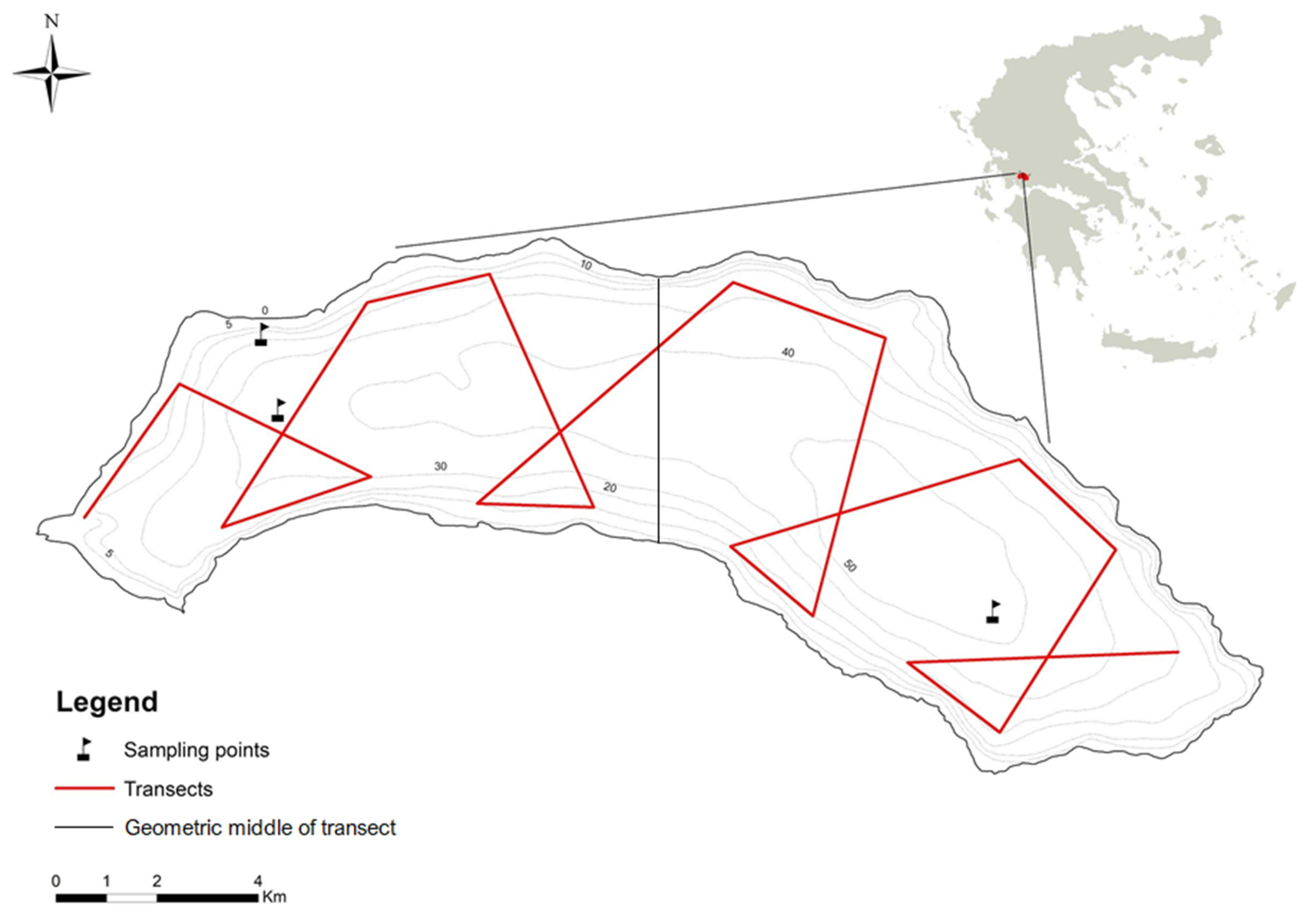
Equation (4) is valid for a temperature range of 10–40 °C [30], with a general reported maximum error of ~0.18 m/s (absolute value). Based on samplings at 3 locations (Figure 5), the temperatures recorded ranged from ~25 °C (surface layer) down to ~11 °C (hypolimnion). The 1-m depth interval recordings allowed the calculation of an overall standard deviation of the vertical distribution, which was equal to +/− 5.26, 4.77 and 4.35 °C for each station (in order of decreasing depth). The law of covariance propagation can be used to determine the standard deviation of sound velocity based on Equation (4):

σ²_c= (dc/dT)² × σ²_T = (4.624 − 0.0766 × T)² × σ²_T

(5)

Considering the average temperature of (25 + 11)/2 = 18 °C and the worst-case standard deviation of 5.26 °C, the sound velocity standard deviation is calculated as σ_c = ~17.07 m/s. The uncertainty propagation equation given in [27] for the depth error based on sound velocity variations is:

σ_zc² = (z/c)² × (σ_cm² + σ_c²)

(6)

In Equation (6), σ_cm accounts for sound velocity measurement variations and is considered to be compensated for through the instrument calibration procedure, i.e., is excluded from the equation. The σ_c parameter represents the spatiotemporal variations in sound velocity and corresponds to the value that was calculated above. Using this value and an average sound velocity based on the average temperature of 18 °C and Equation (4) equal to 1475.85 m/s, Equation (6) becomes:

σ_zc = (17.07/1475.85) × z = 0.011566 × z

(7)

For the worst-case depth of ~60 m, Equation (7) yields a depth error of ~0.69 m.

iii.

Time-Dependent Variations

The pulse length is an important determinant of the range resolution of transmission-based range measurement systems. According to Johannesson and Mitson [31], the physical length of the SONAR pulse in the water determines the vertical resolution between targets, i.e., provides the minimum separation distance between echoes. The pulse length is, therefore, also a determinant of the range accuracy, as it affects the minimum detectable height difference. This resolution can be calculated as half of the physical pulse length [31]:

dz_res = c × τ/2

(8)

Equation (8) corresponds to the average sound velocity in water, while τ represents the pulse duration. In this study, the pulse duration was set to 0.128 ms, and using the previously calculated average sound velocity of 1475.85 m/s the nominal vertical resolution is equal to σ_z(t) = ~0.094 m, regardless of the actual depth.

iv.

Water-Undulation-Related Variations

Variations due to the physical displacement of the device caused by natural undulations of the water surface also need to be accounted for [27]. Because the measurements were performed on windless days and with a moving vessel, pitch and heave were kept to a minimum. In order to estimate the effect of roll or heel (departure from the plumbline), this was calculated using the approximate vessel body geometry and the transect geometry along the trip, following appropriate adapted calculations of banked turns [32]. Approximating the turn radius along the trip as the local radius of curvature of the horizontal transect geometry, the minimum turn radius was determined to be ~130 m. Based on this value and using an approximate vessel body geometry and an average vessel travel velocity of 6 km/h, the worst case heel was calculated at ~0.18°, with an average value of 0.02° ± 0.03° along the transect. A worst-case divergence of ds = h × tan(0.18°) = ~0.003 × d (m) in the footprint is expected in the measurements. Given Equation (1), the ratio of (ds/R_{imprint-circle}) = tan(0.18°)/tan(3.5°) = ~0.05 in the worst case, i.e., ~5% over the total footprint, which is well within the spatial resolution of the produced raster (24 × 30 m), even for the largest depth values (e.g., ~18 cm for a worst-case footprint radius of 3.67 m). Furthermore, the worst-case effect introduced by this divergence on the vertical component of the measurements would be equal to 1/cos(0.18°) = 4.93 ppm, which is too small to produce a noticeable effect on the results.

Draft, settlement and squat all introduce a vertical displacement to the transducer, which is important to take into account with respect to the vertical accuracy of the measurements. In this study, the transducer was installed onto a bespoke supporting platform infrastructure providing suitable support for, and placed outside of, the boat. To compensate for the effects of draft, settlement and squat, the submersion level of the transducer was appropriately measured directly onto the transducer-supporting platform during the traversal, while the vessel was in full motion. Therefore, the sum of all effects was compensated for by adding the measured transducer submersion depth to all measurements.

Lake surface water level oscillation due to potential surface seiche effects was assessed using the empirically calculated maximum period of T = $2L/\sqrt{gh}$, where L is the bank-to-bank length, h is the average depth and g is the force of gravity [33,34]. Taking length values of ~19 km for the east–west bank distance and 5 km for the north–south bank distance, an average depth of 40.87 m and a value of 9.81 m/s² for the gravitational acceleration, the maximum east–west seiche period was calculated to be ~31.6 minutes for the east–west waves and ~8.3 min for the north–south waves. These periods constitute fractions of the total time of transect measurements (~4–5 h each), thus introducing a homogeneous distortion over the ensonified area of the lake, with areas of elevation and areas of depression with respect to the mean level being uniformly scattered in spatial terms. Additionally, the amplitude of those waves is expected to be very small on average, to the order of a few cm for moderately-sized lakes [34]. Therefore, it can be expected that those will be cancelled out in the statistical analyses, as the primary focus of this study is on the overall average accuracy of the studied data.

v.

Vertical Datum Error

In order to use the SONAR-acquired bathymetric measurements for absolute-scale comparisons, it is necessary to reduce the measured depths to an externally fixed vertical-reference system (vertical datum). In general, this error is not directly related to the echosounder instrument itself, but it indirectly affects the reliability (external precision) of the measurements.

• Overall Uncertainty

Considering a 2-sigma interval (95% confidence), thus replacing the σ of each relevant parameter with (2σ), the law of variance–covariance propagation was used to determine the bathymetric accuracy as a function of depth [27]:

$$\sqrt{{\sigma }_{z_m}^2+{\sigma }_{zc}^2+{\sigma }_{zt}^2}=\sqrt{0.000536z^2+0.035344}$$

(9)

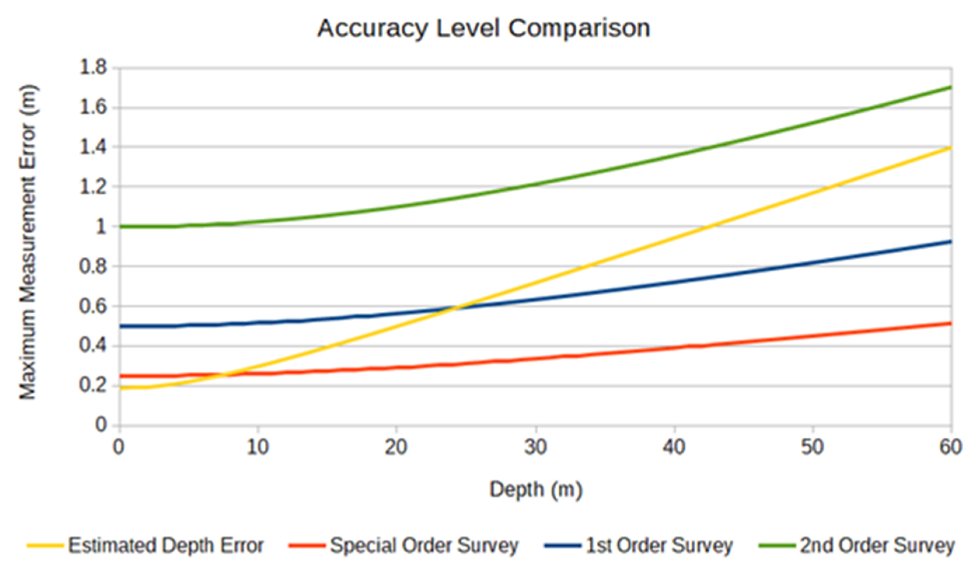
To assess the error budget, the S-44 requirements document was used [35]. The measurement accuracy estimation based on the conditions of this work, as described by Equation (9), was plotted against the corresponding requirements for a special order survey, as well as those for a 1st order survey. The results are shown in Figure 7. The estimated accuracy falls within the error margins of a 1st order survey (up to a depth of 24 m) and entirely within the error margins of a 2nd order survey (up to the maximum depth of 60 m). Additionally, the horizontal accuracy is entirely within the error margins of a 1st order survey (5 meters +/− 5% of depth) [35].

3.3.3. Data Processing

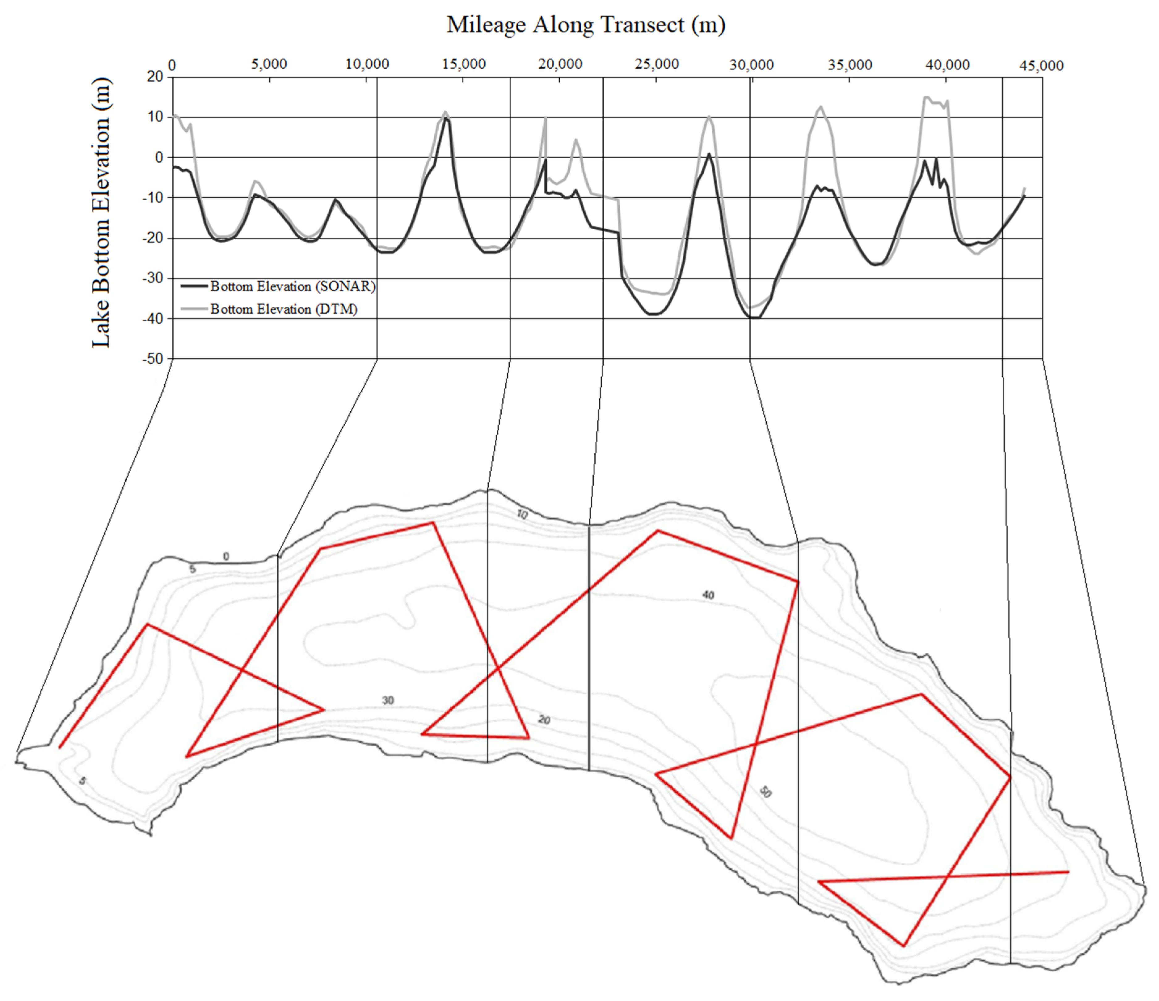
The collected hydroacoustic data were processed to obtain bathymetric information in the form of dense depth measurement points taken along the sampled transects. To ensure equally distributed weight among the evaluated DTM pixels and increased vertical accuracy, data measured multiple times over the same pixels were averaged.

The echosounder-derived bathymetric values were then converted into elevation (DTM) values by taking into account a suitable value for the mean water level of the lake. Information regarding the mean lake level at the time of the measurements was retrieved via the DAHITI (Database for Hydrological Time Series of Inland Waters) at the Lake Trichonis virtual station [36]. This information is acquired through appropriate processing of satellite altimetry data acquired from the Sentinel-3A satellite. The lake level data point from the DAHITI dataset for Lake Trichonis was characterized by a determination date difference of less than 2 days compared to the date of the echosounder measurements, with a value of 15.762 ± 0.013 m (7 October 2019). This value is in agreement with the latest regulation facilities constructed around Lake Trichonis. Specifically, the connecting canal between Lakes Trichonis and Lysimachia allows the regulation of the lake level from its old altitude of +18 m to altitudes ranging between 13.5 and 16.0 m. During the winter, large volumes of outflow are observed from Lake Trichonis while its level is significantly increased (by >1.5 m), which also results in an increased constant outflow towards Lake Lysimachia [19].

This lake level value of 15.762, which was used to reduce the bathymetric information to absolute elevations, is a normal height, in contrast to the DTM values, which are orthometric heights. However, because of the proximity of the area to the reference surface of the mean sea level (<50 m of absolute altitude), deviations between normal and orthometric heights are minimal [37] and well below the actual determination accuracy of the absolute altitude values themselves, both for the DTM and the echosounder measurements. Furthermore, large-scale studies (at the country and continent level) reveal a temporal variation of a few mm (generally <2 mm/year) in absolute geoid height as a long-term trend over the last few decades [38,39,40], whereas in Greece, average mean sea level variations slightly higher than that are also reported, e.g., 2.3 mm/year [41]. Therefore, the worst case total variation of ~16 cm for a timespan of 70 years is also insignificant with respect to the determination accuracy of the depth values, while the actual value is expected to be significantly smaller due to the existence, to some extent, of counter-balancing sub-periods in the last 70 years, as those are expected to cancel out a percentage of the total change magnitude. For all of the aforementioned reasons, no compensation was applied for those effects in the analyses.

The resulting dataset was subsequently used as the basis for the assessment of the DTM produced from the topographic maps, while the validation was performed at the relative and absolute levels, as well as in the form of a morphometric analysis.

3.4. Absolute Elevation Validation

To study the absolute elevation changes of the lake bottom between the DTM and SONAR datasets, descriptive statistics were calculated for the point-wise depth differences of the lake bottom, as measured and determined separately from the SONAR and the DTM. Using these differences, descriptive statistics were also calculated for the positive and negative values separately, along with the total transect lengths corresponding to these values.

More specifically, the depth of the DTM, d_DTM, was retrieved from the DTM model at each point, where the acoustic data depth, d_Acoustic, was also available. To perform a direct comparison, the difference between the vertical reference frames of the DTM and the echosounder-derived measurements, respectively, is assumed to have the form of a simple translation (displacement). Furthermore, this displacement is considered constant over the entire area of the lake. If d_DTM = h_{Lake_DTM} − h_{Bottom_DTM} and d_Acoustic = h_{Lake_Acoustic} − h_{Bottom_Acoustic} are the depth measurements at a single specific point i, then:

d_i = d_{i, Acoustic} − d_{i, DTM} = (h_{i, Lake_Acoustic} − h_{i, Bottom_Acoustic}) − (h_{i, Lake_DTM} − h_{i, Bottom_DTM})

(10)

Rearranging the terms results in:

d_i = d_i,Acoustic − d_{i, DTM} = (h_{i, Bottom_DTM} − h_{i, Bottom_Acoustic}) − (h_{i, Lake_DTM} − h_{i, Lake_Acoustic})

(11)

The (h_{Lake_DTM} − h_{Lake_Acoustic}) term of this equation represents the differences between the vertical reference frames of the old (DTM) and new (SONAR) dataset. For the sake of simplicity, this difference is assumed constant and independent of the measurement point over the lake area, denoted below as c. Therefore, the depth difference distribution is a translation of the actual distribution of the bottom height differences between the two epochs:

d_i = d_{i, Acoustic} − d_{i, DTM} = (h_{i, Bottom_DTM} − h_{i, Bottom_Acoustic}) + c

(12)

Using Equation (12), depth differences were calculated and mapped along the transect to study the distribution of the variations of the lake bottom terrain. The term c was calculated by using the available lake level values for the DTM and the SONAR measurements and used to calculate the mean elevation change of the lake bottom for further analysis.

3.5. Relative Elevation Validation

Contrary to any absolute error estimation, the relative bathymetry validation process is independent of changes to the lake water level. Hence, any relative errors may be attributed to the inaccuracies of the bathymetric model, but may also reflect changes of the topography of the lake bottom surface, for example due to sedimentation or tectonic processes.

The relative height difference between points i and j is expressed as:

d_ij = (d_{j, Acoustic} − d_{i, Acoustic}) − (d_{j, DTM} − d_{i, DTM}) = (d_{j, Acoustic} − d_{j, DTM}) − (d_{i, Acoustic} − d_{i, DTM}) = d_j − d_i

(13)

Replacing Equation (12) and rearranging it leads to:

d_ij = (h_{j, Bottom_DTM} − h_{i, Bottom_DTM}) − (h_{j, Bottom_Acoustic} − h_{i, Bottom_Acoustic}) = dh_{ij, DTM} − dh_{ij, Acoustic}

(14)

To estimate the relative bathymetric accuracy, a random selection of 3284 differences—between an equivalent number of 3284 available samples drawn as averages over the matching pixels—was carried out. The relative accuracy was then assessed on the basis of these computed depth differences using Equation (14).

3.6. Bathymetric Model

Apart from the descriptive statistics for the absolute point-wise depth differences between the two datasets, a parametric model was also fit to study the variations after the absorption of potential systematic differences and outliers, which may be due to various sources, ranging from variations of the corresponding vertical reference frames up to distortions introduced by the HMGS map sheet digitization procedure. In the absence of information regarding the accuracy of the bathymetry extraction techniques and measurements followed by the HMGS, it is assumed that classic sparse depth measurement techniques were used, such as the sinking of ropes or rods up to the bottom of the lake.

The bathymetric model serves as a diagnostic tool for the DEM’s assessment. The statistical results of the fitting surface provide a sense of the consistency between the DEM and the SONAR depths, respectively. While the model coefficients mainly absorb the systematic differences (e.g., inclinations, different datum realizations), the descriptive statistics of the residuals (minimum, maximum, mean and standard deviation) quantify the agreement between the different depth computation sources. Large residuals would, therefore, indicate accordingly large inconsistencies.

To validate the accuracy of the DTM derived from the digitized map sheets, a 2nd degree polynomial was applied:

$$\delta d_i=d_i^{SONAR}-d_i^{DTM}=a_0+a_1{\phi }_i^2+a_2{\lambda }_i^2+a_3{\phi }_i{\lambda }_i+a_4{\phi }_i+a_5{\lambda }_i+e_i,$$

(15)

where $d_i^{SONAR}$ is the acoustically derived depth and $d_i^{DTM}$ is the DTM-derived depth (from the HMGS) at point i, whereas φ and λ represent the WGS84 geodetic latitude and longitude of the points, a_i represent the unknown model parameters and e_i represents the residual of the observed depth difference between the two datasets. This model corresponds to a common 2nd order corrector surface model from the general polynomial model family. The specific choice was based on a generic attempt to fit polynomials from the 1st up to the 3rd degree, accordingly, with the 2nd degree being found to provide optimal fit statistics.

Prior to application, the observed differences were filtered for outliers using the widely applied 3-sigma rejection criterion (thus rejecting observations with |δd_i| > 3 × σ). The estimation of the unknown parameters and the residuals was carried out using a least-squares fit of (15), the descriptive statistics of the fit were calculated and their histogram and cumulative distribution were appropriately charted. Using the resulting model, the relative residuals were also calculated as:

$$\mathsf{\Delta }\delta d_{ij}=\delta d_j-\delta d_i,$$

(16)

which is effectively a reformulation of Equation (14). The analysis was performed for all possible relative residual pairs (after outlier removal) and the histogram and cumulative distribution function were also charted in this case.

3.7. Morphometric Analysis

The morphometric characteristics of the elevation variation between the DTM and the echosounder-derived lake bottom data were studied as further analyses of the absolute and relative depth differences based on Equations (12) and (14), respectively. The main aim of these analyses was to facilitate inference with respect to sources of bottom elevation variations (e.g., mass redistribution, inflow or both), and generally the spatial characteristics of processes that have potentially affected the surface morphology of the lake bottom, as well as its volume, in the time period between the production of the two compared datasets (DTM vs. SONAR measurements).

Since the acoustic transect expands primarily in the east–west direction, the approximate geometric “middle” of the lake was considered at ~20 km of the transect length and descriptive statistics were calculated for the east and west parts of the lake based on the corresponding transect parts (first vs. second approximate half). Apart from this, correlation analyses were performed between bottom elevation differences and geographic position (latitude and longitude), distance from the shore, as well as absolute bottom elevation (based on the DTM). To study the effect of potential changes on the overall water volume, the area under the curve was calculated for the DTM-derived and SONAR-derived depth profiles as proxies and the values were compared.

Spatial trends in the depth difference distribution were also researched through local 3D surface fitting in order to capture potential sloping behaviors. To this end, point coordinates were projected to a locally tangent Cartesian plane with the help of an azimuthal equidistant projection and a 1st order polynomial surface model (plane) was fitted using least-squares estimation between the bottom elevation difference values (Equation (12)) and the mean-center-reduced projected coordinates of the measurement points (x’ = x − x_average, y’ = y − y_average):

d_i = a₀ + (a₁ · x′) + (a₂ · y′)

(17)

The use of horizontal coordinates for this analysis was preferred in order to obtain a result that can be readily interpreted in 3D space, with respect to a plane that is locally tangential to the ellipsoid. Additionally, to more appropriately serve a geological point of view, Tukey’s fences [42] were used for outlier detection as a more robust method (due to the asymmetry of the distribution), while maintaining, however, a higher tolerance to outliers (k = 3, instead of the typical value of 1.5) in order to include a higher percentage of potentially important signals. To study the variations in morphological characteristics of the DTM in time, the relative height differences of Equation (14) were also interpreted as indicators of shape variation of the lake bottom surface. Since those height differences eliminate the effect of the external vertical frame of reference, the comparison technically yields a measure of the observed change in intrinsic morphology, i.e., the co-variation between each pair of points i and j. Because the following analyses were based on a subset of point pairs, bootstrapping was employed to increase the robustness of the results. Therefore, all subsequent analyses were performed for 30 random subsets of 5000 point pairs each and the results are presented as averages, accompanied by their standard deviations.

To study the variations in corresponding point pairs, and thus in the overall shape relief, correlation analysis was performed between the DTM and echosounder-derived bathymetric point pair elevation differences. To assess the significance of the variations in light of the determined echosounder accuracy, a Student’s paired t-test was performed with the null hypothesis that the relative depth difference distributions would be equal between the produced DTM and the echosounder-based measurement derivation at the 95% confidence level (a = 0.05):

$$H_0:d_{ij}=0\iff dh{~}_{ij,Acoustic}=dh{~}_{ij,DEM}$$

(18)

The accuracy of the differences calculated by Equation (14), necessary for the assessment of hypothesis (19), depends on both the accuracy of the produced DTM and the accuracy of the echosounder-derived dataset, combined appropriately as (based on covariance propagation):

$${\sigma }_{d_{ij}}^2={\sigma }_{d{h}_{ij,Acoustic}}^2+{\sigma }_{d{h}_{ij,DEM}}^2,$$

(19)

where ${\sigma }_{d{h}_{ij,DEM}}^2$ represents the accuracy of the depth difference as calculated from the DTM and ${\sigma }_{d{h}_{ij,Acoustic}}^2$ represents the accuracy of the depth difference as calculated from the echosounder-derived data.

The accuracy of the acoustic bathymetric data was analytically derived as a function of the measured depth at both points of each pair using Equation (9), while the accuracy was propagated to derive the final accuracy of the height difference. In the absence of information regarding the accuracy of the produced DTM, it is impossible to determine the total inaccuracy of each determined d_ij value. However, one of the primary aims of this study was to look for potential morphological changes with respect to the bathymetry, as it is represented by the DTM itself. Therefore, the depth values of the produced DTM are considered to be the known parametric values in the above analysis, such that ${\sigma }_{d{h}_{ij,DEM}}^2=0$, and only the echosounder-derived measurements are examined under the hypothesis:

Under the aforementioned assumption, the values of Equation (19) were acquired for each pair and the corresponding t-statistic values were calculated at the a = 0.05 (1.96 − sigma) level. These values were plotted in increasing order and each one was separately compared to $t_{df}^{1-\frac{a}{2}}=t_{\infty }^{0.975}=1.96$ to evaluate the significance of the difference. The percentage of significant differences was finally calculated and reported for the bootstrapped samples.

4. Results

4.1. DTM

The DTM from the available cartographic information was referenced to WGS84 and mapped using a depth gradient and bathymetric contour lines, yielding the final output (Figure 8).

4.2. Absolute Elevation Error

The distribution of differences between bathymetric values from the produced DTM and the corresponding values derived from the acoustic data were plotted in the form of a histogram (Figure 9), while the corresponding descriptive statistics were also calculated (

Table 2. Descriptive and other statistics of the bathymetric model errors (h_DTM − h_SONAR).

Statistical Measure	Value
Mean (m)	3.39
Standard Deviation (m)	5.26
RMSE (Root Mean Squared Error) (m)	5.38
RMSE 95% (m)	3.90
RMSE 90% (m)	2.98
Median (m)	1.51
NMAD (Normalized Median Absolute Deviation) (m)	2.86
(Excess) Kurtosis	2.48
Skewness	–1.71
Minimum (m)	–3.93
Maximum (m)	24.05
Range (m)	27.98
N (number of samples)	3284

). Each class label in Figure 9 indicates the upper limit of the corresponding 1 m interval. Most values were classified in the interval of [1–2) m, while the distribution is asymmetric, leaning far more towards the negative side, meaning that the SONAR-derived depths are generally higher than the corresponding values of the DTM within the measured subset. The elevation differences, as well as the absolute bottom elevation values for both datasets, were also plotted along the measured transect to study their spatial distribution across the lake (Figure 10 and Figure 11).

The average lake bottom elevation difference (h_DTM − h_SONAR) is equal to 3.39 ± 5.26 m, which indicates a noteworthy (with respect to the external effects described in the methodology section) displacement between the two datasets (Figure 11). Approximately 82.5% of the data points fall within the 1-sigma range (|dh_SONAR-DTM − 3.39| < 5.26 m), while ~17.5% of the data points are 1-sigma outliers. In the 1-sigma range subgroup, the average bottom elevation difference is 1.67 ± 2.3 m, whereas in the outlier subgroup, the average bottom elevation difference is 11.49 ± 7.31 m.

The average lake bottom elevation from the DTM data is equal to −13.719 ± 13.1 m, whereas the average lake bottom elevation from the SONAR data is equal to −17.044 ± 10.15 m, indicating a lower overall dispersion in the SONAR dataset. The total length along the transect, where h_DTM − h_SONAR > 0, was equal to ~32 km, with an average elevation difference value equal to 4.77 ± 5.29 m. The total length along the transect, where h_DTM − h_SONAR < 0, was equal to ~12 km, with an average elevation difference value equal to 1.03 ± 0.86 m. These values indicate that the distribution of the morphological changes over the lake transect are not uniform, but ~27% of the current bottom elevation along the SONAR transect (12 km out of a total of 44 km of transect length) actually lies above its older (DTM) level (positive average), and is in fact rather smooth (as indicated by the relatively smaller standard deviation).

Considering a transect mileage value of ~20 km as the separating line between the east and west parts of the lake (Figure 10 and Figure 11), the average bottom elevation difference for the west part of the lake (first half of transect) is equal to −1.72 ± 3.24 m, whereas the corresponding value for the east part of the lake is equal to −4.638 ± 6.08 m (second half of measured transect). Therefore, the east part of the lake appears to have been affected almost 3 times as much as the west part (see also Figure 19) by the apparent elevation changes over the studied time period, while the range of variations has almost doubled.

Analysis of the absolute elevation difference versus distance of the transect segments from the shore revealed only a weak trend (R² = 0.09, p = 0.2, Figure 12). However, the same analysis performed at the subgroup of elevation difference outliers at the 1-sigma level (|dh_SONAR-DTM − 3.39| < 5.26 m) indicated a relatively stronger correlation with distance from the shore (R² = 0.31, p = 0.01, Figure 13). The correlation analysis for the latitude–longitude distribution of the elevation difference did not reveal any significant trends at the alpha = 0.05 significance level (R² < 0.1, p > 0.05). A strong (R² = 0.74, p = 1.2 ∙ 10⁻³⁸, d = 0.013 × h²_DTM + 0.563 × h_DTM + 6.314) 2nd degree polynomial-based correlation and also a relatively strong positive linear correlation (R² = 0.49, p = 8.2 × 10⁻¹⁵, d = 0.278 × h_DTM + 7.145) were detected between lake bottom elevation difference (h_DTM − h_SONAR) and absolute lake bottom elevation based on the DTM model (Figure 14). This result indicates that the magnitude of the bottom differences between the ~1950 and 2019 datasets increases as lake bottom elevations increase for the DTM elevation dataset. Since absolute elevation is also an indicator of depth (considering a constant-altitude lake water level surface), this indicates that higher discrepancies generally occur at smaller depths.

4.3. Relative Elevation Error

The distribution of relative difference residuals between the produced DTM and the acoustically derived data were also plotted as a histogram (Figure 15) and descriptive statistics were calculated (

Table 3. Descriptive and other statistics for the relative bathymetric model errors.

Statistical Measure	Value
Mean (m)	0.00
Standard Deviation (m)	7.49
RMSE (Root Mean Square Error) (m)	7.49
RMSE 95% (m)	6.20
RMSE 90% (m)	5.22
Median (m)	0.72
Normalised Median Average Deviation (NMAD) (m)	2.86
(Excess) Kurtosis	1.17
Skewness	0.04
Minimum (m)	–24.80
Maximum (m)	24.67
Range (m)	49.47
n (number of samples)	3284

). The distribution appears to be much closer to normal with a larger overall dispersion, as signified by the total range of almost 50 m and standard deviation of 7.24 m.

4.4. Bathymetric Model

After rejecting 354 absolute depth differences and based on Equation (15), a bathymetric model corrector surface was fitted to 2931 absolute depth residuals, leading to the following fit statistics (

Table 4. Descriptive statistics for 2nd order bathymetric corrector surface fit.

Mean	0.00 m
Median	–0.09 m
Minimum	–6.30 m
Maximum	4.60 m
Standard Deviation	2.11 m

):

The statistics are also visualized in Figure 16 and Figure 17. It is important to stress that the 3-sigma outliers excluded from this analysis represented 354 out of 3284 observations, i.e., almost 11% of the total. While this amount is not entirely unexpected, in light of the asymmetry and overall characteristics of the original distribution (Figure 9, Table 2), this exclusion is only a statistical necessity that aids in minimizing distortions and achieving a best fit for the two surfaces. It is necessary to keep in mind that the excluded values may represent an observed signal that is meaningful, e.g., from a geological, geomorphological or tectonic point of view.

In order to study the intrinsic consistency of the bathymetric correction model, a relative residual analysis was also performed based on Equation (16). After the exclusion of outliers, descriptive statistics were calculated from a total of 4,293,915 relative depth differences (

Table 5. Descriptive statistics for relative residuals of 2nd order bathymetric corrector surface fit.

Mean	0.29 m
Median	0.18 m
Minimum	−10.42 m
Maximum	10.89 m
Standard Deviation	2.81 m

, Figure 18 and Figure 19).

A bias (mean) of 0.29 m is noted from the relative residual analysis, while the standard deviation is not strikingly different to that of the absolute residual analysis. The total range of values for the relative residuals reveals significant differences in the morphologies of the DTM and the SONAR datasets. This can be attributed to the erroneous nature of the HMGS bathymetric observations, while it is also possible that some outliers may have gone undetected due to the limited suitability of the 3-sigma outlier detection technique for distributions that deviate significantly from the norm (e.g., asymmetric), as in the case of the present analysis.

4.5. Morphometry

4.5.1. Absolute Depth and Volume

Interpreting the depth measurements from the produced DTM, as well as from the SONAR, as the distance between the lake water surface and the corresponding bottom, the area under each transect depth–mileage profile (Figure 20) was calculated and compared between the two datasets. This area can be used as a proxy for the water volume and the bottom morphology along the transect. Notably, the total area under the curve was found to be equal to 1,463,795 m² (~1.46 km²) for the SONAR-derived profile (2019), while a value of 1,413,329 m² (~1.41 km²) was calculated for the DTM-derived profile (~1950). This indicates a slightly higher water volume along the transect (with the SONAR-derived profile being ~1.0357 times larger) between the two datasets.

For the fitting of a plane surface, all points were projected to a plane that was locally tangential to the ellipsoid and their coordinates were reduced to the local mean center (x_c, y_c) to minimize distortion, truncation errors and other numerical artifacts, while a total of 89 outliers (~2.7%) were rejected based on Tukey’s fences with k = 3.0 (thus excluding only extreme outliers farther than 3 interquartile ranges from the lower and upper quartiles, respectively).

Table 6. Results and statistics for surface fits for (h_DTM − h_SONAR).

	1st Order Surface (Plane)
Coefficient of (x’)	0.0003035
Coefficient of (y’)	0.0004229
Constant Term	2.913 m
Mean Error	0.000 m
Median Error	–0.931 m
Minimum	–6.645 m
Maximum	16.689 m
Range	23.334 m
Mean Absolute Error	3.148 m
RMSE	4.331 m

and Figure 21 depict the fit statistics and the distribution of the errors of the model. The wider range and the apparent asymmetry in the distribution are inherited from the original elevation difference distribution and indicate the preservation of the (potentially significant) effects of marginal signals on the result.

Apart from its potential interpretation as a corrector surface, this 1st order surface also provides an intuitive indication of the magnitude of change (slope) of the depth difference between the DTM values and the SONAR measurements in the east–west and north–south directions, outwards from the mean center of the measured point dataset. The results indicate a rate of change equal to 0.0003035 in the east–west direction, which is equivalent to a ~30 cm/km increase in the h_DTM − h_SONAR component, whereas in the north–south direction, the elevation difference rate of change for the same component is equal to 0.0004229, or ~42 cm/km. These values indicate a trend of NE-oriented increase in the (h_DTM − h_SONAR) component, and therefore a larger discrepancy between bottom elevations, with DTM values generally being larger than SONAR values. This can be viewed as a gradual NE-directed “subsidence” of the SONAR-measured lake bottom with respect to the produced DTM. The main direction of this apparent subsidence vector based on the determined components is oriented at an azimuth approximately equal to 35.668°. Additionally, the results indicate an average elevation decrease of ~2.913 m since the production of the map sheets that the DTM creation was based on (Table 6).

4.5.2. Relative Depth

Depth differences from the DTM (dh_ij,DTM) compared to depth differences from the SONAR-derived dataset (dh_ij,acoustic) for the same point pairs i-j (Equation (14) were correlated on a bootstrapping basis of 30 iterations with 5000 pairs. Figure 22 depicts the outcome of one of these instances, however the coefficient of determination and the coefficients of the equation displayed are averages accompanied by their corresponding standard deviations, as acquired from all 30 iterations. Specifically, the final regression coefficients for the equation dh_ij,DTM = a ∙ dh_ij,acoustic + b were calculated to be a = 1.1996 ± 0.0078, b = 0.0083 ± 0.0093 and the coefficient of determination was calculated to be equal to R² = 0.8662 ± 0.00339 (Figure 22).

Paired t-tests performed between the two distributions for a total of 30 random selections of 5000 point pairs indicated that p < 0.05 less than 0.5% of the time (i.e., p < 0.05 occurred for only 1 out of 30 random iterations). Based on the t-tests, the two datasets (DTM vs. SONAR) were found to have the same average value for the measured subset of the lake at the 95% confidence level, which was also validated by the fact that the confidence interval for coefficient b contains the value of zero at alpha = 0.05. Apart from that, since b can be considered practically equal to 0, the regression coefficient a ≈ 1.2 can practically be interpreted as a scale factor, i.e., (dh_ij,DTM/dh_ij,acoustic = a). As a result, a systematic difference in the intrinsic scale (i.e., not in absolute but in relative terms) is also apparent between the two datasets, with DTM depth differences being, on average, 1.2 times larger in absolute terms than the corresponding SONAR depth differences for the same point pairs.

For one of the instances of 5000 randomly selected point pairs, the t-statistic was calculated for each double-difference value and the sorted value distribution was plotted (Figure 23). Regardless of specific instance depicted, the figure also displays the average percentage and the standard deviation of the values that are below the critical value of $t_{\infty }^{0.975}$ = 1.96 (average and standard deviation acquired from 30 iterations). Based on the calculations, approximately 20.25% ± 0.5% of the analyzed point pairs were not detected as statistically significant changes in depth difference between the pair points. Conversely, in approximately 80% of the measured subset, a significant intrinsic morphological change is detected at the 95% confidence level. This observation demonstrates a potential intrinsic morphological change of a magnitude that the SONAR-based measurement accuracy is adequately capable of detecting at the 95% confidence level, having occurred at approximately 80% of the measured part of the lake bottom. This change corresponds to the detected systematic morphological change of the lake bottom surface from the previous analysis, as indicated by the detected intrinsic scale difference factor of 1.2 between the DTM and SONAR models.

5. Discussion

The basis of the overall DTM assessment for Lake Trichonis consisted of (a) the DTM interpolation method used for the production, i.e., the Topo-to-Raster algorithm, (b) the estimated SONAR measurement accuracy, (c) the absolute and relative elevation validation, (d) the subsequent bathymetric model and (e) the estimation of the magnitude of morphological changes. Taking into account the measured water level decrease of more than 2 m (from 18 m in ~1950 to ~15.76 in 2019), the results indicate ground deformation of the lake bottom, as well as potential overall subsidence. The Topo-to-Raster interpolation error of ±0.4 m and its spatial distribution, together with the acoustic measurement estimated average accuracy of about ±0.7 m (maximum of 1.4 m only at the maximum lake depth), indicate that the identified lake bottom elevation changes of more than 3 m between ~1950 and 2019 are not spurious, but well within the cumulative overall accuracy and determination capabilities of the derived data and employed analysis methods. The signal-to-noise ratio approximation, calculated as the ratio of the interpolated DTM depth to interpolation error, also indicates the overall relatively small influence of the interpolation error on the extracted DTM depths along the transect.

Regardless of the drop in water level, the measurements indicate that the total water volume (estimated through the depth profile transect area under the curve as a proxy) has not been affected, even exhibiting a slight (approximately 1.04 times in terms of transect surface) increase in 2019 compared to ~1950. The water level decrease and the fact that the lake volume does not decrease substantially despite increased water pumping for various purposes, such as irrigation or residual overflow into Lake Lysimachia, have been documented in the past [16,19]. Psilovikos et al. [19] reported significant amounts of water being discharged into the lake, especially in its eastern karst area, by underground and underwater springs. These springs effectively contribute to recycling the total water volume of the lake in excess to the otherwise seemingly inadequate amount of precipitation alone.

The generally observed subsidence trend between ~1950 and 2019 is confirmed by previous research recognizing the Trichonis basin as a pull-apart basin generally undergoing a sinking process with time [43]. The intense seismicity of the surrounding area is well documented [44,45,46], with general ground deformation rates to the order of ~10 mm/year [43,47]. Lake Trichonis is located in the vicinity of the Amfilochia–Katouna–Aitoliko Fault Zone, which is a recognized subsiding basin [48] with extensive underground karstic networks from water-facilitated limestone corrosion and solution [49]. Historical satellite observation dataset analysis (ERS1/2) indicates an effect of ~5.5.mm/year of subsidence in the west part of the lake [50], which is approximately half that of the values reported for the rest of the lake, explaining the observed difference in subsidence magnitudes in this study. Furthermore, karst landscapes are generally known to be prone to subsidence, depending on the stage of hydrogeological evolution [51]. However, the cumulative effect and order of magnitude of the aforementioned subsidence factors does not suffice to explain the observed overall displacement of >3 meters over 50 years. One explanation for this inconsistency could be attributed to sudden irregular subsidence events outside of typical long-term, gradual, pull-apart basin dynamics.

Notably, Kiratzi et al. [48] point out a concentration of epicenters in the vicinity of the SE area of the lake, with a notable strong earthquake event sequence taking place in 1975 (Mw: 5.6 on 30 June 1975 and Mw: 6.0 on 31 December 1975), with the 31 December event even producing landslide events [49,52]. In this study, a 1st degree surface fit between depth differences was found to indicate a NE-oriented increase in the h_DTM − h_SONAR component, which expresses absolute bottom subsidence. This demonstrates a generally increasing observed lake bottom subsidence in the NE direction, with a maximum descent direction azimuth of ~35.668°. This direction of maximum descent in relatively reasonable accordance to the NE dip direction of ~46° north (strike angle equal to ~316°) of a NW–SE normal fault was determined to have been the mechanism for the 1975 earthquake event documented by Kiratzi et al. [48], with a dip angle equal to ~71°. In addition, a similar mechanism of a NNW–SSE strike fault zone that also dips in the NE direction was determined to have been ruptured during the April 2007 earthquake swarm (average Mw of 5.2) in the proximity of the lake, while epicenters were found to cluster along the eastern part of the lake shore, following a NNW–ESE distribution trend [48]. The dip direction of this normal fault is also close to the determined azimuth value of 35.67° for the direction of the maximum lake bottom descent of this study, while the focused intense seismic activity at the east part of the lake in 1975 and 2007 might explain the larger observed subsidence in the east part of the lake.

The analysis with respect to the distance from the shore led to mixed results. Because of the morphology of the lake, deeper parts generally have larger distances from the shore. However, while differences in lake bottom elevation between ~1950 (DTM) and 2019 (SONAR) do not exhibit a correlation to distance from the shore, difference values outside the 1-sigma confidence interval (i.e., |d| > ~5.2 m, which is the overall standard deviation of the difference values along the transect) exhibit a more significant correlation (R² = 0.51), with signed values decreasing with increasing depth. This decrease in the h_SONAR – h_DTM component indicates a decreasing trend in bottom depth in 2019 compared to ~1950, which is more intense in deeper areas. Because of the karstic network underlying the lake [19], this observation can be attributed in part to the effect of the larger hydrostatic pressure, and hence the larger water column mass, applied to the lake bottom at deeper areas, as pressure increases linearly with depth (p – p₀ = ρ·g·h). This result can be contrasted to the result in Figure 14, which effectively indicates that at an elevation level of approximately −21.65 m (global minimum of the 2nd degree polynomial curve), the lake bottom exhibits the lowest overall differences between the two datasets along the overall transect. A possible reason for this could be the steepness of those areas (the contour density around the ~20 m depth contour is higher, Figure 8), meaning that they might not be retaining significant amounts of matter, as the latter could flow towards deeper, flatter areas. In addition, the subsidence at those relatively steeper areas is slightly less affected by the hydrostatic pressure force, due to the deviation of the surface normal from the plumbline (because of the steepness), thus resulting in a slightly smaller overall vertical subsidence component.

Analysis with respect to relative depths and bottom elevations was performed to investigate the morphological changes of the lake bottom, as well as the reliability of the results. Considering the analyzed measurement accuracy of the echosounder-derived dataset at each point, statistically significant differences were determined at approximately 80% of the total measured data. This indicates an intrinsic morphological deformation in an adequate order of magnitude, which is detectable with the specific SONAR. Correlation analysis revealed a potential scale difference between altitude differences, with no apparent displacement coefficient. More specifically, the lake bottom relief was approximately 1.2 times more exaggerated in terms of bottom altitude differences in the DTM dataset compared to the echosounder-derived dataset. This can be interpreted as a smoothening of the measured subset of the lake bottom, which is in agreement with the aforementioned geological effects, as a consequence of the water-flow mediated lake bottom erosion, combined with relief homogenization through subsidence, potentially owing in part to the karstic nature of the lake underground. The scale difference of 1.2 could in part be attributed to systematic errors in the derivation of the DTM (1950) dataset. A constant difference would not be possible to determine in this analysis, as differences would eliminate such an effect. However, the intrinsic scale difference could be attributed to a corresponding systematic scale distortion of the instruments used in the 1950 data acquisition campaigns. Generally, while impossible to totally exclude this possibility, attributing the entire effect exclusively to the instruments used would not be realistic, given the large timespan between the two datasets.

As a last note, it also ought to be mentioned that in the past, cases of dynamite use for fishing have been reported (personal communication with local people) to a varying extent. This practice usually takes place in shallower waters and this seems to correlate well with the observed higher elevation differences closer to the shore (in higher bottom elevations). It is important to highlight that this practice would have also had unspecifiable nontrivial effects on the surface of the lake bottom, which may have played a role in the overall differences observed between the DTM (~1950) and SONAR (2019) datasets.

6. Conclusions

The present study was concerned with the evaluation of a digital terrain model from existing topographic mapping data sources of Lake Trichonis, using recent bathymetric information acquired through the processing of hydroacoustic and GPS data. A DTM was successfully produced through interpolation of topographic and bathymetric information obtained from digitized maps provided by the HMGS, dating back to the year ~1950. Hydroacoustic data were collected along a transect covering the area of the lake in a coil-shaped pattern and were converted to bathymetric information using appropriate processing steps. With the help of satellite altimetry data providing a high-accuracy value for the lake water level, the hydroacoustically derived bathymetric data were converted to absolute elevation values for the lake bottom, referencing the year 2019 (and more specifically the beginning of October). The two sources of lake bottom elevation (SONAR vs. DTM) were compared along the measured transect to evaluate the accuracy and validity of the ~1950 DTM for the lake bottom.

The results indicate substantial discrepancies between the old DTM and contemporary acoustic data. These may generally reflect intrinsic or extrinsic changes of the lake bottom topography, owing to subsidence, sedimentation, karstic or geodynamic or tectonic phenomena. In the case of Lake Trichonis, the significant deviations of the 2019 bathymetric dataset with respect to the ~1950 lake DTM and overall morphometry appear to be associated with a combination of tectonics, subsidence and karstic phenomena in the area. On the contrary, an effect of accumulated sediment deposition was not detectable on the basis of the DTM validation, as the overall water volume has remained practically unchanged. These observations could prove useful in terms of the tectonics, geodynamics and seismicity with respect to the broader Corinth Rift region, as well as for environmental management and technical interventions in and around the lake. Nevertheless, it is also important to highlight the value of a new, complete dataset for validation purposes, following the updated topographic mapping of the lake bottom and bathymetry instead of targeted SONAR measurements, which inevitably only cover a fraction of the total lake area. Such a dataset would dictate the necessity for new, extensive bathymetric measurements in order to produce an updated DTM of Lake Trichonis, reflecting current conditions and tailored to contemporary accuracy standards to the order of a few cm, as well as state-of-the-art research in various disciplines in and around the lake.

References

1. Messager, M.L.; Lehner, B.; Grill, G.; Nedeva, I.; Schmitt, O. Estimating the volume and age of water stored in global lakes using a geo-statistical approach. Nat. Commun. 2016, 7, 1–11. [Google Scholar] [CrossRef]
2. Søndergaard, M.; Jeppesen, E. Anthropogenic impacts on lake and stream ecosystems, and approaches to restoration. J. Appl. Ecol. 2007, 44, 1089–1094. [Google Scholar] [CrossRef]
3. Shanahan, T.M.; Overpeck, J.T.; Sharp, W.E.; Scholz, C.A.; Arko, J.A. Simulating the response of a closed-basin lake to recent climate changes in tropical West Africa (Lake Bosumtwi, Ghana). Hydrol. Process. Int. J. 2007, 21, 1678–1691. [Google Scholar] [CrossRef]
4. Quinn, N.W.; Hanna, W.M. A decision support system for adaptive real-time management of seasonal wetlands in California. Environ. Model. Softw. 2003, 18, 503–511. [Google Scholar] [CrossRef] [Green Version]
5. Håkanson, L. The importance of lake morphometry and catchment characteristics in limnology–ranking based on statistical analyses. Hydrobiologia 2005, 541, 117–137. [Google Scholar] [CrossRef]
6. Popielarczyk, D.; Templin, T.; Łopata, M. Using the geodetic and hydroacoustic measurements to investigate the bathymetric and morphometric parameters of Lake Hancza (Poland). Open Geosci. 2015, 7, 1–16. [Google Scholar]
7. Li, Z.; Zhu, Q.; Gold, C. Digital Terrain Modeling: Principles and Methodology; CRC Press: Boca Raton, FL, USA, 2005. [Google Scholar]
8. Yuzugullu, O.; Aksoy, A. Generation of the bathymetry of a eutrophic shallow lake using WorldView-2 imagery. J. Hydroinform. 2014, 16, 50–59. [Google Scholar] [CrossRef]
9. Abdallah, H.; Bailly, J.S.; Baghdadi, N.N.; Geours, S.N.; Fabre, F. Potential of space-borne LiDAR sensors for global bathymetry in coastal and inland waters. IEEE J. Sel. Top. Appl. Earth Obs. Remote Sens. 2012, 6, 202–216. [Google Scholar] [CrossRef] [Green Version]
10. Bandini, F.; Olesen, D.H.; Jakobsen, J.; Kittel, C.M.M.; Wang, S.; Garcia, M.; Gottwein, B.P. Bathymetry observations of inland water bodies using a tethered single-beam sonar controlled by an unmanned aerial vehicle. Hydrol. Earth Syst. Sci. 2018, 22, 4165–4181. [Google Scholar] [CrossRef] [Green Version]
11. Arseni, M.; Roșu, A.; Georgescu, L.P.; Murariu, G. Single beam acoustic depth measurement techniques and bathymetric mapping for Catusa lake Galati. Ann. Univ. Dunarea Jos Galati Fascicle II Math. Phys. Theor. Mech. 2016, 39, 281–287. [Google Scholar]
12. Holcombe, T.L.; Youngblut, S.; Slowey, N. Geological structure of Charity Shoal crater, Lake Ontario, revealed by multibeam bathymetry. Geo-Mar. Lett. 2013, 33, 245–252. [Google Scholar] [CrossRef]
13. Popielarczyk, D.; Templin, T. Application of integrated GNSS/hydroacoustic measurements and GIS geodatabase models for bottom analysis of Lake Hancza: The deepest inland reservoir in Poland. Pure Appl. Geophys. 2014, 171, 997–1011. [Google Scholar] [CrossRef] [Green Version]
14. De Moustier, C.; Matsumoto, H. Seafloor acoustic remote sensing with multibeam echo-sounders and bathymetric sidescan sonar systems. Mar. Geophys. Res. 1993, 15, 27–42. [Google Scholar] [CrossRef] [Green Version]
15. Dost, R.J.J.; Mannaerts, C.M.M. Generation of lake bathymetry using sonar, satellite imagery and GIS. In Proceedings of the ESRI International User Conference GIS, Geography in Action, San Diego, CA, USA, 4–8 August 2008. [Google Scholar]
16. Dimitriou, E.; Moussoulis, E. Hydrological and nitrogen distributed catchment modeling to assess the impact of future climate change at Trichonis Lake, western Greece. Hydrogeol. J. 2010, 18, 441–454. [Google Scholar] [CrossRef]
17. Tafas, T.; Danielidis, D.; Overbeck, J.; Amilli, E.A. Limnological survey of the warm monomictic lake Trichonis (central western Greece); I. The physical and chemical environment. Hydrobiologia 1997, 344, 129–139. [Google Scholar] [CrossRef]
18. Zacharias, I.; Dimitriou, E.; Koussouris, T. Integrated water management scenarios for wetland protection: Application in Trichonis Lake. Environ. Model. Softw. 2005, 20, 177–185. [Google Scholar] [CrossRef]
19. Psilovikos, A.; Albanakis, K.; Palikaridis, C.; Vouvalidis, K. Enironmental value and importance of Lake Trichonis as the largest natural freshwater reservoir of Greece. In Proceedings of the 4th Panhellenic Geographical Conference, Athens, Greece, 12–14 October 1995; pp. 348–358. (In Greek). [Google Scholar]
20. HMGS. The Basic Cartographic Scale. Hellenic Military Geographical Service. (In Greek). Available online: https://drive.google.com/file/d/1PZJpAFOZaiqgZp-aBGoaAWqspMDoS9z6/view (accessed on 4 October 2020).
21. Monmonier, M. The History of Cartography, Volume 6: Cartography in the Twentieth Century, 1st ed.; University of Chicago Press: Chicago, IL, USA, 2015; Volume 6. [Google Scholar]
22. Böhme, R.; Anson, R. Inventory of World Topographic Mapping Volume 3–Eastern Europe, Asia, Oceania and Antarctica. International Cartographic Association; Elsevier Applied Science: Amsterdam, The Netherlands, 1989; Volume 3. [Google Scholar]
23. ESRI. How Topo to Raster Works. Available online: https://pro.arcgis.com/en/pro-app/latest/tool-reference/3d-analyst/how-topo-to-raster-works.htm (accessed on 31 January 2021).
24. Wahba, G. Spline Models for Observational Data; Society for Industrial and Applied Mathematics: Philadelphia, PA, USA, 1990. [Google Scholar]
25. Hengl, T. Finding the right pixel size. Comput. Geosci. 2006, 32, 1283–1298. [Google Scholar] [CrossRef]
26. Perivolioti, T.M.; Frouzova, J.; Tušer, M.; Bobori, D. Assessing the Fish Stock Status in Lake Trichonis: A Hydroacoustic Approach. Water 2020, 12, 1823. [Google Scholar] [CrossRef]
27. IHO. Depth Determination. In Manual on Hydrography (Publication C-13), 1st ed.; International Hydrographic Bureau: Monaco, France, 2005; p. 539. [Google Scholar]
28. Tušer, M.; Balk, H.; Mrkvička, T.; Frouzová, J.; Čech, M.; Muška, M.; Kubečka, J. Validation of current acoustic dead-zone estimation methods inlakes with strongly sloped bottoms. Limnol. Oceanogr. Methods 2011, 9, 507–514. [Google Scholar]
29. Chen, C.T.; Millero, F.J. The use and misuse of pure water PVT properties for lake waters. Nature 1977, 266, 707–708. [Google Scholar] [CrossRef]
30. Lubbers, J.; Graaff, R. A simple and accurate formula for the sound velocity in water. Ultrasound Med. Biol. 1998, 24, 1065–1068. [Google Scholar] [CrossRef]
31. Johannesson, K.A.; Mitson, R.B. Fisheries Acoustics: A Practical Manual for Aquatic Biomass Estimation. FAO Fisheries Technical Paper 240; Technical Paper; Food and Agriculture Organization of the United Nations: Rome, Italy, 1983. [Google Scholar]
32. Barrass, C.B.; Derrett, D.R. Heel Due to Turning. In Ship Stability for Masters and Mates, 7th ed.; Butterworth-Heinemann, Elsevier: Massachusetts, MA, USA, 2012; pp. 145–147. [Google Scholar]
33. Mühll, K.V.D. Über die Bewegung tropfbarer Flüssigkeiten in Gefässen. Nach Johann Rudolf Merian. Math. Ann. 1886, 27, 575–600. [Google Scholar]
34. Kalff, J. Limnology: Inland Water Ecosystems; Prentice Hall: Upper Saddle River, NJ, USA, 2002. [Google Scholar]
35. IHO. IHO Standards for Hydrographic Surveys (Special Publication No S-44), 6th ed.; International Hydrographic Organization: Monaco, France, 2020. [Google Scholar]
36. Schwatke, C.; Dettmering, D.; Bosch, W.; Seitz, F. DAHITI-An innovative approach for estimating water level time series over inland waters using multi-mission satellite altimetry. Hydrol. Earth Syst. Sci. 2015, 19, 4345–4364. [Google Scholar] [CrossRef] [Green Version]
37. Sjöberg, L.E. A refined conversion from normal height to orthometric height. Studia Geophys. Geod. 2006, 50, 595–606. [Google Scholar] [CrossRef]
38. Glowka, K.G.; Krynski, J.; Szelachowska, M. Time variations of the gravity field over Europe obtained from GRACE data. Rep. Geod. Geoinform. 2012, 92, 175–190. [Google Scholar]
39. Godah, W.; Szelachowska, M.; Krynski, J. On the analysis of temporal geoid height variations obtained from GRACE-based GGMs over the area of Poland. Acta Geophys. 2017, 65, 713–725. [Google Scholar] [CrossRef] [Green Version]
40. Wu, F.; Zeng, A.; Ming, F. Analyzing the long-term changes in China’s National Height Datum. Adv. Space Res. 2020, 66, 1342–1350. [Google Scholar] [CrossRef]
41. Bitharis, S.; Ampatzidis, D.; Pikridas, C.; Fotiou, A.; Rossikopoulos, D.; Schuh, H. The Role of GNSS Vertical Velocities to Correct Estimates of Sea Level Rise from Tide Gauge Measurements in Greece. Mar. Geod. 2017, 40, 297–314. [Google Scholar] [CrossRef]
42. Tukey, J.W. Exploratory Data Analysis, 1st ed.; Pearson: London, UK, 1977. [Google Scholar]
43. Vassilakis, E.; Royden, L.; Papanikolaou, D. Kinematic links between subduction along the Hellenic trench and extension in the Gulf of Corinth, Greece: A multidisciplinary analysis. Earth Planet. Sci. Lett. 2011, 303, 108–120. [Google Scholar] [CrossRef]
44. Armijo, R.; Meyer, B.; King, G.; Rigo, A.; Papanastassiou, D. Quaternary evolution of the Corinth Rift and its implications for the Late Cenozoic evolution of the Aegean. Geophys. J. Int. 1996, 126, 11–53. [Google Scholar] [CrossRef] [Green Version]
45. Briole, P.; Rigo, A.; Caen, L.H.; Ruegg, J.C.; Papazissi, K.; Mitsakaki, C.; Balodimou, A.; Veis, G.; Hatzfeld, D.; Deschamps, A. Active deformation of the Corinth rift, Greece: Results from repeated Global Positioning System surveys between 1990 and 1995. J. Geophys. Res. 2000, 105, 605–625. [Google Scholar] [CrossRef] [Green Version]
46. Papazachos, B.C.; Papazachos, C.B. The Earthquakes of Greece, 3rd ed.; Ziti Publications: Thessaloniki, Greece, 2003. (In Greek) [Google Scholar]
47. Benekos, G.; Parcharidis, I.; Foumelis, M.; Ganas, A. Ground deformation measurements over Lake Trichonis based on SAR interferometry. Bull. Geol. Soc. Greece 2013, 47, 1071–1080. [Google Scholar] [CrossRef] [Green Version]
48. Kiratzi, A.; Sokos, E.; Ganas, A.; Tselentis, A.; Benetatos, C.; Roumelioti, Z.; Serpetsidaki, A.; Andriopoulos, G.; Galanis, O.; Petrou, P. The April 2007 earthquake swarm near Lake Trichonis and implications for active tectonics in western Greece. Tectonophysics 2008, 452, 51–65. [Google Scholar] [CrossRef]
49. Delibasis, N.; Carydis, P. Recent earthquake activity in Trichonis region and its tectonic significance. INGV Ann. Geophys. 1977, 30, 19–81. [Google Scholar]
50. Psychogyiou, C.; Papoutsis, I.; Kontoes, C.; Poyiadji, E.; Spanou, N.; Klimis, N. Multi-temporal monitoring of slow-moving landslides in South Pindus mountain range, Greece. In Proceedings of the Fringe 2015 Workshop, Frascati, Italy, 23–27 March 2015. [Google Scholar]
51. Klimchouk, A.B. Subsidence hazards in different types of karst: Evolutionary and speleogenetic approach. Environ. Geol. 2005, 48, 287–295. [Google Scholar] [CrossRef] [Green Version]
52. Papadopoulos, G.A.; Plessa, A. Magnitude–distance relations for earthquake-induced landslides in Greece. Eng. Geol. 2000, 58, 377–386. [Google Scholar] [CrossRef]
Figure 1. Location of the study area.
Ijgi 10 00091 g001
Figure 2. Available topographic and bathymetric information of the broader study area from 1:50,000 scaled maps (HMGS).
Ijgi 10 00091 g002
Figure 3. Estimation and spatial distribution of the Topo-to-Raster algorithm interpolation error.
Ijgi 10 00091 g003
Figure 4. Transect-wise plot of the interpolated depth to interpolation error ratio. Axis Y shown in logarithmic scale.
Ijgi 10 00091 g004
Figure 5. Echosounding traverses and sampling point locations for temperature measurements.
Ijgi 10 00091 g005
Figure 6. Supporting infrastructure for the acquisition of GPS and hydroacoustic measurements.
Ijgi 10 00091 g006
Figure 7. Overall survey accuracy vs. IHO (International Hydrographic Organization) Document S-44 accuracy requirements plot.
Ijgi 10 00091 g007
Figure 8. The final bathymetric model at a resolution of 1″ × 1″ produced from the available digitized HMGS map sheets by interpolation of the relevant topographic and bathymetric information.
Ijgi 10 00091 g008
Figure 9. Histogram and cumulative distribution of (hDTMhSONAR) values.
Ijgi 10 00091 g009
Figure 10. Absolute lake bottom elevation variation along the measured transect (with spatial reference) as derived from the DTM and the SONAR dataset.
Ijgi 10 00091 g010
Figure 11. Absolute lake bottom elevation differences (hDTMhSONAR) along the lake transect (with spatial reference).
Ijgi 10 00091 g011
Figure 12. Elevation difference (hDTMhSONAR) vs. distance from the shore—correlation analysis plot.
Ijgi 10 00091 g012
Figure 13. Elevation difference (hDTMhSONAR) vs. distance from the shore—correlation analysis plot for the 1-sigma outlier subgroup (data points with absolute elevation differences > 5.2 m).
Ijgi 10 00091 g013
Figure 14. Correlation analysis between elevation differences and lake bottom elevation based on the DTM dataset with 2nd order polynomial fit.
Ijgi 10 00091 g014
Figure 15. Histogram of relative bathymetric model errors.
Ijgi 10 00091 g015
Figure 16. The histogram of the residuals of the 2nd order model after the fit to the absolute residuals.
Ijgi 10 00091 g016
Figure 17. The empirical and theoretical cumulative distribution functions (CDFs) of the results.
Ijgi 10 00091 g017
Figure 18. The histogram of the relative residuals calculated based on the 2nd order surface fit.
Ijgi 10 00091 g018
Figure 19. The empirical and theoretical cumulative distribution functions of the results.
Ijgi 10 00091 g019
Figure 20. Measured depth comparison between SONAR and DTM along transect.
Ijgi 10 00091 g020
Figure 21. Histogram and cumulative distribution of the 1st order (plane) surface fit errors for the (hDTMhSONAR) component.
Ijgi 10 00091 g021
Figure 22. Relative depth differences compared between DTM- and acoustic-data-derived bathymetry.
Ijgi 10 00091 g022
Figure 23. Sorted distribution of t-statistic values produced from point pair differences (dhij,DTMdhij,acoustic) along with estimated standard deviations. The line indicates the critical t-value (df → ∞, a = 0.05).
Ijgi 10 00091 g023