Machine Learning Methods Applied to the Prediction of Pseudo-nitzschia spp. Blooms in the Galician Rias Baixas (NW Spain)

Abstract

This work presents new prediction models based on recent developments in machine learning methods, such as Random Forest (RF) and AdaBoost, and compares them with more classical approaches, i.e., support vector machines (SVMs) and neural networks (NNs). The models predict Pseudo-nitzschia spp. blooms in the Galician Rias Baixas. This work builds on a previous study by the authors (doi.org/10.1016/j.pocean.2014.03.003) but uses an extended database (from 2002 to 2012) and new algorithms. Our results show that RF and AdaBoost provide better prediction results compared to SVMs and NNs, as they show improved performance metrics and a better balance between sensitivity and specificity. Classical machine learning approaches show higher sensitivities, but at a cost of lower specificity and higher percentages of false alarms (lower precision). These results seem to indicate a greater adaptation of new algorithms (RF and AdaBoost) to unbalanced datasets. Our models could be operationally implemented to establish a short-term prediction system.

1. Introduction

Harmful algae blooms (HABs) are an increasingly frequent and intense event in coastal areas worldwide [1,2]. HABs affect the ecosystem and human health and impact on fish and aquaculture activities and regional economies [3].

The detection and monitoring of HABs is traditionally based on field samplings [3,4]. Recently, increasing attention has been paid to the development of prediction models, which could aid in the early warning of blooms and improve the effectiveness of management programs. The prediction of phytoplankton blooms includes the application of several methods which can vary in modelling approach and complexity [5].

Conventionally, the prediction of harmful algal events is based on statistical numerical models, such as logistic regression, regression trees or Bayesian models [6,7,8,9,10]. However, most of these approaches are limited to linear systems, while HABs usually occur in complex and highly dynamic coastal environments [11,12].

Machine learning models have been used due to their capability to deal with complex, often non-linear and noisy datasets and to generate predictive models of relatively high accuracy [13,14,15,16].

Support vector machines (SVMs) were first described in 1992 [17] and later developed for classification and regression [18,19]. Briefly, SVMs are a linear classifier operating in a higher dimensional feature space using kernel functions. SVMs search for the optimal hyperplane by maximizing the margin using the Lagrange method to solve a quadratic optimization problem constrained by linear restrictions [20]. SVMs have achieved good results in different applications related to the detection of blooms of different types of algae in both freshwater [15,21,22,23,24,25] and coastal [16,20,26,27,28,29] environments.

Neural networks (NNs) are widely used in environmental applications due to their ability to model multivariate, complex and non-linear data [30]. Theoretical foundations of NNs were introduced by McCulloch and Pitts in the 1940s [31]. A multilayer perceptron (MLP) NN is composed by a set of nonlinear computational elements (neurons or nodes) arranged in multiple layers that are interconnected in a feedforward way with each connection defined by a weight value. It usually includes an input layer, one or more hidden layers and an output layer. While the input layer distributes the input signals into the network, neurons in the hidden and output layers process their input signals using an activation function. MLPs are trained by a back-propagation learning procedure which adjusts iteratively the weight values in order to minimize an error function [30]. NNs have been extensively applied to HABs prediction, especially in fresh-water systems [15,23,32,33,34]. In coastal waters, NN models have been developed for predicting blooms of specific HAB species [16,28,29,35,36,37,38] or estimating in advance the chlorophyll-a concentration, which is often used as a proxy for phytoplankton abundance [39,40].

Random Forest (RF) was initially created by Tin Kam Ho applying random decision trees. Breiman and Cutler extended these random decision trees by introducing the bootstrap aggregation (or bagging) technique [41]. RF is an ensemble machine learning algorithm which consists of multiple decision trees working in parallel, so that the final output is defined using a “voting” system. In case of binary classification (bloom/no bloom), the final result is the most “popular” class, i.e., the output for the majority of trees [41]. RF has been extensively used in ecological modelling [42,43,44], and during the last years, it has been successfully employed to HAB prediction [15,26,28,45,46,47,48].

Boosting is a machine learning technique based on combining a set of weak classifiers to create a high-performance prediction rule. AdaBoost (Adaptative Boosting), introduced by [49], is one of the most widely used boosting algorithms. AdaBoost combines single-node decision trees named stumps, in series: once a tree is trained, the subsequent tree tries to correct the errors in the previous one, by adapting the weights associated with each tree in order to take the final decision. AdaBoost has been recently applied to different ecological applications [50,51], while few works are also focused on microalgae [16,26,52].

All abovementioned approaches use a set of parameters as input data, regardless of the modelling technique. Common environmental predictors include water temperature and salinity, chlorophyll-a concentrations, nutrients or meteorological parameters, such as wind or rainfall (see review in [14,15]). Some authors also consider lagged abundance of species in previous weeks [20,37], or integrate satellite imagery into the bloom prediction [28,53]. Prediction approaches also define different outputs such as phytoplankton abundance [16,21,23,24,32,33,34,35,36,37,38], toxin concentration [22,46], and chlorophyll-a concentration as indicator of phytoplankton biomass [25,32,39,40] or binary outputs, i.e., no bloom/bloom [20,27,28] or absence/presence [28,47].

Some approaches combine machine learning models with other techniques. For instance, SVMs were integrated with particle swarm optimization [22,24] or MLPs were improved using a genetic algorithm to search for the optimal initial parameters [29]. Bourel et al. [26] propose different consensus methods combining results from different machine learning binary classifiers (including boosting, SVM and RF) for predicting presence/absence of different phytoplankton species.

Some studies show comparative results using different machine techniques. For example, Yu et al. [16] found that gradient boosted descent tree achieves a better performance as compared to other methods such as SVM, NN or AdaBoost. Ribeiro and Torgo [23] reported that SVM provides better accuracy than regression trees or NN predicting algae blooms in the Douro River (Portugal). The consensus method showed the best accuracy for most of the phytoplankton datasets analyzed by [26]. The latter also obtained good results using boosting, SVM and specially RF. In the approach based on remote sensing data developed by [28], long short-term memory recurrent NN showed better results than MLP, RF or SVM. Results by [29] in Tolo Harbour (Hong Kong) indicated that MLP outperforms SVM or generalized regression neural networks.

In view of these results, there is not an unequivocal “best” machine learning method for HABs prediction, and the development of an adequate approach is dependent on the target species, the region and the characteristics of the available dataset.

This study focuses on the HABs caused by Pseudo-nitzschia spp. in the Rias Baixas area in Galicia (NW Spain). Several species of the genus Pseudo-nitzschia such as Pseudo-nitzschia multiseries and Pseudo-nitzschia australis have been associated with the production of the neuro-toxin domoic acid (DA), which causes amnesic shellfish poisoning (ASP) toxicity [54,55]. This genus is generally common in upwelling systems, for example, in the California Current System [56], in the Iberian System [20,57,58] and the Benguela area [59].

Few works have addressed the prediction of Pseudo-nitzschia spp. blooms on coastal areas. Blum et al. [60] developed multiple linear regression models to predict DA level using data from culture and natural blooms in Cardigan Bay (Canada). Stepwise linear and logistic regression models were developed to predict both DA and Pseudo-nitzschia spp. abundance in the Santa Barbara Channel [61], Monterey Bay [8] and Chesapeake Bay [6]. A mechanistic model was proposed by [62] to simulate the DA production. Empirical approaches based on the prediction of favorable conditions for the development of blooms of Pseudo-nitzschia spp. were explored for the Lisbon Bay [58] or the Galician coast [63]. Cusack et al. [64] forecasted the onset, abundance and duration of Pseudo-nitzschia blooms in the southwest coastal waters of Ireland using a zero-inflated negative binomial model. The application of particle tracking models to simulate the short-term dynamics of Pseudo-nitzschia spp. events have been proposed for southwest Ireland [65] and the north-west Pacific [66]. Townhill et al. [67] have projected the future distribution of Pseudo-nitzschia spp. and other species in the north-west European shelf using the maximum entropy MaxEnt model. Absence/presence and abundance short-term forecast models based on NNs and using biological and environmental 20-years long time-series from Alfacs Bay (NW Mediterranean) were developed by [36].

This study builds on previous work developed by [20], in which absence/presence and no bloom/bloom Pseudo-nitzschia spp. SVM models were developed for the Galician Rias Baixas using a long-term dataset (1992–2001) of environmental parameters. For no bloom/bloom models, one of the main issues is the imbalance of the dataset, with only around 15% of samples identified as bloom. Consequently, models with a good sensitivity tend to show a higher rate of false alarms. Therefore, the main aim is to explore the potential of different machine learning methods to find a better balance between sensitivity and precision and improve the results found by [20]. In addition to the most extended machine learning technologies for HABs prediction (SVM and NN), we introduce recent ensemble learning methods (RF and AdaBoost), which are expected to show a better generalization ability by combining multiple weak learners [16].

In summary, we present a comparison of different machine learning approaches, i.e., MLP, SVM, RF and AdaBoost, to predict blooms of Pseudo-nitzschia spp. in the Rias Baixas. Models were developed and validated using a long-term weekly dataset (2002–2012) of environmental parameters using the same approach and dataset structure (combinations of variables) proposed by [20].

2. Materials and Methods

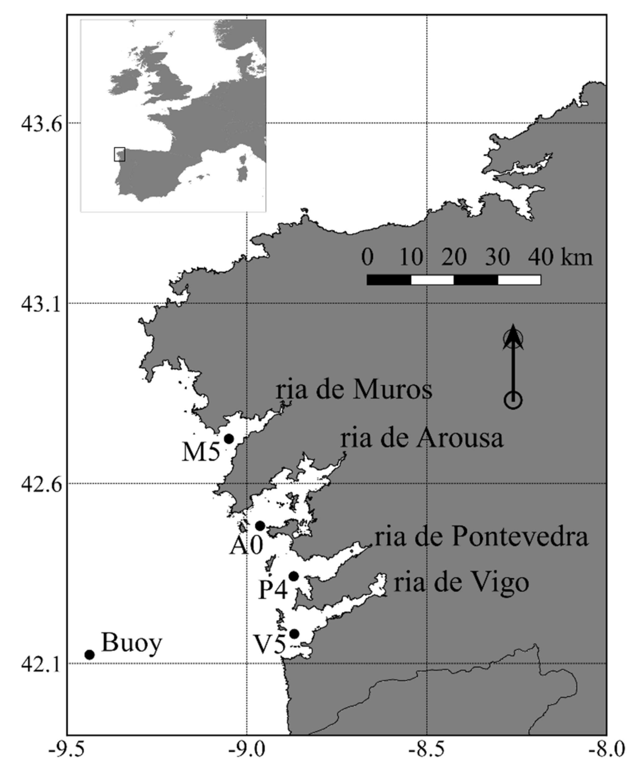
2.1. Study Area

A ria (rias in plural) is a Spanish name for the V-shape coastal embayments located on the west coast of Galicia (NW Spain), which were formed by the partial submergence of ancient river valleys. The Rias Baixas are the four southern rias, from south to north: Vigo, Pontevedra, Arousa and Muros (see Figure 1). They are located along the northern boundary of the NW African upwelling system [68]. In this region, the seasonality of the ocean dynamics is governed by the relative strengths and latitudinal shifts of the Azores high-pressure and the Iceland low-pressure systems. Wind-driven processes in the area generate strong upwelling of rich nutrient cold waters in the period from May to September (these waters rise up to the photic zone, reaching the surface in the more intense upwelling) [69,70], leading to significant increases in primary production (up to 7.4 g C m⁻² d⁻¹) during upwelling events [71].

This area supports an intensive mollusk (mainly mussels) culture using floating rafts. Galicia is the region with the highest production of aquaculture mussels in Europe and one of the world leaders. Mussel production in this area reaches approximately 250,000 t per year, equivalent to 41% of the European production and 15% of the world production [72].

These activities are seriously hindered by harmful algae blooms (HABs), which cause an important ecological, social and economic impact since they can even force the closure of production areas [73,74]. HABs are a frequent and well-documented phenomenon in Galicia, and a great number of studies can be found in the literature since the 1950s [75,76,77,78]. One of the main HAB-forming taxonomic groups is Pseudo-nitzschia spp., which has been detected since 1994 as the causative agent of ASP toxic events due to the production of domoic acid (DA) [79,80,81].

Due to the economic importance of aquaculture, a monitoring program of HAB species was set up in Galician waters. The Technological Institute for the Control of the Marine Environment of Galicia (INTECMAR) conducts a weekly routine sampling, measuring the abundance of Pseudo-nitzschia spp. (and other potentially toxic species), water quality parameters and biotoxin levels in mussels and other mollusks [20].

Prediction in advance of HABs is very important for mollusk producers in terms of organization and logistics, as well as for the social policies related to one of the main economic driving forces in the region [20,80,81].

2.2. Dataset

The dataset used in this study includes weekly records of water parameters (i.e., temperature, salinity and Pseudo-nitzschia spp. abundance) and upwelling indices between January 2002 and December 2012. We used the same dataset structure and variables presented in [20].

Water parameters (i.e., temperature, salinity, Pseudo-nitzschia spp. abundance) were measured by INTECMAR as part of its monitoring program consisting of a weekly sampling at 38 sampling stations distributed across the four Rias Baixas. We only considered data from the outer stations located at the mouth of each ria (Figure 1; V5 in the ria of Vigo, P4 in the ria of Pontevedra, A0 in the ria of Arousa and M5 in the ria of Muros). These stations are not affected by local processes (e.g., river discharges) and are considered to be representative of the open ocean conditions.

Temperature and salinity measurements were collected in situ from the surface to 5 m depth, approximately every 10 cm, using a Seabird Model 25 CTD. Specifically, temperature was measured using a Seabird SB3 thermistor (range: −5° to +35 °C; precision: 0.02 °C; resolution: 0.0003 °C) and salinity is based on a Sea Bird SBE4 conductivity cell (range: 0–7 S/m; precision: 0.0003 S/m; resolution: 0.00004 S/m). Temperature and salinity values for each week and station were then computed by integrating all the available valid measurements using the trapezoidal rule.

Regarding phytoplankton, samples were collected using tow nets (10 µm mesh) from the surface to 15 meters depth, fixed with formaldehyde 4% and stored under dark and cool conditions. Total abundances (in cells L⁻¹) of Pseudo-nitzschia spp. and other potential toxic taxonomic groups were counted using an inverted light microscope at 250× and 400× magnification [82].

As proposed by [20], five upwelling indices (Iw), one for the sampling day and four for each one of the four previous days, were estimated from wind data measured at Cape Silleiro oceanographic buoy (42.12°N, 9.43°W, see Figure 1). This buoy, moored at a depth of 323 m, is a SeaWatch buoy of Puertos del Estado (http://www.puertos.es, accessed on 20 January 2021) equipped with meteorological instruments to measure wind speed (range: 0–60 m/s; accuracy: ±0.3 m/s) and direction (range: 0 to 360°; accuracy: ±3°) at 10 m above sea level every ten minutes. Winds at this location are considered representative of wind conditions in the Galician area [83].

Upwelling indices were computed using the Bakun’s method [84]:

Iw = (−τ_y)/(ρ_w·f) = (−1000·ρ_a·C_D ·W·W_y)/(ρ_w·f) m³/(s · km)

(1)

In the equation above, τ_y is the meridional component of the wind force (N m⁻²), ρ_w is the density of seawater (1025 kg m⁻³), f is the factor of Coriolis (9.9 × 10⁻⁵ s⁻¹ at 42° de latitude), ρ_a is the density of the air (1.2 kg m⁻³ at 15 °C), C_D is a dimensional empirical drag coefficient (1.4 × 10⁻³), and W and W_y are the daily average of the wind speed and its meridional component, respectively. Positive upwelling indices indicate upwelling conditions (dominant northerly winds, negative W_y values) while negative indices are related to downwelling situations (dominant southerly winds, positive W_y values).

We established two categories based on Pseudo-nitzschia spp. abundance to define the output of the models: no bloom (<10⁵ cell L⁻¹) and bloom (≥10⁵ cell L⁻¹) [20]. We also defined as input variables the ria code (1: Arousa; 2: Muros; 3: Pontevedra; 4: Vigo), the day of the year (between 1 and 366), and the occurrence of a bloom in the previous week (bloom-1w) or two previous weeks (bloom-2w) using a value between 0 and 15 indicating in which rias the bloom was detected (0: no bloom; 1–4: bloom in one ria; 5–10; bloom in two rias; 11–14: bloom in three rias; 15: all rias) [20].

Variables are summarized in

Table 1. List of variables included in the models, indicating the number of records and valid records, as well as the minimum and maximum values used to scale each variable.

Variable (Units)	#Records	#Valid Records	Min. Scale	Max. Scale
Temperature (°C)	2065	2054	10	20
Salinity (psu)	2065	1976	24	36
Upwelling indices (m3s−1km−1) (Day -4 to Day 0)	4015	4015	−2500	2500
Pseudo-nitzschia spp. abundance (cell/L)	2153	2153
Day of the year			1	366
Ria code			1	4
bloom-1w, bloom-2w			1	15

. Note that water parameters (temperature, salinity, Pseudo-nitzschia spp. abundance) were not available every week due to two reasons: (1) there was no field sampling campaign because of bad weather or ship breakdown; (2) sampling problems, such as erroneous readings, instruments failures or excessive detritus. The number of valid records for these variables is also shown in Table 1.

Models were developed using the same combination of variables proposed by [20] and labelled using letters from A to D: A includes all the available variables; B excludes the spatial and temporal effects (ria code and day of the year); C also discards information about bloom occurrence in previous weeks (bloom-1w, bloom-2w) and D is only based on upwelling indices. A dataset was built for each combination by associating the input variables with the corresponding output (bloom or no bloom) for each day and ria, removing records with invalid or missing values for any of the input or output variables. The variables and number of records available for each combination are shown in

Table 2. Combinations of variables used to develop the models, and total number of records available for each combination.

Combination	Variables	#Records
A	day of the year; ria code; temperature; salinity; bloom-1w; bloom-2w; upwelling indices.	1829
B	temperature; salinity; bloom-1w; bloom-2w; upwelling indices.	1829
C	temperature; salinity; upwelling indices	1831
D	upwelling indices	1920

.

After removing invalid and missing values, final datasets include between 79.66% (combination A or B) and 83.62% (combination B) of 2296 potential records (i.e., 574 weeks × 4 stations).

2.3. Model Selection

We divided the complete dataset for each combination of features (A, B, C or D) into two independent datasets, the training (2/3 of the total records) and validation sets (1/3 of the records). Both subsets were built including a similar percentage of both classes (bloom and no bloom). Models were developed (i.e., trained) using the training set, while the validation set was useful for obtaining an independent set of performance measurements to select the optimal model.

Table 3. Number of records available for de training and validation of the models for each combination of features (A, B, C or D, see Table 2).

	Training Set			Validation Set
	Total	No Bloom	Bloom	Total	No Bloom	Bloom
A	1220	1027	193	609	508	101
B	1220	1025	195	609	510	99
C	1221	1022	199	610	515	95
D	1280	1070	210	640	549	91

summarized the number of records included in each dataset for both classes.

In the case of the SVM and NN, input data were linearly scaled to a range between −1 and +1 before training in order to avoid a greater influence of variables with larger numeric ranges [85]. Categorical features (bloom occurrence in previous weeks and ria code) were firstly converted into numeric data. Table 1 shows the minimum and maximum values used to scale these variables.

The optimal parametric configuration for each combination of features and method was selected by a hyperparameter optimization. This was based on a grid search approach, i.e., models using different parameters controlling the learning process are trained and evaluated, and the best models are selected according two metrics (F1-score and distance to point (0,1) in the operating receiver characteristics (ROC) curve, see Section 2.3). The metrics were computed using the validation set. Selected hyperparameters and swept values are shown in Section 2.4. All the experiments were carried out using the libraries available in MATLAB with the exception of NNs, which were also programmed in Matlab but using a custom code. The code is available in a GitHub repository: https://github.com/currobellas/NeuralNetwork (accessed on 20 January 2021).

2.4. Performance Measurements

The models’ performance was evaluated by comparing the results with the real output through a confusion matrix [86], a 2 × 2 table showing the number of samples correctly classified for both classes (no bloom and bloom), as well as the number of false positives and false negatives.

Different metrics extracted from the confusion matrix are proposed in the literature. In this work, we considered the sensitivity and the specificity, i.e., the percentage of bloom and no bloom records correctly classified, respectively; and the precision, fraction of true positives with respect to the total number of records classified as bloom. Regarding global metrics, global accuracy (percentage of records correctly classified) could provide misleading information because of the unequal distribution of classes (around 16% of bloom, 84% of no bloom). Hence, we used the F1-score, defined as the harmonic mean of precision and sensitivity, which is widely used with imbalanced datasets [87].

In order to compare models graphically, we also built operating receiver characteristics (ROC) curves plotting the sensitivity against the false positive rate (1—specificity) and computed the distance to the optimal point (0,1) (i.e., all the bloom records are correctly classified at this point) as a metric combining sensitivity and specificity [88,89].

Although confusion matrixes were built from the training and validation subsets, results from the validation set are expected to be more reliable since this subset is not included in the training process. Therefore, optimal models were selected according to two criteria based on metrics computed from the validation set: maximum F1-score and minimum distance to the optimal point (0,1) in the ROC curve. All the metrics shown in this work are based on the validation results.

2.5. Machine Learning Methods

2.5.1. Support Vector Machines (SVM)

In this work, in addition to the Gaussian radial basis (RBF) kernel chosen by [20], we tested polynomials kernels of various degrees (until 50) for each combination of features (A, B, C or D).

2.5.2. Multilayer Perceptron (MLP)

For each combination of features (A, B, C and D), we performed 660 tests varying the following settings:

• Number of hidden layers in the neural network: from 1 to 10.
• Number of iterations in the backpropagation algorithm: 50, 100, 500, 1000, 1500 and 2000.
• Lambda regularization factor: 0.00001, 0.00005, 0.0001, 0.0005, 0.001, 0.005, 0.01, 0.05, 0.1, 0.5, and 1.

2.5.3. Random Forest (RF)

We employed the following parameters to unravel the optimal parametric configuration for each combination of variables (A, B, C or D):

• Number of bags for bootstrapping: 30, 40, 50, 60, 70, 80, 100, 200, 300, 400, 500 and 1000.
• Number of weak predictors selected as subset for each tree: between 2 and 4.

Note that a weak predictor is considered as a variable to make a decision, and hence the number of weak predictors has to be lower than the total number of input variables.

2.5.4. AdaBoost

We have combined two parameters for searching the optimal model for each combination of features (A, B, C or D):

• Type of boosting variant: GentleBoost, AdaBoostM1 and RUSBoost.
• Number of cycles (parameter directly related to the number of weak classifiers): 10, 50, 100, 150, 200, 500, 1000 and 2000.

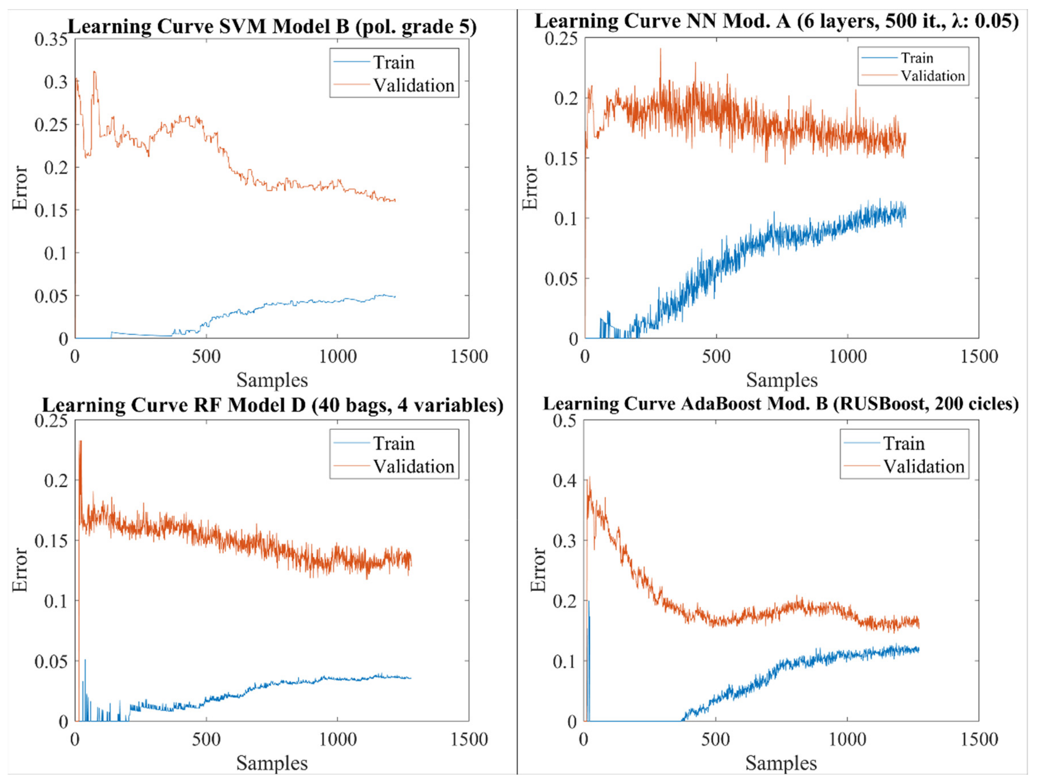
2.6. Learning Curves

Learning curves were obtained by plotting the training and validation errors against the number of samples used in the training process [90]. Training error is expected to be low when the samples number is low, but it will increase as new samples are included in the training process. The validation error is expected to decrease with an increasing number of training samples. These curves are useful for analyzing the trade-off between bias and variance errors.

If a model shows a good fitting to the training set but fails to fit the validation set, there is a problem of variance or overfitting. In the learning curve, as the number of samples increases, the training error remains low, but the validation error is high. In this case, the model could be improved by increasing the number of training samples.

However, if both training and validation errors are similar but with high values, there is a problem of bias or underfitting. In the learning curves, as the number of samples increases, both error curves tend to touch themselves. In this case, increasing the number of samples would not reduce the error and the model could be improved by adding new variables.

3. Results

3.1. Observations

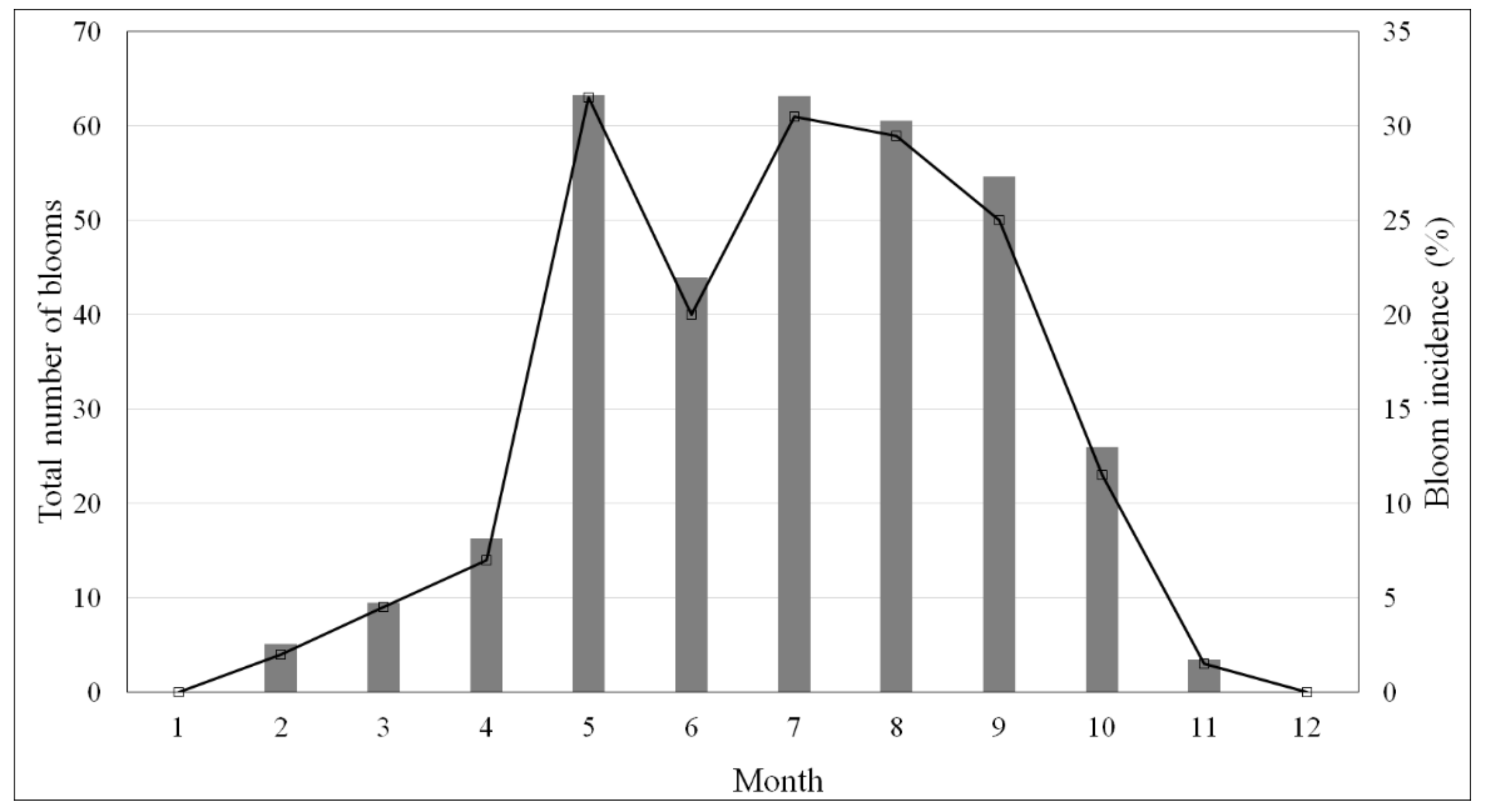
3.1.1. Pseudo-nitzschia Spp. Distribution

Pseudo-nitzschia spp. was detected (above the detection limit) in approximately 63% of samples, although only 15% were identified as bloom (abundances greater than 10⁵ cell/L). Eleven records showed abundances over 10⁶ cell/L, with a peak of 3.19 × 10⁶ cell/L and an average value of around 62,000 cells/L.

Table 4. Sampling effort (Tot.) and bloom incidence (Bloom) for each ria and year.

Year	Tot.	Bloom	Vigo		Pontevedra		Arousa		Muros
			Tot.	Bloom	Tot.	Bloom	Tot.	Bloom	Tot.	Bloom
2002	51	17	51	9	51	10	51	12	45	10
2003	52	16	52	13	52	9	52	10	49	8
2004	51	13	51	7	51	7	51	4	48	7
2005	50	18	49	11	50	14	50	10	44	12
2006	51	7	51	3	51	4	51	4	44	1
2007	51	13	51	11	51	9	51	7	44	4
2008	51	11	51	6	50	6	50	7	43	6
2009	51	18	51	12	50	11	50	10	45	6
2010	48	11	48	5	48	1	48	6	41	7
2011	51	16	51	11	50	9	48	5	42	6
2012	52	9	52	6	52	4	51	1	41	5
Total	559	149	558	94	556	84	553	76	486	72

shows the sampling effort, i.e., the total number of weeks sampled, and the bloom incidence, defined as the percentage of weeks affected by a Pseudo-nitzschia spp. bloom, for each ria and year. Note that Muros shows a lower sampling effort because this ria is not protected by islands located at the mouth (Figure 1) and hence the station M5 is more affected by severe weather situations.

Vigo was the most affected ria with 94 blooms (near 30% of the total number of blooms), followed by Pontevedra (84), Arousa (76) and Muros (72). Bloom incidences varied from 16.85% in Vigo to 13.74% in Arousa, with values around 15% in both Pontevedra and Muros (Table 4). These results differ from the ones observed in [20] for the previous decade (1992–2000), which reported Pontevedra as the most affected ria. In fact, bloom incidence was remarkably lower in Pontevedra (from 24.28% to 15.11%) and Muros (from 21.39% to 14.81%) but showed similar values in Vigo (from 17.13% to 16.85%) and Arousa (from 13.55% to 13.74%). Further research would be required to test if there was an actual change in the Pseudo-nitzschia spp. spatial distribution pattern or these variations simply fall within the expected variability.

There were remarkable variations in the bloom distribution throughout the years covered in the dataset (Table 4). The number of weeks with at least one ria affected by a Pseudo-nitzschia spp. bloom varied from 18 in 2005 and 2009 to less than 10 in 2006 and 2012. Moreover, spatial patterns were also very variable: although Vigo was generally the most affected ria (2003, 2007, 2009, 2011 and 2012), Pontevedra, Arousa and Muros showed the highest incidence in 2005, 2002 and 2010, respectively. As compared to the dataset used in [20], it is noteworthy that none of the years showed more than 20 bloom weeks as observed in 1992 and 1993.

Figure 2 shows the monthly distribution of Pseudo-nitzschia spp. in the area for the complete period (2002–2012). Most of blooms (83.74 %) were identified between May and September, while the number was very low between October and April, and even zero in December and January. The results confirm the findings of previous studies showing that Pseudo-nitzschia spp. is common in spring and late summer as a consequence of the upwelling favorable conditions [20,58]. Bloom incidence between May and September remains in values around 30% apart from a sharp decrease in June. This pattern is different from the one observed in the 1992–2002 period [20]: it almost doubles in May and September (from ~15% to ~30%) but decreases in June (from 29.27% to 21.98%) and July (from 42.47% to 31.61%). Variations could be related to changes in upwelling patterns which would need to be further researched.

3.1.2. Input Variables

In this study, we worked with the same input variables selected in [20], which were already reported to be related to the occurrence of Pseudo-nitzschia spp. blooms in the study area. These relationships were confirmed by the exploratory analysis of the dataset.

All the numerical variables are significantly positively correlated (p < 0.01) with the Pseudo-nitzschia spp. abundance (

Table 5. Basic statistics (average ± standard deviation, minimum – maximum) of each numerical variable for the complete dataset (combination A) and for no bloom and bloom classes, as well as the Pearson correlation coefficient (r) between each variable and Pseudo-nitzschia spp. abundance (transformed as log10 (1 + [Pseudo-nitzschia spp.(cells/L)]) (**significant at p < 0.01).

Variable	Complete Dataset	No Bloom	Bloom	r
Temperature	15.02 ± 1.77	14.95 ± 1.82	15.42 ± 1.43	0.25 **
	11.09–20.81	11.09–20.81	11.74–19.62
Salinity	35.12 ± 0.92	35.06 ± 0.97	35.45 ± 0.4	0.30 **
	25.46–38.05	25.46–38.05	33.49–36.03
Upwelling	170 ± 922	105 ± 904	512 ± 940	0.18 **
	−4500–6049	−4500–3468	−2445–6049
Upwelling -1day	103 ± 1005	27 ± 1021	501 ± 811	0.17 **
	−6270–6049	−6270–3592	−2198–6049
Upwelling -2 days	55 ± 1120	−28 ± 1153	491 ± 804	0.23 **
	−6858–4336	−6858–3592	−3134–4336
Upwelling -3 days	35 ± 1101	−56 ± 1129	512 ± 780	0.26 **
	−5042–4336	−5042–4275	−3134–4336
Upwelling -4 days	84 ± 1094	−4 ± 1112	541 ± 860	0.25 **
	−7971–4275	−7971–4275	−4229–3128

). Moreover, despite the fact that there is some degree of overlapping between no bloom and bloom classes (check minimum and maximum values in Table 5), significant differences (p < 0.01) were also found for each variable between both classes using Mann–Whitney tests.

The higher average temperature of bloom samples is explained by the typical seasonal pattern of Pseudo-nitzschia spp., which is more abundant in spring–summer (Figure 2). As indicated in [20], although blooms of Pseudo-nitzschia spp. often coincide with decreases in temperatures associated with upwelling events in spring–summer, temperatures in autumn and winter are even lower.

Regarding the salinity, increases in precipitation and/or river inputs lead to episodes of low salinity, which are more frequent in autumn–winter [20]. Hence, the lower average salinity of no bloom samples could be also related to the seasonal pattern.

Upwelling events (positive upwelling indices) are usually more frequent in spring–summer while downwelling events (negative upwelling indices) are common in autumn– winter [20]. Moreover, blooms of Pseudo-nitzschia spp. are usually detected during both upwelling events and the posterior relaxation period [20]. As a consequence, all the upwelling indices showed average positive values for the bloom class versus negative or nearer zero average values of no bloom samples (Table 5). Note that the maximum correlation and difference between both classes is found using the upwelling index measured three days before the sampling date (Table 5).

The occurrence of blooms of Pseudo-nitzschia spp. in the previous weeks to the observed was included because phytoplankton blooms (including Pseudo-nitzschia spp.) seem to progress along the Galician coast according to the dominant winds and currents [20,74]. Significant differences for both bloom-1w and bloom-2w between no bloom and bloom were found using Mann–Whitney tests. Around 89% of no bloom samples were not related to blooms in previous weeks (bloom-1w = 0 and bloom-1w = 0), while 47.62% and 39.12% of bloom samples showed a bloom in the previous week (bloom-1w ≥ 1) and two weeks earlier (i.e., bloom-2w ≥ 1), respectively.

The ria code and the day of the year are related to the spatial and temporal distribution of Pseudo-nitzschia spp. abundance (see Section 3.1.1). For these variables, there is not significant differences between both classes according to the Mann–Whitney tests results because of a higher overlapping.

Comparing the dataset in [20] (1992–2002) with the one used in this work (2002–2012), the slight increase in the average temperature (from 14.75° to 15.02°) and upwelling index (from 39.68 to 170.43, indicating a higher prevalence of upwelling conditions) are remarkable. Further research would be required to check if these variations are related to the climate variability.

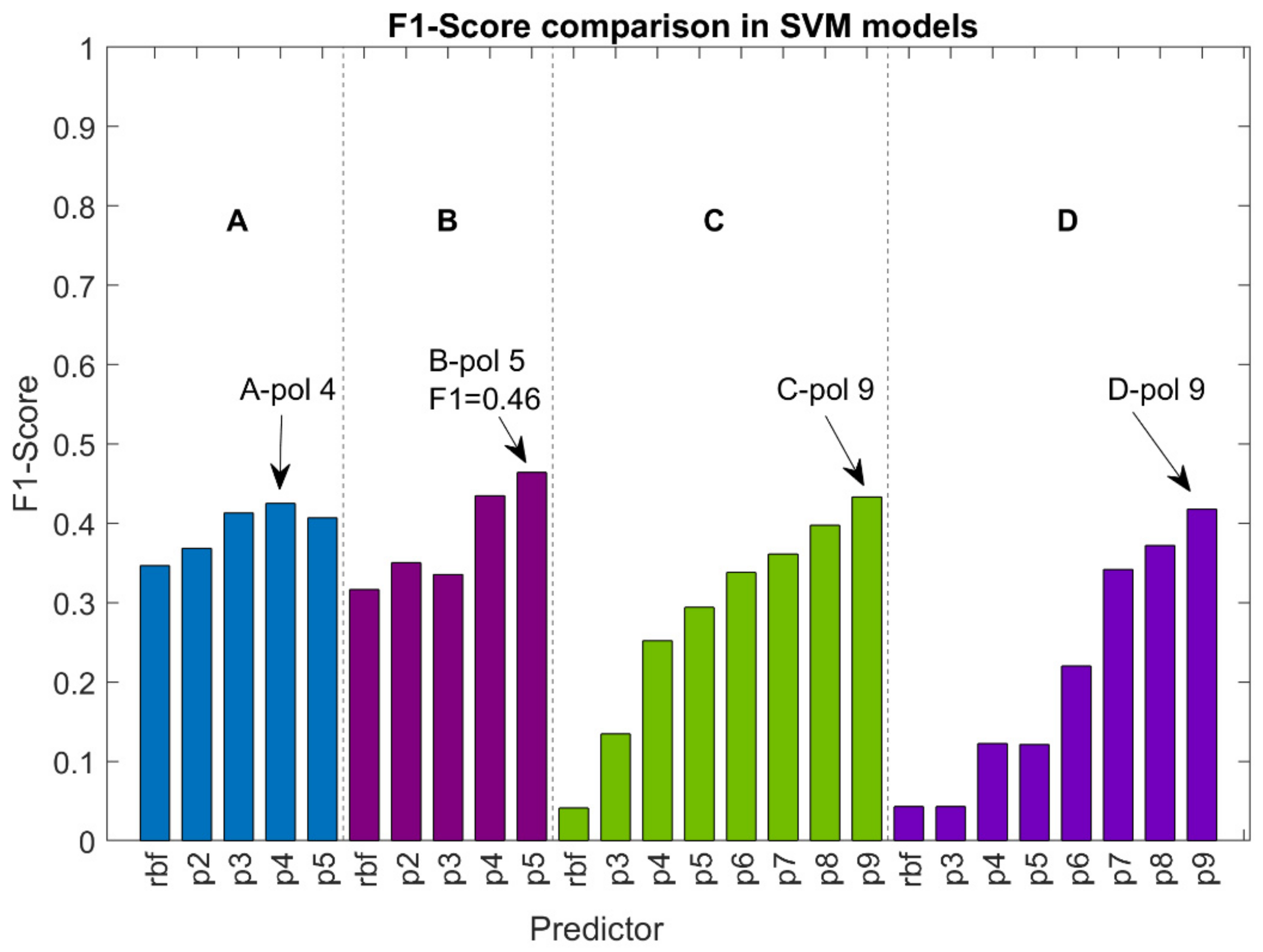
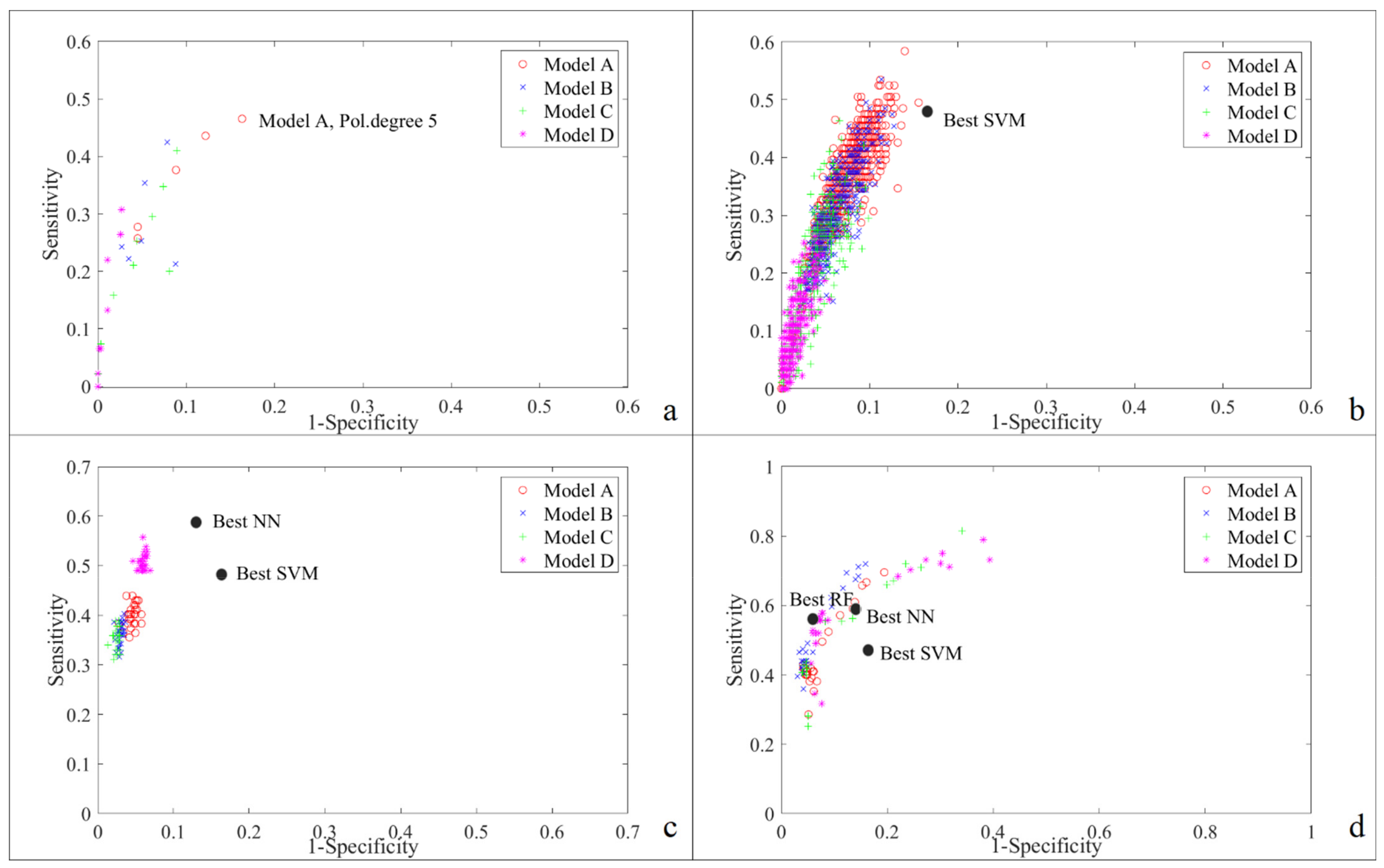
3.2. Support Vector Machines (SVM)

Figure 3 shows the F1-score computed in the validation set using SVMs with RBF and polynomial (of degrees from 2 to 9) kernels for each combination of features. Overall, polynomial kernels improve the results from the RBF kernel, with an increasing sensitivity and specificity but at the cost of an increasing number of false positives (less precision) as the polynomial degree increases.

The best global results are achieved with model B, specifically using a polynomial kernel of degree 5 (F1-score = 0.46). The best SVM with combination A is achieved with a degree of 4, while combinations C and D require a higher degree of 9.

3.3. Neural Networks (NN)

The best NN results are achieved using the combination A, although models B and C show similar results (

Table 6. Results of the multilayer perceptron (MLP) neural network (NN) with the best parametric configuration for each variable combination. Criteria for the selection of the best model are maximum F1-score (F1), minimum distance to the optimal point (0,1) in the operating receiver characteristics curve (ROC) or both (F1/ROC). All the metrics are computed from the validation set. (OA: overall accuracy; Sens.: sensitivity; Spec.: specificity; Prec.: precision; Dist. (0,1): distance to the point (0,1) in ROC curve).

Model	Criteria	OA	Sens.	Spec.	Prec.	F1-Score	Dist. (0,1)
A	F1	0.86	0.47	0.94	0.60	0.53	0.57
	ROC	0.81	0.58	0.86	0.45	0.51	0.44
B	F1/ROC	0.83	0.54	0.89	0.48	0.51	0.48
C	F1/ROC	0.86	0.46	0.93	0.56	0.51	0.54
D	F1	0.87	0.25	0.97	0.62	0.36	0.75
	ROC	0.86	0.21	0.96	0.49	0.29	0.74

). Note that model C requires more computational load (optimal achieved with 10 hidden layers) than A (six hidden layers) or B (four hidden layers). Results using combination D are poorer in terms of both F1-score and distance to point (0,1) in the ROC curve, indicating that upwelling indices are not sufficient to obtain reliable predictions using NNs.

The best global MLP NN, with a maximum F1-score of 0.53 and based on combination A, was obtained with six hidden layers, 500 iterations, and a regulation factor of 0.05. The MLP with the minimum distance to point (0,1) in the ROC, which is also based on A, shows a higher sensitivity but at the cost of a lower specificity and precision (more false positives) (Table 6).

3.4. Random Forest (RF)

Overall, RF shows good results with a good balance between sensitivity, specificity and precision, regardless of the training parameters. Unfortunately, there is also a high tendency for overfitting, with metrics near 1 in the results computed in the training set, especially in models A, B and C (

Table 7. Results of the Random Forest (RF) with the best parametric configuration for each variable combination. Criteria for the selection of the best mode are maximum F1-score (F1), minimum distance to the optimal point (0,1) in the ROC curve (ROC) or both (F1/ROC). All the metrics are computed from the validation set. (OA: Overall accuracy; Sens.: sensitivity; Spec.: specificity; Prec.: precision; Dist. (0,1): distance to the point (0,1) in ROC curve).

Model	Criteria	OA	Sens.	Spec.	Prec.	F1-Score	Dist. (0,1)
A	F1/ROC	0.87	0.44	0.96	0.71	0.54	0.56
B	F1	0.86	0.47	0.94	0.60	0.53	0.61
	ROC	0.87	0.36	0.98	0.76	0.49	0.60
C	F1/ROC	0.88	0.39	0.98	0.77	0.52	0.61
D	F1/ROC	0.88	0.59	0.94	0.64	0.60	0.45

).

However, RF tends to improve using less variables, indicating that these algorithms could be improved by including more data instead of more variables. In fact, the optimal predictor (40 bags and four variables selected as weak predictors) was based on combination D (with only five variables), with a maximum F1-score of 0.60 and a minimum distance to point (0,1) in the ROC curve of 0.45. It also shows less overfitting as compared to the other optimal models (Table 7).

3.5. AdaBoost

Unlike other machine learning methods shown in this work, AdaBoost models were selected according to the maximum F1-score and minimum distance to point (0,1) in the ROC curve being different for all the combinations of variables (

Table 8. Results of the AdaBoost models with the best parametric configuration for each variable combination. Criteria for the selection of the best model are maximum F1-score (F1), minimum distance to the optimal point (0,1) in the ROC curve (ROC) or both (F1/ROC). All the metrics are computed from the validation set. AdaBoost variant is also shown. (OA: Overall accuracy; Sens.: sensitivity; Spec.: specificity; Prec.: precision; Dist. (0,1): distance to the point (0,1) in ROC curve).

Model	Criteria	OA	Sens.	Spec.	Prec.	F1-Score	Dist. (0,1)
A	F1	0.81	0.66	0.85	0.47	0.55	0.38
	ROC	0.79	0.70	0.81	0.43	0.53	0.36
B	F1	0.84	0.69	0.88	0.55	0.61	0.33
	ROC	0.82	0.72	0.84	0.50	0.59	0.32
C	F1	0.86	0.55	0.92	0.58	0.56	0.45
	ROC	0.76	0.72	0.77	0.38	0.50	0.37
D	F1	0.87	0.57	0.93	0.61	0.59	0.44
	ROC	0.73	0.73	0.73	0.34	0.47	0.38

). In general, models with minimum distance show a higher sensitivity, but at the cost of a lower specificity and precision, producing more false positives. However, while models based on A and B present a better balance among the different metrics and similar results in both predictors, there are more marked differences between both optimal models for combinations C and D. Overall, better models were obtained using the RUSBoost variant, with the exception of the model D based on the GentleBoost maximizing F1-score.

The best global models are based on combination B, including all the variables except for the day of the year and ria. The model maximizing F1-score, trained with 200 cycles, shows a F1-score of 0.61 and a good balance between sensitivity and specificity. Results of the predictor minimizing the distance to point (0,1) in the ROC curve (based on 10 cycles) are very similar, with a slightly higher sensitivity but lower specificity. The results of the model D maximizing F1-score (F1-score = 0.59) are also remarkable, since this model uses only upwelling indices (Table 8).

4. Discussion

4.1. Models’ Performance

In general, a good binary classifier is expected to show a good balance between sensitivity and specificity, i.e., good individual accuracies for both classes (no bloom and bloom). Hence, the minimum distance to the optima point (0,1) in the ROC curve was used as one of the criteria to search for the optimal models. However, due to the unequal distribution of both classes (~15% of bloom, see Table 3), models selected according to this criterion show a high percentage of false positives (low precision). Therefore, the F1-score was also used for the selection of optimal algorithms, since this metric is considered more balanced for unbalanced datasets [91,92].

On some occasions, models with the maximum F1-score show also the minimum distance to the optimal point (0,1) in the ROC curve. Where there is a discrepancy, algorithms with the maximum F1-score generally show a lower sensitivity than the equivalent ones selected with minimum distance, but a better balance between sensitivity, specificity and precision.

Table 9. Results of the best models for each machine learning method, as well as for the SVM model based on A developed by Gonzalez Vilas at al. [20]. Subscripts indicate the criterion for model selection in the case of discrepancy between the maximizing F1-score and minimizing distance to point (0,1) in the ROC curve. All the metrics are computed from the validation set. (OA: Overall accuracy; Sens.: sensitivity; Spec.: specificity; Prec.: precision; Dist. (0,1): distance to the point (0,1) in ROC curve).

Method	Model	OA	Sens.	Spec.	Prec.	F1-Score	Dist. (0,1)
SVM (1992-2002)	A	0.79	0.77	0.79	0.41	0.53	0.32
SVM	B	0.84	0.42	0.92	0.51	0.46	0.58
NN F1	A	0.86	0.47	0.94	0.60	0.53	0.57
NNROC	A	0.81	0.58	0.86	0.45	0.51	0.44
RF	D	0.88	0.56	0.94	0.64	0.60	0.45
AdaBoostF1	BRUS 200 ci.	0.84	0.69	0.88	0.55	0.61	0.33
AdaBoostROC	BRUS 10 ci	0.82	0.72	0.84	0.50	0.59	0.32

compares the metrics computed from the validation set using the best models for each method according to both criteria, also including results from [20]. Overall, new algorithms (RF and AdaBoost) provide more suitable results than classic ones (SVM and NN), showing better values for global metrics (F1-score and distance) and a better balance between sensitivity and specificity. Classic algorithms show a higher sensitivity, but at the cost of lower specificity and precision and a high percentage of false alarms.

Figure 4 shows the ROC curves for the four methods, evincing graphically the models with a better balance between sensitivity and specificity (i.e., with a shorter distance to the optimal point (0,1)). For NNs and SVMs, better models are based on all the variables (combination A). For RF, models using variables in combination D show clearly shorter distances, evidencing that upwelling indices are sufficient to produce reliable predictions results. In case of AdaBoost, models B show the best global results. In fact, RUSBoost algorithms based on combination B show not only a short distance to the optimal point (0,1) in the ROC curve, but also high F1-score values (Table 8).

The better results obtained by new algorithms (RF and AdaBoost) could be explained by several reasons. Firstly, classic algorithms require data scaling since they rely on homogenous feature ranges to work properly. However, scaling has no impact on the performance of RF and AdaBoost [85,86,90]. Secondly, the combination of learners of ensemble methods leads to a better bias/variance tradeoff and an improvement of the generalization ability as compared to algorithms relying on single hypothesis [16,86]. Note that results were computed from a validation subset that was not used in the training procedure. Finally, results also seem to indicate a better adaptation of ensemble algorithms (RF and AdaBoost) to unbalanced datasets [93,94].

Comparing the classical algorithms, MLP improved SVMs despite the fact that SVMs are expected to be a more robust technique for two-class classification problems. However, the SVM results seem to be more affected by the imbalance between both classes. The learning curve (Figure 5) shows some overfitting, so that the model tends to better predict the most frequent class (no bloom) leading to a higher specificity but at the cost of a lower sensitivity. Weighted SVM, i.e., the application of a different weight for each class to correct the imbalance effect [20], could improve the results. On the other hand, the learning curve for MLP (Figure 5) indicates an underfitting situation, and hence the model would be expected to improve by adding new variables.

Between RF and AdaBoost, AdaBoost works slightly better. Although the best RF model shows the best values of overall accuracy, specificity and precision, it fails in sensitivity as compared to AdaBoost models, which show the highest sensitivities for the decade 2001–2012 and the best balance between metrics, leading to the maximum F1-score and the minimum distance to the point (0,1) in ROC curve.

As with the SVM, the learning curve of the best RF algorithm (model D, Figure 5) evidences some overfitting, leading to a higher accuracy of the majority class (no bloom) and a lower sensitivity as compared to AdaBoost. In general, models with overfitting are expected to be improved by increasing the number of samples. In case of RF, variance error can be also lowered by reducing the model complexity (i.e., the number of individual decision trees) selecting less input variables. In fact, as explained in Section 3.3, overfitting is clear with RF based on A, B and C, with an almost perfect fitting observed in the training set, while model D shows better results. Note that this model, despite of working with less variables, uses more input samples due to the availability of more valid records (see Table 2 and Table 3).

In the case of AdaBoost, the learning curve (Figure 5) of the best model indicates some underfitting, and hence the model could be improved with another selection of input variables. The number of samples does not seem to be critical, since the training error remains more or less constant over 1000 training samples.

One of the main limitations of modelling blooms of Pseudo-nitzschia spp. in Galicia is the imbalance in the dataset. Results could be improved by building a balanced dataset through the selection of a number of no bloom samples approximately equal to the number of bloom records. However, this process could lead to a loss of important information for the discrimination of both classes.

Future work could include the development of specific models for a ria and/or time period to work with more balanced datasets. For instance, for the period from May to September, which sums up more than 80% of all the Pseudo-nitzschia spp. events (see Section 3.1.1), the dataset would include near 30% of bloom (70% of no bloom) samples. However, in addition to their limited temporal and/or spatial applicability, the smaller number of records or the loss of key information might affect the results.

In this study, we trained the models using 2/3 of the total records, using the remaining records (1/3) as an independent set for validation. The comparison of models developed using a growing number of training samples (e.g., 2/3, 3/4 and 4/5), and hence less records for the validation (e.g., 1/3, 1/4 and 1/5), would be an interesting approach for gaining insight into the generalization capability of the different machine learning techniques or feature combinations.

This work mainly focused on the comparison of different machine learning techniques, so that models were developed using default options and a simple grid-search approach for selecting the optimal values of their main parameters. Therefore, all the results could be improved by a finer adjustment or the application of advanced approaches in the pre-processing steps, as scaling (for SVM and MLP) or feature selection.

4.2. Variable Contribution

Despite the correlations found between the input variables and the Pseudo-nitzschia spp. abundance (Table 5), discrimination between bloom and no bloom classes is a complex and non-linear problem. None of the variables themselves are sufficient to identify bloom conditions because of the overlapping between both classes.

Overall, models B perform better than models C and similar or better than models A (e.g., AdaBoost, see Table 8), indicating the importance of the occurrence of blooms in the previous week for the predictions. In contrast, several models work correctly without temporal (day of the year) or spatial (ria) information. Note that significant differences between both classes were not found for these two variables using Mann–Whitney tests (see Section 3.1.2), while other variables are directly related to the temporal (e.g., temperature, salinity, upwelling indices) and spatial (bloom occurrence in previous weeks) distribution patterns of Pseudo-nitzschia spp.

Upwelling indices seem to be a critical and necessary variable for prediction, since even models running only with upwelling indices (model D) achieve reasonable results (e.g., RF, see Table 7). Upwelling indices include several positive and negative peaks, so that the good results achieved by RF/D could be explained by its robustness to outliers as compared to other algorithms [41].

The inclusion of new variables could improve the results, especially for models showing underfitting in the learning curves (MLP and AdaBoost). Without using new datasets, variations of temperature or salinity from the previous to the present week could provide important information about the evolution of Pseudo-nitzschia spp. blooms.

Chlophyll-a concentration is a good proxy for phytoplankton abundance. Spyrakos et al. [74] showed the potential of satellite regional chlorophyll-a algorithms to detect “patches” of high Pseudo-nitzschia abundances in the rias. Several authors have proposed the use of satellite data (chlorophyll-a concentration, sea surface temperature) as an input of Pseudo-nitzschia spp. prediction models [61,63,65].

The relationship between the abundance of Pseudo-nitzschia spp. and the concentrations of different nutrients (mainly nitrate, nitrite, phosphate and silicate) have been extensively analyzed in observational studies [95,96]. Defining the role of nutrients is a challenging task since concentrations vary during the bloom development and hence relationships can be different depending of the instant in which the abundance is measured. Even so, nutrients concentrations have been successfully included as a forcing driver in Pseudo-nitzschia spp. prediction models [6,8,41].

Other interesting variables could be river input or precipitation, as indirect indicators of the input of nutrients though freshwater discharges. Note that this effect is included, to some extent, in the salinity values. Moreover, some authors ([97] and references therein) have indicated that upwelling is the main source of nutrients in the Rias Baixas area, while freshwater discharges play a less important role.

4.3. Comparison with Other Works

SVM algorithms with data from 1992 to 2002 [20], show a good sensitivity, but at the cost of a high number of false positives, showing a poorer specificity and precision as compared to RF or AdaBoost (Table 9). However, it improves the best SVM for the decade 2002–2012 considering both F1-score and distance to the point (0,1) in the ROC curve. This better performance could be explained because SVMs developed by [20] include a finer adjustment of the models, using a different weight for each class to correct the imbalance effect.

The best-fit linear model for Pseudo-nitzschia spp. abundance developed by [61] for the Santa Barbara Channel was able to correctly classify around 75% of bloom observations and 93% of no bloom observations, resulting in an excellent F1-score of 0.82. Results are not directly comparable, since they worked with a small (n = 77) and balanced dataset with a log-normal distribution of the Pseudo-nitzschia spp. abundance, used a different threshold to discriminate between no bloom and bloom classes and input features included data from satellite images and nutrient concentrations.

Good results were also found by [8] using logistic regression for the annual and seasonal prediction of toxigenic blooms of Pseudo-nitzschia spp. in the Monterey Bay (California), using temperature, salinity, upwelling indices, nutrient concentrations and river flow as input features. Working with more balanced datasets (around 40% of blooms, between 207 and 222 samples), they reported F1-score values between 0.70 and 0.76 in their best models.

Using similar input features as [8] and a long-term 22-year dataset, a logistic generalized linear model (GLM) approach was developed to predict potentially toxigenic Pseudo-nitzschia blooms in the Chesapeake Bay [6], reporting optimal values of sensitivity and precision of 0.75 and 0.48, respectively. They worked with unbalanced datasets (around 10% of blooms with a 100 cell/L threshold), but applied lower thresholds (10, 100 and 1000 cell/L) than in our work to discriminate no bloom and bloom classes.

5. Conclusions

In this work, we have developed a set of models to predict the appearance of Pseudo-nitzschia spp. blooms in the Rias Baixas area on a specific date and ria. The models are based on variables that can be operationally monitored and/or predicted in the short-term, and hence could be easily implemented to establish an early warning system. This system could provide useful information to the local mussel producers to complement the monitoring program and help to mitigate the potential impact of blooms on mussel production and public health.

Blooms are defined in terms of overall abundance (10⁵ cells/L). Therefore, an important limitation is that toxic blooms are not discriminated, considering that DA production depends on the species and not all the blooms are toxic [14]. Although data on specific species are not available, there is limited information about the closure of mussel floating farming parks caused by ASP and DA concentration on molluscs (only since 2016), which could be useful for discrimination toxic blooms and improve the models in future. New variables, e.g., nutrient concentrations or vertical distributions, could also be introduced to improve the algorithms.

Models maximizing the F1-score were selected as the optimal ones to establish a HAB prediction system because they are expected to show a high sensitivity (if a bloom occurs in the study area, the system must predict it) and precision (if a bloom is predicted, it must exist) [60]. However, if users are more interested in predicting more blooms at the cost of more false alarms, models minimizing the distance to the optimal point (0,1) in ROC curve could be a better option.

HAB prediction systems will be more accurate if they include monitoring data with a higher temporal frequency and spatial coverage. For instance, the analysis of map products derived from optical satellite images, including chlorophyll-a concentration or species indicators, could complement the existing monitoring program based on direct observations [98]. Moreover, the development of automated sensor systems with a high frequency of measurements at different stations and depths, or the use of drones will allow a breakthrough in the detection of toxic algae development events in coastal systems.

Finally, machine learning methods could also be useful for studying potential changes in the distribution patters of HAB-forming species associated with climate variability.

References

1. Gobler, C.J.; Doherty, O.M.; Hattenrath-Lehmann, T.K.; Griffith, A.W.; Kang, Y.; Litaker, R.W. Ocean warming since 1982 has expanded the niche of toxic algal blooms in the North Atlantic and North Pacific oceans. Proc. Natl. Acad. Sci. USA 2017, 114, 4975–4980. [Google Scholar] [CrossRef] [PubMed] [Green Version]
2. Griffith, A.W.; Gobler, C.J. Harmful algal blooms: A climate change co-stressor in marine and freshwater ecosystems. Harmful Algae 2020, 91, 101590. [Google Scholar] [CrossRef] [PubMed]
3. Anderson, D.; Cembella, A.; Hallegraeff, G. Progress in understanding harmful algal blooms: Paradigm shifts and new technologies for research, monitoring, and management. Ann. Rev. Mar. Sci. 2012, 4, 143–176. [Google Scholar] [CrossRef] [Green Version]
4. Anderson, D.M. Approaches to monitoring, control and management of harmful algal blooms (HABs). Ocean Coast Manag. 2009, 52, 342. [Google Scholar] [CrossRef] [Green Version]
5. Anderson, C.R.; Moore, S.K.; Tomlinson, M.C.; Silke, J.; Cusack, C.K. Living with harmful algal blooms in a changing world: Strategies for modeling and mitigating their effects in coastal marine ecosystems. In Coastal and Marine Hazards, Risks, and Disasters; Shroeder, J.F., Ellis, J.T., Sherman, D.J., Eds.; Elsevier: Amsterdam, The Netherlands, 2015; pp. 495–561. [Google Scholar]
6. Anderson, C.R.; Mathew Sapiano, R.P.; Krishna Prasad, M.B.; Long, W.; Tango, P.J.; Brown, C.W.; Murtugudde, R. Predicting potentially toxigenic Pseudo-nitzschia blooms in the Chesapeake Bay. J. Mar. Syst. 2010, 83, 127–140. [Google Scholar] [CrossRef]
7. Manning, N.F.; Wang, Y.-C.; Long, C.M.; Bertani, I.M.; Sayers, J.; Bosse, K.R.; Shuchman, R.A.; Scavia, D. Extending the forecast model: Predicting Western Lake Erie harmful algal blooms at multiple spatial scales. J. Great Lakes Res. 2019, 45, 587–595. [Google Scholar] [CrossRef]
8. Lane, J.; Raimondi, P.T.; Kudela, R.M. Development of a logistic regression model for the prediction of toxigenic Pseudo-nitzschia blooms in Monterey Bay, California. Mar. Ecol. Prog. Ser. 2009, 383, 37–51. [Google Scholar] [CrossRef] [Green Version]
9. Raine, R.; McDermott, G.; Silke, J.; Lyons, K.; Nolan, G.; Cusack, C. A simple short range model for the prediction of harmful algal events in the bays of southwestern Ireland. J. Mar. Syst. 2010, 83, 150–157. [Google Scholar] [CrossRef]
10. Volf, G.; Atanasova, N.; Kompare, B.; Precali, R.; Ožanić, N. Descriptive and prediction models of phytoplankton in the northern Adriatic. Ecol. Model. 2011, 222, 2502–2511. [Google Scholar] [CrossRef]
11. McGowan, J.A.; Deyle, E.R.; Ye, H.; Carter, M.L.; Perretti, C.T.; Seger, K.D.; de Verneil, A.; Sugihara, G. Predicting coastal algal blooms in southern California. Ecology 2017, 98, 1419–1433. [Google Scholar] [CrossRef] [Green Version]
12. Derot, J.; Yajima, H.; Jacquet, S. Advances in forecasting harmful algal blooms using machine learning models: A case study with Planktothrix rubescens in Lake Geneva. Harmful Algae 2020, 99, 101906. [Google Scholar] [CrossRef]
13. Huettmann, F.; Craig, E.H.; Herrick, K.A.; Baltensperger, A.P.; Humphries, G.R.W.; Lieske, D.J.; Miller, K.; Mullet, T.C.; Oppel, S.; Resendiz, C.; et al. Use of machine learning (ML) for predicting and analyzing ecological and ‘presence only’ data: An overview of applications and a good outlook. In Machine Learning for Ecology and Sustainable Natural Resource Management; Humphries, G., Magness, D.R., Huettmann, F., Eds.; Springer International Publishing: Cham, Switzerland, 2018; pp. 27–61. [Google Scholar]
14. Ralston, R.; Moore, S.K. Modeling harmful algal blooms in a changing climate. Harmful Algae 2020, 91, 101729. [Google Scholar] [CrossRef]
15. Rousso, B.Z.; Bertone, E.; Stewart, R.; Hamilton, D.P. A systematic literature review of forecasting and predictive models for cyanobacteria blooms in freshwater lakes. Water Res. 2020, 182, 115959. [Google Scholar] [CrossRef]
16. Yu, P.; Gao, R.; Zhang, D.; Liu, Z.-P. Predicting coastal algal blooms with environmental factors by machine learning methods. Ecol. Indic. 2021, 123, 107334. [Google Scholar] [CrossRef]
17. Boser, B.E.; Guyon, I.M.; Vapnik, V.N. A training algorithm for optimal margin classifiers. In Proceedings of the Fifth Annual Workshop on Computational Learning Theory, Pittsburgh, PA, USA, 27–29 July 1992; Association for Computing Machinery: New York, NY, USA, 1992. [Google Scholar]
18. Vapnik, V. The Support Vector method of function estimation. In Nonlinear Modeling; Suykens, J.A.K., Vandewalle, J., Eds.; Springer: Boston, MA, USA, 1998; pp. 55–85. [Google Scholar]
19. Vapnik, V.N. The Nature of Statistical Learning Theory; Springer: New York, NY, USA, 2000. [Google Scholar]
20. González Vilas, L.; Spyrakos, E.; Torres Palenzuela, J.M.; Pazos, Y. Support Vector Machine-based method for predicting Pseudo-nitzschia spp. blooms in coastal waters (Galician rias, NW Spain). Prog. Oceanogr. 2014, 124, 66–77. [Google Scholar] [CrossRef]
21. Chen, S.; Xie, Z.; Lou, I.; Ung, W.K.; Mok, K.M. Freshwater Algal Bloom Prediction by Support Vector Machine in Macau Storage Reservoirs. Math. Probl. Eng. 2012, 2012, 397473. [Google Scholar]
22. García Nieto, P.J.; Alonso Fernández, J.R.; González Suárez, V.M.; Díaz Muñiz, C.; García-Gonzalo, E.; Mayo Bayón, R. A hybrid PSO optimized SVM-based method for predicting of the cyanotoxin content from experimental cyanobacteria concentrations in the Trasona reservoir: A case study in Northern Spain. Appl. Math. Comput. 2015, 260, 170–187. [Google Scholar]
23. Ribeiro, R.; Torgo, L. A comparative study on predicting algae blooms in Douro River, Portugal. Ecol. Model. 2008, 212, 86–91. [Google Scholar] [CrossRef] [Green Version]
24. Lou, I.; Xie, Z.; Ung, W.K.; Mok, K.M. Integrating support vector regression with particle swarm optimization for numerical modeling for algal blooms of freshwater. Appl. Math. Model. 2015, 39, 5907–5916. [Google Scholar] [CrossRef]
25. Shen, J.; Qin, Q.; Wang, Y.; Sisson, M. A data-driven modeling approach for simulating algal blooms in the tidal freshwater of James River in response to riverine nutrient loading. Ecol. Model. 2019, 398, 44–54. [Google Scholar] [CrossRef] [Green Version]
26. Bourel, M.; Crisci, C.; Martínez, A. Consensus methods based on machine learning techniques for marine phytoplankton presence–absence prediction. Ecol. Inf. 2017, 42, 46–54. [Google Scholar] [CrossRef]
27. Gokaraju, B.; Durbha, S.S.; King, R.L.; Younan, N.H. A machine learning based spatio-temporal data mining approach for detection of harmful algal blooms in the Gulf of Mexico. IEEE J. Sel. Top. Appl. Earth Obs. Remote Sens. 2011, 4, 710–720. [Google Scholar] [CrossRef]
28. Hill, P.R.; Kumar, A.; Temimi, M.; Bull, D.R. HABNet: Machine Learning, Remote Sensing-Based Detection of Harmful Algal Blooms. IEEE J. Sel. Top. Appl. Earth Obs. Remote Sens. 2020, 13, 3229–3239. [Google Scholar] [CrossRef]
29. Li, X.; Yu, J.; Jia, Z.; Song, J. Harmful algal blooms prediction with machine learning models in Tolo Harbour. In Proceedings of the International Conference on Smart Computing, Hong Kong, China, 3–5 November 2014; IEEE Computer Society: Washington, DC, USA, 2015; pp. 245–250. [Google Scholar]
30. Lek, S.; Delacoste, M.; Baran, P.; Lauga, J.; Aulagnier, S. Application of neural network for nonlinear modeling in ecology. Ecol. Model. 1996, 90, 39–52. [Google Scholar] [CrossRef]
31. McCulloch, W.S.; Pitts, W. A Logical Calculus of the Ideas Immanent in Nervous Activity. Bull. Math. Biol. 1990, 52, 99–115. [Google Scholar] [CrossRef]
32. Recknagel, F.; Bobbin, J.; Whigham, P.; Wilson, H. Comparative application of artificial neural networks and genetic algorithms for multivariate time-series modelling of algal blooms in freshwater lakes. J. Hydroinform. 2002, 4, 125–133. [Google Scholar] [CrossRef] [Green Version]
33. Wei, B.; Sugiura, N.; Maekawa, T. Use of artificial neural network in the prediction of algal blooms. Water Res. 2001, 35, 2022–2028. [Google Scholar] [CrossRef]
34. Xiao, X.; He, J.; Huang, H.; Miller, T.R.; Christakos, G.; Reichwaldt, E.S.; Ghadouani, A.; Lin, S.; Xu, X.; Shi, J. A novel single-parameter approach for forecasting algal blooms. Water Res. 2017, 108, 222–231. [Google Scholar] [CrossRef]
35. Brown, C.W.; Hood, R.R.; Long, W.; Jacobs, J.; Ramers, D.; Wazniak, C.; Wiggert, J.; Wood, R.; Xu, J. Ecological forecasting in Chesapeake Bay: Using a mechanistic–empirical modeling approach. J. Mar. Syst. 2013, 125, 113–125. [Google Scholar] [CrossRef]
36. Guallar, C.; Delgado, M.; Diogène, J.; Fernández-Tejedor, M. Artificial neural network approach to population dynamics of harmful algal blooms in Alfacs Bay (NW Mediterranean): Case studies of Karlodinium and Pseudo-nitzschia. Ecol. Model. 2016, 338, 37–50. [Google Scholar] [CrossRef]
37. Lee, J.H.W.; Huang, Y.; Dickman, M.; Jayawardena, A.W. Neural network modelling of coastal algal blooms. Ecol. Model. 2003, 159, 179–201. [Google Scholar] [CrossRef]
38. Velo-Suarez, L.; Gutierrez-Estrada, J.C. Artificial neural network approaches to one-step weekly prediction of Dinophysis acuminata blooms in Huelva (Western Andalucia, Spain). Harmful Algae 2007, 6, 361–371. [Google Scholar] [CrossRef]
39. Coad, P.; Cathers, B.; Ball, J.E.; Kadluczka, R. Proactive management of estuarine algal blooms using an automated monitoring buoy coupled with an artificial neural network. Environ. Model. Softw. 2014, 61, 393–409. [Google Scholar] [CrossRef]
40. Tian, W.; Liao, Z.; Zhang, J. An optimization of artificial neural network model for predicting chlorophyll dynamics. Ecol. Model. 2017, 364, 42–52. [Google Scholar] [CrossRef]
41. Breiman, L. Random Forests. Mach. Learn. 2001, 45, 5–32. [Google Scholar] [CrossRef] [Green Version]
42. Liu, Y.; Wu, H. Water bloom warning model based on random forest. In Proceedings of the 2017 International Conference on Intelligent Informatics and Biomedical Sciences (ICIIBMS), Okinawa, Japan, 24–26 November 2017; Institute of Electrical and Electronics Engineers (IEEE): New York, NY, USA, 2018; pp. 45–48. [Google Scholar]
43. Evans, J.S.; Murphy, M.A.; Holden, Z.A.; Cushman, S.A. Modeling Species Distribution and Change Using Random Forest. In Predictive Species and Habitat Modeling in Landscape Ecology; Drew, C., Wiersma, Y., Huettmann, F., Eds.; Springer: New York, NY, USA, 2011; pp. 139–159. [Google Scholar]
44. Wei, C.L.; Rowe, G.T.; Escobar-Briones, E.; Boetius, A.; Soltwedel, T.; Caley, M.J.; Soliman, Y.; Huettmann, F.; Qu, F.; Yu, Z.; et al. Global Patterns and Predictions of Seafloor Biomass Using Random Forests. PLoS ONE 2010, 5, 15323. [Google Scholar] [CrossRef] [PubMed]
45. Derot, J.; Yajima, H.; Schmitt, J. Benefits of machine learning and sampling frequency on phytoplankton bloom forecasts in coastal areas. Ecol. Inf. 2020, 60, 101174. [Google Scholar] [CrossRef]
46. Harley, J.R.; Lanphier, K.; Kennedy, E.; Whitehead, C.; Bidlack, J.R. Random forest classification to determine environmental drivers and forecast paralytic shellfish toxins in Southeast Alaska with high temporal resolution. Harmful Algae 2020, 99, 101918. [Google Scholar] [CrossRef]
47. Valbi, E.; Ricci, F.; Capellacci, S.; Casabianca, S.; Scardi, M.; Penna, A. A model predicting the PSP toxic dinoflagellate Alexandrium minutum occurrence in the coastal waters of the NW Adriatic Sea. Sci. Rep. 2019, 9, 4166. [Google Scholar] [CrossRef] [Green Version]
48. Yñiguez, A.T.; Ottong, Z.J. Predicting fish kills and toxic blooms in an intensive mariculture site in the Philippines using a machine learning model. Sci. Total Environ. 2020, 707, 136173. [Google Scholar] [CrossRef]
49. Freund, Y.; Schapire, R.E. A Decision-Theoretic Generalization of On-Line Learning and an Application to Boosting. J. Comput. Syst. Sci. 1997, 55, 119–139. [Google Scholar] [CrossRef] [Green Version]
50. Kadavi, P.R.; Lee, C.-W.; Lee, S. Application of Ensemble-Based Machine Learning Models to Landslide Susceptibility Mapping. Remote Sens. 2018, 10, 1252. [Google Scholar] [CrossRef] [Green Version]
51. Peng, L.; Liu, K.; Cao, J.; Zhu, Y.; Li, F.; Liu, L. Combining GF-2 and RapidEye satellite data for mapping mangrove species using ensemble machine-learning methods. Int. J. Remote Sens. 2020, 41, 813–838. [Google Scholar] [CrossRef]
52. Tran, T.; Hoang, N. Predicting algal appearance on mortar surface with ensembles of adaptive neuro fuzzy models: A comparative study of ensemble strategies. Int. J. Mach. Learn. Cyber. 2019, 10, 1687–1704. [Google Scholar] [CrossRef]
53. Stumpf, R.P.; Tomlinson, M.C.; Calkins, J.A.; Kirkpatrick, B.; Fisher, K.; Nierenberg, K.; Currier, R.; Wynne, T.T. Skill assessment for an operational algal bloom forecast system. J. Mar. Syst. 2009, 76, 151–161. [Google Scholar] [CrossRef] [PubMed] [Green Version]
54. Hallegraeff, G.M. Harmful Algal Blooms: A global overview. In Manual on Harmful Marine Microalgae; Hallegraeff, G.M., Anderson, D.M., Cembella, E.D., Eds.; UNESCO: Paris, France, 2004; Volume 33, pp. 25–80. [Google Scholar]
55. Bates, S.S.; Garrison, D.L.; Horner, R.A. Bloom dynamics and physiology of domoic-acid-producing Pseudo-nitzschia species. In The Physiological Ecology of Harmful Algal Blooms; Anderson, D.M., Cembella, E.D., Hallegraeff, G.M., Eds.; Springer: Berlin/Heidelberg, Germany, 1998; pp. 267–292. [Google Scholar]
56. Anderson, C.R.; Brzezinski, M.A.; Washburn, L.; Kudela, R. Circulation and environmental conditions during a toxigenic Pseudo-nitzschia australis bloom in the Santa Barbara Channel, California. Mar. Ecol. Prog. Ser. 2006, 327, 119–133. [Google Scholar] [CrossRef]
57. Fraga, S.; Alvarez, M.J.; Míguez, A.; Fernández, M.L.; Costas, E.; Lopez-Rodas, V. Pseudo-nitzschia species isolated from Galician waters: Toxicity, DNA content and lectin binding assay. In Harmful Algae; Reguera, B., Blanco, B., Fernández, M.L., Wyatt, T., Eds.; Xunta de Galicia and Intergovernmental Commission of UNESCO: Santiago de Compostela, Spain, 1998; pp. 270–273. [Google Scholar]
58. Palma, S.; Mouriño, H.; Silva, A.; Barao, M.; Moita, M.T. Can Pseudo-nitzschia blooms be modeled by coastal upwelling in Lisbon Bay? Harmful Algae 2010, 9, 294–303. [Google Scholar] [CrossRef]
59. Louw, D.C.; Doucette, G.J.; Lundholm, N. Morphology and toxicity of Pseudo-nitzschia species in the northern Benguela Upwelling System. Harmful Algae 2018, 75, 118–128. [Google Scholar] [CrossRef] [PubMed]
60. Blum, I.; Rao, D.S.; YouLian, P.; Swaminathan, S.; Adams, N.G.; Subba Rao, D.V. Development of statistical models for prediction of the neurotoxin domoic acid levels in the pennate diatom Pseudo-nitzschia pungens f. multiseries utilizing data from cultures and natural blooms. In Algal Cultures, Analogues of Blooms and Applications; Subba Rao, D.V., Ed.; Science Publishers: Enfield, CT, USA, 2006; Volume 2, pp. 891–916. [Google Scholar]
61. Anderson, C.R.; Seigel, D.A.; Kudela, R.; Brzezinski, M.A. Empirical models of toxigenic Pseudo-nitzschia blooms: Potential use as a remote detection tool in the Santa Barbara Channel. Harmful Algae 2009, 8, 478–492. [Google Scholar] [CrossRef]
62. Terseleer, N.; Gypens, N.; Lancelot, C. Factors controlling the production of domoic acid by Pseudo-nitzschia (Bacillariophyceae): A model study. Harmful Algae 2013, 24, 45–53. [Google Scholar] [CrossRef]
63. Sacau-Cuadrado, M.; Conde-Pardo, P.; Otero-Tranchero, P. Forecast of red tides off the Galician coast. Acta Astronaut. 2003, 53, 439–443. [Google Scholar] [CrossRef]
64. Cusack, C.; Mouriño, H.; Moita, M.T.; Silke, J. Modelling Pseudo-nitzschia events off southwest Ireland. J. Sea Res. 2015, 105, 30–41. [Google Scholar] [CrossRef]
65. Cusack, C.; Dabrowski, T.; Lyons, K.; Berry, A.; Westbrook, G.; Salas, R.; Duffy, C.; Nolan, G.; Silke, J. Harmful algal bloom forecast system for SW Ireland. Part II: Are operational oceanographic models useful in a HAB warning system. Harmful Algae 2016, 53, 86–101. [Google Scholar] [CrossRef]
66. Giddings, S.N.; MacCready, P.; Hickey, B.M.; Banas, N.S.; Davis, K.A.; Siedlecki, S.A.; Trainer, V.L.; Kudela, R.M.; Pelland, N.A.; Connolly, T.P. Hindcasts of potential harmful algal bloom transport pathways on the Pacific Northwest coast. J. Geophys. Res. Ocean. 2014, 119, 2439–2461. [Google Scholar] [CrossRef]
67. Townhill, B.L.; Tinker, J.; Jones, M.; Pitois, S.; Creach, V.; Simpson, S.D.; Dye, S.; Bear, E.; Pinnegar, J.K. Harmful algal blooms and climate change: Exploring future distribution changes. Ices J. Mar. Sci. 2018, 75, 1882–1893. [Google Scholar] [CrossRef] [Green Version]
68. Wooster, W.S.; Bakun, A.; McLain, D.R. The seasonal upwelling cycle along the Eastern boundary of the North Atlantic. J. Mar. Res. 1976, 34, 131–141. [Google Scholar]
69. Fraga, F. Upwelling off the Galician coast, northwest Spain. In Coastal Upwelling; Richardson, F.A., Ed.; American Geophysical Union: Washington, DC, USA, 1981; pp. 176–182. [Google Scholar]
70. Blanton, J.O.; Tenore, K.R.; Castillejo, F.F.; Atkinson, L.P.; Schwing, F.B.; Lavín, A. The relationship of upwelling to mussel production in the rías of western coast of Spain. J. Mar. Res. 1987, 45, 497–511. [Google Scholar] [CrossRef] [Green Version]
71. Bode, A.; Varela, M.; Barquero, S.; Ossorio-Alvarez, M.; Gonzalez, N. Preliminary Studies on the Export of Organic Matter During Phytoplankton Blooms off La Coruña (Northwestern Spain). J. Mar. Biol. Assoc. UK 1998, 78, 1–15. [Google Scholar] [CrossRef]
72. Labarta, U.; Fernández-Reiriz, M.J. The Galician mussel industry: Innovation and changes in the last forty years. Ocean Coast. Manag. 2019, 167, 208–218. [Google Scholar] [CrossRef]
73. Avdelas, L.; Avdic-Mravlje, E.; Borges Marques, A.C.; Cano, S.; Capelle, J.J.; Carvalho, N.; Cozzolino, M.; Dennis, J.; Ellis, T.; Fernández Polanco, J.M.; et al. The decline of mussel aquaculture in the European Union: Causes, economic impacts and opportunities. Rev. Aquacult. 2021, 13, 91–118. [Google Scholar] [CrossRef]
74. Spyrakos, E.; González Vilas, L.; Torres Palenzuela, J.M.; Barton, E.D. Remote sensing chlorophyll a of optically complex waters (rias Baixas, NW Spain): Application of a regionally specific chlorophyll an algorithm for MERIS full resolution data during an upwelling cycle. Remote Sens. Environ. 2011, 115, 2471–2485. [Google Scholar] [CrossRef] [Green Version]
75. Margalef, R. Estructura y dinámica de la “purga de mar” en Ría de Vigo. Investig. Pesq. 1956, 5, 113–134. [Google Scholar]
76. Tilstone, G.H.; Figueiras, F.G.; Fraga, F. Upwelling-Downwelling Sequences in the Generation of Red Tides in a Coastal Upwelling System. Mar Ecol. Progr. Ser. 1994, 112, 241–253. [Google Scholar] [CrossRef]
77. Figueiras, F.G.; Jones, K.J.; Mosquera, A.M.; Alvarez-Salgado, X.A.; Edwards, A.; Macdougall, N. Red Tide Assemblage Formation in an Estuarine Upwelling Ecosystem—Ria-De-Vigo. J. Plankton Res. 1994, 16, 857–878. [Google Scholar] [CrossRef]
78. GEOHAB. Global Ecology and Oceanography of Harmful Algal Blooms. In GEOHAB Core Research Project: HABs in Upwelling Systems; Pitcher, P., Moita, T., Trainer, V.L., Kudela, R., Figueiras, P., Probyn, T., Eds.; IOC: Paris, France; SCOR: Baltimore, MD, USA, 2005; pp. 11–82. [Google Scholar]
79. Figueiras, F.G.; Pazos, Y. Hydrography and phytoplankton of the Ría de Vigo before and during a red tide of Gymnodinium catenatum Graham. J. Plankton Res. 1991, 13, 589–608. [Google Scholar] [CrossRef]
80. Alvarez-Salgado, X.A.; Labarta, U.; Fernández-Reiriz, M.J.; Figueiras, F.G.; Roson, G.; Piedracoba, S.; Filgueira, R.; Cabanas, J.M. Renewal time and the impact of harmful algal blooms on the extensive mussel raft culture of the Iberian coastal upwelling system (SW Europe). Harmful Algae 2008, 7, 849–855. [Google Scholar] [CrossRef] [Green Version]
81. Rodríguez, G.R.; Villasante, S.; García-Negro, M.C. Are red tides affecting economically the commercialization of the Galician (NW Spain) mussel farming? Mar. Policy 2011, 35, 252–257. [Google Scholar] [CrossRef]
82. Utermöhl, H. Zur vervollkommnung der quantitativen phytoplankton-methodik. Mitt. Int. Ver. Theor. Unde Amgewandte Limnol. 1958, 9, 1–38. [Google Scholar] [CrossRef]
83. Herrera, J.L.; Piedracoba, S.; Varela, R.A.; Roson, G. Statial analysis of the wind field on the western coast of Galicia (NW Spain) from in situ measurements. Cont. Shelf Res. 2005, 25, 1728–1748. [Google Scholar] [CrossRef]
84. Bakun, A. Coastal Upwelling Indexes, West Coast of North America, 1946–1971; NOAA Technical Report NMFS SSRF-671; U.S. Department of Commerce: Seattle, WA, USA, 1973; pp. 1–103.
85. Sarle, W.S. Neural networks and statistical models. In Proceedings of the Nineteenth Annual SAS Users Group International Conference, Cary, NC, USA, 10–13 April 1994; SAS Institute: Cary, NC, USA, 1994; pp. 1538–1550. [Google Scholar]
86. Kohavi, R.; Provost, F. Glossary of terms. Machine Learning—Special Issue on Applications of Machine Learning and the Knowledge Discovery Process. Mach. Learn. 1998, 30, 271–274. [Google Scholar]
87. Caruana, R.; Niculescu-Mizil, A. An empirical comparison of supervised learning algorithms. In Proceedings of the 23rd International Conference on Machine Learning (ICML’06), Pittsburgh, PA, USA, 25–29 June 2006; Cohen, W.W., Moore, A., Eds.; Association for Computing Machinery: New York, NY, USA, 2006; pp. 161–168. [Google Scholar]
88. Hastie, T.; Tibshirani, R.; Friedman, J. The Elements of Statistical Learning. Data Mining, Inference and Prediction, 2nd ed.; Springer: New York, NY, USA, 2017. [Google Scholar]
89. Jeni, L.A.; Cohn, J.F.; De La Torre, F. Facing Imbalanced Data—Recommendations for the Use of Performance Metrics. In Proceedings of the 2013 Humaine Association Conference on Affective Computing and Intelligent Interaction, Geneva, Switzerland, 2–5 September 2013; IEEE Computer Society: Washington, DC, USA, 2013; pp. 245–251. [Google Scholar]
90. Kubat, M. Introduction to Machine Learning, 2nd ed.; Springer: New York, NY, USA, 2018. [Google Scholar]
91. Daskalaki, S.; Kopanas, I.; Avouris, N. Evaluation of classifiers for an uneven class distribution problem. Appl. Artif. Intell. 2006, 20, 381–417. [Google Scholar] [CrossRef]
92. Ghoneim, S. Accuracy, Recall, Precision, F-Score & Specificity. Which to optimize on? Towards Data Science. 2 April 2019. Available online: https://towardsdatascience.com/accuracy-recall-precision-f-score-specificity-which-to-optimize-on-867d3f11124 (accessed on 18 January 2021).
93. Kaur, H.; Pannu, H.S.; Malhi, A.K. A Systematic Review on Imbalanced Data Challenges in Machine Learning: Applications and Solutions. ACM Comput. Surv. 2019, 52, 79. [Google Scholar] [CrossRef] [Green Version]
94. López, V.; Fernandez, A.; Garcia, S.; Palade, V.; Herrera, F. An Insight into Classification with Imbalanced Data: Empirical Results and Current Trends on Using Data Intrinsic Characteristics. Inf. Sci. 2013, 250, 113–141. [Google Scholar] [CrossRef]
95. Thorel, M.; Claquin, P.; Schapira, M.; Le Gendre, R.; Riou, P.; Goux, D.; Le Roy, B.; Raimbault, V.; Deton-Cabanillas, A.F.; Bazin, P.; et al. Nutrient ratios influence variability in Pseudo-nitzschia species diversity and particulate domoic acid production in the Bay of Seine (France). Harmful Algae 2017, 68, 192–205. [Google Scholar] [CrossRef] [PubMed]
96. Torres Palenzuela, J.M.; González Vilas, L.; Bellas, F.M.; Garet, E.; González-Fernández, Á.; Spyrakos, E. Pseudo-nitzschia Blooms in a Coastal Upwelling System: Remote Sensing Detection, Toxicity and Environmental Variables. Water 2019, 11, 1954. [Google Scholar] [CrossRef] [Green Version]
97. Doval, M.D.; López, A.; Madriñán, M. Temporal variation and trends of inorganic nutrients in the coastal upwelling of the NW Spain (Atlantic Galician rías). J. Sea Res. 2016, 108, 19–29. [Google Scholar] [CrossRef]
98. Torres Palenzuela, J.M.; Gonzalez Vilas, L.; Bellas Aláez, F.M.; Pazos, Y. Potential Application of the New Sentinel Satellites for Monitoring of Harmful Algal Blooms in the Galician Aquaculture. Thalassas 2020, 36, 85–93. [Google Scholar] [CrossRef]
Figure 1. The Rias Baixas (Muros, Arousa, Pontevedra and Vigo) are located on the SW coast of Galicia (NW of the Iberian Peninsula). Locations of the stations used for this study (M5, A0, P4, V5 and Buoy of Cabo Silleiro) are shown.
Ijgi 10 00199 g001
Figure 2. Monthly distribution of the total number of blooms of Pseudo-nitzschia spp. (black line, left axis) and bloom incidence (grey bar, right axis) for the Galician Rias Baixas from 2002 to 2012.
Ijgi 10 00199 g002
Figure 3. Comparison of support vector machines (SVM) models using the F1-score statistic. A, B, C, D: combination of features; rbf: Gaussian radial basis kernel; p2–p9: polynomial kernel of degree from 2 to 9.
Ijgi 10 00199 g003
Figure 4. ROC curves plotting classification results computed from the validation set for models based on different parametric configurations and variable combinations (A, B, C or D) for the four machine learning methods used in this work: (a) SVM; (b) MLP NN; (c) RF; and (d) AdaBoost.
Ijgi 10 00199 g004
Figure 5. Learning curves for the best models (maximizing F1) for each machine learning method.
Ijgi 10 00199 g005