An Innovative Intelligent System with Integrated CNN and SVM: Considering Various Crops through Hyperspectral Image Data

Abstract

Generation of a thematic map is important for scientists and agriculture engineers in analyzing different crops in a given field. Remote sensing data are well-accepted for image classification on a vast area of crop investigation. However, most of the research has currently focused on the classification of pixel-based image data for analysis. The study was carried out to develop a multi-category crop hyperspectral image classification system to identify the major crops in the Chiayi Golden Corridor. The hyperspectral image data from CASI (Compact Airborne Spectrographic Imager) were used as the experimental data in this study. A two-stage classification was designed to display the performance of the image classification. More specifically, the study used a multi-class classification by support vector machine (SVM) + convolutional neural network (CNN) for image classification analysis. SVM is a supervised learning model that analyzes data used for classification. CNN is a class of deep neural networks that is applied to analyzing visual imagery. The image classification comparison was made among four crops (paddy rice, potatoes, cabbages, and peanuts), roads, and structures for classification. In the first stage, the support vector machine handled the hyperspectral image classification through pixel-based analysis. Then, the convolution neural network improved the classification of image details through various blocks (cells) of segmentation in the second stage. A series of discussion and analyses of the results are presented. The repair module was also designed to link the usage of CNN and SVM to remove the classification errors.

1. Introduction

In the past, the classification of different crops in Taiwan was obtained by image data through aerial photography. Accordingly, the classification through in situ investigation of those image data is conventionally applied to digitize the thematic map [1]. However, these actions often require a lot of manpower and material resources. Therefore, this study decided to apply image data to investigate different crops through hyperspectral images [1,2,3].

The spatial resolution of a satellite image is too rough in which the small areas of farmlands are very hard to distinguish. In general, the length of the farmland size is between 10 and 50 m and the width is generally seven to 20 m. Therefore, the spatial resolution of 6 m to 40 m in satellite image data on the target area of common format is very hard to use. Alternatively, the hyperspectral image data become a new selection for monitoring and analyzing farmland [3]. Hyperspectral images have much improved image spectral resolution and image bands (or call image spectrum). If image spatial interpretation has been significantly improved, the classification outcomes can be rationally enhanced [2,3]. However, the hyperspectral image information is too complicated for traditional classifiers, which fail to obtain good classification accuracy [4]. This goal is becoming more and more difficult since the size amount in image spatial data increases greatly. An appropriate classifier should be selected for the image classification task. An improper choice of a classifier could lead to an increase in commission and omission errors among the classification categories. In this study, the analyzed data and the field-survey data in this study were the sample data provided by the research institute, TARI (Taiwan Agricultural Research Institute, Council of Agriculture). The data of TARI are very rare research materials generated by the agriculture department of Taiwan to promote image classification analysis for scientists to research. They are also involved in the increase in band information and resolution or high spatial dimension. The database is relatively large and requires a good classification method for investigation and research. There is extensive literature on crop classifications on hyperspectral images in the past. However, considering a multi-objective design, the existing classifier does not work well, especially when applying a single classifier approach. The motivation of this study was to demonstrate a two-stage classifier combining a pixel-based (machine learning approach) and regional-based (deep learning approach) strategy to resolve the problem.

However, the trends of using hyperspectral images as materials are gradually increasing at the present stage where the size of the data with complexity is also significantly increased [5]. Those observed data may also contain more noise or not correlate to the decision-making to the image classification [5]. Data mining and artificial intelligence are used for classification, which becomes crucial [6,7]. Large-scale observations require a reduction in attributes to improve the classification accuracy. Furthermore, feature selections or feature extractions have the capability to reduce data complexity [8]. On one hand, principal component analysis (PCA) is a technique to compute the principal components and transfer them to display a change of basis on the data [9]. On the other hand, it is a technique to reduce the dimensionality of large datasets, increasing interpretability, but at the same time, minimizing the information loss. That is, sometimes using only the first few principal components is taken into account and it neglects the rest of the useless components. This is an important part of hyperspectral image analysis. That is, the PCA is a multivariate statistical technique and the image only has one variable: reflectance. Through PCA as a preprocessing technique of image data, the accuracy can be effectively improved [10]. In addition to proper planning of image pre-processing, the choice of classifier becomes an important selection.

Among the machine learning techniques, support vector machine (SVM) is a supervised learning classification model to analyze the remote sensing image data. Most scientists believe that it is the most powerful classification approach [11,12,13]. Past studies have shown that compared to different classifiers, SVM performed the best among many classifiers in image classification [6]. Specifically, given a set of training samples, each training data will be marked as one of two categories or the others. The SVM training algorithm establishes a model for a new instance that could be assigned to one of the two categories. This progress makes it a non-probability binary linear classifier. The SVM model represents instances as points in space that search for a possible non-linear cutting edge to individual categories apart by the widest possible current interval [14,15]. The new instances are then paired into the same space and the categories are predicted as to which side of the interval they fall into. Unfortunately, this approach only considers the pixel-based data into the image classification analysis [16,17], which may produce salt-pepper effects on generating thematic maps.

As part of this study, convolutional neural network (CNN) was applied to handle the image classification by blocks (or so-called cell) in the data pre-processing. CNN is an interesting model for all deep learning. CNN is a very powerful tool in image recognition in which many models of image recognition are constructed on the CNN’s architecture [18,19,20,21,22,23]. CNN generally consists of multilayer perceptrons. Multilayer perceptrons are connected to a network in which each neuron in one layer is connected to all neurons in the next layer. Typical methods of generating the network structure include adding some types of magnitude measurement of weights into the loss function. However, CNN considers a different process that takes advantage of the hierarchical pattern in data and re-assembles complex patterns by reproducing them as smaller and simpler patterns [24]. It is worth mentioning that the CNN model is also a deep learning model built by a few references of human brain visual tissues [25]. After learning about the CNN, it is also helpful to learn other deep learning models. In addition, our study wrote a program to adjust various sizes of blocks to fit the different crop sizes of the field. The regional concept of classification [26] meets the needs of the CNN for enhancing the performance of outcomes.

Although some papers have combined CNN + SVM for classification, only a few papers have been published in remote sensing [27]. Most of them are applied in the CNN and then SVM is used for further analysis. This study proposes a brand new idea that combines SVM and CNN to handle the multi-class classification in remote sensing. The novelty of this study is totally different from the previous study in which a two-stage system with a newly developed Cell program for preprocessing and repair module in the CNN program was generated. The SVM was used in the first stage to resolve the hyperspectral image data by the pixel-based approach. Then a program was written to separate different farm fields into appropriate sizes as various blocks (so-called cells; regional-based) for preprocessing on the CNN. The cells were taken into the CNN model and determined for which kind of crops, respectively. Finally, the repair module fixes the classification errors from SVM. The rest of this paper is organized as follows. Section 2 describes the hyperspectral image data and the study is introduced. In Section 3, our plans on how to combine SVM and CNN with a program to illustrate the blocks (cells) is presented. In Section 4, the various outcomes are shown and illustrated. Finally, in Section 5, we briefly summarize the advantage of using this approach.

2. Materials

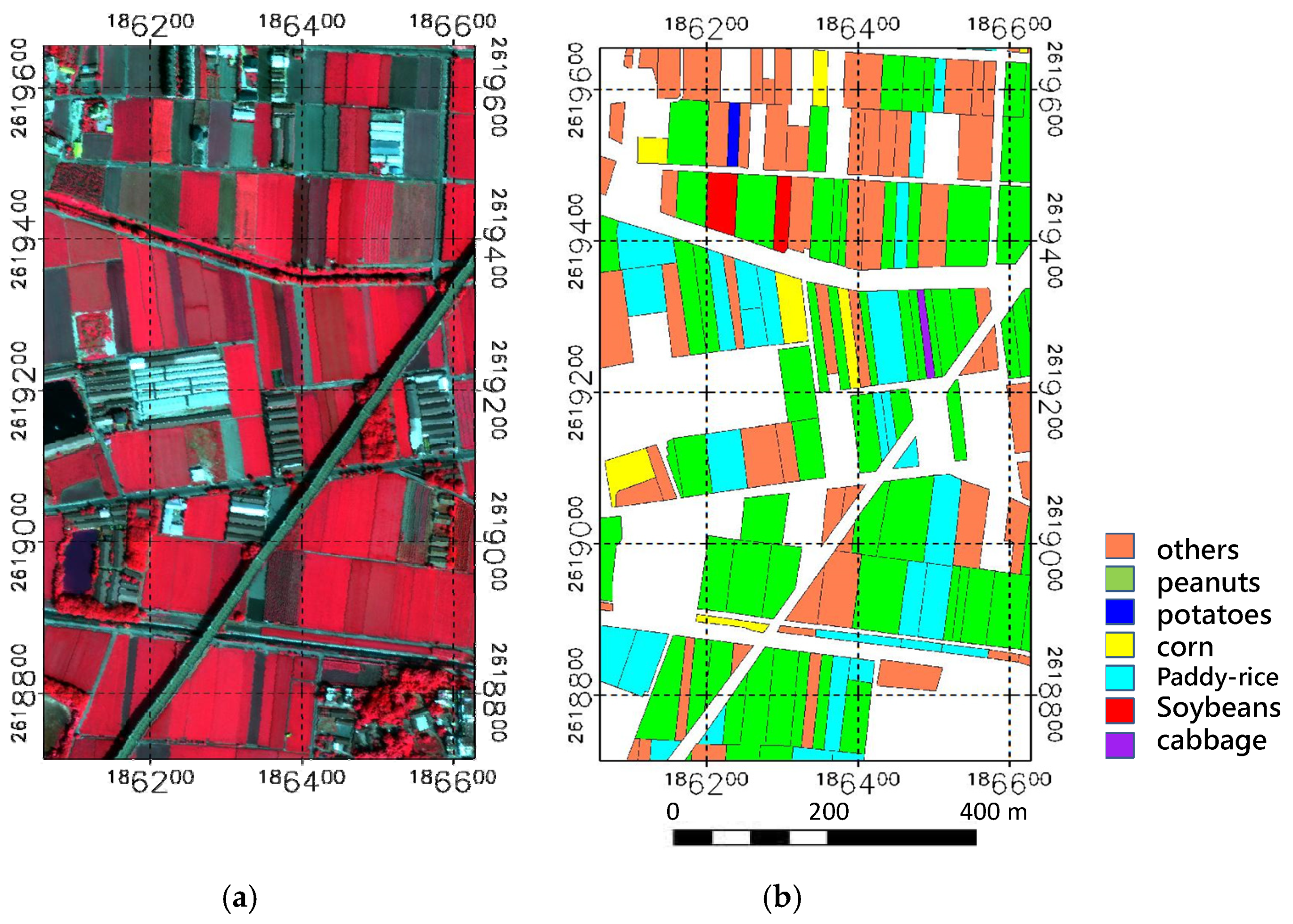
2.1. Brief Introduction on Study Area

The study area is located at Taiwan’s Jianan Plain. It is an important cultivation region designed by the government for different crop productions to display an appropriate size of farmlands. Rice and various vegetables grown on the farmlands are excellent examples for researchers and scientists to study the performance of image classification by using different classifiers and image types. The image data also include non-agricultural land, for example, fishing ponds, buildings, roads, and woodland, with a portion of 39.7% of the total land area (Figure 1). The center coordinates are 186,343′ N, 2,619,185′ E. The experimental area length and width were 0.56 km and 0.94 km. The study area was about 52 hectares.

2.2. Brief Introduction on Image Format

In 2016, the hyperspectral images used in this study were provided by the Compact Airborne Spectrographic Imager (CASI) of the Chung Hsing Surveying Company of Taiwan. The image format has spectral wavelengths ranging from 380 nm to 1050 nm (equivalent to visible to near-infrared light band range), which can obtain up to 288 bands of spectral information [28,29] of 50 cm × 50 cm resolution. Figure 1 presents the study area. After sample creation, 1000 samples were randomly selected for the points by the hyperspectral data, where 500 points were training data, and 500 points were testing data. The 1000 sample points were generated uniformly and randomly in the study area. The rules for multi-objective decision-making were established by considering each different crop as a decision and the 72 bands as attributes. These data were used for the SVM and CNN classifiers. Based on the advantage of measuring instruments after the repeated testing, the bandwidth of 9.6 nm was evenly distributed to the collected spectral data. The bandwidth spacing may cause data noise if re-subdivided again. Therefore, this study took a resolution of 1 m on a hyperspectral image with a total of 72 image bands.

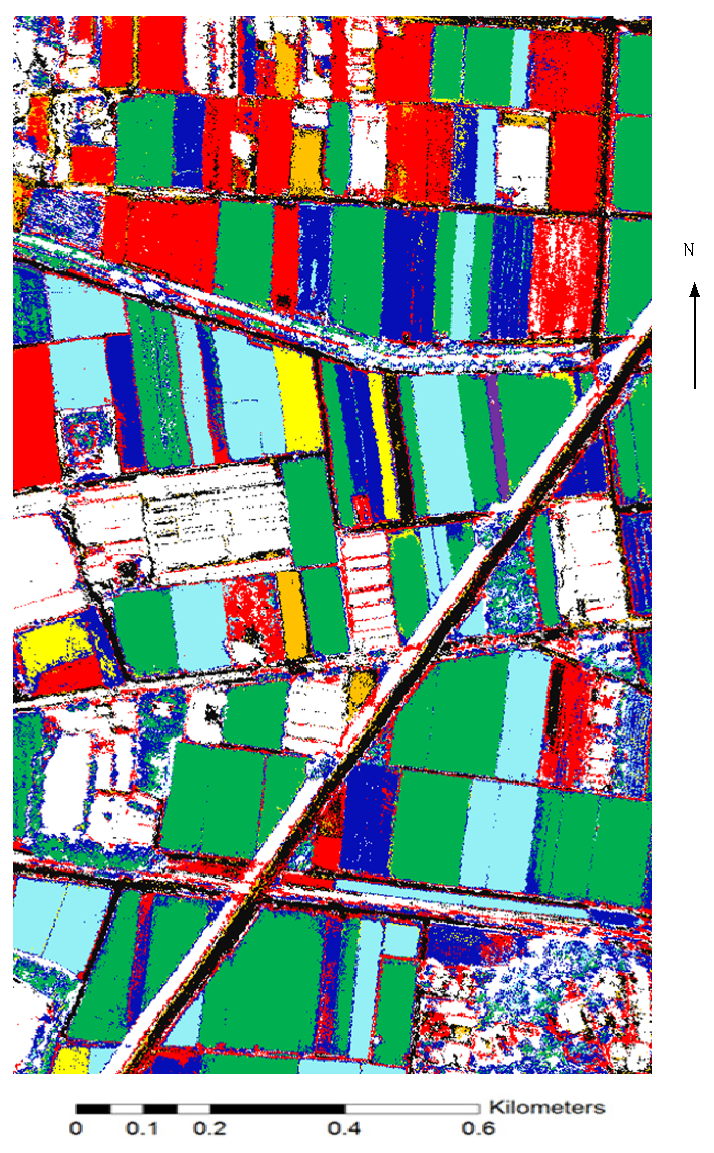
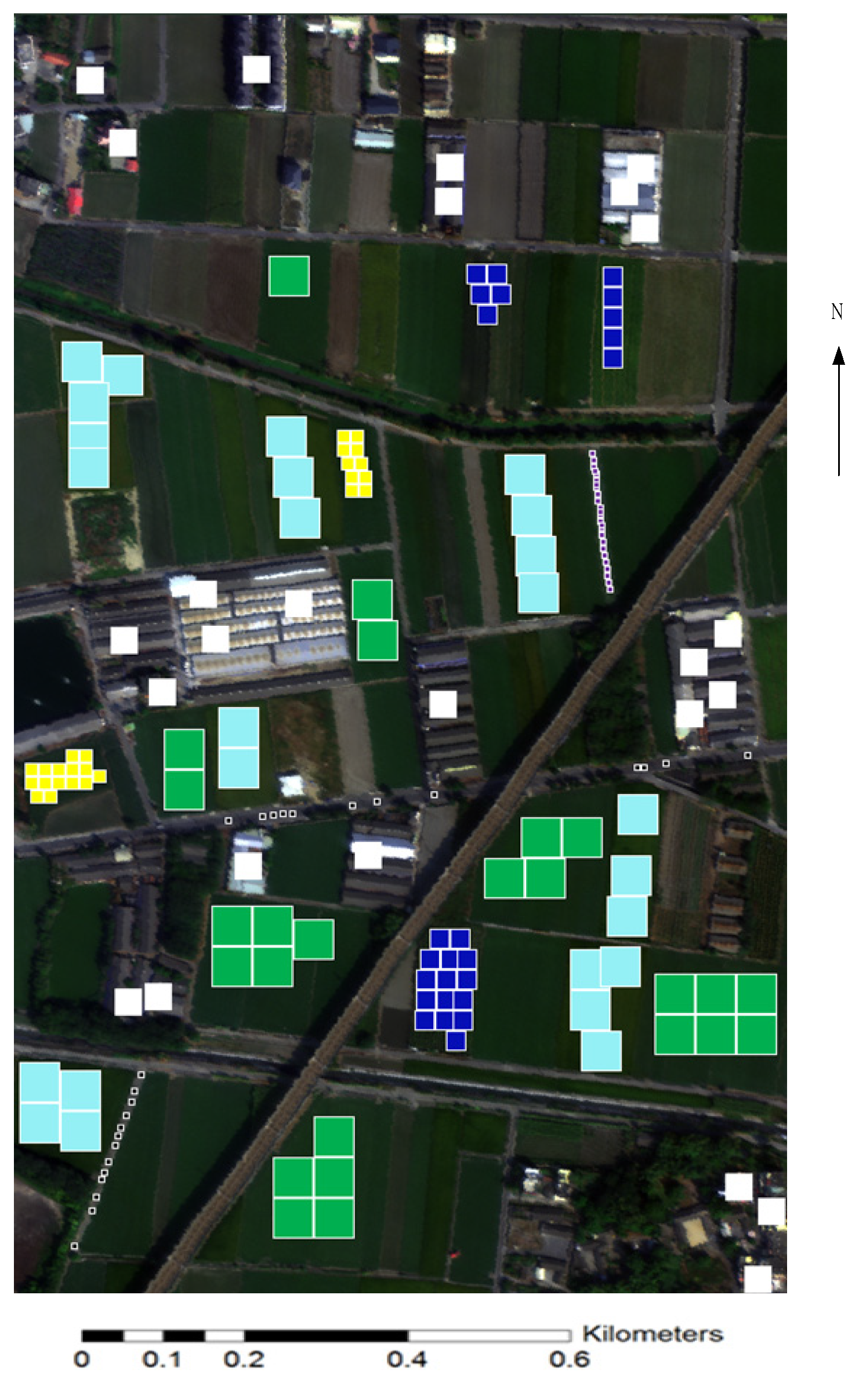
2.3. Image Take Place on Study Area

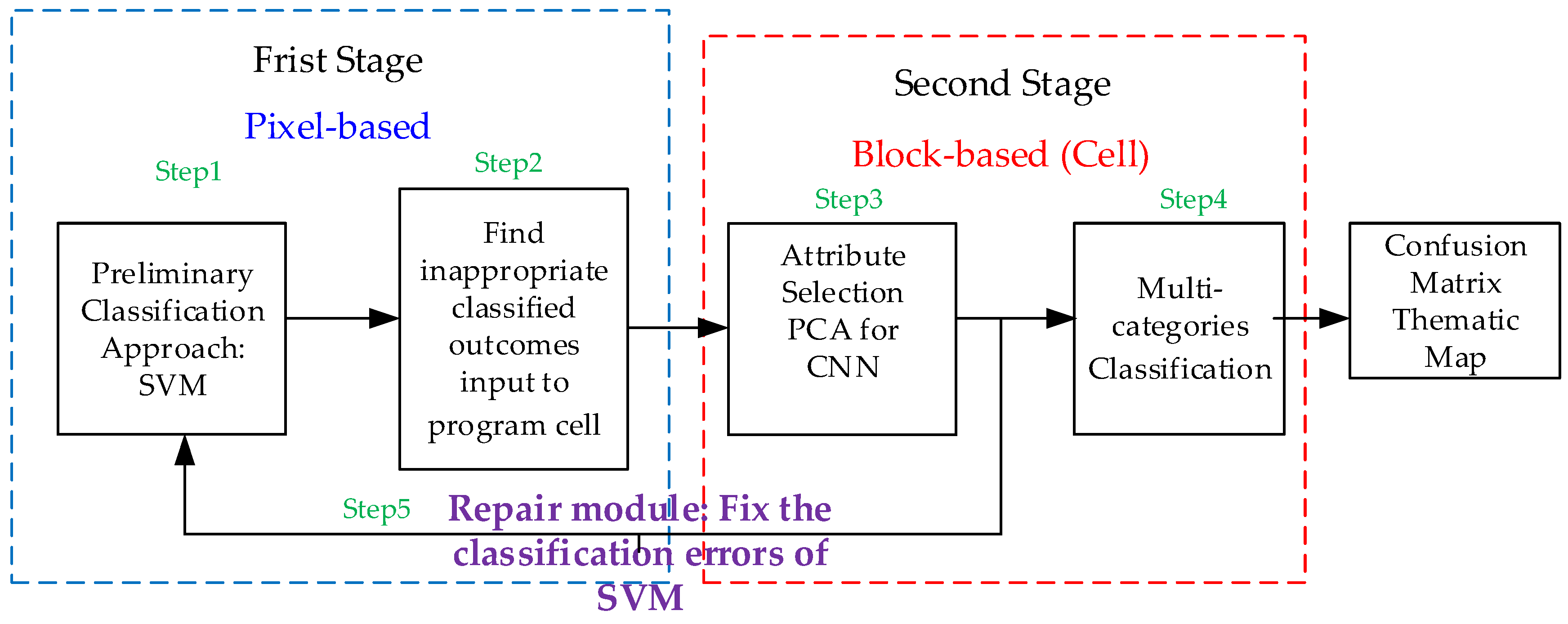
The aerial photo image was taken on 6 April, 2016. The image size was 942 × 569 pixels. This image was already been preprocessed with fusion and standard-calibration [29]. For instance, the leaf pigments and cell walls were hardly absorbed in the near-infrared region (700–1300 nm). The reflectance spectrum of the leaves was quite different in the near-infrared region. In a peak area, the reflectivity is related to various factors such as the thickness, size, arrangement, and cell contents of the mesophyll cells.

The hyperspectral image in this study is shown in Figure 1a. The various distribution of crops and locations are presented in Figure 1b. The image in this study acquired 72 bands with a spectral resolution of 3 nm and a spatial resolution of 1 m. Each band has its own range and color attribute.

3. Research Method

3.1. Study Plan

The research design was broken into two stages. In the first stage, the pixel-based model of the SVM approach was used to analyze the 1000 sample points by the hyperspectral data. Five hundred points of training data and 500 points of testing data were derived from the 1000 sample points. Then, a computer program named cell, which is written in Python, was used to generate the different sizes of blocks to fit the different fields of crops. The Cell program was designed to automatically detect the upper-left corner pixel of different crop fields. Whereas this pixel is determined, the square form of the initial point extends to both x and y directions. Then, it can adjust various sizes of the block to fit different areas of crops. As observed from the remote sensing datasets, convolutional neural networks (CNNs) may be a very appropriate tool to analyze various crop fields due to object classification. The networks are capable of dealing with both detection and classification as neural networks can provide an all-in-one solution for target detection and classification. However, there still exists the need for CNNs of very large ground truth datasets or classification failures that a human eye cannot make. According to this observation, we focused on module solutions, assuming they are provided with a target detection algorithm, which extracts image patches for the recognition and identification stage.

3.2. Support Vector Machine

Support vector machine (SVM) is a superior supervised learning classifier for linear/non-linear classification. The study considers SVM as the concept of improving statistical learning theory. It is also generally applied as an effective classifier to solve many practical problems [12,13,14]. A special feature of these approaches/classifiers is to simultaneously minimize the empirical classification error and maximize the geometric margin. Therefore, it is also known as a maximum margin classifier [11].

Briefly, the concepts of linearly separable classes are the simplest cases for the analysis of three various classes of land-cover. It can be assumed that the training data of k number on samples are presented as $\left\{x_i,y_i\right\}$; where $x\in R^N$ with an N-dimensional space and $y\in \left\{+1,-1\right\}$ is the class label. These training data or patterns are linearly separable if there exists a vector w (determining the orientation of a discriminating plane) and a scalar b (determine the offset of the discriminating plane from the origin) such that

$$y_i\left(w\cdot x_i+b\right)-1\ge 0$$

(1)

The hypothesis space is defined by the set of functions given by:

$$f_{w,b}=sign\left(w\cdot x+b\right)$$

(2)

If the set of examples is linearly separable, the SVM is designed to minimize the value of $\left|\right|w_i\left|\right|$. It is equivalent to also search the segmentation hyperplanes for the distance between the different classes of all of the training data. It also investigates along a line perpendicular to the hyperplane.

This distance is also defined as the margin. The data points are closest to the hyperplane, and are used to determine the position of margin. Accordingly, these given data points are called support vectors. Thus, the number of support vectors needs to be as small as possible.

The problem of minimizing $\left|\right|w_i\left|\right|$ is solved by applying standard quadratic programming (QP) optimization techniques. It also transforms the problem to a dual space by using Lagrangian multipliers. The Lagrangian is presented by introducing positive Lagrange multipliers ${\lambda }_i, i=1,\dots k$. The solution to the optimization problem is attained by considering the saddle point of the Lagrange function

$$\begin{array}{c}L\left(w,b,\lambda \right)=\frac{1}{2}{\Vert w\Vert }^2-{\displaystyle \sum _{i=1}^k{\lambda }_i{y}_i\left(w\cdot x_i+b\right)+{\displaystyle \sum _{i=1}^k{\lambda }_i}}\end{array}$$

(3)

The solution in Equation (5) is described in which the L(w, b, $\lambda$) is minimized with respect to w and b and maximized corresponding to ${\lambda }_i\ge 0$. Therefore, for a two-class problem, the decision rule successfully cuts the two classes, which can be written as:

$$f\left(x\right)=sign\left({\displaystyle \sum _{i=1}^k{\lambda }_i{y}_i\left(x\cdot x_i\right)+b}\right)$$

(4)

Soft margin formulation was employed to classify linearly inseparable data by Cortes and Vapnik (1995). More specifically, if there is no specific linear decision boundary that can perfectly separate the data, this is so-called linearly inseparable. They proposed that the restriction of each training vector of a given class us on the same side of the optimal hyperplane that applies the value. In ξ_i ≥ 0, the SVM algorithm for the hyperplane maximizes the margin. ξ_i is the count of errors made by our classifier on the set of training examples. Meanwhile, it minimizes the quantity of proportional samples to the number of misclassification errors. This trade-off function is negotiated with the margin and misclassification error that is also governed by a positive constant C such as in terms of $\infty >\mathrm{C}>0$. Thus, for non-separable data, Equation (6) can be written as:

$$L\left(w,b,\lambda ,\xi ,\mu \right)=\frac{1}{2}{\Vert w\Vert }^2+C{\displaystyle \sum _i{\xi }_i-}{\displaystyle \sum _i{\lambda }_i\left\{y_i\left(w\cdot x_i+b\right)-1+{\xi }_i\right\}-{\displaystyle \sum _i{\mu }_i{\xi }_i}}$$

(5)

where μ_i is the Lagrange multiplier to enforce the ξ_i to be positive. The solution of Equation (5) is determined by the saddle points of the Lagrangian by minimizing with respect to w, x, and b, and maximizing with respect to ξ_i ≥ 0 and μ_i ≥ 0. A computer program written in Python was used analyze the SVM approach. Later, the first stage of the SVM results is presented.

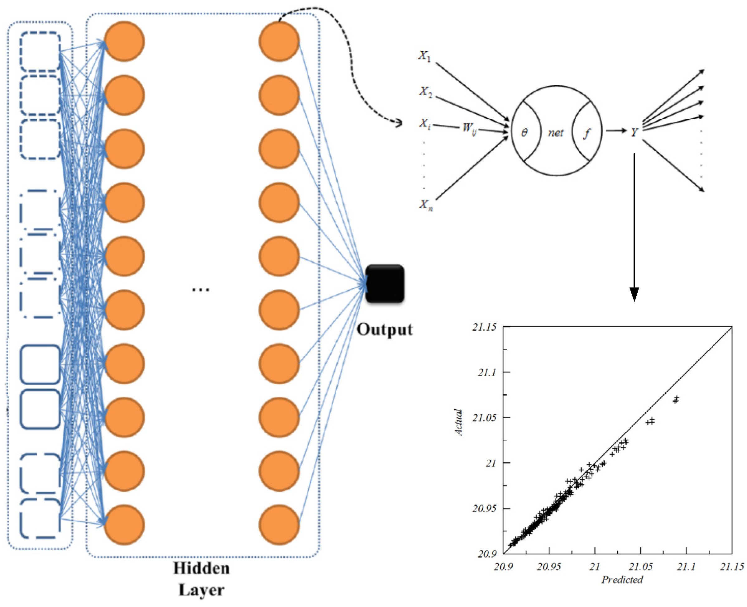
3.3. Deep Learning for Regional Image Classification

A wide new application in deep learning has been developed in recent years, especially the convolutional neural network (CNN) [18]. This sort of artificial neural network has been exploited quickly to provide excellent outcomes in various domains. They can adaptively learn the spatial difference in hierarchies of features through backpropagation by using multiple building blocks of convolution layers, pooling layers, fully connected layers, etc. Most CNN-based applications for object recognition and detection have been successfully developed for optical images to solve unpredictable/uncountable objects [19]. If other imaging sensors (radar, sonar, and infrared) are employed, difficulties may be encountered on having a better understanding of the intrinsic image characteristics. Hence, CNNs have been successfully used for the classification of ground targets in many types of remote sensing imagery. Some CNNs have already been proposed for this kind of image for target classification [18,19]. They surpass previous shallow machine learning techniques in image classification tasks. It could also be adapted to work on other computer vision problems such as pose estimation, super-resolution, or image segmentation [23,24,25]. Figure 2 presents an overall structure of the network and a global average pooling operation by the softmax layer. It also automatically evaluates the errors among the true values and the predicted values.

3.3.1. Convolution

When the program processes the images or identifies them, it needs to take the characteristics/features of the graph from each pixel. In addition to the value of each pixel, it needs to consider the different connections among pixels and pixels. One way to characterize the image is to filter the image to obtain more useful information such as using the edge (Edge Detection) detection of the derivative (mask). In other words, convolutional layers are strong feature extractors in which the convolutional filters are capable of finding the features of images. Hence, each convolutional neuron processes data that are responsible for its receptive field. The fully connected feedforward neural networks are often used to learn features as a set of classified data. However, it is not practical to apply this architecture to images. Hence, a very high number of neurons is taken into consideration even in shallow (opposite of deep) architecture. Through using a very large input size of pixels associated with images, those pixels may be considered as a relevant variable. That is, the convolution operation brings a new solution to this problem as it reduces the number of free parameters and allows the network to be deeper with using fewer parameters. The usage of convolution achieves the function of filtering the image to obtain only the edge of the picture.

3.3.2. Max-Pooling

Pooling is another important concept in processing the convolutional neural networks, which is a form of sampling [25,26,27]. There are many different forms of nonlinear pooling, in which max-pooling is the most common. The max-pooling concept is to apply the maximum value from each of a cluster of neurons at the prior layer. The image of the inputs is divided into many rectangular areas with maximum outputs for each sub-area to facilitate the calculation of pooling. This mechanism is effective for detecting a feature and its precise position is far less important than its relative position with other features. The pooled layer progress continuously to decrease the spatial size of the data [28]. Then, the number of parameters and the number of calculations is also reduced simultaneously, which to some extent governs the overfitting problems [29].

3.3.3. Colorful Image

The computer hardware encounters two problems in dealing with colorful images [30,31]:

(3.1) Requires a lot of memory. For instance, for a color picture with dimensions of 30 × 30, it needs to use 30 × 30 × 24 input neurons. If the hidden layer in the middle is constructed with 100 neurons, each neuron needs a weight value of floating points (8 bytes). Then, a total amount of 21,600 × 100 × 8 = 0.14648 GB is the request memory.

(3.2) Multi-layer perceptron only determines every single pixel in the picture, which completely abandons crucial image features. When the human eye sees the patterns of the object, it also makes individual judgments/feature about the characteristics of different parts of this object. However, multi-layer sensors do not take advantage of these features. Thus, the accuracy in the interpretation of the image may not be as good as CNN. Eventually, while the computing convolutional and max-pooling layers are undertaken, the high-level reasoning in the neural network is done via fully connected layers. Hence, many neurons in a fully connected layer are successfully connected to all actions in the previous layer [32,33,34].

3.3.4. Determination of Layers

In a convolutional neural network, there are three sorts of layers: the convolutional layer, pooling layer, and fully connected layer. Each of these layers has different parameters that can be optimized and performs a different task on the input data. The initial layer number is determined similarly to ANN. The number of layers and the number of nodes in each layer are model hyper-parameters, which need to be specified in the developed program. All of the classification answers will come back to the need for careful experimentation of all layers to work best for the provided specific dataset.

In this study, a computer program written in Python was used to carry out the analysis of the CNN approach. The outcomes will be used as the second stage of the results.

3.4. Study Plan

The whole research plan was broken into five steps (see Figure 3): (1) Support vector machine before processing; (2) material preparation for PCA attribute selection; (3) convolutional neural network reprocessing detail class; (4) establish multi-classification and layer rules, and (5) execute the repair module to fix the error classification outcomes. It can be summarized as follows:

Figure 4 presents the progress on how does the Cell program works. First, it was developed to select a paddy rice area as an example. Figure 4a shows how the regional object classification model (ROC) [32] selects a combination set of parameters of the seeds of Area (A) and Similarity (S). Second, the red line is the linear regression function by collecting the coordinate data of blue pixels that are generated from the ROC model and gradually increases to the surrounding levees for each margin of the sides to the whole integrated patch. These two parameters are adjusted to enlarge and merge different cells as one region. In addition, the program automatically detects tiny parts of the region and also removes them. The final outcome is shown in Figure 4b.

4. Discussion of the Results

4.1. First Stage Analysis of Support Vector Machine (SVM)

Table 1. Training samples and testing samples of labels and colors.

Category	Training Samples	Testing Samples	Color
Cabbage	25	75
Empty ground	55	94
Corn	45	132
Road	149	435
Building	152	408
Uncultivated land	114	325
Potatoes	119	273
Paddy rice	143	404
Peanuts	251	725

presents the number of training samples and testing samples. All of these samples were randomly and uniformly selected for each different category. It also presents, by different colors, the various crops, buildings, and roads. The training samples were used to construct the SVM model. The testing samples were employed for the validation efficiency of the SVM model. Specifically, the functions of the support vector machine can be divided into four types: linear functions, polynomial functions, radial basis functions, and S functions. The user selects the core function by considering the appropriate conditions. The parameters are adjusted for different kernel functions that are also different. The user has to adjust the kernel function and parameters according to the situation, which will have a significant impact on the prediction accuracy rate. More specifically, different distribution and dimension of data may search for a proper kernel function. In the meantime, the initial value of the parameter may also influence the computation speed. In this study, the radial basis function kernel (RBF) was selected for calculation. To obtain better model parameters, the grid search method repeats the test parameters C = 2100 (penalty parameter) and g = 2 (gamma function) for possible combinations and calculates the correct rate of its parameters (C, g). If it meets its condition, stop the repeated test and output its best C and g parameters, otherwise re-substitute with the new parameters until the optimal combinations are found.

This step is to optimize the model by searching for a proper solution of the classification outcomes in the previous step. The testing data for the unknown result is substituted into the classification model constructed by the previous step and the obtained results are aggregated in which the overall classification accuracy rate is calculated to perform the evaluation. It explores the effectiveness of machine learning under its selection points and different attribute data. The accuracy assessment of this study was divided into two parts: (1) the thematic map, and (2) the error matrix. Figure 5 presents the thematic map of the classification outcomes of SVM. There are still some misjudgments that need to be improved.

Table 2. The confusion matrix of various data by the support vector machine (SVM) approach.

presents the confusion matrix of the results of the SVM. It is noted that the building, road, and uncultivated land are the “others” listed in Figure 1b.

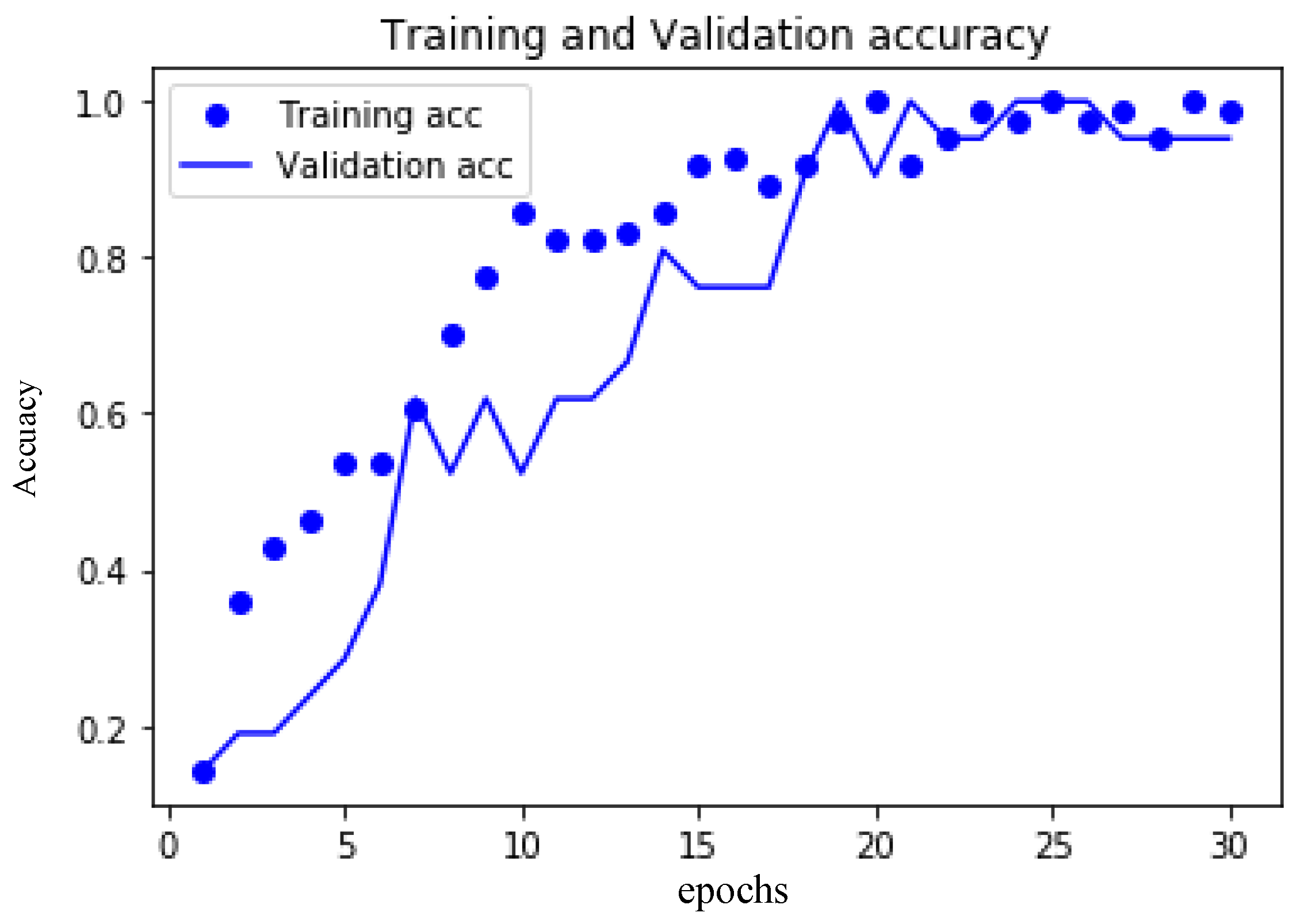
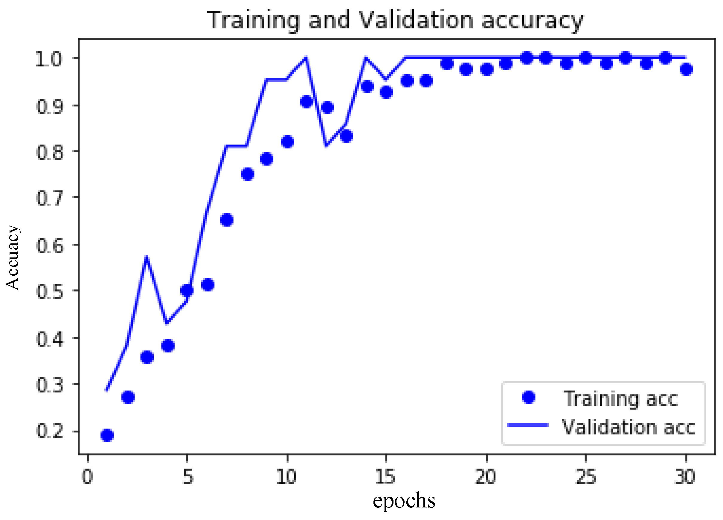
4.2. Second Stage: Improvement Classification of CNN

The study provides nine categories divided into nine classes for the analyzed data of the CNN. Various cell sizes were generated to fit the crop size considering the inputs for CNN. Thus, the regional object classification (ROC) model [32,33] promotes the image information from the pixel-scale to the regional-scale (blocks or cells) by operating units to establish crop information. The information scale from pixel to a regional area needs a program to be written to display the needs of each crop area and was also identified for different crop analyses.

As part of this study, the study employed PCA as a feature extraction tool [33,34] for the different components to approach accuracy. A fundamental question arises: “how many requested dimensions are needed when the PCA is executed?” Hence, it was decided that in order to have a better understanding of how many PCAs were enough to carry out the outcomes of this study, the process of PCA took 8, 16, and 24 three different combinations to access the accuracy. It automatically detected the edge of each size of different farms concerning various crops. The program was designed to make a 30 × 30 CNN model and display different combination outcomes as results. For instance,

Table 3. Outputs for CNN model of sequential_14. (Model: “sequential_14” with kernel size 3 × 3 of original size 30 × 30).

Layer	Output Feature Map	Kernel Size	Output Size
Conv1	150	3 × 3	28 × 28
Max pool 2 × 2			14 × 14
Conv2	100	3 × 3	12 × 12
Max pool 2 × 2			6 × 6
Conv3	150	3 × 3	4 × 4
softmax			7 × 1

shows the outputs of sequential_14. The original size was 30 × 30. Layer 1 switched to 28 × 28. The activation function of the CNN model was “Relu”. The maximum epoch number was set up as 100 with a validation split of 0.2. After executing Maxpool 2 × 2, it was reduced to 14 × 14… and so on. Then, the program automatically calculated softmax 7 × 1, in which it will transform into a one-dimensional array.

The largest size was a 30 × 30 square and the smallest was a 5 × 5 square. As the ROC program is conducted, the Cell program is then used to compute the square area of the crop area. The Cell program will automatically detect the appropriate size of each crop to attain different moving size windows. Figure 6 displays the different sizes of the samples in region-based classification. Since different crops have different sizes, the region-based classification program was executed by the Cell program as aforementioned in Figure 4. It is step-by-step used to detect the different areas of the entire image. Those samples were selected for the CNN model to analyze the classification accuracy.

Table 4. The cell-size of the CNN model.

Class	Training Samples	Testing Samples	Size	Conv. Resize
Cabbage	15	10	5 × 5	30 × 30
Corn	15	10	10 × 10	30 × 30
Road	15	10	20 × 20	30 × 30
Building	15	10	5 × 5	30 × 30
Potatoes	15	10	15 × 15	30 × 30
Paddy rice	15	10	30 × 30	30 × 30
Peanuts	15	10	30 × 30	30 × 30

presents the size of the cell on the CNN model, which obeys various max sizes of crop fields in the observations [32,33]. The location of the cells is displayed in Figure 6.

Table 5. Confusion matrix of CNN by principle component analysis (PCA) 8 epoch 30.

	Paddy	Peanuts	Potatoes	Corn	Cabbage	Road	Building
Paddy	10	0	0	0	0	0	0	100%
Peanuts	0	10	0	0	0	0	0	100%
Potatoes	0	2	8	0	0	0	0	80%
Corn	0	0	0	10	0	0	0	100%
Cabbage	0	0	0	0	10	0	0	100%
Road	0	0	0	0	0	10	0	100%
Building	0	0	0	0	0	0	10	100%
	100%	83.3%	100%	100%	100%	100%	100%

shows the confusion matrix of CNN by PCA selection of PCA1, PCA2, PCA3 to PCA8. The study decides to select the number of epochs which equals 30. It is found that only the potato fields have two misjudgments by omission error. The accuracy rate is 97.1%.

Figure 7 presents the convergence of PCA = 8 of 30 epochs. The x-axis is the epoch number and the y-axis is the predicted accuracy. The dot represents the accuracy of the training data with respect to different epochs. The line is the testing data with respect to different epochs.

Table 5 shows the confusion matrix of CNN by PCA selection of PCA1, PCA2, PCA3… to PCA24. Epochs equal to 30 were used as criteria to observe the difference in accuracy. The cabbage fields had only one misjudgment by omission error. The accuracy rate was 98.6%. We then used potatoes as an example to explain how the repair module worked.

Figure 8 presents the convergence of PCA = 24 of 30 epochs. The x-axis is the epoch number. The y-axis is the predicted accuracy. The dot represents the accuracy of the training data concerning different epochs. Compared to Figure 7, the convergence rate moved faster than that of PCA = 8. It almost varied smoothly when the epoch = 15 or greater. However, PCA = 8 needed 22 epochs to perform a stable result. In other words, through a series of testing, this study found that CNN performed well for a certain number of PCA features to approach a satisfactory accuracy rate [34,35,36]. The line was the testing data for different epochs.

Table 6. Confusion matrix of CNN by PCA 24 epoch 30.

presents the outcomes of different PCA on feature selection. It can be observed that while PCA = 8, the accuracy of RBF-based SVM was 94.95% of the accuracy. When increasing the number of PCA, the accuracy increased slightly. Unfortunately, the accuracy rate still could not reach 100%. This was produced by a huge number of pixels causing pixel-based classification errors (salt-pepper effects), especially on a high-resolution image. Accordingly, the repair module is designed to eliminate the false classification made by SVM.

To further explain how the repair module works, an example was used to perform its superiority. For instance, potatoes in the SVM classification output was the worst case compared with the accuracy of all other predictions (Table 2). Fortunately, the CNN model by PCA 24 epoch 30 had 100% of accuracy for potatoes (see Table 6). Since the CNN model is a regional-based classification, it renders an appropriate solution in classification. The repair module was obtained by the CNN of block-based (Cell) data (see

Table 7. The classification outcomes of SVM and SVM + CNN.

Categories	PCA = 8	PCA = 16	PCA = 24	Full-Band (Bands = 72)
SVM with RBF	94.95%	95.16%	95.51%	95.85%
CNN Accuracy	Epoch = 30 97.1%	Epoch = 30 98%	Epoch = 30 98.6%	Epoch = 100 100%
* SVM + CNN Repair module	100%	100%	100%

* Repair module will fix the inappropriate classification outcomes of SVM (see Figure 4).

). Most of those errors were produced by salt-pepper effects through SVM analysis. The repair module successfully removed these errors. In addition, the computation of full-band image data (72 bands) took 145 times more computational time than that of PCA = 8. If used in the repair module, a huge amount of computational time can also be saved.

Since the CNN approach had a better result than SVM, a fundamental question arises: Why not directly use the CNN model?

Table 8. The classification outcomes of SVM and SVM + CNN.

Categories	PCA = 8	PCA = 16	PCA = 24	Full-Band (Bands = 72)
SVM with RBF	0.5 min	1.7 min	3.4 min	1.3 h
CNN Accuracy	3.1 min	8.2 min	15.2 min	4 h
* SVM + CNN Repair module	3.6 min	10 min	18.7 min	5.3 h
Accuracy	100%	100%	100%	100%

* Repair module will fix the inappropriate classification outcomes of SVM (see Figure 4).

presents the efficiency of computational time. The testing computer hardware was i7-8700 with 16 RAM and a 4G GTX-1050 video Ccard with the calculation of the entire thematic map. The operating system was Win10 using the Python package of Keras in TensorFlow.

With the same level of accuracy, the repair module in the two-stage of classification of our study provided a superior solution in computation time. A full band needs more than five hours to attain the same level of 100% accuracy. However, PCA = 8 with the SVM + CNN repair module can approach the same level of accuracy in 3.6 min. Consequently, this study provides a brilliant idea to the effectiveness of our two-stage model by adding a repair-module.

5. Summary and Conclusions

The analysis, measurement, and computation of remote sensing images often require an enhanced computation model to combine classifiers to approach a good result. If different classifiers can be integrated to obtain a better outcome, it would be feasible to combine them by considering each of the advantages of the feature on various classifiers. Hence, the study developed an integrated image classification crop system to classify multiple major crops in the Chiayi Golden Corridor in a multi-objective decision-making system. The CASI hyperspectral remote sensing image data were used in this study. The plan was to use the hyperspectral data and two-stage classification to construct multi-class classification with support vector machine + convolutional neural network and design parallel research for batch processing.

(a)

The first stage: The SVM approach was carried out for the roughly pixel-based results. The accuracy rate was about 95.85%.

(b)

The second stage: The deep learning method was carried out for cell-based results. Three different cases were considered: PCA = 8, epoch = 30, the accuracy was 97.1%; PCA = 16, epoch = 30, where the accuracy was 98%; and PCA = 24, epoch = 30, where the accuracy was 98.6%.

(c)

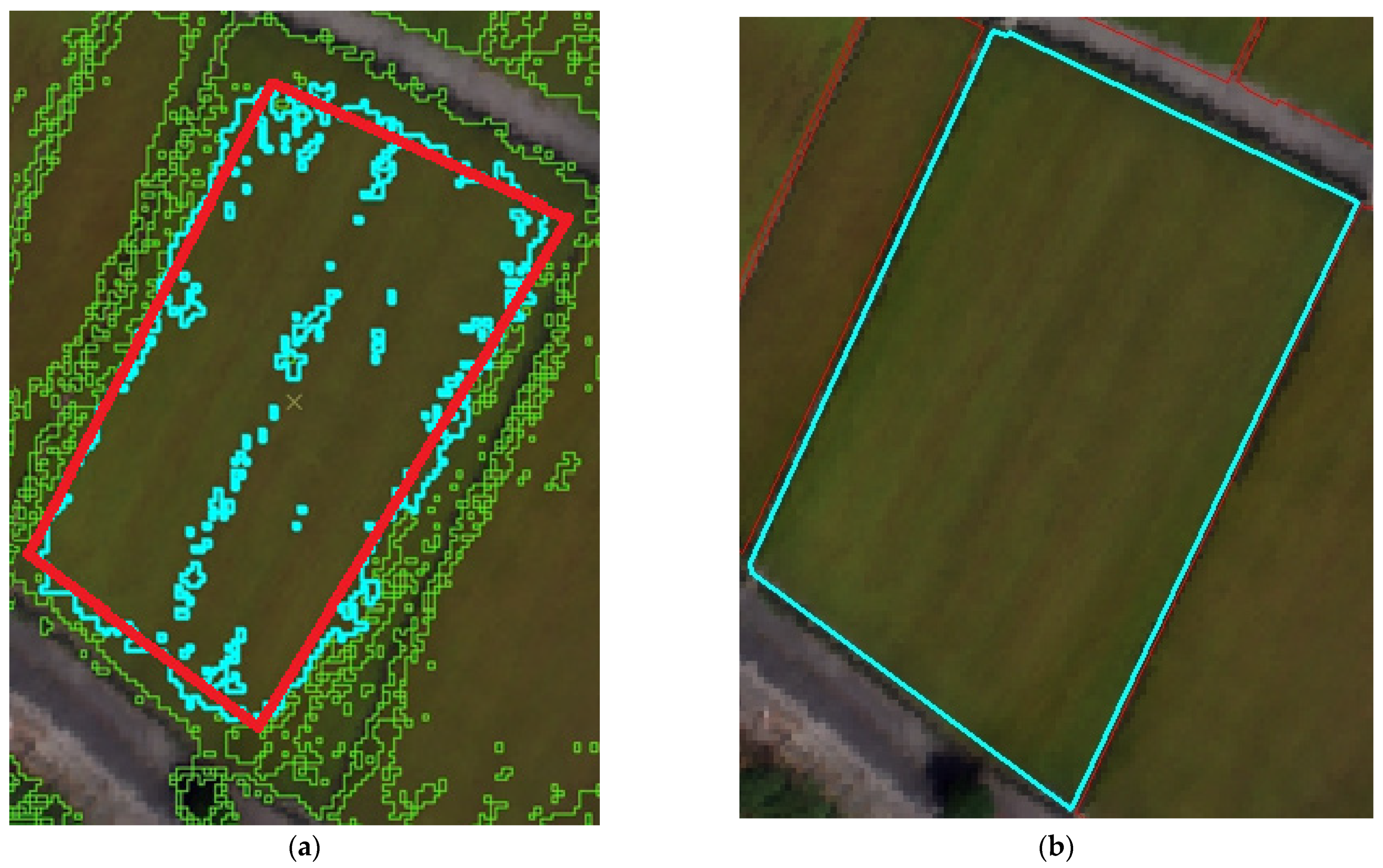
The repair module was designed to use the CNN classification outcomes to fix the pixel-based model of SVM classification errors. The target cell also successfully eliminated the salt and pepper effect.

It is noteworthy that the same improvements could also be applied in a similar study area in the following condition. If the dataset has different regions with various sizes of crops, it could be of help to apply this approach. On the other hand, other studies with serious salt and pepper effect can also use this two-stage method. A comparison was made by considering four major crops, buildings, and roads for deep learning. In this study, the pros of the support vector machine (SVM) for hyperspectral image classification can obtain an initial relative good result and deep learning (convolution neural network; CNN) with the developed repair module can also improve the classification of image details.

References

1. Wan, S.; Wang, Y.P. The comparison of density-based clustering approach among different machine learning models on paddy rice image classification of multispectral and hyperspectral image data. Agriculture 2020, 10, 465. [Google Scholar] [CrossRef]
2. Lu, D.; Mausel, P.; Batistella, M. Land-Cover binary change detection methods for use in the moist tropical region of the Amazon: A comparative study. Int. J. Remote Sens. 2005, 26, 101–114. [Google Scholar] [CrossRef]
3. Cao, J.; Leng, W.; Liu, K.; Liu, L.; He, Z.; Zhu, Y. Object-Based mangrove species classification using unmanned aerial vehicle hyperspectral images and digital surface models. Remote Sens. 2018, 10, 89. [Google Scholar] [CrossRef] [Green Version]
4. Cheriyadat, A.; Bruce, L.M. Why principal component analysis is not an appropriate feature extraction method for hyperspectral data. Geosci. Remote Sens. Symp. 2003, 104, 3420–3422. [Google Scholar]
5. Muhammed, H.H. Hyperspectral crop reflectance data for characterising and estimating fungal disease severity in wheat. Biosyst. Eng. 2005, 91, 9–20. [Google Scholar] [CrossRef]
6. Lei, T.C.; Wan, S.; Wu, S.C.; Wang, H.P. A new approach of ensemble learning technique to resolve the uncertainties of paddy area through image classification. Remote Sens. 2020, 12, 3666. [Google Scholar] [CrossRef]
7. Bertels, L.; Vanderstraete, T.; Van Coillie, S. Mapping of coral reefs using hyperspectral CASI data; a case study: Fordata, Tanimbar, Indonesia. Int. J. Remote Sens. 2008, 29, 2359–2391. [Google Scholar] [CrossRef]
8. Nguyen, A.; Yosinski, J.; Clune, J. Deep neural networks are easily fooled: High confidence predictions for unrecognizable images. In Proceedings of the IEEE Conference on Computer Vision and Pattern Recognition, Boston, MA, USA, 7–12 June 2015; pp. 427–436. [Google Scholar]
9. Rodarmel, C.; Shan, J. Principal component analysis for hyperspectral image classification. Surv. Land Inf. Sci. 2002, 62, 115–122. [Google Scholar]
10. Tuia, D.; Pasolli, E.; Emery, W.J. Using active learning to adapt remote sensing image classifiers. Remote Sens. Environ. 2011, 115, 2232–2242. [Google Scholar] [CrossRef]
11. Wan, S.; Chang, S.H. Crop classification with WorldView-2 imagery using support vector machine comparing texture analysis approaches and grey relational analysis in Jianan Plain, Taiwan. Int. J. Remote Sens. 2019, 40, 8076–8092. [Google Scholar] [CrossRef]
12. Du, P.J.; Tan, K.; Xing, X.S. A novel binary tree support vector machine for hyperspectral remote sensing image classification. Opt. Commun. 2012, 285, 3054–3060. [Google Scholar] [CrossRef]
13. Chapelle, O.; Haffner, P. Support vector machines for histogram-based image classification. VN Vapnik—IEEE Trans. Neural Netw. 1999, 10, 1055–1064. [Google Scholar] [CrossRef]
14. Wan, S.; Lei, T.C.; Ma, H.L.; Cheng, R.W. The analysis on similarity of spectrum analysis of landslide and bareland through hyper-spectrum image bands. Water 2019, 11, 2414. [Google Scholar] [CrossRef] [Green Version]
15. Pradhan, B. A comparative study on the predictive ability of the decision tree, support vector machine and neuro-fuzzy models in landslide susceptibility mapping using GIS. Comput. Geosci. 2013, 51, 350–365. [Google Scholar] [CrossRef]
16. Foody, M.G.; Mathur, A. A relative evaluation of multiclass image classification by support vector machines. IEEE Trans. Geosci. Remote Sens. 2004, 42, 1335–1343. [Google Scholar] [CrossRef] [Green Version]
17. Furey, T.; Cristianini, N.; Duffy, N.; Bednarski, D.; Schummer, M.; Haussler, D. Support vector machine classification and validation of cancer tissue samples using microarray expression data. Bioinformatics 2000, 16, 906–914. [Google Scholar] [CrossRef] [PubMed]
18. Kim, S.; Song, W.J.; Kim, S.H. Infrared variation optimized deep convolutional neural network for robust automatic ground target recognition. In Proceedings of the IEEE Computer Society Conference on Computer Vision and Pattern Recognition Workshops, Honolulu, HI, USA, 21–26 July 2017; pp. 195–202. [Google Scholar]
19. Acharya, U.R.; Oh, S.L.; Hagiwara, Y.; Tan, J.H.; Adeli, H. Deep convolutional neural network for the automated detection and diagnosis of seizure using EEG signals. Comput. Biol. Med. 2018, 100, 270–278. [Google Scholar] [CrossRef]
20. Zhou, Q.; Flores, A.; Glenn, N.F.; Walters, R.; Han, B. A machine learning approach to estimation of downward solar radiation from satellite-derived data products: An application over a semi-arid ecosystem in the U.S. PLoS ONE 2017, 12, e0180239. [Google Scholar] [CrossRef] [Green Version]
21. Blei, D.M.; Ng, A.Y.; Jordan, M.I. Latent dirichlet allocation. J. Mach. Learn. Res. 2003, 3, 993–1022. [Google Scholar]
22. Senthilnath, J.; Omkar, S.N.; Mani, V. Crop Stage Classification of Hyperspectral Data Using Unsupervised Techniques. IEEE J. Sel. Top. Appl. Earth Obs. Remote Sens. 2013, 6, 861–866. [Google Scholar] [CrossRef]
23. Pang, Y.; Sun, M.; Jiang, X. Convolution in convolution for network in network. IEEE Trans. Neural Netw. Learn. Syst. 2018, 29, 1587–1597. [Google Scholar] [CrossRef] [Green Version]
24. Yu, S.; Jia, S.; Xu, C. Convolutional neural networks for hyperspectral image classification. Neurocomputing 2017, 219, 88–98. [Google Scholar] [CrossRef]
25. Krizhevsky, A.; Sutskever, I.; Hinton, G.E. ImageNet classification with deep convolutional neural networks. Commun. ACM 2017, 60, 84–90. [Google Scholar] [CrossRef]
26. Zhang, C.; Sargent, I.; Pan, X.; Li, H.; Gardiner, A.; Hare, J.; Atkinson, P.M. An object-based convolutional neural network (OCNN) for urban land use classification. Remote Sens. Environ. 2018, 216, 57–70. [Google Scholar] [CrossRef] [Green Version]
27. Wu, Q.; Gao, T.; Lai, Z.; Li, D. Hybrid SVM-CNN classification technique for human–vehicle targets in an automotive LFMCW radar. Sensors 2020, 20, 3504. [Google Scholar] [CrossRef] [PubMed]
28. Lee, H.; Kwon, H. Going deeper with contextual CNN for hyperspectral image classification. IEEE Trans. Image Process. 2017, 26, 4843–4855. [Google Scholar] [CrossRef] [PubMed] [Green Version]
29. Guo, Y.; Liu, Y.; Oerlemans, A.; Lao, S.; Wu, S.; Lew, M.S. Deep learning for visual understanding: A review. Neurocomputing 2016, 187, 27–48. [Google Scholar] [CrossRef]
30. Espindola, G.M.; Camara, G.; Reis, I.A.; Bins, L.S.; Monteiro, A.M. Parameter selection for region-growing image segmentation algorithms using spatial autocorrelation. Int. J. Remote Sens. 2006, 27, 3035–3040. [Google Scholar] [CrossRef]
31. Gong, Y.H. Advancing content-based image retrieval by exploiting image color and region features. Multimed. Syst. 1999, 7, 449–457. [Google Scholar] [CrossRef]
32. Wan, S.; Lei, T.C.; Chou, T.Y. Optimized object-based image classification: A development of landslide knowledge decision support system. Arab. J. Geosci. 2014, 7, 2059–2070. [Google Scholar] [CrossRef]
33. Lu, H.; Ma, L.; Fu, X.; Liu, C.; Wang, Z.; Tang, M.; Li, N. Landslides information extraction using object-oriented image analysis paradigm based on deep learning and transfer learning. Remote Sens. 2020, 12, 752. [Google Scholar] [CrossRef] [Green Version]
34. Narendra, G.; Sivakumar, D. Deep learning based hyperspectral image analysis-a survey. J. Comput. Theor. Nanosci. 2019, 16, 1528–1535. [Google Scholar] [CrossRef]
35. Prasad, S.; Bruce, L.M. Limitations of principal components analysis for hyperspectral target recognition. IEEE Geosci. Remote Sens. Lett. 2008, 5, 625–629. [Google Scholar] [CrossRef]
36. Ball, J.E.; Anderson, D.T.; Chan, C.S. Comprehensive survey of deep learning in remote sensing: Theories, tools, and challenges for the community. J. Appl. Remote Sens. 2017, 11, 1. [Google Scholar] [CrossRef] [Green Version]
Figure 1. Study area. (a) Hyperspectrum image (April, 2016). (b) Ground truth data.
Ijgi 10 00242 g001
Figure 2. The convolutional neural network (CNN) model for prediction.
Ijgi 10 00242 g002
Figure 3. Research steps of the study.
Ijgi 10 00242 g003
Figure 4. The progress of the Cell program derived from the regional object classification model (ROC) program. The line is represent the margin of linear regression function by collecting the coordinate data of blue pixels: (a) The ROC program find seeds of Area and Similarity. (b) Removal of the tiny parts to be integrated.
Ijgi 10 00242 g004
Figure 5. Thematic map of the first stage on SVM.
Ijgi 10 00242 g005
Figure 6. Resize window of CNN selection by the Cell program and the prepared inputs for CNN.
Ijgi 10 00242 g006
Figure 7. Accuracy of feature selection of PCA 8 epoch 30.
Ijgi 10 00242 g007
Figure 8. Accuracy of feature selection of PCA 24 of epoch 30.
Ijgi 10 00242 g008