Article

Context-Specific Point-of-Interest Recommendation Based on Popularity-Weighted Random Sampling and Factorization Machine

School of Computer Science and Technology, Hangzhou Dianzi University, Hangzhou 310018, China
*
Author to whom correspondence should be addressed.
ISPRS Int. J. Geo-Inf. 2021, 10(4), 258; https://0-doi-org.brum.beds.ac.uk/10.3390/ijgi10040258
Submission received: 30 January 2021 / Revised: 31 March 2021 / Accepted: 4 April 2021 / Published: 11 April 2021

Abstract

:
Point-Of-Interest (POI) recommendation not only assists users to find their preferred places, but also helps businesses to attract potential customers. Recent studies have proposed many approaches to the POI recommendation. However, the lack of negative samples and the complexities of check-in contexts limit their effectiveness significantly. This paper focuses on the problem of context-specific POI recommendation based on the check-in behaviors recorded by Location-Based Social Network (LBSN) services, which aims at recommending a list of POIs for a user to visit at a given context (such as time and weather). Specifically, a bidirectional influence correlativity metric is proposed to measure the semantic feature of user check-in behavior, and a contextual smoothing method to effectively alleviate the problem of data sparsity. In addition, the check-in probability is computed based on the geographical distance between the user’s home and the POI. Furthermore, to handle the problem of no negative feedback in LBSN, a weighted random sampling method is proposed based on contextual popularity. Finally, the recommendation results is obtained by utilizing Factorization Machine with Bayesian Personalized Ranking (BPR) loss. Experiments on a real dataset collected from Foursquare show that the proposed approach has better performance than others.

1. Introduction

With the rapid development and popularization of Internet technologies and mobile devices, Location-Based Social Networks (LBSNs), such as Foursquare and Yelp, have become increasingly popular. With the help of mobile devices, users can easily share their geographical locations in the LBSNs through “check-in” behaviors. The popularity of the LBSNs enables them to gather various types of information about users including users’ mobility, feedback, and context. The personalized Point-Of-Interest (POI) recommendation service is designed to improve the LBSN service experience by mining user preferences through check-in data [1].
The key to effective POI recommendation is how to precisely model rich context information. In fact, many factors exist that influence the next place a user will visit. For example, users may have time-specific behaviors, which indicates the temporal factor [1]. Besides, a user may prefer to visit the library on rainy days, and like to go to the football field on sunny days, which implies the factor of the weather condition [2]. Finally, many previous works [3,4] have shown that user’s mobility is also significantly affected by geographical distance, which means people are more inclined to visit closer locations. In fact, general POI recommendation works have been widely investigated in [5,6], which improve the performance of general POI recommendation by utilizing context information.
Unfortunately, recommending context-specific POIs faces the serious challenge of data sparsity than that without considering contexts [7]. In fact, the number of POIs visited by a user usually accounts for only a small portion of all the POIs, which results in a sparse user-POI check-in matrix. Obviously, this problem will become worse when the user-POI check-in matrix is separated according to the different contexts and represented as a three-order tensor R for context-specific POI recommendation. On the other hand, LBSN often lacks negative feedback, because the POIs that a user has checked in are usually regarded as the positive samples. In fact, the POIs where the user has not visited yet does not simply mean that they are not interested (they may not be able to find this location, for example). In addition, the popularity of the POI can also give a hint to user preferences. If a user did not check in a nearby location, it is usually considered that she or he is not interested in it. However, the existing context-specific POI recommendation works failed to handle such problems, thus leading to unsatisfactory results.
To tackle these challenges, in this paper, a context-specific POI recommendation model named ContextSWRank is proposed, which is able to effectively predict user preference for POIs at a specific context. Compared with the related work, the core and contribution of this work can be summarized as the follows: (1) A bidirectional influence correlativity metric between users and POIs is proposed to measure the user behavioral semantic feature and better understand a user’s preference for POIs in LBSN. (2) Due to the observation that user check-in behaviors at closer contexts are more similar, a contextual smoothing method is introduced to effectively alleviate data sparsity. (3) Since users prefer to visit nearby POIs, the check-in probability is computed based on the geographical distance between the user’s home and the POI. (4) To handle the problem of none negative feedback in LBSN, a weighted random sampling method is proposed based on contextual popularity. (5) The recommendation results for users are obtained by incorporating multiple features in Factorization Machine with Bayesian Personalized Ranking (BPR) loss. The experiments show the better recommendation performance of the proposed method than other methods at specific contexts. To the best of the authors’ knowledge, few works consider the contextual information of time and weather, and the influence of geographical distance for POI recommendation.
The rest of the paper is organized as follows. After presenting related work in Section 2, Section 3 discusses the users’ behavioral features based on check-in contexts. Afterwards, Section 4 reveals how the geographical distance influences the users’ check-in probabilities. The recommendation model is given in Section 5, followed by its experimental evaluation in Section 6. Finally, after discussing its limitation in Section 7, Section 8 concludes this paper and outlines future work.

2. Related Work

The POI recommendation has become an important topic of research within the recommender systems. There have been many approaches to POI recommendation, such as model-based and collaborative-filtering-based. For example, Ye et al. [8] proposed to use a user’s friend’s check-in record and estimate the user’s rating of POIs that they have not visited based on the user-based collaborative filtering. Li et al. [9] suggested to learn potential locations from three types of friends and integrate potential locations into matrix factorization model to overcome a cold-start problem. However, only about 4% of friends had checked in more than 10% of the same locations in a real situation [8]. In other words, social relationships should not play an important role for POI recommendation. Lian et al. [4] incorporated spatial clustering characteristics into the matrix factorization for POI recommendation. It can be viewed as that of learning a mapping function from the user-POI combinations to the ratings. However this work ignores that in addition to spatial relationships, context information such as time and temperature can also affect user behavior. Cai et al. [10] proposed a two-stage coarse-to-fine POI recommendation algorithm based on tensor factorization, by predicting user preference in terms of the different granularities. Nevertheless, they mainly considered the user’s category location preference, check-in time, and time interval. In fact, users’ preferences may be different with contexts such as weather condition even at a similar time and time interval. Aliannejadi et al. [11] proposed a two-phase Collaborative Ranking algorithm that incorporates a time-sensitive regularizer. The regularizer penalizes user and POIs that have been more time-sensitive in the past, thus helping the model to account for their long-term behavioral patterns while learning from user-POI interactions. However, it employs only the time factor as a regularizer instead of a main influencing factor. In fact, the user behaviors at adjacent time intervals could be very similar.
For the context-specific POI recommendation tasks, the user, POI, and context are mapped to the ratings. In [12], Yuan et al. proposed a collaborative recommendation model which extends the user-based CF to incorporate both temporal influence and spatial influence for time-specific POI recommendations. Furthermore, Yuan et al. also presented a preference propagation algorithm named Breadth first Preference Propagation (BPP) based on Geographical-Temporal influences Aware Graph (GTAG) [13]. Although the above-mentioned two models combine temporal and spatial elements, they were difficult to handle sparse data sets due to the nature of collaborative filtering. To increase the recommender accuracy, Trattner et al. extended a model-based algorithm with additional weather-related features [2]. It however made the data more sparse by simply dividing the check-in records according to these features. In [14], Si et al. presented an adaptive POI recommendation approach, which extracts three-dimensional user activity, time-based POI popularity, and distance features using a probabilistic statistical analysis method from historical check-in datasets on LBSNs. Unfortunately, it ignores the fact that the popularity of POIs are not only related to the time.
In recent years, some researchers have attempted to apply Heterogeneous Information Network (HIN) to the recommendation tasks to integrate more information and represent user behavior semantics. For example, Zhao et al. [15] proposed a HIN-based recommendation method, which uses matrix factorization and Factorization Machine to solve the information fusion problem. Wang et al. [16] utilized the meta-path-based approach to extract implicit relationships between a user and a POI, and applied logistic regression to establish a prediction model for recommendation. However, they simply regarded the location that the user has not visited as a negative sample, without considering the implicit feedback characteristic of LBSN.
The users’ personalized POI recommendation still faces two challenges: How to extract more effective features by leveraging the limited user and location information so as to alleviate data sparsity in POI recommendation, and how to extract and integrate relevant factors that can distinguish user preferences. To address these issues, many recommendation models based on deep learning have been proposed. For example, in [17], Moshe Unger et al. utilized unsupervised deep learning techniques and Principal Component Analysis (PCA) to automatically learn the latent contexts for each user on the data collected from users’ mobile phones. However, not all users are willing to grant their permissions, which increases the difficulty of obtaining context information. In [18], Chang et al. proposed a Graph neural network-based POI Recommendation model (GPR) that uses the trained geographical latent representations of ingoing and outgoing influences for the estimation of user preferences. Using Long Short-Term Memory (LSTM) neural networks and Kernel Density Estimation (KDE), Ma et al. [19] integrated the impact of POI location and category on users’ check-in behavior according to check-in sequence data. In [20], Yu et al. presented a category-aware deep model that incorporates POI category and geographical influence to reduce search space for overcoming data sparsity. They designed two deep encoders based on LSTM to model the time series data. The first encoder captures user preferences in POI categories, whereas the second exploits user preferences in POIs. However, some researchers have argued that the neural approaches require more parameters to capture high order transitions (i.e., they are expressive but easily over fit), whereas carefully designed but simpler models are more effective in high-sparsity settings [21].

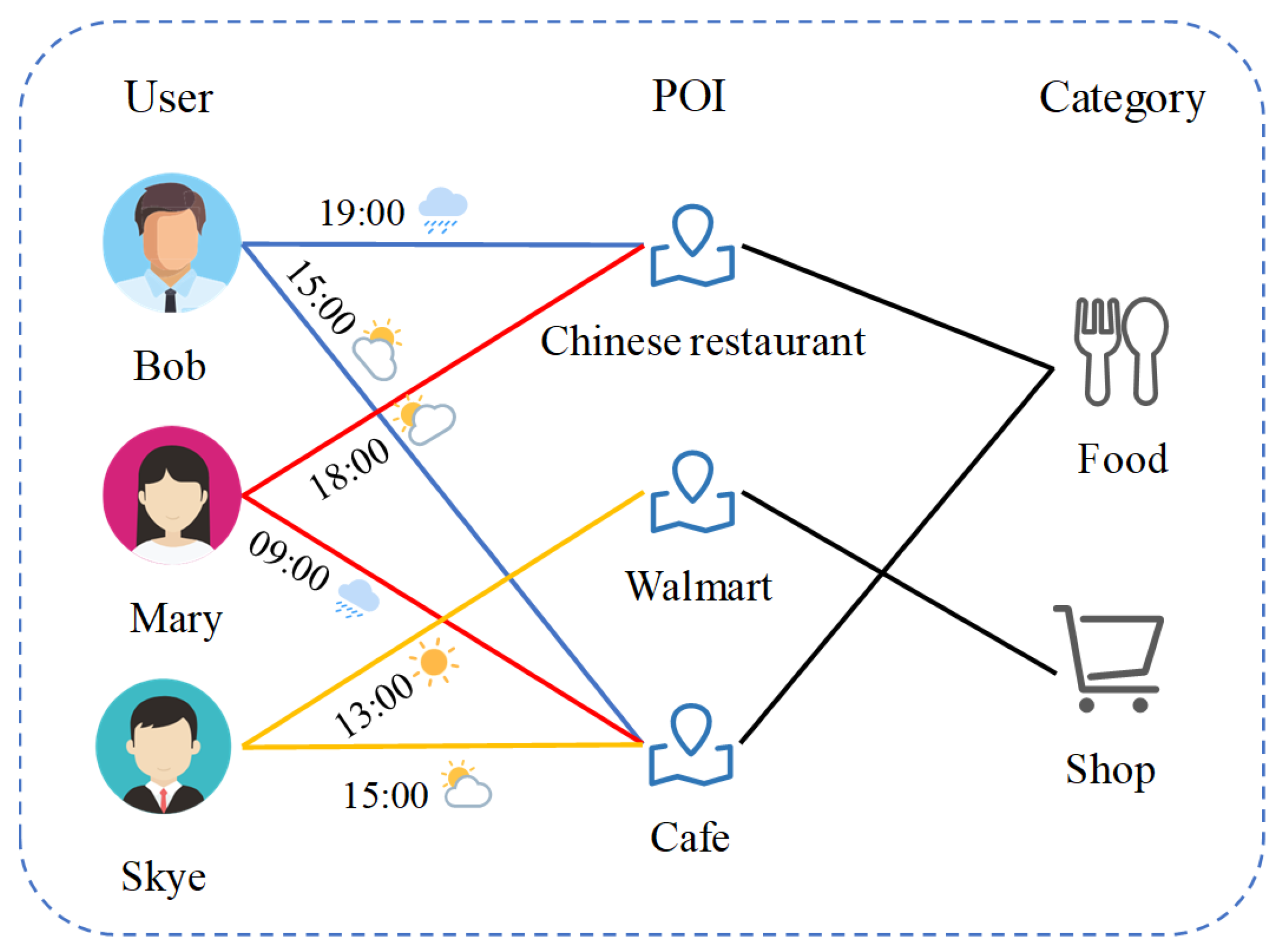
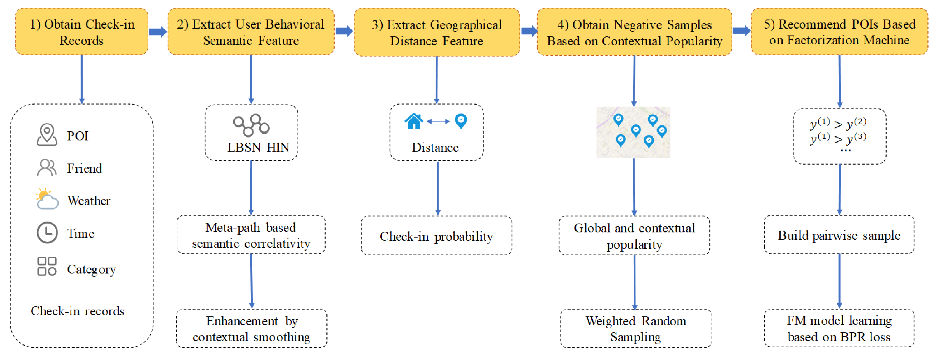
3. User Behavioral Semantic Feature Based on Check-in Contexts

This section elaborates how to extract users’ check-in features while considering the contextual information based on meta-path in LBSN Heterogeneous Information Network (HIN).

3.1. Semantic Correlativity Based on Meta-Path

As an abstract representation of the real world, the information network focuses on the connection between the different types of objects. When there exists more than one type of objects or one type of relations between objects, the network is called a Heterogeneous Information Network [22], or HIN. Thus, the complex relationships in LBSN can be represented through HIN as shown in Figure 1.
In order to mine fine-gained user behavioral semantic characteristics, the meta-path model, proposed in [23], is applied. For instance, a user is indirectly connected with a POI via a path U f r i e n d w i t h U c h e c k i n P , abbreviated as U U P , which means the user prefers the location checked in by thir friend. Moreover, the path U c h e c k i n P c h e c k i n b y U c h e c k i n P indicates that users prefer locations where people with common check-in records have checked in, which is a user-based collaborative recommendation. In this way, the recommendation can be made more explainable by designing such reasonable meta-paths to represent different user behavior semantics. Table 1 lists the meta-paths and their corresponding semantics, where G represents the category of POI.
Given the above definition of meta-path, the correlativity between users and POIs can be computed. The number of path instances between user u U and P O I p P through meta-path M is defined as P C M ( u , p ) , which reflects the relation strength directly. Then, the semantic correlativity between u and p can be defined as follows:
S C M ( u , p ) = P C M ( u , p ) P C M ( u , · )
where P C M ( u , · ) represents the total number of path instances starting from u through M. The user’s preference can be inferred from the location objects along the meta-path. On the other hand, the location objects adversely affect the user’s behavior preference. In other words, both the meta-path and its reverse one provide non-negligible semantic information. Thereout, the bidirectional semantic correlativity is defined as Equation (2) indicates. Here, M 1 represents the reverse meta-path of M:
B S C M ( u , p ) = S C M ( u , p ) + S C M 1 ( p , u ) 2 .
Let r u , p , c R represent the number of times that the user u U checks into the location p P at the context slot c C , such as r u , p , c = R ( B o b , C a f e , A f t e r n o o n ) . The bidirectional semantic correlativity for each element r u , p , c R can be computed as Equation (3) to obtain a new semantic tensor R M .
r ^ u , p , c = R M ( u , p , c ) = B S C M ( c ) ( u , p )
where B S C M ( c ) ( u , p ) is bidirectional semantic correlativity at context slot c.
After designing L meta-paths, the bidirectional semantic correlativity for tensor R through each meta-path can be then computed, and L semantic tensors R M 1 , R M 2 , , R M L are finally obtained.

3.2. Enhancement by Contextual Smoothing

The tensor R that incorporates the context information is obviously more sparse than the user-POI check-in matrix. Although R M , calculated for the proposed semantic correlativity, contains more non-zero elements than the original tensor R, the sparse problem still exists. To solve this problem, the mutual influence between context slots is considered to further mitigate the data sparseness by contextual smoothing.
It is believed that in LBSN, user behaviors at different context slots have a certain correlation. Taking the time context as an example, assuming that the user u visited the location p between 9 a.m. and 10 a.m., it is very likely that the user will also check in the location p between 10 a.m. and 11 a.m. Since these two time slots are all working hours, the user’s check-in behavior during these two time slots will be similar.
A new user behavior tensor B is constructed as Equation (4), where b u , p , c B indicates whether the user u has checked in the POI p at the context c:
b u , p , c = B ( u , p , c ) = 1 r u , p , c > 0 0 r u , p , c = 0 r u , p , c R .
Suppose b u , c = { b u , 1 , c , b u , 2 , c , , b u , P , c } as a check-in vector of user u at context c. For any two context slots c i and c j , the cosine similarity of user u’s check-in vector at the corresponding context slot is shown in Equation (5):
s i m u ( c i , c j ) = b u , c i b u , c j b u , c i 2 b u , c j 2 .
The similarity between the context slots c i and c j is the average of the similarities of all users, as shown in Equation (6):
s i m ( c i , c j ) = u U s i m u ( c i , c j ) | U | .
As shown in Figure 2, the 24 h of a day and the temperature (weather) range are divided into 8 slots, and the similarity of the three context slots with other slots analyzed, where the similarity between the same contexts slot is 1. As seen from the figure, the similarity between closer context slots is higher. Therefore, the semantic tensor R M can be smoothed based on the user behavior similarity between different context slots by giving higher weights on its neighboring slots:
r ˜ u , p , c = R ˜ M ( u , p , c ) = c C s i m ( c , c ) c C s i m ( c , c ) r ^ u , p , c .
Thus, with the contextual smoothing, the sparsity problem of original tensor R can be significantly alleviated.

4. The Distances and Check-In Probabilities

This section mainly explores the influence of the distance between the user’s home location and the POI they have checked in. Since the user does not generally indicate their home location, the latitude and longitude of the earth is first discretized into a certain number of 4.9 km × 4.9 km cells based on GeoHash [24], and then the average latitude and longitude of the cell with the most user check-in records are approximately set as the user’s home. It is generally agreed that the check-in probability decreases significantly as the distance to POI increases, and it follows the power-law distribution approximately [9]. The user’s geographical preference is indicated by the check-in probability of the user from their home (denoted as h u ) to x ( k m ) away location p, as shown in Equation (8):
y = P r ( h u , p ) = a · x b .
Let a = 2 w 0 and b = w 1 , and then Equation (8) is transformed into Equation (9) by taking the logarithm:
l o g y = w 0 + w 1 log x .
Let y = log y and x = log x , the linear regression method is employed to optimize the following loss function to obtain the regression coefficient:
L = 1 2 n = 1 N ( y p n ) 2 + λ 2 w 2
where w 0 and w 1 are regression coefficients, denoted by w , p n is real check-in probability to the x , and the regularization parameter λ is used to prevent the model from overfitting. Then the check-in probability is normalized by Equation (11):
P r u , p G = P r ( h u , p ) M a x ( P r u )
where the denominator represents the maximum check-in probability among the user u’s check-in records.

5. Recommendation Model

The Factorization Machine (FM) [25] was proposed to solve the feature combination problem under large-scale sparse data. For the context-specific recommendation scenario, user check-in data is segmented by context information such that the data is further sparse. Moreover, the user’s behavioral features may affect each other, so the Factorization Machine is very suitable for the target scenario of this paper. For the implicit feedback scenario of LBSN, a weighted random sampling strategy is proposed based on the popularity of POIs, and Bayesian Personalized Ranking [26] is employed to train the Factorization Machine model. The process of the recommendation model proposed in this paper is shown in Figure 3.

5.1. Weighted Random Sampling Based on Contextual Popularity

For the context-specific recommendation, it is necessary to first estimate the user’s preference for POIs at a certain context, and then recommend the Top-K unvisited POIs to the user according to preference. The training samples of the Factorization Machine consist of a large number of < u , p , c > triples, and each requires the features for model training. To do this, firstly, One-Hot [27] encoding is performed on users, POIs, and contexts to identify the specific sample. Secondly, assuming there are L meta-paths, L user behavior semantic tensors can be obtained, denoted as { R ˜ M 1 , R ˜ M 2 , , R ˜ M L } . Thus, each training sample will produce L semantic features, denoted as { r ˜ u , p , c 1 , r ˜ u , p , c 2 , , r ˜ u , p , c L } . Finally, the geographical distance feature constructed in Section 4 is added to complete the feature construction for each sample.
The record that the user actually has the check-in behavior can be regarded as a positive sample. However, the user does not indicate the location they do not like, meaning there are no negative samples. Therefore, a weighted random sampling method is proposed, which considers the context popularity to generate the negative samples needed for model training. If user u checked in POI p without visiting the locations around p, indicating that the user has a higher preference for p rather than the locations around it. In addition, the more times a POI in a region was checked in, the more popular it was, and the more likely it was to be known by users. On the other hand, if a user never checked in a very popular POI around the POI they checked in, it can be concluded that there is high probability they dislike to visit the former popular POI. For a given POI p, its popularity at context slot c is defined as follows.
P o p c ( p ) = ( 1 α ) | C K p | p P | C K p | + α | C K p , c | p P | C K p , c |
where | C K p | indicates the number of check-ins at p by all users and | C K p , c | indicates the number of check-ins at p at context slot c. In other words, the popularity of the POI p at context slot c is determined by its global popularity and contextual popularity. Here, α is the adjustive parameter.
For a sample < u , p , c > , a set of POIs within the range of k km around p is obtained, and the popularity P o p c ( p i ) is calculated as the sampling weight for each p i , to generate a weighted POIs set V = { p 1 , p 2 , , p i } . Here, a negative sampling method [28] is introduced, which involves the following two steps: (1) For each POI p i V , select a uniformly distributed random number u p i = r a n d ( 0 , 1 ) , and calculate the sampling score s p i = u p i ( 1 / P o p c ( p i ) ) and (2) select m POIs with the largest sampling score s p i as result samples.
Figure 4 presents an example of the extracted samples and features, where each row indicates a sample. The sample feature vector x ¯ ( i ) = ( x 1 , x 2 , , x | U | + | P | + | C | + L + 1 ) consists of five parts. The first part is the user’s One-Hot encoded binary vector, the length of which is the total number of users ( | U | ) . Similar to the first part, the second and third parts are binary vectors whose length is the total number of POIs ( | P | ) and the total number of context slots ( | C | ) respectively. The fourth part is the user behavioral semantic features of length L, where each dimension represents the feature value in the user behavioral semantic tensor extracted by a certain meta-path. The fifth part is the distance-based check-in probability introduced in Section 4. The target y ( i ) = y ^ ( x ¯ ( i ) ) represents the predicted value of the feature vector x ¯ ( i ) , i.e., the predicted preference of a certain user on a certain POI, in the Factorization Machine. As an illustrative example, Figure 4 gives two positive samples, i.e., < u 1 , p 1 , c 1 > and < u 2 , p 2 , c 2 > with their corresponding feature vectors x ¯ ( 1 ) and x ¯ ( 4 ) . For < u 1 , p 1 , c 1 > , it has two negative samples, < u 1 , p 2 , c 1 > and < u 1 , p 3 , c 1 > with their feature vectors x ¯ ( 2 ) and x ¯ ( 3 ) , which are framed in Figure 4. Similarly, < u 2 , p 2 , c 2 > has two negative samples, < u 2 , p 1 , c 2 > and < u 2 , p 3 , c 2 > with their feature vectors x ¯ ( 5 ) and x ¯ ( 6 ) .

5.2. Model Learning Based on Bayesian Personalized Ranking
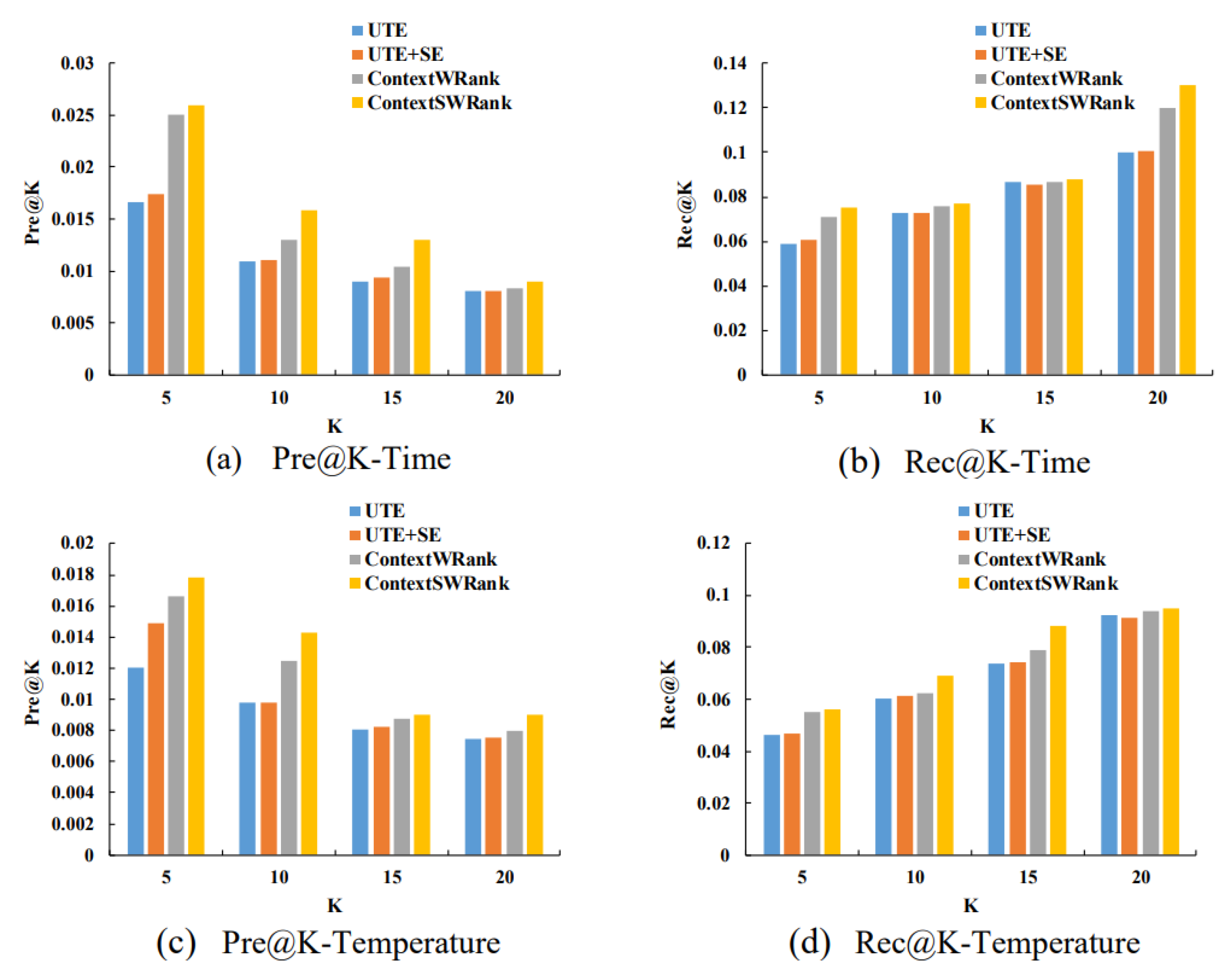
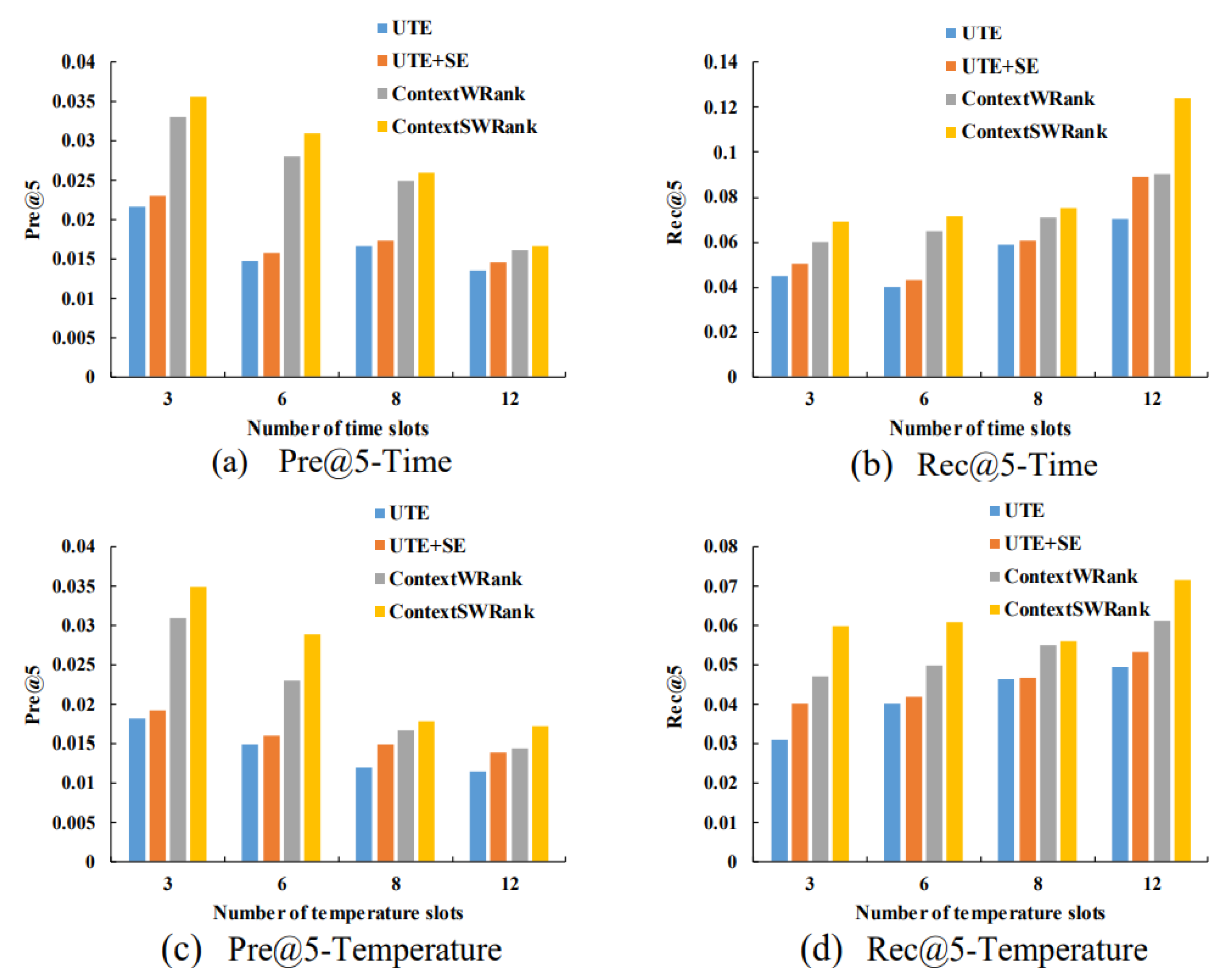
The expression of the Factorization Machine used in this paper is shown as Equation (13).
y ^ ( x ¯ ) = w 0 + i = 1 n w i x i + i = 1 n j = i + 1 n < v ¯ i , v ¯ j > x i x j
where n represents the number of features, w 0 is the global bias, and w i models the strength of the corresponding feature, v ¯ i = ( v i , 1 , v i , 2 , , v i , f ) is the f-dimensional latent factor vector of the i-th feature, and < v i , v j > represents the inner product of the two latent factor vectors. In addition, the quadratic term in Equation (13) intuitively introduces the combination of features in the model, which reflects the idea that the user behavior features interact with each other, and it is conducive to improving the recommendation performance.
LBSN often lacks negative feedback. In fact, the POIs where the user has not visited yet does not simply mean that they have no interest (they may not be able to find this location). Although the negative sampling is performed as in Section 5.1, it is unreasonable to directly treat the POIs where the user has not visited as negative samples to train the binary classification model. Therefore, a direct and effective recommendation model should be able to better rank the sample pairs for users, indicating that the user’s preference for the POIs the user has checked into is greater than the POIs the user has not checked into. Here, the idea of pair-wise learning is adopted. Taking the samples corresponding to u 1 as an example in Figure 4, it is converted into sample pairs in the form of y ( 1 ) > y ( 2 ) and y ( 1 ) > y ( 3 ) , which indicates that the user u 1 prefers the location p 1 instead of p 2 and p 3 . Consequently, the predicted value y ( 1 ) = y ^ ( x ¯ ( 1 ) ) obtained for p 1 is higher.
Based on the method proposed in [26], Equation (14) is used to express the probability that y ^ ( x ¯ ( i ) ) is larger than y ^ ( x ¯ ( j ) ) :
p ( i > u j | θ ) = 1 1 + e ( y ^ ( x ¯ ( i ) ) y ^ ( x ¯ ( j ) ) )
where θ represents the parameters used in the model, and > u represents the ordering relationship of two samples.
According to the Bayesian formula, if all samples need to be sorted correctly, it is required to maximize the following posterior probability:
p ( θ | > u ) p ( > u | θ ) p ( θ ) .
Assuming that the user’s ranking preference for sample pairs is independent, the likelihood function can be defined by:
p ( S | θ ) = u U p ( S u | θ ) = u U ( i > u j ) S u p ( i > u j | θ )
where S represents a set of ordering relationships of the sample pairs.
It is assumed that p ( θ ) is a Gaussian distribution [29] with zero mean and variance-covariance matrix θ = λ θ I . Thus, the objective function of ranking optimization can be formulated as:
O ( θ ) = ln p ( θ | > u ) = ln p ( > u | θ ) p ( θ ) = u U ( i > u j ) S u ln p ( i > u j | θ ) λ θ θ 2
where λ θ is a regularization parameter. Finally, Stochastic Gradient Descent (SGD) [30] is employed to optimize the above objective function:
O θ = u U ( i > u j ) S u ( θ ln p ( i > u j | θ ) θ λ θ θ 2 ) u U ( i > u j ) S u e ( y ^ ( x ¯ ( i ) ) y ^ ( x ¯ ( j ) ) ) 1 + e ( y ^ ( x ¯ ( i ) ) y ^ ( x ¯ ( j ) ) ) θ ( y ^ ( x ¯ ( i ) ) y ^ ( x ¯ ( j ) ) ) λ θ θ .
The gradient of each parameter is expressed in the form of Equation (19):
y ^ ( x ¯ ) θ = 1 i f θ i s w 0 x i i f θ i s w i x i j = 1 n v i , f x j v i , f x i 2 i f θ i s v i , f .
Afterwards, θ is updated along the negative gradient direction, which iterates over a certain number of times until the results converge or the iteration ends. After the model training is completed, the predicted value of user u for all POIs at context c can be calculated by Equation (13). Finally, the top K POIs that the user has not visited with the highest predicted value are recommended to the user.

6. Experiments

Experimental Datasets. The experiments were based on the Foursquare dataset (https://dropbox.com/s/pa1mni3h8qdkdby/Foursquare.zip?dl=0, accessed on 7 April 2019) provided by the author of literature [9], including real-world check-in data from 2010 to 2011. Each check-in record includes a user ID, a location ID, and a timestamp, where each location has its latitude, longitude and category information, and each user has their friends information. In addition, the APIs of darksky.net (https://darksky.net/dev, accessed on 24 April 2019) were used to collect the temperatures for each < l a t i t u d e , l o n g i t u d e , t i m e s t a m p > . Those locations which were visited by less than 10 users, and those users who visited less than 5 locations or had less than 10 check-ins, were removed. The statistics obtained after filtering the data are shown in Table 2.
In order to make the experiments more consistent with real situation, the training data D t r a i n and testing data D t e s t are split as follows: For each individual user, (1) aggregating user check-ins for each location; (2) sorting the location according to the first time that the user checked in; and (3) selecting the earliest 80% to train the model ( D t r a i n ) and using the remaining 20% to test the model ( D t e s t ).
Parameters Settings. The meta-paths listed in Table 1 are used to extract the user behavioral semantic features. The data were split according to the given number of context slots. For weather context, the temperature ranging from the minimum 4 °C to maximum 43 °C in the dataset were divided into 3, 6, 8, and 12 slots. For time context, the 24 h a day were also split into 3, 6, 8, and 12 slots. The parameters of check-in probability are obtained through learning, while others are summarized in Table 3. The software, libraries, packages used to code the model are python 2.7, numpy 1.16.5, py-geohash-any 1.1, scipy 1.2.1, sklearn 0.20.3, pandas 0.24.2, and fastFM 0.2.11.
Evaluation Metrics. Two widely-used metrics are used to evaluate the performance of different recommendation methods, namely precision and recall, denoted by Pre@K and Rec@K, where K is the number of recommended POIs. Given a user u and context c, t p u , c is the number of POIs contained in both the ground truth and Top-K results, f p u , c is the number of POIs in the Top-K results but not in the ground truth, and t n u , c is the number of POIs contained in ground truth but not in the Top-K results. Pre@K(c) and Rec@K(c) for context slot c are computed as follows [12]:
P r e @ K ( c ) = u U t p u , c u U ( t p u , c + f p u , c )
R e c @ K ( c ) = u U t p u , c u U ( t p u , c + t n u , c ) .
The overall precision and recall are calculated by averaging the precision and recall over all context slots.
P r e @ K = 1 | C | c C P r e @ K ( c )
R e c @ K = 1 | C | c C R e c @ K ( c ) .
Comparison Methods. The followings are used as the comparison methods:
  • UTE [12]: A collaborative recommendation model which incorporates temporal influence for time-specific POI recommendation;
  • UTE+SE [12]: A collaborative recommendation model which incorporates both temporal and geographical influence for time-specific POI recommendation;
  • ContextWRank: The proposed model in this paper, but does not employ contextual smoothing method given in Section 3.2;
  • ContextSWRank: The proposed model in this paper, which employ contextual smoothing method in Section 3.2.
Performance Comparison. As shown in Figure 5, the precision and recall of different methods is compared, considering the time and weather (temperature) contexts when the context slot is set to 8. As it reveals, UTE+SE exhibits better results than UTE in most cases, which demonstrates the effectiveness of considering geographical influence. Meanwhile, ContextWRank outperforms UTE and UTE+SE, in terms of Pre@5 at time comparison, by 50.3% and 44% respectively. Furthermore, with the enhancement of contextual smoothing, ContextSWRank shows the best performance in all cases.
Effect of the Number of Context Slots.Figure 6 compares the precision and recall with the different numbers of context slots from 3 to 12 when considering time and weather (temperature) contexts. Obviously, the smaller number of slots, the less context-specific it is. As Figure 6 indicates, when the number of context slots is set to 3 or 6, Pre@5 achieves the best and Rec@5 achieves the worst for all methods. When the number of context slots increases, Pre@5 drops whereas Rec@5 increases in general. Finally, Pre@5 reaches the worst and Rec@5 reaches the best at 12 context slots for all methods. The reason may be that the more slots, the sparser the data will be, which leads to the recommendation become more difficult. On the other hand, the increasing number of slots makes the number of ground truth of POIs become fewer for each slot, thus leading to the better recall. Most importantly, ContextWRank and ContextSWRank always achieve the better performance than UTE and UTE+SE no matter how many context slots there are, which further proves the effectiveness of the proposed method.
Spatial Visualization of POI recommendation.Figure 7 demonstrates the visited, recommended and visited, and recommended but not visited POIs for Bob, Mary, and Skye, as an example. It could be obviously found that the recommended POIs are reasonable if considering their homes and contexts.

7. Threats to Validity

The model provided in this paper gives the context-specific Point-of-Interest recommendation based on popularity-weighted random sampling and Factorization Machine. However, its validities may still be limited. In the following, we discuss the threats to its internal and external validities.
Threats to internal validity concern factors that could have influenced the results. In the study, this is mainly due to the contextual factors that influence the model performance. ContextSWRank considers the most important factors: Time, distance, and temperature. It is worth investigating some other factors like social relationships. However, most datasets lack such information. Another threat to internal validity is its applicability. In fact, ContextSWRank consumes more computing and memory resources than some other baselines because it involves many contextual information. However, ContextSWRank has shown its satisfactory capability when dealing with the test data.
Threats to external validity concern the generalization of the results. Here, one particular concern comes from the dataset for the evaluation. It could be argued that the performance could vary with different datasets. However, it is difficult to obtain such real check-in records which contains rich contextual information. Although the dataset holds the check-in records dating several years ago, many recent researchers have evaluated their models on such traditional real-world datasets, as indicated in [10,31]. In addition, because Foursquare is a very popular LBSN, the public available dataset from Foursquare provides a solid environment for effective testing. In the future, the proposed model could be further evaluated on other datasets if possible.

8. Conclusions and Future Work

Nowadays, many people like to share the places they visit in Location-based Social Networks (LBSNs). Point of Interest (POI) recommendation, as one of location-based services, helps users find new locations to visit. Previous studies have made great success on POI recommendation by employing geographical influence and user preference. However, we believe that the human decision on where to visit is very complex and involves contextual factors. This paper proposed a context-specific POI recommendation model called ContextSWRank. Specially, a bidirectional influence correlativity metric between users and POIs was proposed to measure the user behavioral semantic feature, and a contextual smoothing method was introduced to effectively alleviate the data sparsity. In addition, the check-in probability was computed based on the geographical distance between the user’s home and the POI. Furthermore, to handle the problem of none negative feedback in LBSN, a weighted random sampling method based on contextual popularity was proposed. Finally, the recommendation results were obtained by incorporating multiple features in Factorization Machine with Bayesian Personalized Ranking loss. The experimental results on a real dataset collected from Foursquare demonstrated that the proposed approach achieved the better recommendation performance than other methods. In the future, the following issues need to be further studied: (a) Deeply explore the influence factors on user behavior in LBSN; (b) improve the user experience by speeding up the recommendation process; and (c) test the model on other popular datasets to further evaluate its effectiveness.

Author Contributions

Dongjin Yu and Kaihui Xu jointly designed and developed the architecture and conceptual model of the proposed recommendation model. Yi Shen implemented and investigated experimental results. Dongjin Yu and Kaihui Xu conceived the main idea presented in this manuscript. Yi Shen contributed to the architecture design and reviewed experimental results. Kaihui Xu, Yihang Xu, and Yi Shen wrote the manuscript. All authors provided critical feedback and helped shape the research, analysis, and manuscript. All authors have read and agreed to the published version of the manuscript.

Funding

This work was partially supported by National Natural Science Foundation of China (No. 61472112, No. 61702144), and Key Science and Technology Project of Zhejiang Province of China (No. 2017C01010).

Institutional Review Board Statement

Not applicable.

Informed Consent Statement

Not applicable.

Data Availability Statement

Publicly available datasets were analyzed in this study. This data can be found here: [https://dropbox.com/s/pa1mni3h8qdkdby/Foursquare.zip?dl=0 (accessed on 7 April 2019)].

Acknowledgments

The authors would like to acknowledge anonymous reviewers who gave the valuable comments to improve the quality of the manuscript.

Conflicts of Interest

The authors declare no conflict of interest.

References

  1. Gao, H.; Tang, J.; Hu, X.; Liu, H. Exploring temporal effects for location recommendation on location-based social networks. In Proceedings of the Seventh ACM Conference on Recommender Systems, Hong Kong, China, 12–16 October 2013; pp. 93–100. [Google Scholar] [CrossRef]
  2. Trattner, C.; Oberegger, A.; Eberhard, L.; Parra, D.; Marinho, L.B. Understanding the Impact of Weather for POI Recommendations. In CEUR Workshop Proceedings, Proceedings of the Workshop on Recommenders in Tourism Co-Located with 10th ACM Conference on Recommender Systems (RecSys 2016), Boston, MA, USA, 15 September 2016; CEUR-WS.org; Fesenmaier, D.R., Kuflik, T., Neidhardt, J., Eds.; ACM: New York, NY, USA, 2016; Volume 1685, pp. 16–23. [Google Scholar]
  3. Ye, M.; Yin, P.; Lee, W.; Lee, D.L. Exploiting geographical influence for collaborative point-of-interest recommendation. In SIGIR 2011, Proceeding of the 34th International ACM SIGIR Conference on Research and Development in Information Retrieval, Beijing, China, 25–29 July 2011; Ma, W., Nie, J., Baeza-Yates, R., Chua, T., Croft, W.B., Eds.; ACM: New York, NY, USA, 2011; pp. 325–334. [Google Scholar] [CrossRef]
  4. Lian, D.; Zhao, C.; Xie, X.; Sun, G.; Chen, E.; Rui, Y. GeoMF: Joint geographical modeling and matrix factorization for point-of-interest recommendation. In KDD’14, Proceeding of the 20th ACM SIGKDD International Conference on Knowledge Discovery and Data Mining, New York, NY, USA, 24– 27 August 2014; Macskassy, S.A., Perlich, C., Leskovec, J., Wang, W., Ghani, R., Eds.; ACM: New York, NY, USA, 2014; pp. 831–840. [Google Scholar] [CrossRef]
  5. Liu, Y.; Pham, T.; Cong, G.; Yuan, Q. An Experimental Evaluation of Point-of-interest Recommendation in Location-based Social Networks. Proc. VLDB Endow. 2017, 10, 1010–1021. [Google Scholar] [CrossRef]
  6. Bao, J.; Zheng, Y.; Wilkie, D.; Mokbel, M.F. Recommendations in location-based social networks: A survey. GeoInformatica 2015, 19, 525–565. [Google Scholar] [CrossRef]
  7. Kulkarni, S.; Rodd, S.F. Context Aware Recommendation Systems: A review of the state of the art techniques. Comput. Sci. Rev. 2020, 37, 100255. [Google Scholar] [CrossRef]
  8. Ye, M.; Yin, P.; Lee, W. Location recommendation for location-based social networks. In Proceedings of the 18th ACM SIGSPATIAL International Symposium on Advances in Geographic Information Systems, San Jose, CA, USA, 3–5 November 2010; pp. 458–461. [Google Scholar] [CrossRef]
  9. Li, H.; Ge, Y.; Hong, R.; Zhu, H. Point-of-Interest Recommendations: Learning Potential Check-ins from Friends. In Proceedings of the 22nd ACM SIGKDD International Conference on Knowledge Discovery and Data Mining, San Francisco, CA, USA, 13–17 August 2016; pp. 975–984. [Google Scholar] [CrossRef]
  10. Cai, L.; Wen, W.; Wu, B.; Yang, X. A coarse-to-fine user preferences prediction method for point-of-interest recommendation. Neurocomputing 2021, 422, 1–11. [Google Scholar] [CrossRef]
  11. Aliannejadi, M.; Rafailidis, D.; Crestani, F. A Joint Two-Phase Time-Sensitive Regularized Collaborative Ranking Model for Point of Interest Recommendation. IEEE Trans. Knowl. Data Eng. 2020, 32, 1050–1063. [Google Scholar] [CrossRef] [Green Version]
  12. Yuan, Q.; Cong, G.; Ma, Z.; Sun, A.; Magnenat-Thalmann, N. Time-aware point-of-interest recommendation. In Proceedings of the 36th International ACM SIGIR Conference on Research and Development in Information Retrieval, Dublin, Ireland, 28 July–1 August 2013; pp. 363–372. [Google Scholar] [CrossRef]
  13. Yuan, Q.; Cong, G.; Sun, A. Graph-based Point-of-interest Recommendation with Geographical and Temporal Influences. In Proceedings of the 23rd ACM International Conference on Conference on Information and Knowledge Management, Shanghai, China, 3–7 November 2014; pp. 659–668. [Google Scholar] [CrossRef]
  14. Si, Y.; Zhang, F.; Liu, W. An adaptive point-of-interest recommendation method for location-based social networks based on user activity and spatial features. Knowl. Based Syst. 2019, 163, 267–282. [Google Scholar] [CrossRef]
  15. Zhao, H.; Yao, Q.; Li, J.; Song, Y.; Lee, D.L. Meta-Graph Based Recommendation Fusion over Heterogeneous Information Networks. In Proceedings of the 23rd ACM SIGKDD International Conference on Knowledge Discovery and Data Mining, Halifax, NS, Canada, 13–17 August 2017; pp. 635–644. [Google Scholar] [CrossRef]
  16. Wang, Z.; Juang, J.; Teng, W. Predicting POI visits with a heterogeneous information network. In Proceedings of the Conference on Technologies and Applications of Artificial Intelligence, TAAI 2015, Tainan, Taiwan, 20–22 November 2015; pp. 388–395. [Google Scholar] [CrossRef]
  17. Unger, M.; Bar, A.; Shapira, B.; Rokach, L. Towards latent context-aware recommendation systems. Knowl. Based Syst. 2016, 104, 165–178. [Google Scholar] [CrossRef]
  18. Chang, B.; Jang, G.; Kim, S.; Kang, J. Learning Graph-Based Geographical Latent Representation for Point-of-Interest Recommendation. In Proceedings of the 29th ACM International Conference on Information and Knowledge Management, Virtual Event, Ireland, 19–23 October 2020; pp. 135–144. [Google Scholar] [CrossRef]
  19. Ma, Y.; Gan, M. Exploring multiple spatio-temporal information for point-of-interest recommendation. Soft Comput. 2020, 24, 18733–18747. [Google Scholar] [CrossRef]
  20. Yu, F.; Cui, L.; Guo, W.; Lu, X.; Li, Q.; Lu, H. A Category-Aware Deep Model for Successive POI Recommendation on Sparse Check-in Data. In Proceedings of the Web Conference 2020, Taipei, Taiwan, 20–24 April 2020; pp. 1264–1274. [Google Scholar] [CrossRef]
  21. Kang, W.; McAuley, J. Self-Attentive Sequential Recommendation. In Proceedings of the 2018 IEEE International Conference on Data Mining (ICDM), Singapore, 17–20 November 2018; pp. 197–206. [Google Scholar] [CrossRef] [Green Version]
  22. Shi, C.; Li, Y.; Zhang, J.; Sun, Y.; Yu, P.S. A survey of heterogeneous information network analysis. IEEE Trans. Knowl. Data Eng. 2017, 29, 17–37. [Google Scholar] [CrossRef]
  23. Sun, Y.; Han, J.; Yan, X.; Yu, P.S.; Wu, T. PathSim: Meta Path-Based Top-K Similarity Search in Heterogeneous Information Networks. Proc. VLDB Endow. 2011, 4, 992–1003. [Google Scholar] [CrossRef]
  24. Morton, G.M. A Computer Oriented Geodetic Data Base and a New Technique in File Sequencing; Technical Report; IBM Ltd.: Ottawa, ON, Canada, 1966. [Google Scholar]
  25. Rendle, S. Factorization Machines. In Proceedings of the 10th IEEE International Conference on Data Mining, Sydney, Australia, 14–17 December 2010; pp. 995–1000. [Google Scholar] [CrossRef] [Green Version]
  26. Rendle, S.; Freudenthaler, C.; Gantner, Z.; Schmidt-Thieme, L. BPR: Bayesian Personalized Ranking from Implicit Feedback. In Proceedings of the Twenty-Fifth Conference on Uncertainty in Artificial Intelligence, Montreal, QC, Canada, 18–21 June 2009; pp. 452–461. [Google Scholar]
  27. Harris, D.; Harris, S. Digital Design and Computer Architecture, 2nd ed.; Morgan Kaufmann: Waltham, MA, USA, 2012; p. 129. [Google Scholar]
  28. Efraimidis, P.S.; Spirakis, P.G. Weighted Random Sampling. In Encyclopedia of Algorithms—2008 Edition; Kao, M., Ed.; Springer: Berlin, Germany, 2008; pp. 1024–1027. [Google Scholar] [CrossRef]
  29. Lukacs, E. A Characterization of the Normal Distribution. Ann. Math. Stat. 1942, 13, 91–93. [Google Scholar] [CrossRef]
  30. Bottou, L. Stochastic Gradient Descent Tricks. In Neural Networks: Tricks of the Trade, 2nd ed.; Montavon, G., Orr, G.B., Müller, K.R., Eds.; Springer: Berlin, Germany, 2012; pp. 421–436. [Google Scholar] [CrossRef] [Green Version]
  31. Su, Y.; Zhang, J.D.; Li, X.; Zha, D.; Xiang, J.; Tang, W.; Gao, N. FGRec: A Fine-Grained Point-of-Interest Recommendation Framework by Capturing Intrinsic Influences. In Proceedings of the 2020 International Joint Conference on Neural Networks (IJCNN), Glasgow, UK, 19–24 July 2020; pp. 1–9. [Google Scholar] [CrossRef]
Figure 1. An example of Location-Based Social Network (LBSN) Heterogeneous Information Network (HIN) of user-Point-Of-Interest (POI)-category with contexts of time and weather.
Ijgi 10 00258 g001
Figure 2. User behavior similarity between different context slots.
Ijgi 10 00258 g002
Figure 3. The context-specific POI recommendation process.
Ijgi 10 00258 g003
Figure 4. An example for representing a context-specific POI recommendation problem with feature vectors.
Ijgi 10 00258 g004
Figure 5. Performance comparisons of different methods considering time and weather contexts.
Ijgi 10 00258 g005
Figure 6. Performance comparisons with different numbers of context slots.
Ijgi 10 00258 g006
Figure 7. Spatial visualization of POI recommendation.
Ijgi 10 00258 g007
Table 1. Meta-paths and their semantics.
SymbolMeta-PathSemantics
M 1 U P Users prefer locations they have
checked in
M 2 U U P Users prefer locations where their
friends have checked in
M 3 U P U P Users prefer locations where people
with common check-in records have checked in
M 4 U P G P Users prefer the same category of locations
they have checked in
M 5 U P G P U P Users prefer locations where people have same
category of check-in records have checked in
Table 2. Statistics of dataset.
# Users# POIS# Categories# Check_ins# Social LinksSparsity
27928414127234,04914,93299.61%
Table 3. Parameter settings.
ParameterValues
the number of context slots3, 6, 8, 12
the adjustive parameter α 0.4
the number of latent factors f6
regularization parameters λ 0.01
the range of distance k when sampling2
the number of negative samples m5
Publisher’s Note: MDPI stays neutral with regard to jurisdictional claims in published maps and institutional affiliations.

