
G-STC-M Spatio-Temporal Analysis Method for Archaeological Sites


1
School of Resources and Environment, Anhui Agricultural University, Hefei 230036, China
2
Key Laboratory of Virtual Geographic Environment, Nanjing Normal University, Ministry of Education, Nanjing 210023, China
*
Author to whom correspondence should be addressed.
ISPRS Int. J. Geo-Inf. 2021, 10(5), 312; https://0-doi-org.brum.beds.ac.uk/10.3390/ijgi10050312
Submission received: 2 March 2021
/
Revised: 1 May 2021
/
Accepted: 2 May 2021
/
Published: 7 May 2021
Abstract
:Based on the significant hotspots analysis method (Getis-Ord Gi* significance statistics), space-time cube model (STC) and the Mann–Kendall trend test method, this paper proposes a G-STC-M spatio-temporal analysis method based on Archaeological Sites. This method can integrate spatio-temporal data variable analysis and the space-time cube model to explore the spatio-temporal distribution of Archaeological Sites. The G-STC-M method was used to conduct time slice analysis on the data of Archaeological Sites in the study area, and the spatio-temporal variation characteristics of Archaeological Sites in East China from the Tang Dynasty to the Qing Dynasty were discussed. The distribution of Archaeological Sites has temporal hotspots and spatial hotspots. Temporally, the distribution of Archaeological Sites showed a gradual increasing trend, and the number of Archaeological Sites reached the maximum in the Qing Dynasty. Spatially, the hotspots of Archaeological Sites are mainly distributed in Jiangsu (30°~33° N, 118°~121° E) and Anhui (29°~31° N, 117°~119° E) and the central region of Zhejiang (28°~31° N, 118°~121° E). Temporally and spatially, the distribution of Archaeological Sites is mainly centered in Shanghai (30°~32° N, 121°~122° E), spreading to the southern region.
1. Introduction
In archaeology, “Archaeological Sites” refers to the remains of ancient human activities, which exist in the process of historical development with important value [1,2,3]. By analyzing Archaeological Sites and understanding the characteristics of their spatio-temporal variation, it is helpful to deepen the understanding of Archaeological Sites in historical periods.
According to the archaeological records and historical materials summarized by scholars in the past, we can see that in the Tang Dynasty, the hotspots of human activities were mainly distributed in Yangzhou Prefecture, Changzhou Prefecture and Hangzhou Prefecture. In Song Dynasty, Hangzhou Prefecture, Taizhou Prefecture and Luzhou Prefecture became hotspots of human activities. In the Yuan Dynasty, Ningguo Prefecture appeared in hotspots. In Ming Dynasty, hotspots were mainly distributed in Suzhou Prefecture, Anqing Prefecture and Ningguo Prefecture. In the Qing Dynasty, Fengyang Prefecture and Yingzhou Prefecture also became the main hotspots of human activities [4,5,6]. These archaeological records are mainly recorded by the original data of physical materials in the form of words and images [7,8,9]. There are some comparisons of historical data, but the volume of data is incomplete, and the extent of the regions divided by each dynasty is not consistent, which affects the analysis of the archaeological record.
Archaeological Sites include ancient cultural sites, ancient tombs, ancient buildings, grotto carvings and other categories (such as ancient wells, ancient roads, etc.). They are characterized by incomplete residual, with a certain geographical scope [10,11]. At present, the main methods of spatio-temporal analysis and expression of Archaeological Sites are as follows: statistical index analysis method of spatial data, representation of spatio-temporal model and analysis method of spatial statistics changing with time. The statistical index analysis method of spatial data is based on the statistical indicators of the centralized trend in statistics, combined with the descriptive analysis method of events, and puts forward the statistical indicators to describe the centralized trend in spatial analysis. This method mainly includes the data local spatial autocorrelation analysis method [12,13,14] and the data and time series-related hierarchical analysis method [15]. The purpose of the data local spatial autocorrelation analysis method is to determine whether the variables are spatially correlated and how relevant they are. It contains cluster analysis [16,17], factor analysis [18], correspondence analysis [19], regression analysis [20,21] and hotspots analysis [22,23]. Among them, the hotspots analysis method refers to the Getis-Ord Gi* statistical calculation method for each element in the Archaeological Sites dataset. Using the data calculated by this method, we can clearly judge the clustering location of high- or low-value elements in space. This method can better test the data of Archaeological Sites and identify whether there are statistically significant hotspots of Archaeological Sites among the research objects. The data and time series-related hierarchical analysis method is a statistical method for dynamic data processing, which studies the statistical rule of random data and time series correlation. It mainly includes stationary time series analysis [24], the ensemble empirical mode decomposition method [25,26] and Mann–Kendall trend test analysis [27,28]. Among them, Mann–Kendall trend test analysis is a statistical method to test the correlation between the value of Archaeological Sites and the rank of time series in the study of Archaeological Sites. The advantage of Mann–Kendall trend test analysis is that it is not required to follow a certain distribution of research samples and is not disturbed by a small number of outliers. This method is more suitable for type variables and sequence variables, and the calculation is relatively simple.
The spatio-temporal model is a kind of geographic model which can effectively organize and manage temporal geographic data. It has more complete attribute, spatio-temporal semantics, and expresses the dynamic structure changing with time [29]. The spatio-temporal model is mainly used in the analysis of temporal changes of geospatial data. Usually, it contains an event-based spatio-temporal data model [30], spatio-temporal object model [31], base state with amendments model [32], sequent snapshots model [33], space-time composite model [34] and space-time cube model [35,36,37]. Among them, the space-time cube model combines two-dimensional spatio-temporal dimension, and displays the change characteristics of spatio-temporal data from three-dimensional space in the form of a cube. This form can better combine the spatial location and age data of Archaeological Sites, and more intuitively and clearly express the spatio-temporal distribution of Archaeological Sites.
The analysis method of spatial statistics changing with time is also a method used to study the spatio-temporal distribution of Archaeological Sites. This method includes spatial statistical index time series analysis and spatio-temporal index change analysis. The spatial statistical index time series analysis reflects the change of spatial pattern with time. The commonly used methods include composition analysis [38], comparative analysis of the same kind [39], multi-index analysis [40] and temporal trend analysis [41]. Among them, temporal trend analysis can analyze the spatial statistical value of Archaeological Sites according to the corresponding time series, so as to obtain the variation trend of the spatial statistics of Archaeological Sites and time. This method is practical and widely used, which clearly expresses the spatial differentiation characteristics of Archaeological Sites [42]. In addition, the change of spatial statistics with time can also be shown by spatio-temporal index change analysis. The spatio-temporal change is regarded as the change of spatial distribution with time, and the spatial statistics are made at each time point respectively, and then linked together according to the time sequence to reflect the change of spatial statistical index. The spatio-temporal index change analysis method is usually realized by spatio-temporal slice analysis. Spatio-temporal slice analysis refers to the method of time segmentation of a group of long time series data of Archaeological Sites, and then statistical spatial distribution of each time series, and finally, comparative analysis of spatial statistics of different time series sites. The spatio-temporal slice analysis method makes it easier to process the spatio-temporal data with a large amount of information and analyzes the spatial distribution changes of Archaeological Sites with different time series in a more detailed way, which provides a strong support for accurately describing the spatial differentiation characteristics and evolution process of Archaeological Sites.
This paper proposes a method to study the spatio-temporal distribution of Archaeological Sites, which combines the analysis of spatial statistical index, the space-time cube model and the analysis of temporal variation of spatial statistics. In this method, (1) the statistical index analysis of spatial data is used to judge the spatio-temporal correlation of Archaeological Sites’ data, (2) the space-time cube model is used to express the spatio-temporal distribution of Archaeological Sites and (3) spatio-temporal variation analysis of spatial statistics is used to explore the spatio-temporal variation of Archaeological Sites in the study area. Finally, this method is used to analyze the time-slice data of Archaeological Sites, and the spatio-temporal variation characteristics of Archaeological Sites are obtained.
The research results are helpful to deepen the understanding of the spatio-temporal distribution of Archaeological Sites in historical periods, and also promote the interpretation of the law of human activities and facilitate the further development of the excavation and protection of Archaeological Sites [43,44,45].
2. Research Area and Research Method
2.1. Archaeological Data
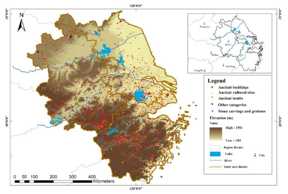
The area studied in this paper is located in east China (27°02′–35°20′ N,114°54′–123°10′ E), including Anhui province, Zhejiang province, Jiangsu province and Shanghai city, with a total area of about 359,140 km2. These areas are dominated by hills, basins and plains, with an obvious monsoon climate, densely covered rivers and lakes and rich historical and cultural resources.
According to China’s State Administration of cultural heritage listed among the first to eighth batch of provincial-level cultural relics protection unit information guide, this paper selects the study area in the Tang Dynasty, Song Dynasty, Yuan Dynasty, Ming Dynasty and the Qing Dynasty, five dynasties in the Archaeological Sites in the national and provincial cultural relics protection unit, as the research object (a total of 1846 sites). The published information includes the geographical location of the Archaeological Sites, the dynasty in which it existed and the type of archaeological site it belongs to. In terms of the dynasties to which the Archaeological Sites belong, the Archaeological Sites of Tang, Song, Yuan, Ming and Qing dynasties are respectively 67, 191, 57, 623 and 908. In terms of the type of Archaeological Sites, ancient cultural sites, ancient buildings, ancient tombs, stone carvings and grottoes and other categories are respectively 109, 1463, 134, 112 and 30, as shown in Table 1.
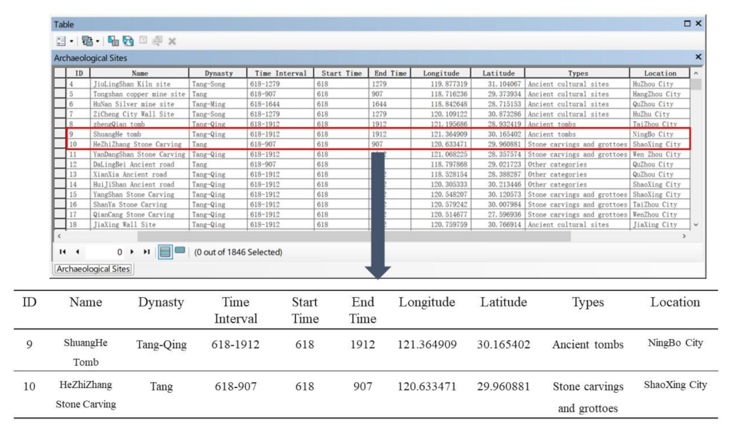
We collected the spatial longitude and latitude of these Archaeological Sites’ data and input all the attribute values into the analysis tool to get the database of the research object. In the Archaeological Sites database, each Archaeological Site is represented by the corresponding point data. Its attribute values include ID, name, dynasty, time interval, start time, end time, longitude, latitude, types and the corresponding geographic location, as shown in Figure 1.
2.2. Getis-Ord Gi* Statistical Method of Significant Cold- and Hot-Spots
Getis-Ord Gi* is a statistical method proposed by Getis and Ord in 1995 for identifying hotspots in spatial datasets [46,47]. Local spatial autocorrelation between Archaeological Sites describes the correlation between Archaeological Sites in the study area and its neighboring provinces (municipalities directly under the Central Government). As an indicator for evaluating local spatial autocorrelation, local Getis-Ord Gi* statistics are used to determine whether the Archaeological Sites in the study area are clustered with high values (hotspots) or low values (cold spots). In this paper, the Getis-Ord Gi* method was used to identify the cold- and hot-spots with statistical significance among the Archaeological Sites within the study area. Local statistics of Getis-Ord Gi* can be expressed as (Equation (1)):
where: xi is the attribute value of Archaeological Sites element j, and w(i,j) is the space weight between the Archaeological Sites elements i and j. When the element j falls in the neighborhood space range and time range of the target element i at the same time, w(i,j) = 1; otherwise, w(i,j) = 0, and n is the total number of elements. Equations (2) and (3) are as follows:
In the equations, Gi* statistics return a Z-score, which is a multiple of standard deviation and reflects the dispersion degree of a dataset.
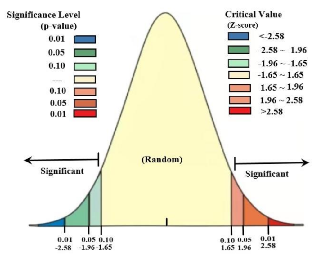
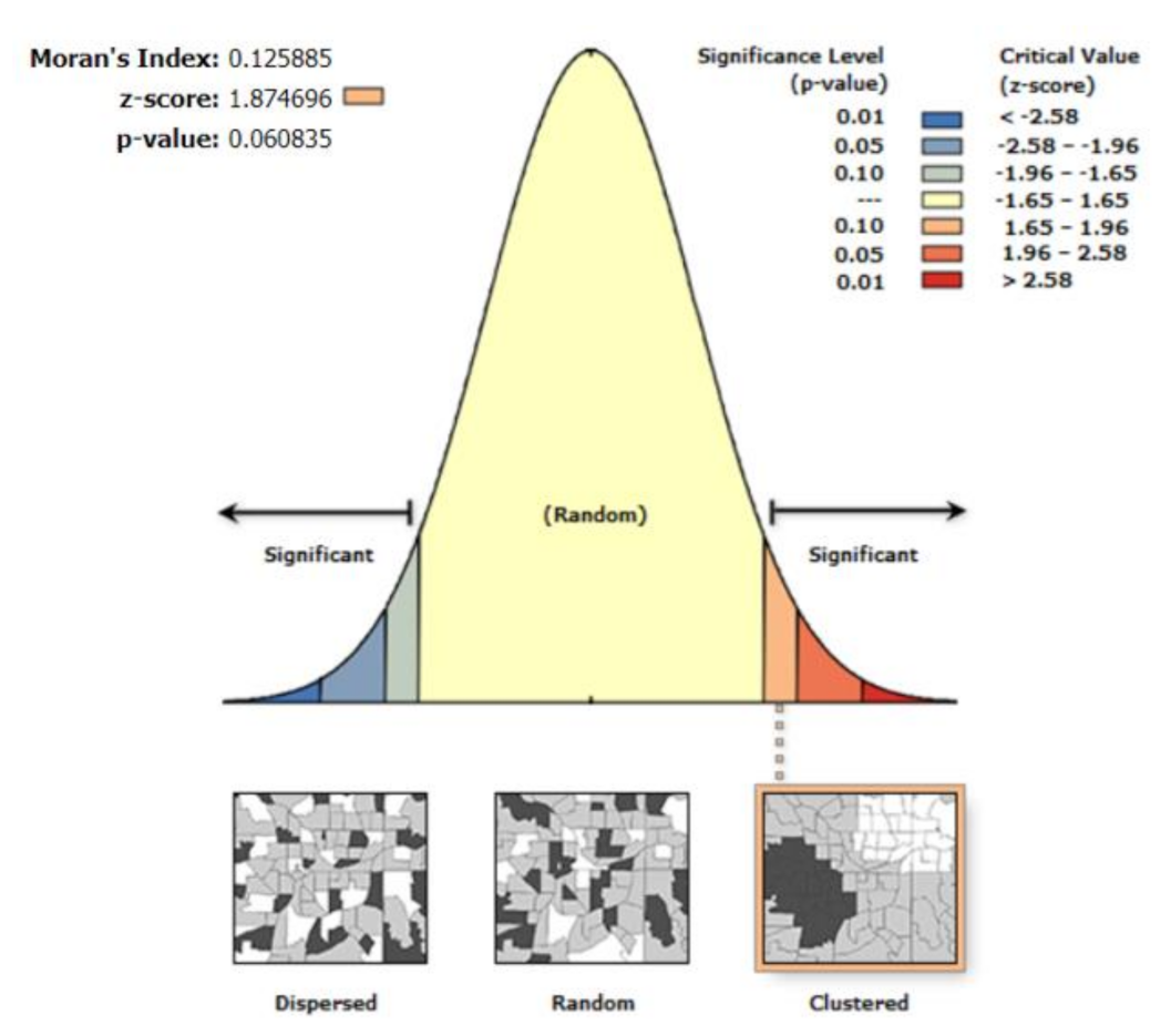
The prerequisite for using Getis-Ord Gi* to calculate the significant cold- and hot-spots of Archaeological Sites is that the Archaeological Sites’ datasets have spatial clustering characteristics. Based on the null hypothesis of the random distribution of Archaeological Sites, this paper first carries out element model analysis. Element model analysis is mainly used to judge the spatial correlation of Archaeological Sites. The Z-score and p-value calculated by this analysis tool can be used to determine whether the Archaeological Sites’ data shows statistically significant clustering characteristics or discrete patterns. In a normal distribution, Z-scores and p-values are used to measure the spatial distribution pattern. Z-score is a multiple of standard deviation, reflecting the dispersion degree of a dataset. The p-value represents the probability, and reflects the probability of an event [48]. As shown in Figure 4, if on both ends of the statistical results appear very high or very low Z-scores, corresponding to the smaller p-values, the Archaeological Sites are detected with a point spatial distribution pattern of a dataset that does not conform to the null hypothesis represented by a random pattern, whereas if the absolute value of Z-score is higher, corresponding to the larger p-values, it represents that the Archaeological Sites of point data have obvious characteristics of spatial clustering.
The spatial distribution of Archaeological Sites’ data is tested by “confidence”. Confidence refers to the proportion of data with spatial clustering characteristics in the data of Archaeological Sites. Confidence is a necessary prerequisite for rejecting the null hypothesis. In general, confidence is 90%, 95% or 99%, among which 99% represents rejection of the null hypothesis, that is, the spatial position in a certain region does not present a completely random distribution.
If the data of Archaeological Sites show spatial clustering characteristics through element pattern analysis, then Getis-Ord Gi* is used to calculate the significant cold- and hot-spots of Archaeological Sites. However, using the Getis-Ord Gi* method can only calculate the cold- and hot-spots of Archaeological Sites in space, which shows the distribution of high-value clustering or low-value clustering of Archaeological Sites in space. The time attribute of Archaeological Sites is not fully utilized.
2.3. Construction of Space-Time Cube Model
The spatio-temporal scale includes the time scale and space scale. In this paper, we use the Knox method for spatio-temporal scale calculation. Determining a spatio-temporal scale is the premise of expressing the space-time cube. If the scale is too large, the accuracy of space-time cube analysis may be affected; if the scale is too small, a large number of empty columns may appear [49,50]. In spatial clustering analysis, the Knox spatio-temporal interaction test method is usually used to find the variation rules of spatial distribution of data in different spatial scopes, and according to the obtained variation rules, it can be used as a reference to determine the distance threshold in clustering analysis [51]. In this paper, the Knox spatio-temporal interaction test method is used to explore the aggregation patterns of Archaeological Sites under different time and space conditions, and on this basis, the spatio-temporal scale of the space-time cube of Archaeological Sites is calculated.
In this paper, it is assumed that there are n Archaeological Sites in space-time, and the Knox method first combines all Archaeological Sites in pairs to form N Archaeological Sites point pairs, as shown in Equation (4). Meanwhile, a critical value is defined on both time (t) and space (d). Then, the adjacency relationship between the Archaeological Site pairs is judged one by one. If the spatial distance of two Archaeological Sites is between [0, d], then these two Archaeological Sites belong to spatial proximity. The number of adjacent Archaeological Sites is counted, and Ns is defined as the logarithm of adjacent Archaeological Sites in space. If the time interval between two Archaeological Sites is between [0, t], then these two Archaeological Sites belong to the time adjacent, and Nt is defined as the log of the time-adjacent Archaeological Sites. Only when two Archaeological Sites both meet spatio-temporal adjacency can the pair of Archaeological Sites be judged as spatio-temporal adjacency. According to the adjacent relationship between the two Archaeological Sites, the observed value, K, is the statistical test quantity, as shown in Equation (5):
where m and n respectively represent Archaeological Site m and Archaeological Site n in the Archaeological Sites pair. Dmn represents the spatial adjacency relationship between the Archaeological Site pairs. If the Archaeological Sites m and n are adjacent in space, Dmn = 1; otherwise, Dmn = 0. Tmn is the temporal adjacency relationship between the Archaeological Site pairs. If the Archaeological Sites m and n are adjacent in time, Tmn = 1; otherwise, Tmn = 0.
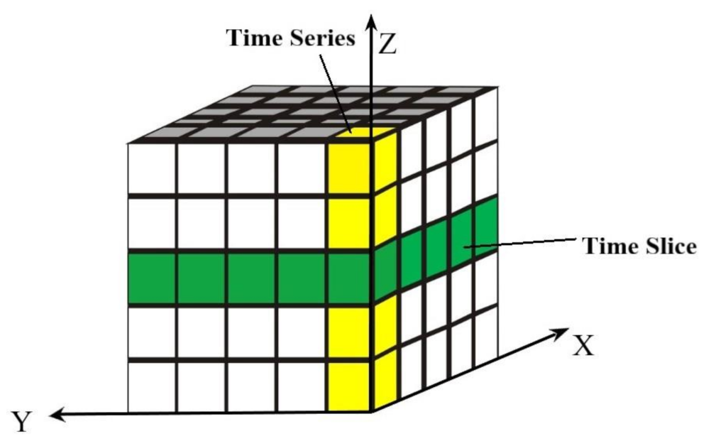
We use the space-time cube to express the space-time dimension. The space-time cube model was proposed by Hagerstrand, who introduced the time axis into the traditional two-dimensional space and expressed spatio-temporal data by constructing the space-time cube [52]. Each space-time cube is made up of a single space-time bar, consisting of rows, columns and time steps. In the space-time cube, the number of rows multiplied by the number of columns multiplied by the number of time steps is the total number of columns in the space-time cube. The rows and columns of the space-time cube describe the spatial position of geographical objects, and the time step of the space-time cube represents the time attribute of the geographical object. The space-time cube is constructed to intuitively show the spatial characteristics and attribute characteristics of geographical entities (or phenomena) changing with time in the three-dimensional space, as shown in Figure 5.
In this paper, Archaeological Sites’ points are aggregated into spatio-temporal columns, in which rows and columns describe the geographical location of Archaeological Sites’ points, and time steps describe the historical time of Archaeological Sites’ points. The space-time cube of the Archaeological Sites is visualized through a number of spatio-temporal columns, in which each column represents the change of the Archaeological Sites at a certain location over time, and the total column represents the change of the Archaeological Sites at different locations at different times. The columns covering the same location and distributed in different time step ranges share the same location and constitute a column time series in the Archaeological Sites dataset. Columns covering the same time range and distributed at different spatial locations share the same time and constitute a time slice in the Archaeological Sites dataset. The space-time cube model of the Archaeological Sites can be seen as a three-dimensional cube composed of a large number of spatio-temporal columns at different spatial positions.
The advantage of creating the space-time cube model of Archaeological Sites is that it is very intuitive to express the temporal attributes of Archaeological Sites. If the integration of mathematical statistical methods is lacking, the spatial and temporal distribution of Archaeological Sites cannot be quantitatively described. On the other hand, as the amount of data increases, the manipulation of the cube becomes more and more complex, to the point that it eventually becomes unmanageable.
2.4. Mann–Kendall Trend Test Method
The Mann–Kendall method, proposed by Mann and Kendall, is a test method for correlation analysis between the numerical value of statistical geographical phenomena and the rank of time series [53]. The test method of Mann–Kendall is non-parametric (no distribution test). Its advantage is that the test premise does not require the samples of Archaeological Sites to follow a certain distribution law or be disturbed by a few outliers, and it can accurately test the changes of the data variables of Archaeological Sites that increase or decrease over time.
In this paper, the Mann–Kendall test is used to test the variation trend of the space-time cube distribution in Archaeological Sites. At each location with data, the Mann–Kendall trend method performs tests on the time series of spatio-temporal columns of independent Archaeological Sites. The trend of the time series of each space-time bar will be recorded as a Z-score and a p-value. A small p-value indicates that the trend has statistical significance. Symbols associated with a Z-score can determine whether the trend is an increase in spatio-temporal bars (positive Z-score) or a decrease in space-time bars (negative Z-score). For the time series, X = {x1, x2, …, xn,}, and the Mann–Kendall trend test is as shown in Equations (6) and (7):
When n is greater than or equal to 10, the spatio-temporal column statistic, S, of the Archaeological Sites basically obeys a normal distribution, with a mean value of 0, and the variance is calculated as in Equations (8) and (9):
The Mann–Kendall method can be used to detect the changing trend of Archaeological Sites and the significance of the changing trend. However, this method can only be used for trend analysis of time series. If combined with the Archaeological Sites space-time cube, the space-time bar value trend of the geographical position of each Archaeological Site can be measured, and the time series trend of the Archaeological Sites in the whole study area can be obtained.
2.5. G-STC-M Method
The G-STC-M method refers to the research method of spatio-temporal distribution of Archaeological Sites, which integrates Getis-Ord Gi*, the space-time cube model and the Mann–Kendall trend test method. Getis-Ord Gi* is used to judge the spatio-temporal correlation of Archaeological Sites’ data, the space-time cube model is used to express the spatio-temporal distribution of Archaeological Sites and the Mann–Kendall trend test method is used to explore the spatio-temporal variation of Archaeological Sites in the study area.
In this method, the space-time cube model of the Archaeological Sites was first constructed, the standard space-time cube of the Archaeological Sites is only the expression of the number of Archaeological Sites in space-time, and then, the significant cold- and hot-spots were counted for each spatio-temporal column. The space-time cube calculated by the Getis-Ord Gi* statistical method can show the appearance of cold- and hot-spots of Archaeological Sites in space-time. Secondly, the Mann–Kendall trend statistical method was used to analyze the trend of the time series of each column of the space-time cube of the Archaeological Sites, with Z-value obtained by the Getis-Ord Gi* statistical method. In this method, all site data are integrated into a space-time cube model to display the spatio-temporal data in a three-dimensional state and reflect its spatio-temporal characteristics. Combined with G and M methods of spatio-temporal data variable analysis, the spatio-temporal hotspots and their variation trends of Archaeological Sites are quantitatively analyzed. Finally, by using this method and slicing analysis of the space-time cube, the spatio-temporal variation characteristics of Archaeological Sites are obtained.
The technical process is shown in Figure 6.
3. Experiment
In this experiment, ArcGIS® Pro of Esri Company was used as the experimental tool.
3.1. Calculation of Significant Cold- and Hot-Spots at Archaeological Sites
The cluster analysis tool in the ArcGIS® Pro spatial statistics tool was used to conduct element model analysis on the Archaeological Sites in the study area. The start time in the data attribute of Archaeological Sites was set as the analysis field to conduct spatial correlation analysis. The results show that the Z-score was 1.874696, and the p-value was 0.060835. In other words, the Archaeological Sites present spatial clustering characteristics, as shown in Figure 7. Then, the hotspot analysis tool was selected to calculate the significant cold- and hot-spots of Archaeological Sites. By classifying the calculated Gi* statistic (Gi_Bin), Z-score and p-value, the standard of cold and hot clustering degree can be obtained.
If Gi_Bin is zero and the Z-value is between −1.65 and 1.65, the corresponding p-value is greater than 0.1, which means that there are no statistically significant cold spots or hotspots in the study area. When the values of Gi_Bin appear as 1, 2 and 3, it indicates that hotspots exist in the distribution of sites in the study area. Furthermore, the larger the value of Gi_Bin, the higher the confidence degree, and the probability of Archaeological Sites’ hotspots clustering is greater, as shown in Table 2.
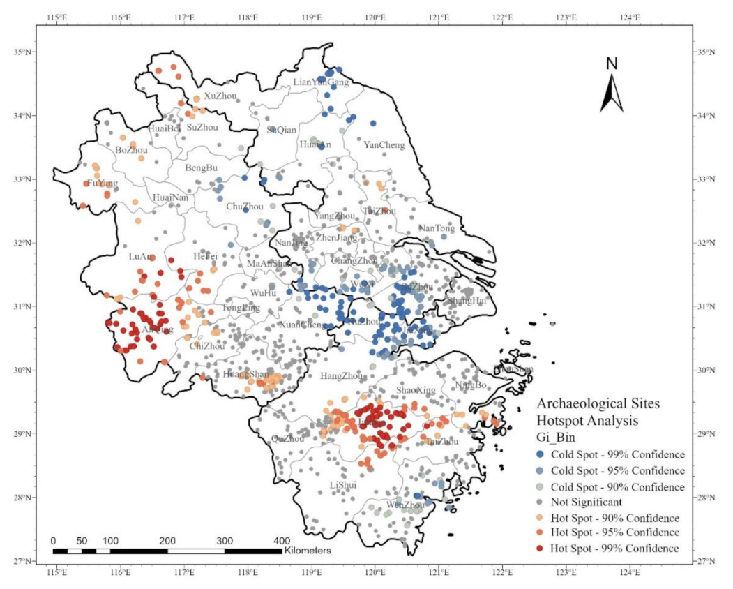
According to the degree of cold and hot clustering, the cold- and hot-spots’ distribution map of the Archaeological Sites is visualized. Finally, the spatial distribution diagram of the hotspots of Archaeological Sites was obtained, as shown in Figure 8.
The hotspots in the research area are mainly distributed in Anhui and Zhejiang provinces, while the cold spots are mainly distributed at the intersection of Anhui, Zhejiang and Jiangsu provinces: parts of northern Anhui (33°~35° N, 115°~117° E), such as Fuyang and Bozhou, and western Anhui (30°~32° N, 116°~117° E), such as Anqing, Lu’an and Hefei. In the central region of Zhejiang (28°~30° N, 119°~131° E), such as Jinhua, Taizhou and Ningbo, the positive Z-score and p-value obtained by Getis-Ord Gi* statistics are relatively high, corresponding confidence value is relatively high and the high-value clustering degree is relatively large, and these areas have become hotspots of spatio-temporal distribution of Archaeological Sites.
The corresponding cold spots are mainly distributed at the intersection of the three provinces (30°~32° N, 119°~121° E), such as Suzhou, Jiaxing, Huzhou, Xuancheng and Wuxi. In some regions, the Z-score shows a trend of gradual decrease. The negative Z-score is small, and the low-value clustering is close, making it a cold spot for spatio-temporal distribution of Archaeological Sites.
3.2. Constructing the Space-Time Cube Model of the Archaeological Sites
3.2.1. Space-Time Cube Scale Analysis of Archaeological Sites
Based on the sites of the five historical dynasties in the research area, in this paper, a series of space-time cubes with different time intervals and distance intervals were constructed. Based on these cubes, the spatio-temporal hotspots analysis was conducted, and the research results were compared. Then, the appropriate time and space analysis scales were determined by combining with Knox space–time interaction test method. This experiment was performed in the ArcGIS® Pro Space-Time Pattern Mining Tools, selecting the Create Space-Time Cube by Aggregating Points tool to create the space-time cube model of the Archaeological Sites, and selecting the Start Time in the Archaeological Sites data as the time field.
Under the condition of setting the same time interval, the distance between the space-time cubes in the Archaeological Sites is increased continuously to study the differences of spatial differentiation features of the cube models constructed under different distance intervals. The results show that with the increase of distance interval, the number of empty columns in the cube decreases obviously, the overall growth trend of the number of Archaeological Sites remains stable, the number of cold- and hot-spots in the same hotspots analysis spatio-temporal domain gradually decreases and the proportion of cold- and hot-spots in space and time decreases, as shown in Table 3.
Under the condition of setting the same distance interval, the time interval of the space-time cube of the Archaeological Sites is increased continuously, and the difference of the evolution process of the cube model constructed under different time intervals is studied. The results show that with the increase of distance interval, the number of empty columns in the cube decreases significantly, the overall growth trend of the number of Archaeological Sites remains stable, the number of cold and hotspots in the same hotspots analysis spatio-temporal range gradually decreases and the proportion of cold- and hot-spots in space-time decreases, as shown in Table 4.
Combined with the Knox spatio-temporal interaction test method, the space-time cube model of Archaeological Sites’ points was established at a time interval of 50 years and a space interval of 100 km.
3.2.2. The Space-Time Cube Expression of Archaeological Sites
The space-time cube of the Archaeological Sites’ data converges 1846 points into 340 mesh positions through 11 time-steps. Each location is 50 km by 50 km squared. The entire space-time cube of the Archaeological Sites’ data spans 850 km from west to east and 1000 km from north to south. The duration of each time step interval is 100 years, so the entire time period covered by the space-time cube of the Archaeological Sites’ data is 1100 years. Of the 340 total locations, 189 (55.59%) are effective locations, which contain at least one point. The 189 locations were composed of 2079 time-boxes, of which 479 (23.04%) had point counts greater than zero.
The symbolized cube directly expresses the spatio-temporal trend changes of the Archaeological Sites’ data. The darker the color of the column is, the more Archaeological Sites that appeared in that period. A single gray cube indicates that the number of Archaeological Sites is 1 or less than 1. According to the cube diagram, the spatio-temporal distribution of the Archaeological Sites and the changing trend of each time stage can be analyzed, showing the changes of Archaeological Sites from the Tang Dynasty to the Song Dynasty, as shown in Figure 9.
3.3. The Space-Time Cube Trend Analysis of Archaeological Sites
At each spatio-temporal column position of the Archaeological Sites’ space-time cube, the Mann–Kendall trend tested the independent spatio-temporal column time series. The values of the spatio-temporal bars of the first period are compared with the values of the spatio-temporal bars of the second period. If the former is less than the latter, the comparison result is given as 1. If the former is greater than the latter, the comparison result is −1. If the two are equal, the comparison result is 0. Sum the comparison results for each pair of time periods. If the expected sum is 0, then there is no trend in the spatio-temporal bar in the space-time cube over time. The trend of the time series of each spatio-temporal bar will be recorded as a Z-score and a p-value. Z-scores and p-values are both measures of statistical significance.
If the Z-value is high, it indicates that the sequence of changes in Archaeological Sites is in an upward trend. If the Z-value is close to 0, it indicates that there is no significant change trend, and the significance of the change trend is graded, as shown in Table 5.
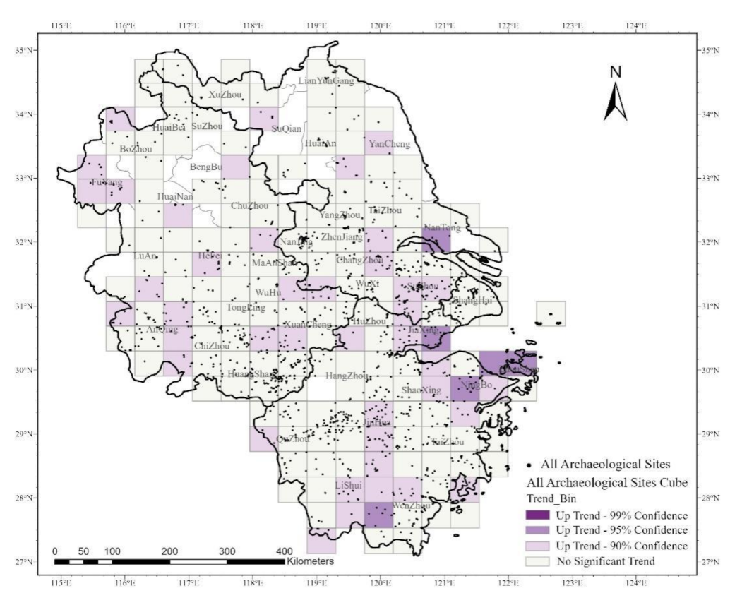
Based on the space-time cube model of Archaeological Sites’ data, the trend test of the whole space-time cube model of Archaeological Sites’ data and the time series of each column was carried out by using the Mann–Kendall trend test method. This experiment selected the Visualize Space Time Cube in 2D tool under Utilities and set the display theme to trends to conduct the space-time cube trend analysis of Archaeological Sites. The results are visualized hierarchically by the value of Trend_Bin, as shown in Figure 10.
As can be seen from the figure, the purple region is the time series of the Archaeological Sites’ data bars with an upward trend. Among 189 data cube locations of Archaeological Sites, 47 data cube locations of Archaeological Sites showed an upward trend. On the whole, these upward trending space-time cube bars are mainly distributed in the marginal areas and some central areas, and it shows that the distribution of Archaeological Sites in these areas is increasing in time and space. Among them, belonging to Anhui Province, there were 17 spatio-temporal columns, accounting for 29.79%. Belonging to Jiangsu Province, there were 9 spatio-temporal columns, accounting for 19.14%, and belonging to Zhejiang province, there were 21 spatio-temporal columns, accounting for 44.68%.
3.4. The G-STC-M Method for Archaeological Sites
In this paper, based on the space-time cube model of Archaeological Sites, Getis-Ord Gi* statistical method and Mann–Kendall trend test were combined to identify the spatio-temporal cold- and hot-spot trend changes of Archaeological Sites.
Firstly, the time slice of each Archaeological Sites’ data (TIME_STEP_ID) is taken as the unit to calculate the local Getis-Ord Gi* statistics values of all spatial positions on the time slice. Then, the Getis-Ord Gi* statistics Z-score and p-value of each Archaeological Sites’ data cube position are obtained. Finally, the distribution trend of the cold- and hot-spots in the spatial position in the time series is obtained. According to the Getis-Ord Gi* statistical analysis results of each column and the Mann–Kendall trend test results of each spatio-temporal column containing the Archaeological Sites’ data, the spatio-temporal variation rules of the cold- and hot-spots of each location were judged, and the recognized spatio-temporal cold- and hot-spots were classified. The cold- and hot-spots’ pattern classification is shown in Table 6.
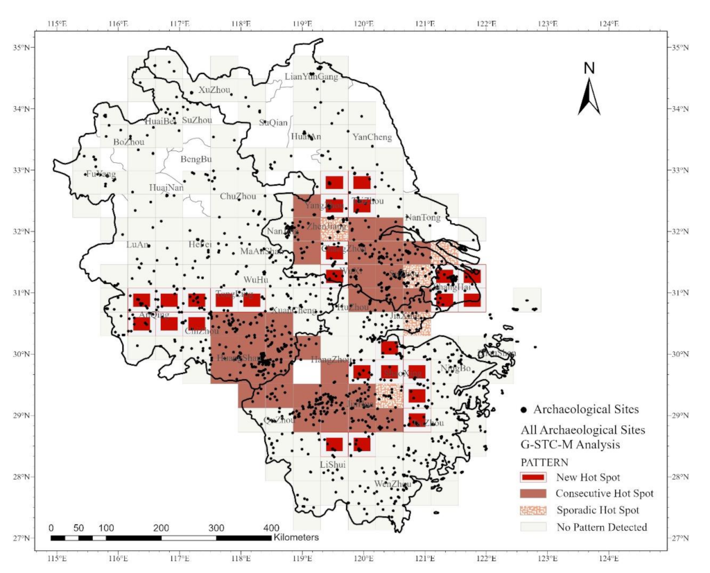
The spatio-temporal cold- and hot-spots trend analysis of Archaeological Sites is based on the space-time cube of the above Archaeological Sites’ points as input data. According to the space-time cube created, the spatio-temporal hotspots analysis is carried out, and the corresponding Z-score and p-value are obtained through statistical analysis of each column. This experiment selected the Visualize Space Time Cube in 2D tool under Utilities and set the display theme to hot- and cold-spot trends to conduct the spatio-temporal variation trends of Archaeological Sites. Then, according to the definition of the spatio-temporal trend pattern of cold- and hot-spots, the result diagram is obtained, as shown in Figure 11. By analyzing the spatio-temporal hotspots of the Archaeological Sites created by the space-time cube, the Archaeological Sites can be visually displayed on the map in the form of cold- and hot-spots to express their spatio-temporal variation trends.
It can be seen from the figure that among 189 data cubes of Archaeological Sites, 64 cube positions are hotspot distribution positions. Among them, there are 26 newly added hotspots, 33 consecutive hotspots and 5 dispersed hotspots.
The hotspots are mainly distributed in the southern part of Jiangsu and Anhui provinces, the central part of Zhejiang province and Shanghai region and the southern Part of Jiangsu province (30°~33° N, 119°~121° E), such as Taizhou, Changzhou and Suzhou. In the eastern part of Zhejiang (29°~31° N, 116°~119° E), such as Huzhou, Jiaxing, Hangzhou, Shaoxing, Quzhou, Jinhua and Lishui, these areas contain newly added hotspots, continuous hotspots and dispersed hotspots. Shanghai mainly has new hotspots, while the southern part of Anhui (30°~33° N, 119°~121° E), such as Xuancheng, Tongling, Anqing, Chizhou and Huangshan, contains new hotspots and continuous hotspots.
4. Analysis and Discussion
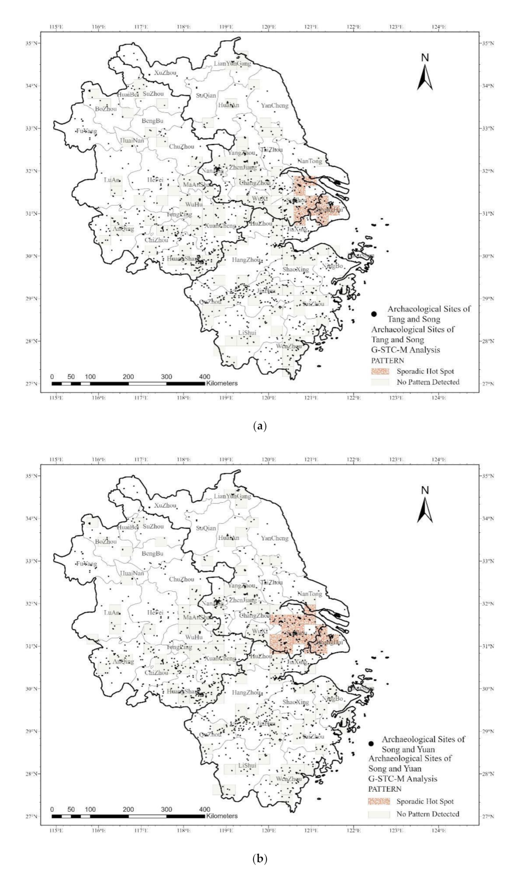
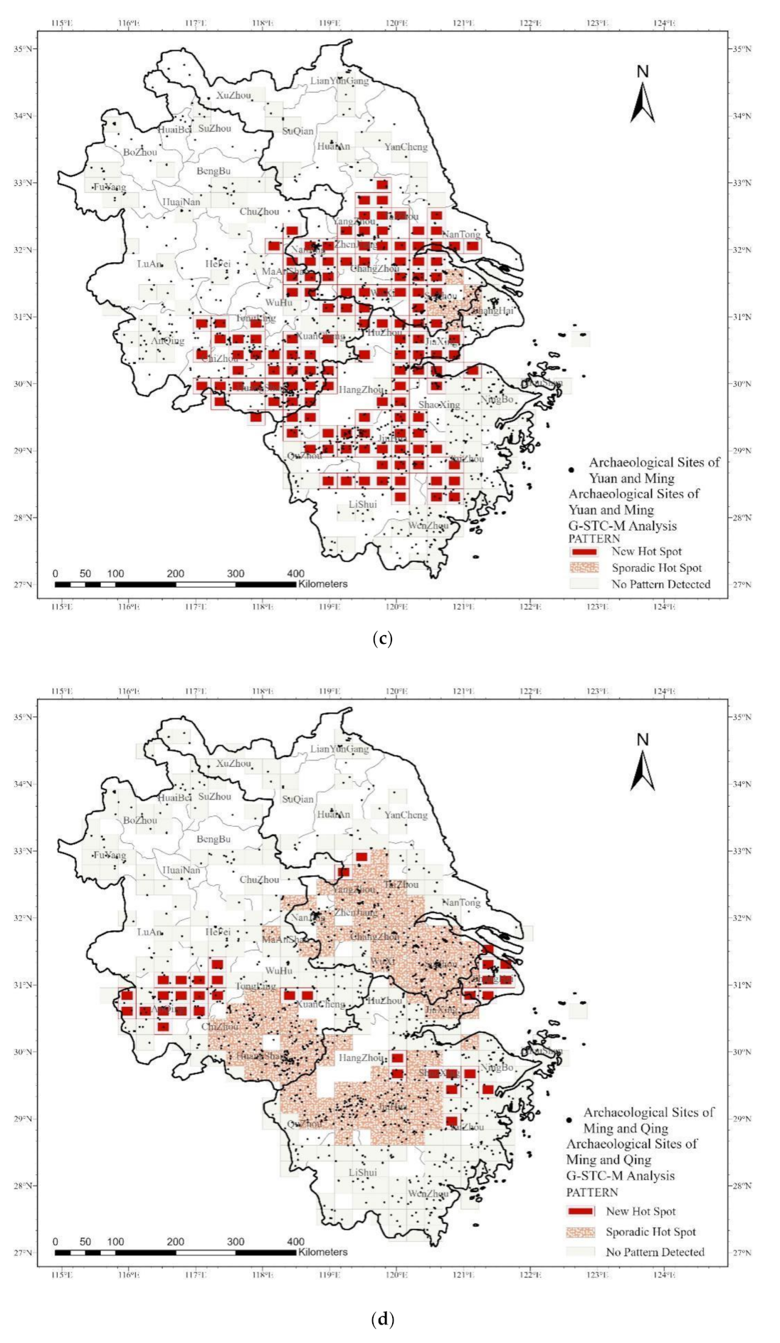
In order to better analyze the spatio-temporal changes of Archaeological Sites and reflect the changing state of ancient human activities, the time interval of the Archaeological Sites’ data is divided more carefully, that is, the Archaeological Sites’ data in the study area is analyzed by time slice based on the G-STC-M method. The data of the Archaeological Sites in the research area includes five dynasties in terms of time. After 1293, the time series data are divided into four adjacent time intervals (Tang–Song, Song–Yuan, Yuan–Ming and Ming–Qing), and the significant cold hotspots’ distribution of the space-time cube of the Archaeological Sites’ data in the adjacent dynasties is obtained, as shown in Figure 12 and Figure 13.
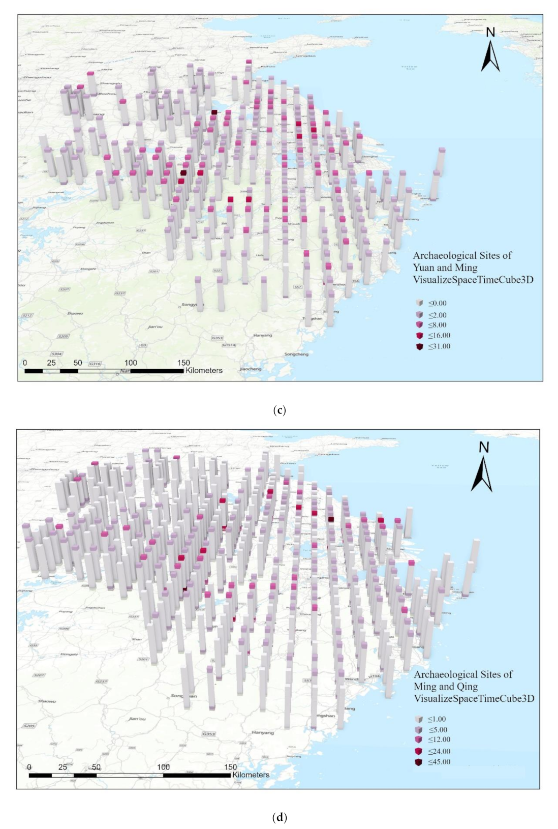
The number and location of hotspots in Archaeological Sites changed between different adjacent dynasties. From the Tang Dynasty to the Qing Dynasty, more and more dark cubes appeared, and the number of Archaeological Sites gradually increased, indicating that human activities gradually expanded. In addition, in the analysis based on the G-STC-M method, the number of newly added hotspots gradually increased from scattered hotspots to more and more new hotspots, and the number of newly added hotspots reached the maximum in Yuan and Ming Dynasties, and finally, the number of dispersed hotspots was the most obvious in Ming and Qing Dynasties.
In the Tang and Song Dynasties, only continuous hotspots appeared, mainly distributed in the southeast part of the study area (30°~32° N, 120°~122° E), such as Suzhou, Jiaxing and Shanghai. In the Song and Yuan Dynasties, the number of continuous hotspots increased, and the newly added hotspots were Changzhou, Huzhou and Nantong. In the Yuan and Ming Dynasties, new hotspots began to appear, mainly distributed in the south of Anhui province (29°~31° N, 117°~ 119° E), such as Chizhou, Tongling, Xuancheng, Huangshan, Wuhu and Maanshan, the southern part of Jiangsu province (30°~33° N, 118°~121° E), such as Changzhou, Nanjing, Zhenjiang, Yangzhou and Taizhou area, and the central part of Zhejiang province (28°~31° N, 118°~121° E), such as Hangzhou, Huzhou, Jiaxing, Jinhua, Shaoxing, Taizhou and Lishui area. The expanding range of new hotspots suggests that that human activity is shifting towards these areas and that they are beginning to converge. Finally, in the Ming and Qing Dynasties, most of the new hotspots in the Yuan and Ming Dynasties were transformed into continuous hotspots, and new hotspots also appeared, such as Anqing and Ningbo. The continuous hotspots were mainly distributed in the central part of the whole research area (29°~331° N, 117 °~ 121° E). Human activities in these areas were relatively concentrated.
In the past, the study of the state of ancient human activity change, using the observation and indirect inference of archaeological material, can only obtain the archaeological records, such as the natural language description of the text or the expression of the historical plane map. In this study, we used the method of space-time expression and mathematical statistics to analyze the time slice of ancient sites and used the integrated expression of time-space to show the spatial-temporal distribution of Archaeological Sites, quantify the trend of the spatial-temporal distribution of cold- and hot-spots and determine the corresponding spatial location of the cold- and hot-spots, so as to show the change state of human activities. This enriches the method of studying the temporal and spatial distribution of Archaeological Sites in space archaeology on the basis of previous studies [54,55].
However, in the use of mathematical statistics, the accuracy of research results is closely related to the accuracy of research data [56]. According to the archaeological records, the accuracy of the time attribute data of Archaeological Sites needs to be improved. In the future, with the closer connection between archaeology and other sciences, the research field of archaeology will be more extensive, and the content of research will be more in-depth [57,58,59]. Archaeological methods will not only be combined with mathematical statistics, but also with artificial intelligence technology [60]. Archaeological research content and research methods will continue to enrich, and archaeological records will continue to increase.
5. Conclusions
In this paper, a research method of spatio-temporal variation law based on the G-STC-M method for spatio-temporal analysis of Archaeological Sites was proposed. In the analysis of spatio-temporal data variables, the factor pattern analysis of the Archaeological Sites’ point data was firstly carried out to determine the spatial distribution of the Archaeological Sites’ point data as a clustering pattern. Getis-Ord Gi* was used to calculate the significant cold- and hot-spots of Archaeological Sites. According to Getis-Ord Gi* statistics, the returned Z-score and Gi* statistics (Gi_Bin) were obtained, and it was concluded that the northern and western parts of Anhui province and the central part of Zhejiang province in the study area were the hotspots of Archaeological Sites’ distribution. The corresponding cold spots are mainly distributed in the north and south of Jiangsu province, the southeast of Anhui province and the north of Zhejiang province.
In the construction of the space-time cube model, a series of cube construction experiments and Knox spatio-temporal interaction test methods were firstly conducted to determine the appropriate space-time scale of the ancient ruins’ cube construction. Then, the Mann–Kendall trend test method was combined with the space-time cube to analyze the trend of the space-time cube of the Archaeological Sites’ data. Finally, based on the G-STC-M method, the time section analysis of the Archaeological Sites data was carried out to excavate the spatial differentiation characteristics and evolution process of the Archaeological Sites in the study area.
According to the space-time cube trend analysis chart of all Archaeological Sites’ data, the Trend_Bin values were classified and counted, and it was found that the positions of 47 Archaeological Sites’ data cubes (24.87%) showed an upward trend, among 189 cube positions. According to the time-slice analysis of Archaeological Sites’ data based on the G-STC-M method, four space-time cube models of Archaeological Sites’ data were obtained, and the distribution of Archaeological Sites has temporal and spatial hotspots. Temporally, the distribution of Archaeological Sites gradually increased, and the Archaeological Sites reached the maximum in Qing Dynasty. Spatially, the hotspots of Archaeological Sites were mainly distributed in the southern region of Jiangsu (30°~33° N, 118°~121° E) and Anhui (29°~31° N, 117°~119° E) and the central region of Zhejiang (28°~31° N, 118°~121° E). Temporally and spatially, the distribution range of Archaeological Sites is mainly centered in Shanghai (30°~32° N, 121°~122° E), spreading to the south.
The distribution of ancient human activities has time and space hotspots. In terms of time, the distribution of ancient human activities gradually increased, and the ancient human activities reached the maximum in Qing Dynasty. In space, the hotspots of ancient human activities were mainly distributed in the southern region of Jiangsu and Anhui and the central region of Zhejiang. In time and space, ancient human activities mainly centered on Shanghai and spread to the southwest.
Author Contributions
Jing Cui designed the research flow and wrote the manuscript; Yanrong Liu, Junling Sun and Di Hu performed the data analysis of the study; Handong He contributed significantly to the conception of the study and constructive discussion. All authors have read and agreed to the published version of the manuscript.
Funding
This work is supported by the National Natural Science Foundation of China (Nos. 42071365, 41771421), as well as by The National Undergraduate Innovation and Entrepreneurship Training Program (Nos. 201910364245, 201810364207).
Data Availability Statement
The data presented in this study are available on request from the corresponding author.
Acknowledgments
This work is supported by the National Natural Science Foundation of China (Nos. 42071365, 41771421), as well as by The National Undergraduate Innovation and Entrepreneurship Training Program (Nos. 201910364245, 201810364207). We would like to express our sincere thanks to the anonymous reviewers and editors for their valuable comments and suggestions for this paper.
Conflicts of Interest
The authors declare that they have no conflict of interest.
References
- Capozzoli, L.; De Martino, G.; Capozzoli, V.; Duplouy, A.; Henning, A.; Rizzo, E. The pre-Roman hilltop settlement of Monte Torretta di Pietragalla: Preliminary results of the geophysical survey. Archaeol. Prospect. 2020, 9, 1–14. [Google Scholar] [CrossRef]
- Moore, F.; Foucault, M.; Smith, A. The Archaeology of Knowledge. Man 1972, 9, 318. [Google Scholar] [CrossRef]
- Ingold, T. The temporality of the landscape. World Archaeol. 1993, 25, 152–174. [Google Scholar] [CrossRef]
- Fangzhong, L. Statistics of Household Registration, Land and Land Tax in Chinese History; Zhong Hua Book Company: Beijing, China, 1985; pp. 78–261. [Google Scholar]
- Songdi, W. Chinese Population History; Fudan University Press: Shanghai, China, 2000; Volume 3, pp. 373–644. [Google Scholar]
- Shuji, C. Chinese Population History; Fudan University Press: Shanghai, China, 2000; Volume 4, pp. 121–430. [Google Scholar]
- Olson, B.R.; Placchetti, R.A.; Quartermaine, J.; Killebrew, A.E. The Tel Akko Total Archaeology Project (Akko, Israel): Assessing the suitability of multi-scale 3D field recording in archaeology. J. Field Archaeol. 2013, 38, 244–262. [Google Scholar] [CrossRef]
- Lambers, K.; Eisenbeiss, H.; Sauerbier, M.; Kupferschmidt, D.; Gaisecker, T.; Sotoodeh, S.; Hanusch, T. Combining photogrammetry and laser scanning for the recording and modelling of the Late Intermediate Period site of Pinchango Alto, Palpa, Peru. J. Archaeol. Sci. 2007, 34, 1702–1712. [Google Scholar] [CrossRef] [Green Version]
- Valera, A. Povoado dos Perdiges (Reguengos de Monsaraz): Dados preliminares dos trabalhos arqueológicos realizados em 1997. Rev. Port. Arqueol. 1998, 1, 45–102. [Google Scholar]
- Chase, A.F.; Chase, D.Z.; Weishampel, J.F.; Drake, J.B.; Shrestha, R.L.; Slatton, K.C.; Awe, J.J.; Carter, W.E. Airborne LiDAR, archaeology, and the ancient Maya landscape at Caracol, Belize. J. Archaeol. Sci. 2011, 38, 387–398. [Google Scholar] [CrossRef]
- De Reu, J.; Plets, G.; Verhoeven, G.; De Smedt, P.; Bats, M.; Cherrette, B.; De Maeyer, W.; Deconynck, J.; Herremans, D.; Laloo, P.; et al. Towards a three-dimensional cost-effective registration of the archaeological heritage. J. Archaeol. Sci. 2013, 40, 1108–1121. [Google Scholar] [CrossRef]
- Lu, C.; Jin, S.; Tang, X.; Lu, C.; Li, H.; Pang, J. Spatio-Temporal Comprehensive Measurements of Chinese Citizens’ Health Levels and Associated Influencing Factors. Healthcare 2020, 8, 231. [Google Scholar] [CrossRef]
- Hazell, E.C.; Rinner, C. The impact of spatial scale: Exploring urban butterfly abundance and richness patterns using multi-criteria decision analysis and principal component analysis. Int. J. Geogr. Inf. Sci. 2019, 34, 1648–1681. [Google Scholar] [CrossRef]
- Peters, C.; Van Kolfschoten, T. The site formation history of Schöningen 13II-4 (Germany): Testing different models of site formation by means of spatial analysis, spatial statistics and orientation analysis. J. Archaeol. Sci. 2020, 114, 105067. [Google Scholar] [CrossRef]
- Bojesen, M.; Skov-Petersen, H.; Gylling, M. Forecasting the potential of Danish biogas production–Spatial representation of Markov chains. Biomass Bioenergy 2015, 81, 462–472. [Google Scholar] [CrossRef] [Green Version]
- Pei, T.; Gong, X.; Shaw, S.-L.; Ma, T.; Zhou, C. Clustering of temporal event processes. Int. J. Geogr. Inf. Sci. 2013, 27, 484–510. [Google Scholar] [CrossRef]
- Grekousis, G. Local fuzzy geographically weighted clustering: A new method for geodemographic segmentation. Int. J. Geogr. Inf. Sci. 2020, 35, 1–23. [Google Scholar] [CrossRef]
- Farzane, H.; Mehrdad, N.; Ahad, J.; Andriette, B. A flexible factor analysis based on the class of mean-mixture of normal distributions. Comput. Stat. Data Anal. 2020, 157, 107162. [Google Scholar]
- Rodríguez-Gaviria, E.M.; Ochoa-Osorio, S.; Builes-Jaramillo, A.; Botero-Fernández, V. Computational Bottom-Up Vulnerability Indicator for Low-Income Flood-Prone Urban Areas. Sustainability 2019, 11, 4341. [Google Scholar] [CrossRef] [Green Version]
- Van Zoest, V.; Osei, F.B.; Hoek, G.; Stein, A. Spatio-temporal regression kriging for modelling urban NO2 concentrations. Int. J. Geogr. Inf. Sci. 2019, 34, 851–865. [Google Scholar] [CrossRef] [Green Version]
- Wu, S.; Wang, Z.; Du, Z.; Huang, B.; Zhang, F.; Liu, R. Geographically and temporally neural network weighted regression for modeling spatiotemporal non-stationary relationships. Int. J. Geogr. Inf. Sci. 2020, 35, 1–27. [Google Scholar] [CrossRef]
- Wright, D.K.; Kim, J.; Park, J.; Yang, J.; Kim, J. Spatial modeling of archaeological site locations based on summed probability distributions and hot-spot analyses: A case study from the ThreeI Kingdoms Period, Korea. J. Archaeol. Sci. 2020, 113, 105036. [Google Scholar] [CrossRef]
- Sanchez-Martin, J.M.; Rengifo-Gallego, J.I.; Blas-Morato, R. Hot Spot Analysis versus Cluster and Outlier Analysis: An Enquiry into the Grouping of Rural Accommodation in Extremadura (Spain). ISPRS Int. J. Geo-Inf. 2019, 8, 176. [Google Scholar] [CrossRef] [Green Version]
- Zhang, S.; Analysis, D. Bayesian copula spectral analysis for stationary time series. Comput. Stats Data Anal. 2018, 133, 166–179. [Google Scholar] [CrossRef]
- Nunes, J.C.; Bouaoune, Y.; Delechelle, E.; Niang, O.; Bunel, P. Image analysis by bidimensional empirical mode decomposition. Image Vis. Comput. 2003, 21, 1019–1026. [Google Scholar] [CrossRef]
- Daubechies, I.; Lu, J.; Wu, H.-T. Synchrosqueezed wavelet transforms: An empirical mode decomposition-like tool. Appl. Comput. Harmon. Anal. 2011, 30, 243–261. [Google Scholar] [CrossRef] [Green Version]
- Movchan, D.; Kostyuchenko, Y.V. Regional dynamics of terrestrial vegetation productivity and climate feedbacks for territory of Ukraine. Int. J. Geogr. Inf. Sci. 2015, 29, 1490–1505. [Google Scholar] [CrossRef]
- Sciortino, M.; De Felice, M.; De Cecco, L.; Borfecchia, F. Remote sensing for monitoring and mapping Land Productivity in Italy: A rapid assessment methodology. Catena 2020, 188, 104375. [Google Scholar] [CrossRef]
- Chen, B.Y.; Yuan, H.; Li, Q.; Shaw, S.-L.; Lam, W.H.K.; Chen, X. Spatiotemporal data model for network time geographic analysis in the era of big data. Int. J. Geogr. Inf. Sci. 2015, 30, 1041–1071. [Google Scholar] [CrossRef] [Green Version]
- Wang, Z.; Yue, Y.; He, B.; Nie, K.; Tu, W.; Du, Q.; Li, Q. A Bayesian spatio-temporal model to analyzing the stability of patterns of population distribution in an urban space using mobile phone data. Int. J. Geogr. Inf. Sci. 2020, 35, 1–19. [Google Scholar] [CrossRef]
- Laverde-Barajas, M.; Perez, G.A.C.; Chishtie, F.; Poortinga, A.; Uijlenhoet, R.; Solomatine, D.P. Decomposing satellite-based rainfall errors in flood estimation: Hydrological responses using a spatiotemporal object-based verification method. J. Hydrol. 2020, 591, 125554. [Google Scholar] [CrossRef]
- Bai, L.Y.; Jia, Z.Y.; Liu, J.M. Transformation of fuzzy spatiotemporal data from XML to object-oriented database. Earth Sci. Inform. 2018, 11, 449–461. [Google Scholar] [CrossRef]
- Liu, W.; Li, X.; Rahn, D.A. Storm event representation and analysis based on a directed spatiotemporal graph model. Int. J. Geogr. Inf. Sci. 2015, 30, 948–969. [Google Scholar] [CrossRef]
- Scheider, S.; Gräler, B.; Pebesma, E.; Stasch, C. Modeling spatiotemporal information generation. Int. J. Geogr. Inf. Sci. 2016, 1–29. [Google Scholar] [CrossRef]
- Bogucka, E.; Jahnke, M. Feasibility of the Space–Time Cube in Temporal Cultural Landscape Visualization. ISPRS Int. J. Geo-Inf. 2018, 7, 209. [Google Scholar] [CrossRef] [Green Version]
- Starek, M.J.; Mitasova, H.; Wegmann, K.W.; Lyons, N. Space-Time Cube Representation of Stream Bank Evolution Mapped by Terrestrial Laser Scanning. IEEE Geosci. Remote Sens. Lett. 2013, 10, 1369–1373. [Google Scholar] [CrossRef]
- Zhao, Y.; Ge, L.; Liu, J.; Liu, H.; Yu, L.; Wang, N.; Zhou, Y.; Ding, X. Analyzing hemorrhagic fever with renal syndrome in Hubei Province, China: A space-time cube-based approach. J. Int. Med. Res. 2019, 47, 3371–3388. [Google Scholar] [CrossRef] [PubMed] [Green Version]
- Alamanos, A.; Papaioannou, G. A GIS Multi-Criteria Analysis Tool for a Low-Cost, Preliminary Evaluation of Wetland Effectiveness for Nutrient Buffering at Watershed Scale: The Case Study of Grand River, Ontario, Canada. Water 2020, 12, 3134. [Google Scholar] [CrossRef]
- Hosner, D.; Wagner, M.; Tarasov, P.E.; Chen, X.; Leipe, C. Spatiotemporal distribution patterns of archaeological sites in China during the Neolithic and Bronze Age: An overview. Holocene 2016, 26, 1576–1593. [Google Scholar] [CrossRef]
- Argyriou, A.; Teeuw, R.; Rust, D.; Sarris, A. GIS multi-criteria decision analysis for assessment and mapping of neotectonic landscape deformation: A case study from Crete. Geomorphology 2016, 253, 262–274. [Google Scholar] [CrossRef] [Green Version]
- Anand, B.; Karunanidhi, D.; Subramani, T.; Srinivasamoorthy, K.; Suresh, M. Long-term trend detection and spatiotemporal analysis of groundwater levels using GIS techniques in Lower Bhavani River basin, Tamil Nadu, India. Environ. Dev. Sustain. 2019, 22, 2779–2800. [Google Scholar] [CrossRef]
- Herold, M.C.; Goldstein, N.C.; Clarke, K. The spatiotemporal form of urban growth: Measurement, analysis and modeling. Remote Sens. Environ. 2003, 86, 286–302. [Google Scholar] [CrossRef]
- Sevara, C.; Verhoeven, G.; Doneus, M.; Draganits, E. Surfaces from the Visual Past: Recovering High-Resolution Terrain Data from Historic Aerial Imagery for Multitemporal Landscape Analysis. J. Archaeol. Method Theory 2018, 25, 611–642. [Google Scholar] [CrossRef] [Green Version]
- Ortman, S.G. Uniform Probability Density Analysis and Population History in the Northern Rio Grande. J. Archaeol. Method Theory 2016, 23, 95–126. [Google Scholar] [CrossRef] [PubMed]
- Vecco, M. A definition of cultural heritage: From the tangible to the intangible. J. Cult. Herit. 2010, 11, 321–324. [Google Scholar] [CrossRef]
- Tom-Jack, Q.T.; Bernstein, J.M.; Loyola, L.C. The Role of Geoprocessing in Mapping Crime Using Hot Streets. ISPRS Int. J. Geo-Inf. 2019, 8, 540. [Google Scholar] [CrossRef] [Green Version]
- Martin-Delgado, L.-M.; Sanchez-Martin, J.-M.; Rengifo-Gallego, J.-I. An Analysis of Online Reputation Indicators by Means of Geostatistical Techniques-The Case of Rural Accommodation in Extremadura, Spain. ISPRS Int. J. Geo-Inf. 2020, 9, 208. [Google Scholar] [CrossRef] [Green Version]
- Lehmann, E.L. Testing Statistical Hypotheses, 2nd ed.; Springer Science & Business Media: New York, NY, USA, 1997; Volume 53, p. 1. [Google Scholar]
- Kveladze, I.; Kraak, M.-J.; Van Elzakker, C.P.J.M. A Methodological Framework for Researching the Usability of the Space-Time Cube. Cartogr. J. 2013, 50, 201–210. [Google Scholar] [CrossRef]
- Filho, J.A.W.; Stuerzlinger, W.; Nedel, L. Evaluating an Immersive Space-Time Cube Geovisualization for Intuitive Trajectory Data Exploration. IEEE Trans. Vis. Comput Graph. 2020, 26, 514–524. [Google Scholar] [CrossRef] [Green Version]
- Bolzan, A.; Insua, I.; Pamparana, C.; Celeste Giner, M.; Medina, A.; Zucchino, B. Dynamics and epidemiological characterization of the dengue outbreak in Argentina 2016: The case of the Province of Buenos Aires. Rev. Chil. Infectol. 2019, 36, 16–25. [Google Scholar] [CrossRef] [Green Version]
- Mo, C.; Tan, D.; Mai, T.; Bei, C.; Qin, J.; Pang, W.; Zhang, Z. An analysis of spatiotemporal pattern for COIVD-19 in China based on space-time cube. J. Med. Virol. 2020, 92, 1587–1595. [Google Scholar] [CrossRef] [PubMed] [Green Version]
- Malik, A.; Kumar, A.; Pham, Q.B.; Zhu, S.; Tri, D.Q. Identification of EDI trend using Mann-Kendall and en-Innovative Trend methods (Uttarakhand, India). Arab. J. Geosci. 2020, 13, 951. [Google Scholar] [CrossRef]
- Kadhim, I.; Abed, F.M. The Potential of LiDAR and UAV-Photogrammetric Data Analysis to Interpret Archaeological Sites: A Case Study of Chun Castle in South-West England. ISPRS Int. J. Geo-Inf. 2021, 10, 41. [Google Scholar] [CrossRef]
- Chevigny, E.; Saligny, L.; Granjon, L.; Goguey, D.; Cordier, A.; Pautrat, Y.; Giosa, A. Identifier et enregistrer des vestiges archéologiques sous couvert forestier à partir de données LiDAR: Méthode et limites. Archéosciences 2018, 31–43. [Google Scholar] [CrossRef]
- Mccoy, M.D. Geospatial Big Data and archaeology: Prospects and problems too great to ignore. J. Archaeol. Sci. 2017, 84, 74–94. [Google Scholar] [CrossRef]
- Massagrande, F. A GIS approach to the study of non-systematically collected data: A case study from the Mediterranean. Comput. Appl. Quant. Methods Archaeol. 1995, 94, 147–156. [Google Scholar]
- Miao, F.; Deng, X.; Lu, L. Research of the Display of Historical Relics Migrations Based on a G/S Model. In Revive the Past: Proceedings of the 39th Conference of Computer Applications and Quantitative Methods in Archaeology, Beijing, China, 12–16 April 2011; Mingquan, Z., Ed.; Amsterdam University Press: Amsterdam, The Netherlands, 2012; pp. 343–347. [Google Scholar]
- Wilcox, B. Archaeological Predictive Modelling Used for Cultural Heritage Management. In Revive the Past: Proceedings of the 39th Conference of Computer Applications and Quantitative Methods in Archaeology, Beijing, China, 12–16 April 2011; Mingquan, Z., Ed.; Amsterdam University Press: Amsterdam, The Netherlands, 2012; pp. 353–358. [Google Scholar]
- Serna, A.; Prates, L.; Mange, E.; Salazar-Garcia, D.C.; Bataille, C.P. Implications for paleomobility studies of the effects of quaternary volcanism on bioavailable strontium: A test case in North Patagonia (Argentina). J. Archaeol. Sci. 2020, 121, 12. [Google Scholar] [CrossRef]
Figure 1.
Attribute table of Archaeological Sites’ data.

Figure 2.
Spatial distribution of Archaeological Sites in the study area of five historical dynasties.
Figure 2.
Spatial distribution of Archaeological Sites in the study area of five historical dynasties.

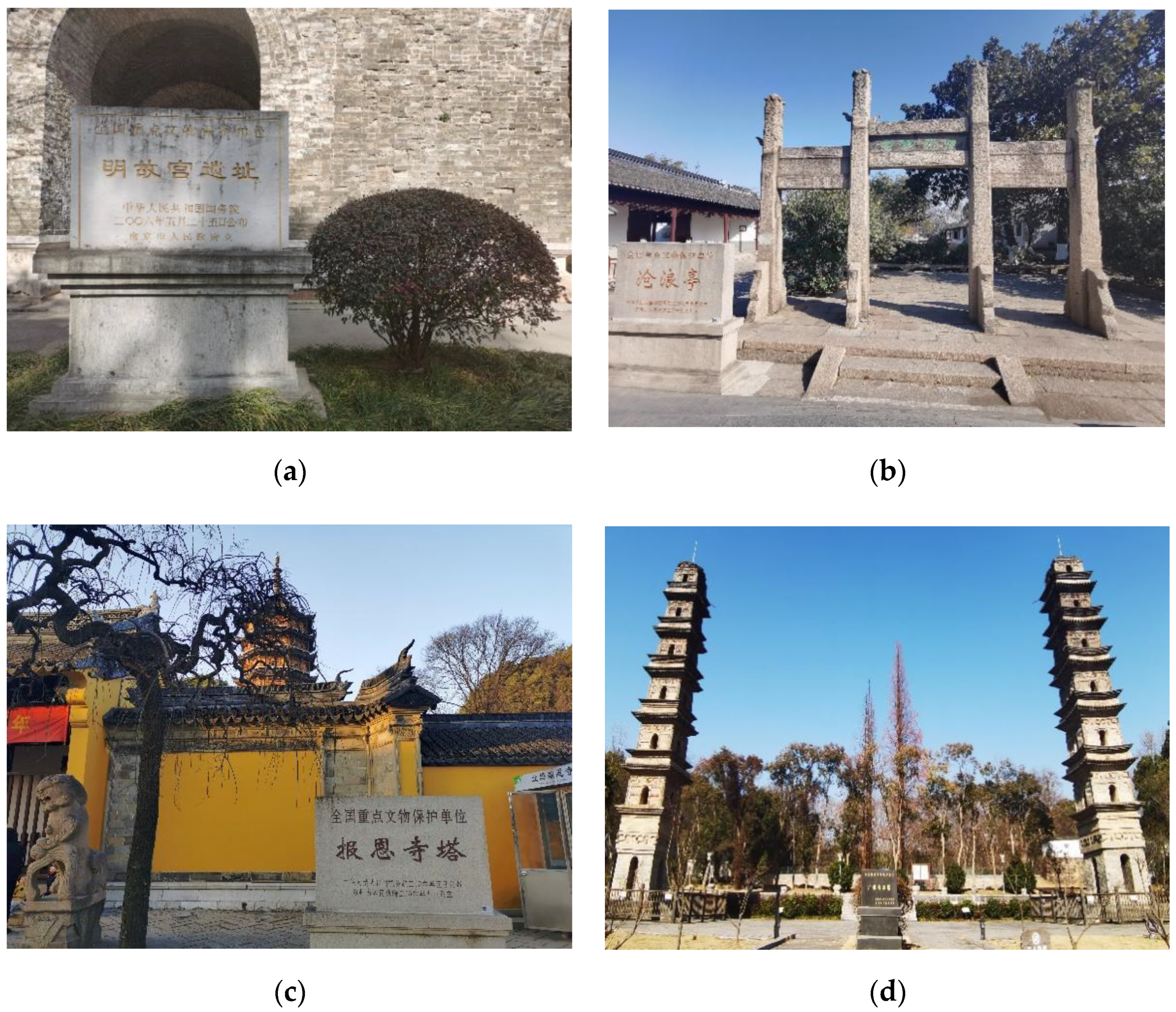
Figure 3.
Examples of Archaeological Sites: (a) The Palace Museum of Ming Dynasty in Nanjing country, (b) The Canglang Pavilion in Suzhou country, (c) The Baoen Temple Pagoda in Suzhou country, (d) The Two pagodas of Guangjiao Temple in Xuancheng country.
Figure 3.
Examples of Archaeological Sites: (a) The Palace Museum of Ming Dynasty in Nanjing country, (b) The Canglang Pavilion in Suzhou country, (c) The Baoen Temple Pagoda in Suzhou country, (d) The Two pagodas of Guangjiao Temple in Xuancheng country.

Figure 4.
Normal distribution diagram.

Figure 5.
The expression of the space-time cube.

Figure 6.
Technical flow chart.

Figure 7.
Spatial autocorrelation results.

Figure 8.
Significant distribution of cold- and hot-spots at Archaeological Sites.

Figure 9.
The space-time cube expression of Archaeological Sites in the study area.

Figure 10.
The space-time cube trend analysis of Archaeological Sites.

Figure 11.
G-STC-M analysis of Archaeological Sites.

Figure 12.
Analysis of space-time cube slices in Archaeological Sites. (a) G-STC-M analysis of Archaeological Sites of Tang and Song Dynasties, (b) G-STC-M analysis of Archaeological Sites of Song and Yuan Dynasties, (c) G-STC-M analysis of Archaeological Sites of Yuan and Ming Dynasties, (d) G-STC-M analysis of Archaeological Sites of Ming and Qing Dynasties.


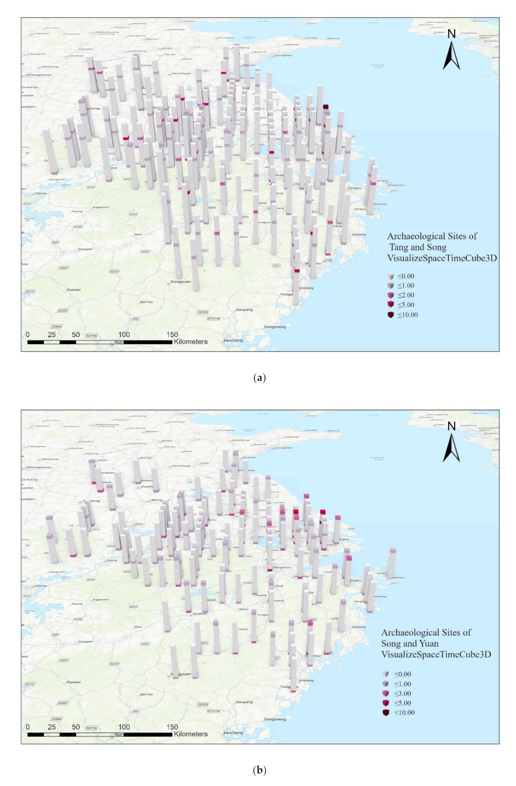
Figure 13.
The space-time cube expression of Archaeological Sites. (a) The space-time cube expression Archaeological Sites of Tang and Song Dynasties, (b) the space-time cube expression Archaeological Sites of Song and Yuan Dynasties, (c) the space-time cube expression Archaeological Sites of Yuan and Ming Dynasties, (d) the space-time cube expression Archaeological Sites of Ming and Qing Dynasties.


Table 1.
Research data introduction.
| Categories | Number | Example |
|---|---|---|
| Ancient cultural sites | 109 | Zicheng site in Jiaxing, Qiyunshan stone carvings |
| Ancient buildings | 1463 | Stone pagoda of lingjiu Temple, Shouxian ancient city wall |
| Ancient tombs | 131 | Tomb of Li Bai, Beishan tombs |
| Stone carvings and grottoes | 112 | Confucius Temple stele forest, Qiyunshan stone carvings |
| Other categories | 30 | Shuanggou old pit group, Jinshan ancient well |
| Some data sources: | http://www.jiangsu.gov.cn/art/2019/4/8/art_64797_8297355.html (accessed on 8 April 2019) | |
| http://www.ah.gov.cn/public/1681/7925731.html (accessed on 9 April 2019) | ||
| http://www.zj.gov.cn/art/2020/12/4/art_1229441734_210.html (accessed on 8 November 2019) | ||
| http://www.shpt.gov.cn/wenhuaju/gkfawen/20200918/523481.html (accessed on 13 April 2016) |
Table 2.
Significant degree of cold- and hot-spots’ clustering.
| Gi_Bin | Z-Score | p-Value | Confidence/(%) | Cold and Hotspots |
|---|---|---|---|---|
| 3 (or −3) | >+2.58 (or <−2.58) | <0.01 | 99 | Hotspots (or cold spots) |
| 2 (or −2) | >+1.96 (or <−1.96) | <0.05 | 95 | Hotspots (or cold spots) |
| 1 (or −1) | >+1.65 (or <−1.65) | <0.1 | 90 | Hotspots (or cold spots) |
| 0 | −1.65 < Z < 1.65 | >0.1 | - | Not statistically significant hot or cold spots |
Table 3.
Space-time cube spatio-temporal scale effect (Distance).
| Distance Interval (km) | Time Interval (Year) | Number of Empty Columns | Z-Score | Number of Cold- and Hot-Spots | Ratio of Cold- and Hot-Spots | Cold- and Hot-Spots Change Ratio |
|---|---|---|---|---|---|---|
| 20 | 50 | 92.32% | 0.6098 | 164 | 27.79% | - |
| 40 | 50 | 89.19% | 0.6098 | 28 | 10.48% | −17.31% |
| 60 | 50 | 86.77% | 0.6098 | 14 | 9.72% | −0.76% |
| 80 | 50 | 84.99% | 0.6098 | 19 | 20.65% | 10.96% |
| 100 | 50 | 83.30% | 0.6098 | 8 | 12.70% | −7.95% |
Table 4.
Space-time cube spatio-temporal scale effect (Time).
| Distance Interval (km) | Time Interval (Year) | Number of Empty Columns | Z-Score | Number of Cold- and Hot-Spots | Ratio of Cold- and Hot-Spots | Cold- and Hot-Spots Change Ratio |
|---|---|---|---|---|---|---|
| 60 | 50 | 86.77% | 0.6098 | 59 | 40.97% | - |
| 60 | 60 | 84.57% | 0.727 | 55 | 38.19% | −2.78% |
| 60 | 70 | 81.48% | 0.7871 | 52 | 36.11% | −2.08% |
| 60 | 80 | 78.53% | 0.8012 | 42 | 29.17% | −6.94% |
| 60 | 90 | 76.74% | 0.8839 | 39 | 27.08% | −2.09% |
Table 5.
Grading table of the variation trend of Archaeological Sites.
| Classification | Z-Score | p-Value | Confidence/(%) | Trend of Change |
|---|---|---|---|---|
| −3 | Z < −2.58 | p < 0.01 | 99 | downward |
| −2 | −2.58 ≤ Z < −1.96 | 0.01 ≤ p < 0.05 | 95 | downward |
| −1 | −1.96 ≤ Z < −1.65 | 0.05 ≤ p < 0.1 | 90 | downward |
| 0 | −1.65 ≤ Z < 1.65 | p ≥ 0.1 | - | no significant trend |
| 1 | 1.65 ≤ Z < 1.96 | 0.05 ≤ p < 0.1 | 90 | upward |
| 2 | 1.96 ≤ Z < 2.58 | 0.01 < p ≤ 0.05 | 95 | upward |
| 3 | Z ≥ 2.58 | p ≤ 0.1 | 99 | upward |
Table 6.
Significant cold- and hot-spots trend classification.
| Model Type | Description |
|---|---|
| New (Cold) Hotspots | The current position is the last time step (cold) hotspot and has not been statistically significantly (cold) hot before |
| Consecutive (Cold) Hotspot | The current position contains statistically significant (cold) hotspots in the last time-step interval and is not continuously uninterrupted, and is not a (cold) hotspot before the last (cold) hotspots, and up to 90% of all bars are statistically significant (cold) hotspots. |
| Intensifying (Cold) Hotspot | The current position is a statistically significant (cold) hotspot for 90% of the time-step interval (including the last time step). In addition, the clustering intensity of each time step showed an increasing trend on the precedent, and the trend was statistically significant. |
| Persistent (Cold) Hotspot | The current location is a statistically significant (cold) hotspot with a 90% time-step interval, and the degree of clustering does not tend to increase or decrease over time. |
| Diminishing (Cold) Hotspot | The current position is the (cold) hotspot with statistical significance of a 90% time-step interval (including the last time step), and the clustering strength of each time step generally presents a decreasing trend, and the trend is statistically significant. |
| Sporadic (Cold) Hotspot | The current position is intermittent (cold) hotspots, and up to 90% of the time-step intervals are statistically significant (cold) hotspots. |
| Oscillating (Cold) Hotspot | A (cold) hotspot of statistical significance for the last time-step interval, and the interval has a history of being a (cold) hotspot in the previous time step. |
| Historical (Cold) Hotspot | The most recent time period is not a (cold) hotspot, but at least 90% of the time-step intervals are statistically significant (cold) hotspots. |
| No Pattern Detected | Does not belong to any of the (cold) hot patterns defined. |
Publisher’s Note: MDPI stays neutral with regard to jurisdictional claims in published maps and institutional affiliations. |
© 2021 by the authors. Licensee MDPI, Basel, Switzerland. This article is an open access article distributed under the terms and conditions of the Creative Commons Attribution (CC BY) license (https://creativecommons.org/licenses/by/4.0/).
Share and Cite
MDPI and ACS Style
Cui, J.; Liu, Y.; Sun, J.; Hu, D.; He, H. G-STC-M Spatio-Temporal Analysis Method for Archaeological Sites. ISPRS Int. J. Geo-Inf. 2021, 10, 312. https://0-doi-org.brum.beds.ac.uk/10.3390/ijgi10050312
AMA Style
Cui J, Liu Y, Sun J, Hu D, He H. G-STC-M Spatio-Temporal Analysis Method for Archaeological Sites. ISPRS International Journal of Geo-Information. 2021; 10(5):312. https://0-doi-org.brum.beds.ac.uk/10.3390/ijgi10050312
Chicago/Turabian StyleCui, Jing, Yanrong Liu, Junling Sun, Di Hu, and Handong He. 2021. "G-STC-M Spatio-Temporal Analysis Method for Archaeological Sites" ISPRS International Journal of Geo-Information 10, no. 5: 312. https://0-doi-org.brum.beds.ac.uk/10.3390/ijgi10050312
Note that from the first issue of 2016, this journal uses article numbers instead of page numbers. See further details here.