
Geospatial Decision-Making Framework Based on the Concept of Satisficing


1
Faculty of Engineering and Sustainable Development, University of Gävle, 80176 Gävle, Sweden
2
Division of Visual Information and Interaction, Department of Information Technology, Uppsala University, 75105 Uppsala, Sweden
*
Author to whom correspondence should be addressed.
ISPRS Int. J. Geo-Inf. 2021, 10(5), 326; https://0-doi-org.brum.beds.ac.uk/10.3390/ijgi10050326
Submission received: 12 March 2021
/
Revised: 30 April 2021
/
Accepted: 8 May 2021
/
Published: 12 May 2021
Abstract
:Decision-making methods used in geospatial decision making are computationally complex prescriptive methods, the details of which are rarely transparent to the decision maker. However, having a deep understanding of the details and mechanisms of the applied method is a prerequisite for the efficient use thereof. In this paper, we present a novel decision-making framework that emanates from the need for intuitive and easy-to-use decision support systems for geospatial multi-criteria decision making. The framework consists of two parts: the decision-making model Even Swaps on Reduced Data Sets (ESRDS), and the interactive visualization framework. The decision-making model is based on the concept of satisficing, and as such, it is intuitive and easy to understand and apply. It integrates even swaps, a prescriptive decision-making method, with the findings of behavioural decision-making theories. Providing visual feedback and interaction opportunities throughout the decision-making process, the interactive visualization part of the framework helps the decision maker gain better insight into the decision space and attribute dependencies. Furthermore, it provides the means to analyse and compare the outcomes of different scenarios and decision paths.
1. Introduction
Providing support for geospatial decision making is one of the main goals of geographic information systems (GIS). GIS-based multi-criteria decision analysis (GIS-MCDA), defined in [1] as “a collection of methods and tools for transforming and combining geographic data and preferences (value judgements) to obtain information for decision making”, emerged during the last couple of decades as a whole new interdisciplinary field of study. There is today a whole plethora of prescriptive multi-criteria decision-making (MCDM) methods and tools that are used for different types of geospatial decision problems. In [1], the most commonly used methods are categorized as either multi-attribute decision-making (MADM) or multi-objective decision-making (MODM) methods. While MADM assumes a finite set of alternatives, MODM deals with design process; the predefined set of alternatives is non-existent and the number of alternatives is continuous, or infinite [2]. Prescriptive methods aim to help decision makers make rational choices and decisions. Making a rational choice means in this context making the optimal choice. Such methods are based on complex computational models that are rarely transparent to the decision maker. The efficiency of these methods ultimately relies on the input given by the decision maker. In order to make a rational choice, giving the right input in itself may demand not only knowledge and information about the issues relevant for the decision problem, but also the knowledge and understanding of how the provided input is processed in a specific method.
Most of the prescriptive decision-making methods used today are implemented through decision-making tools that make only limited use of interactive visualization. In addition, they are often non-transparent and difficult to understand in detail while demanding the decision maker to be able to express their preferences as quantitative relations between criteria. This is partly due to the inherent non-interactivity of the methods [3,4]. This issue was addressed in Andrienko and Andrienko [5], who pointed out that visualization has rather limited use in the design phase and the choice phase of the decision process, and is usually limited to the initial, intelligence phase. Here, the authors use a generalization of the decision-making process proposed in Simon [6], with intelligence, design, and choice as three major phases. The intelligence phase covers the problem definition, data collection, exploration, and preprocessing. The alternatives are defined in the design phase and in the choice phase they are evaluated, whereby the most appropriate alternative or set of alternatives is selected. Informed choice requires the more extensive use of visualization with a high degree of user interactivity in all three phases, thus enabling the decision maker to see how the suggested solution is positioned both in geographical and in attribute space [5].
The models of rational behaviour that are based on the assumption that the deciding subject always tries to make the optimal choice have been questioned by many, most notably Herbert A. Simon [7]. The critics adopted the concept of bounded rationality, according to which our rationality is limited by the incompleteness of available information, our cognitive limitations, and the time available for decision making. Rather than always trying to make the optimal choice, we tend to follow a decision-making process that leads to a satisfactory outcome, and the search stops when a solution is found that satisfies all the conditions. This decision-making model is known as satisficing. The concept of satisficing as a decision-making model was first introduced in Simon [8] as a descriptive model for how people actually make decisions. It describes a multi-criteria decision-making strategy in which the decision maker provides the minimum value of an alternative in terms of each of the considered criteria in order to be considered acceptable (acceptability threshold), and then chooses the first alternative that satisfies the condition.
The aim of this study was to design a framework for geospatial decision making that considers the findings of behavioural decision-making theories, and makes extensive use of interactive visualization throughout the decision process. The main objectives of this work are:
- Develop a decision-making model based on the concept of satisficing;
- Design a visualization framework that incorporates visualization units and interaction paths compatible with the model;
- Create a fully functional decision support tool that integrates the decision-making model and the visualization framework.
2. Related Work
In this section, we present previous work related to each of the research areas relevant for our study. MADM methods commonly used in GIS-MCDM are presented in Section 2.1. Work related to the concept of bounded rationality and the satisficing decision-making model is presented in Section 2.2. Relevant research in the field of interactive visualization in decision making is presented in Section 2.3, and interactive visualization in GIS decision support systems is reviewed in Section 2.4.
2.1. MADM Methods
Depending on the working framework on which they are based, the methods used in the context of GIS-MCDM may be classified as either outranking methods, ideal point methods, or weighted summation methods.
A preference relation among alternatives in outranking methods is usually built by applying the concordance–discordance principle on several attributes. This principle states that an alternative x is not dominated by an alternative y (xSy) if (i) a majority of the attributes supports this assertion; and (ii) the opposition of the attributes which do not is not “too strong” [9]. This relation is constructed through the pairwise comparison of alternatives based on the model of preferences suggested in [10]. The model defines four preference modes: indifference (I), strict preference (P), weak preference (Q), and incomparability (R). A family of multi-criteria decision making known as ELECTRE (Elimination et Choix Traduisant la Réalité (Elimination and Choice Expressing Reality)) is based on this IPQR model. Another popular outranking method is PROMETHEE (Preference Ranking Organization Method for Enrichment of Evaluations) which is often used for group decision making.
In ideal point methods, alternatives are evaluated based on their multidimensional distance to a specific target—ideal point. The core of the ideal point methods lies in the intuitive concept that the chosen alternative should be as close as possible to the hypothetical alternative considered to be the best and as far away as possible from the worst. This hypothetical ideal alternative provides the highest score on each considered criterion. Ideal point methods differ mainly in the applied separation measures, i.e., the way in which they calculate the separation of an alternative to the ideal solution. The most commonly used ideal point method in GIS-MCDM is TOPSIS (Technique for Order of Preference by Similarity to Ideal Solution).
The most common approach in GIS-MCDM decision making is weighted summation, i.e., combining a weighting method and an aggregation method. It includes the following four steps:
- Preparing criteria maps;
- Generating alternatives;
- Deciding relative importance of criteria;
- Creating the overall utility layer.
AHP, which is the most frequently used method for criteria weighting in the context of GIS-MCDM [3], was first introduced in [11]. It relies on decomposing a decision problem into a hierarchy of simpler sub-problems. The method is used to aggregate the relative importance, or priority, on multiple levels. On the top level, the priorities of the criteria are assigned by comparing any two criteria at the time, deciding their relative importance with respect to the main objective. Similarly, if there are any sub-criteria, their priorities with respect to the parent criterion are assigned on the next level and finally, at the bottom level, the priorities are assigned to the alternatives with respect to each criterion. The priorities are assigned in form of a pairwise comparison matrix based on the subjective judgements of the decision maker. Fuzzy AHP, a variant of AHP, uses fuzzy numbers instead of crisp numbers in the comparison ratios [12]. It is often used to minimize the uncertainty related to the subjective judgements. More recently developed criteria weighting models, such as the Best Worst Method (BWM) and Full Consistency Method (FUCOM) attempt to overcome the shortcomings of AHP in terms of consistency and robustness regarding subjectivity. BWM [13,14] and its fuzzy variant FBWM [15,16] use an approach similar to AHP but instead of comparing each criteria with all the others, the decision maker identifies the most important (best) and least important (worst) criteria and then conducts pairwise comparisons between each of these two criteria and the other criteria, significantly reducing the number of comparisons. FUCOM and its fuzzy variant, Fuzzy Full Consistency Method (FUCOM-F), further reduce the number of comparisons to only n-1, and yield more consistent results than both AHP and BWM [17,18].
2.2. Bounded Rationality and the Satisficing Model
The concept of satisficing as a decision-making model was first introduced in Simon [8] as a descriptive model for how people actually make decisions. It describes a multi-criteria decision-making strategy in which the decision maker provides the minimum value of an alternative in terms of each of the considered criteria (acceptability threshold) and then chooses the first alternative that satisfies the condition. The satisficing model is based on the concept of bounded rationality, presented in Simon [7] (although the term bounded rationality is first used in Simon [19]). Simon questions proposed models of rational behaviour that are based on the assumption that the deciding subject always tries to make the optimal choice. In order for a choice to be considered rational according to these models, the deciding subject needs to perform complex analyses and computations, such as determining the pay-off function for each possible outcome, calculating the probability that a certain outcome will ensue when a certain alternative is chosen, etc. These tasks, according to Simon, are not, and indeed cannot be, performed in actual choice situations due to cognitive limitations and the lack of time. The model suggested by the author implies that we, instead of performing overly complex computations to obtain an “optimal” outcome, tend to perform a simpler decision-making process which leads to a satisfactory outcome. Satisficing is used as a stop rule, and the search stops when “a solution has been found that is good enough along all dimensions” [20]. Gigerenzer [21] introduced the notion of adaptive toolbox as a framework for bounded rationality. Adaptive toolbox is defined as a set of heuristics modelled “on the actual cognitive abilities a species has, rather than on the imaginary powers of omniscient demons”. These heuristics are designed for domain-specific goals, enabling fast and computationally simple decisions. They also allow human beings to deal with high uncertainty, where we cannot know the probabilities and/or consequences of different outcomes [22].
A notion of maximizing expected utility as a criterion of rational decision making has been further criticized in Klein [23]. Based on the analysis of the boundary conditions for optimizing decisions, compiled from the assumptions made in the literature, Klein concludes that decision makers will be unable to optimize in field settings, as the requirements are too restrictive to be applicable outside laboratory settings [23]. A recent work by Lieder and Griffiths suggests, however, that although human decision making deviates from expected utility theory, those deviations should not be seen as an indication of human irrationality but rather as a reflection of people’s rational use of limited cognitive resources [24,25].
The concept of satisficing as a model for behavioural decision making has been evaluated in a number of studies. Gigerenzer and Goldstein [26] performed a study where a number of algorithms based on the concept of satisficing, such as the “Take The Best” algorithm, were compared with more rational inference procedures. Despite its counter-intuitive name that suggests optimization, the “Take The Best” algorithm is a basic satisficing algorithm that only searches through a portion of the total knowledge (information) and stops immediately when the first discriminating cue (criterion) is found. The basic algorithm that discriminates between two alternatives is in Gigerenzer and Goldstein [26] described as a five-step process:
- Recognition principle: If only one of the two objects (alternatives) is recognized, choose that object. If neither of the two objects are recognized, make a random choice. Otherwise, proceed to step two;
- Search for cue values: Retrieve from memory the cue values for the highest ranking cue (criterion);
- Discrimination rule: Decide whether the cue discriminates between the alternatives;
- Cue-substitution principle: If the cue discriminates, stop search. Otherwise, go back to step 2 and continue with the next cue;
- Maximizing rule: Choose the object with the positive cue value, or choose randomly if no cue discriminates.
The authors found that the “Take The Best” algorithm matched, and in some cases, even outperformed more rational inference procedures such as multiple regression. Satisficing and the theory of bounded rationality were investigated in Agosto [27] in relation to young people’s decision making in the World Wide Web. The results showed that participants in the study in general made their decisions in accordance with the satisficing model. The two major satisficing behaviours, namely reduction and termination, were observed during the study. Reduction was demonstrated as relying on and returning to known sites, and termination as stopping the search after the acceptable outcome was found. Zhu and Timmermans [28] proposed a modelling framework for shopping behaviour incorporating the principles of bounded rationality. The framework implements models based on three basic heuristic rules (conjunctive, disjunctive and lexicographic rule), extended with a threshold heterogeneity (probabilistically distributed thresholds). These heuristic models were estimated and compared with multinomial logit models on four decision situations: go home, choose direction, rest and choose preferred store. The results of the comparison showed that the heuristic models were superior to the multinomial in all four modelled decision situations. Nakayama and Sawaragi [29] developed the Satisficing Trade-off Method, a decision-making method based on satisficing, as an alternative to computationally and cognitively complex interactive multi-objective optimization methods. The first step in their five-step method is setting the ideal point that remains fixed throughout the process. In step two, the decision maker sets the aspiration levels for all attributes. In step three, a set of acceptable solutions is obtained by the Min–Max method. The trade-offs are performed in step four, where the decision maker classifies the criteria into three groups: the criteria to be improved more, the criteria that may be relaxed, and the criteria which are accepted as they are. The new acceptable levels of criteria are set in this step. Finally, in step five, a feasibility check is performed. The results of the performed tests showed that the method was very effective for problems with a large number of objective functions and expensive auxiliary optimization.
Although Simon’s theory of bounded rationality has been widely recognized, it seems to have had little influence on the development of decision-making models and methods. Jankowski [30] notes that the development of prescriptive decision models and methods shifted the focus from theoretic concepts of decision making towards algorithmic and computational aspects of modelling. Decision theory has been marginalized in prescriptive models, which often adopt a utility maximizing stance. This applies not least to spatial decision support systems and GIS where, despite the findings in the field of behavioural decision making, the rational model of decision making persisted as a theoretical construct used in normative models [30].
2.3. Interactive Visualization in Decision Making
The development of human insight is aided by interaction with a visual interface, and Pike et al. [31] see this as the central percept of visual analytics. Even though interactive features are present in virtually every visualization tool regardless of the application area, little attention has been paid to interaction [32] and it receives little emphasis in visualization research [33]. This seemingly contradictory claim is based on the observation that most of the research related to interaction is concerned with the analysis and design of the user interface rather than the interaction itself. Beaudouin-Lafon [34] pointed out that user interfaces are the means and not the end of interaction. We need to be concerned with designing the interaction, rather than interfaces, to control the quality of the interaction between the user and computer. In what he called the Visual Information Seeking Mantra, Shneiderman summarized the basic principle of interaction design as “Overview first, zoom and filter, then details-on-demand” [35]. The issue of interaction design is addressed in Yi et al. [32], where the authors proposed the following seven general categories of interaction techniques used in information visualization: select, explore, reconfigure, encode (alter the visual representation), abstract/elaborate, filter, and connect (highlight relationships between data items). Rather than being organized around the low-level interaction techniques provided by the system, these categories are organized around a user’s intent while interacting with the system. Users’ intent, as well as preferences and competence, are also important parts of the suggested guidelines for visualization recommendation systems—systems that can identify and recommend visualizations relevant for a specific task—suggested in Vartak et al. [36]. Other factors relevant for guidelines are data characteristics (correlations, patterns and trends, etc.), semantics and domain knowledge, and visual ease of understanding. In accordance with the recommendations, the quality of visualization is to be judged by relevance for the task, surprise (relevant visualization that the user has not asked for), non-obviousness, diversity, and coverage. Elmqvist et al. [33] explained the skewed balance between the visual and the interactive aspects of visualization in visualization research by the inherent intangibility of the concept of interaction, that is difficult to design, quantify, and evaluate. Based on the analysis of existing visualizations with efficient interactive features, the authors suggest practical interaction design guidelines which they call fluid interaction. A fluid interface (i) promotes flow (a mental state of immersion in an activity); (ii) supports direct manipulation based on continuous representation of the objects, physical actions instead of complex syntax, and rapid and reversible operations with immediately visible impact; and (iii) minimizes the difference between the state of the system and the user’s perception of it, as well as the difference between the allowable actions and user’s intentions.
2.4. Interactive Visualization in GIS Decision Support Systems
The importance of interactivity in geospatial decision support systems can hardly be overstated. Factors such as the complexity and multi-dimensionality of data, large number of alternatives, and uncertainty regarding input data and/or expected outcomes set high demands on the design and efficiency of the visualization framework and its interaction features. The negative impact of interface complexity on geospatial decision making has been identified in a number of studies. The results of the study presented in Vincent et al. [37] showed that, when using interactive maps to improve spatial decision making, interface complexity influenced decision outcomes more than the decision complexity. Moreover, participants made better decisions using the simpler interface. A related issue of complexity of the representation methods was investigated in Cheong et al. [38]. In the study, participants were given different representations of uncertainty. The results showed that there is little difference in the decision-making performance between groups if there is enough time to focus on the problem. Under time pressure, however, participants using simpler representation models performed better than the participants using more advanced cartographic representations. Andrienko and Andrienko [39] addressed the issue of complexity of geospatial decision support tools. There is a tendency to design generic systems that will be applicable to many types of data sets and which address the needs of many different users. This leads to complex systems that are difficult to use. Instead, the authors suggested that systems should be designed in accordance with the concept of a sufficient minimum, i.e., systems should be capable of recognizing which instruments make a minimum combination appropriate to analyse a specific data collection and simplify itself accordingly. The development in the area of interactive visualization as a support for geospatial decision making has more recently led to a number of novel methods and tools. These include generic tools [40,41,42,43], as well as tools aimed towards specific tasks, such as the interpretation and understanding of the impact of simulated flood risks [44,45,46], watershed simulation [47], exploring socio-economic vulnerability [48], geospatial network of actors [49], marine pollution monitoring [50], the transnational flow of hazardous waste [51], monitoring climate change [52], prediction and the analysis of genomic islands [53], and many more. Most of the task-specific geospatial decision support systems developed during the last four or five years are Web GIS systems, i.e., client–server systems where the server is either a dedicated GIS server or a custom server application, and where the client is a web browser. Elwood and Leszczynski [54] refer to Web GIS systems as new spatial media that enable everyday users, not only experts, to access and engage in the decision-making process. In a way, Web GIS democratizes geospatial decision making, and the trend of using the Internet as a primary platform for GIS systems is likely to continue.
3. Method
Satisficing is introduced as a descriptive model for a behavioural multi-criteria decision-making strategy that is actually deployed when we make decisions. According to this strategy, the decision maker provides the minimum value of an alternative in terms of each of the considered criteria (acceptability threshold) and then chooses the first alternative that satisfies the condition. This implies that the decision process is sequential, and that the final choice will depend on the order in which the alternatives are evaluated [55]. However, Malczewski and Ogryczak [56] argued that, even if an individual behaves in accordance with satisficing principles of rationality, they still have some tendency towards maximizing utility. Malczewski and Rinnner [1] referred to this type of behaviour as quasi-satisficing rationality. According to this principle, the decision maker should identify the most preferred alternative from the set of remaining acceptable solutions, irrespective of the attainability or aspiration levels. The Even Swaps on Reduced Data Sets (ESRDS) model presented here adopted this view and provides the means of further evaluating the alternatives that satisfy all the conditions in order to select a single most preferred alternative. Furthermore, ESRDS is based on the idea of interactive multi-objective programming methods, according to which the most preferred alternative is to be determined through a progressive communication process between the decision maker and the application. This procedure is in Malczewski and Rinnner [1] described as consisting of two phases: the dialogue phase, in which the decision maker analyses information and articulates their preferences; and the computational phase, in which a solution or set of solutions is generated. This interaction is continued until an outcome is considered acceptable by the decision maker.
The starting point of ESRDS is the formal statement of the normative satisficing procedure given in MacCrimmon [55]:
Suppose a set of minimal attribute values is defined on . An alternative j is satisfactory only if for all i. An unsatisfactory alternative —that is, an alternative for which for some —is dropped from consideration.
The model upon which the decision-making framework presented in this work was based is explained in Section 3.1. In Section 3.2, we give an overview of the features of the visualization framework.
3.1. ESRDS Decision-Making Model
At the beginning of a decision process, the acceptability threshold for each criterion is set to the minimum value that an alternative has in terms of that particular criterion:
Thus, all alternatives in the set are considered acceptable. When the acceptability threshold for criterion is adjusted, all alternatives in the set that have the value in terms of lower than the acceptability threshold are discarded from the set. The set of valid alternatives A is then defined as
where is the value of in terms of the criterion . By adjusting the acceptability thresholds of all criteria, the user is able to reduce the number of alternatives as only the alternatives conforming to all the acceptability thresholds are kept in the set. The process of adjusting acceptability thresholds is iterative, i.e., the decision maker can repeatedly tighten or loosen the threshold for any of the criteria in order to reduce or increase the set of acceptable alternatives. An important feature of ESRDS is the automatization of the threshold update process. This feature may be used at any stage as long as there is at least one criterion where . However, it is best used after the set of valid alternatives has been reduced to a manageable size by adjusting the acceptability threshold manually, and we want to further analyse the decision space by exploring dependencies between pairs of criteria, while keeping the size of the set of alternatives unchanged.
The threshold update automatization used in ESRDS aims to provide an interactive tool for what-if analysis. In a typical scenario, the user chooses a criterion, , that will respond to an adjustment in another criterion . Ideally, when the acceptability threshold for the criterion is changed by x units, there is a value y such that, when the threshold value for is changed by y units, the total number of valid alternatives, , remains unchanged. However, it is not always possible to find y that will generate a set of alternatives of size . Assume that and the decision maker increases the threshold for , , so that only 30 alternatives are left in A. The threshold for , , needs to be decreased so that 20 alternatives that have previously been filtered out by the higher value of are added to the set. In reality, it might be the case that decreasing by some value c generates 18 new alternatives, and decreasing it by gives 23 new alternatives. In such cases, our algorithm chooses y that gives the smallest possible value of d, where d is the difference between and ; in this case, and :
Through an iterative process, the decision maker sets and adjusts the threshold values for the criteria and analyses intermediate results. When the decision maker is content with the set of alternatives obtained by the process, the dominated alternatives are removed from the set. An alternative is said to be dominated by an alternative if it is inferior to on at least one criterion and not superior to on any other criteria:
where is the value of in terms of criterion k.
Finally, from the set of the alternatives which conform to the decision maker’s aspirations, the most preferred alternative is selected by applying even swaps. Even swaps is a trade-off-based method for multiple criteria decision making under certainty. The essence of the issue of trade-offs under certainty is described in Keeney and Raiffa [57] as “How much achievement on objective 1 is the decision maker willing to give up in order to improve achievement on objective 2 by some fixed amount?”. As an iterative method based on dimensionality reduction, even swaps was first introduced in Hammond et al. [58]. In Hammond et al. [59], it is defined by the following five steps:
- Determine the change necessary to cancel out criterion R;
- Assess what adjustments need to be done in another criterion, M, in order to compensate for the needed change;
- Make even swap. An even swap is a process of increasing the value of an alternative in terms of one criterion and decreasing the value by an equivalent amount in terms of another. After the swaps are performed over the whole range of alternatives, all alternatives will have the same value on R and it can be cancelled out as irrelevant in the process of ranking the alternatives;
- Cancel out the now-irrelevant criterion R;
- Eliminate the dominated alternative(s).
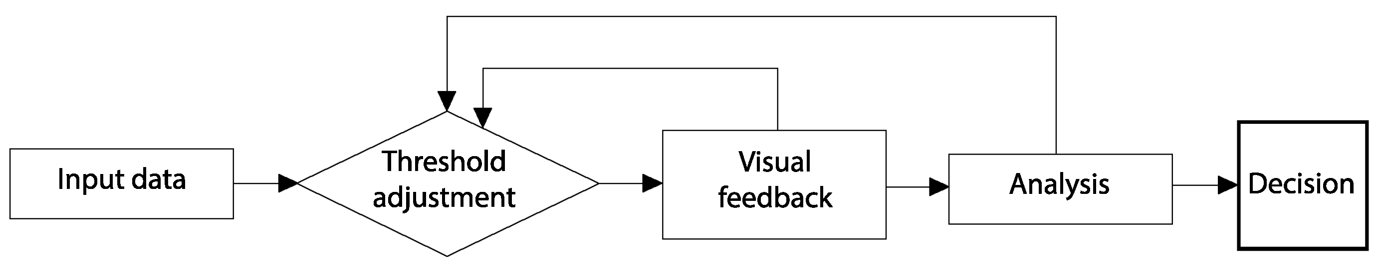
The process pipeline for the decision-making model is presented in Figure 1.
3.2. Visualization Framework
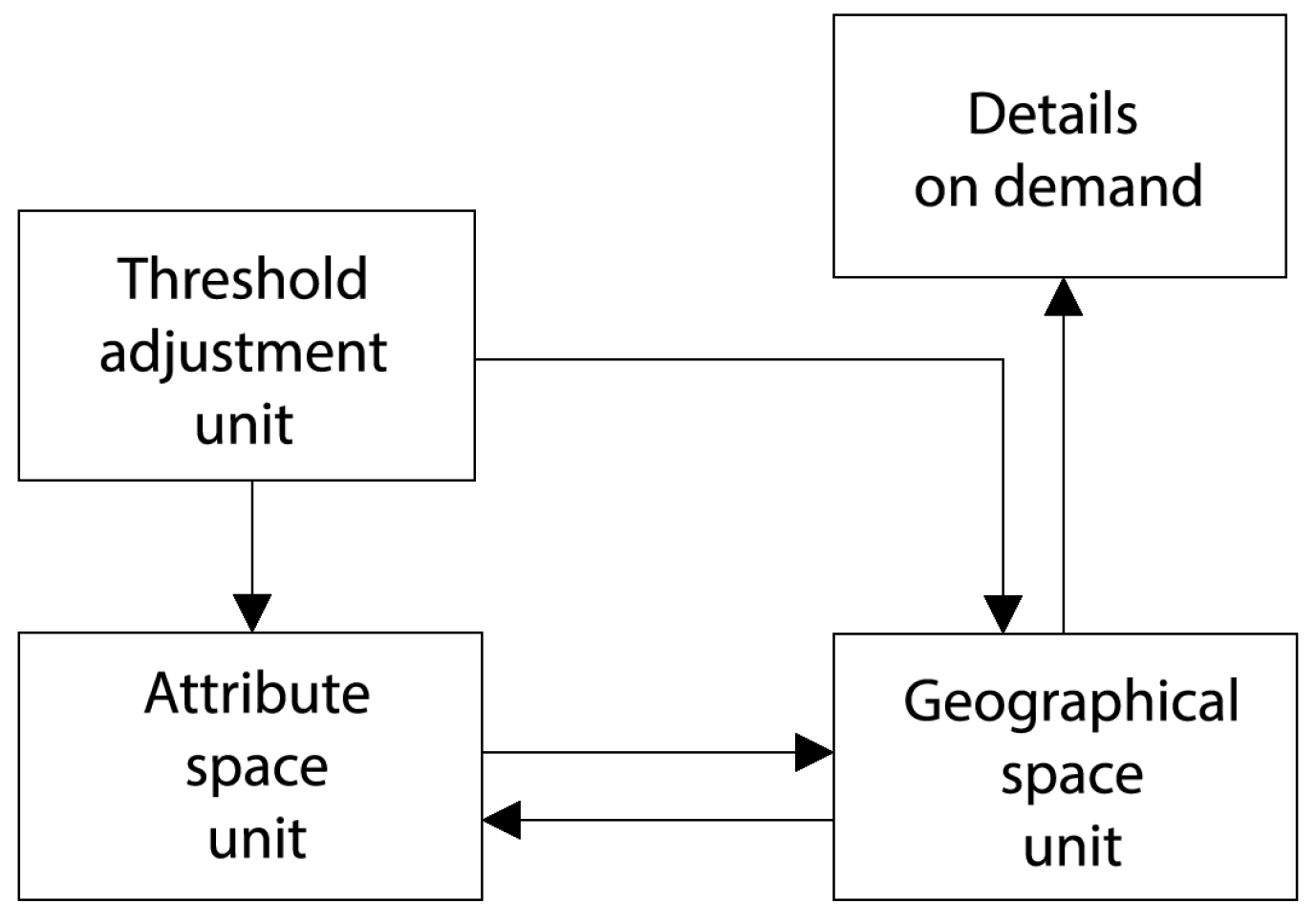
The decision-making framework presented in this paper emerged from the recognition of the necessity of integrating algorithmic techniques and visualization in order to create sophisticated interactive tools for GIS-MCDM [60,61]. It follows the principle suggested in Keim et al. [61], which states that in any analytical process, the user has to be the ultimate authority in directing the analysis, and that the system must provide effective means of interaction that will facilitate the user in any specific task. Visualization features of the framework are designed to give the user full insight into the decision space, both in the attribute and in the geographical space, as well as means of isolating and analysing a limited part of the decision space. The visualization framework presented here includes the following three units:
- Threshold adjustment unit. This is the core interaction unit, in which the user adjusts threshold values for the criteria. The direct result of an adjustment is shown for the adjusted criterion and every other criterion, if affected. The unit panel contains sliders for threshold adjustments for each of the criteria. For each criterion, a histogram is provided that shows the distribution of the values in terms of that particular criterion;
- Attribute space analysis unit. This panel is shown when the set of acceptable alternatives is reduced to a manageable level. A parallel coordinates plot is used to visualize the relations between the remaining acceptable alternatives in attribute space;
- Geographical space analysis unit. A geomap is used for visualization of the positions of the acceptable alternatives in geographical space;
The interaction path between different units is given in Figure 2.
4. Result
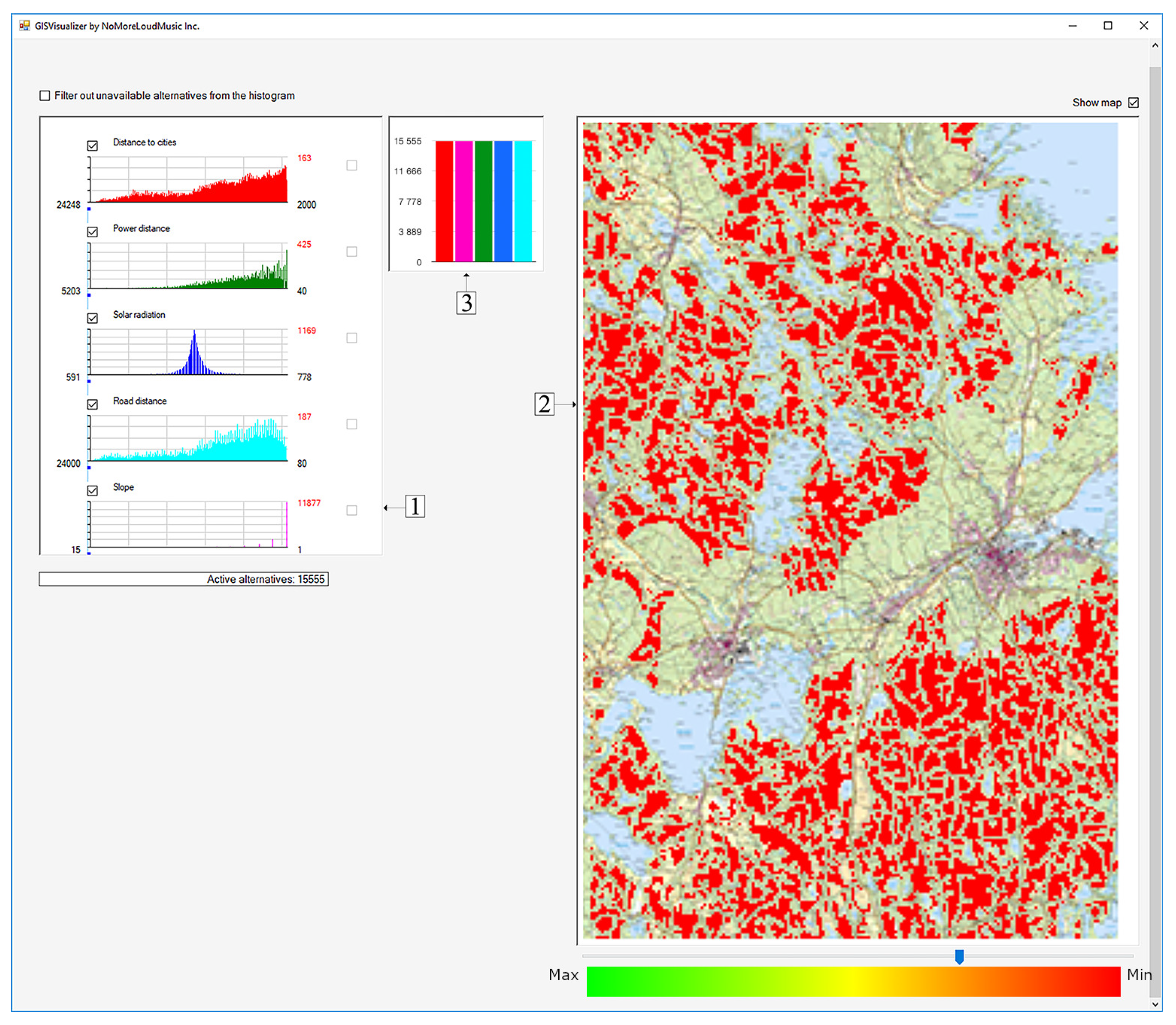
In order to demonstrate the proposed framework, we developed GISAnalyzer, a decision support tool that implements the model and the visualization framework presented in Section 3. The initial setup is shown in Figure 3.
The application takes input for each criterion from an ESRI ASCII grid file. Each file contains values of the alternatives in terms of one particular criterion, i.e., the number of input files corresponds to the number of criteria. After loading the input data, the main window containing the threshold adjustment panel (Figure 3, 1) and the map panel (Figure 3, 2) are shown. The threshold adjustment panel is shown with default settings, where the threshold value for each criterion is set to the minimum value that an alternative has in terms of that particular criterion. Values of the alternatives in terms of each of the criteria are obtained by scaling the nominal values to a 0–255 scale. For the more, the better type of criteria, alternatives with highest nominal values have the value 255 and alternatives with lowest nominal values have the value 0. The opposite applies to the less, the better criteria. The geographic map is shown with all acceptable alternatives, which in the initial setup means all alternatives coded red. This is due to the fact that the colour coding in the map changes depending on which criterion is currently manipulated. Since none of the criteria are initially selected, the colour coding in the map does not consider the values, but only the geographic positions of the alternatives. A bar chart visualization of the number of alternatives conforming to the acceptability threshold value for each of the criteria serves as a complement to the threshold adjustment panel (Figure 3, 3).
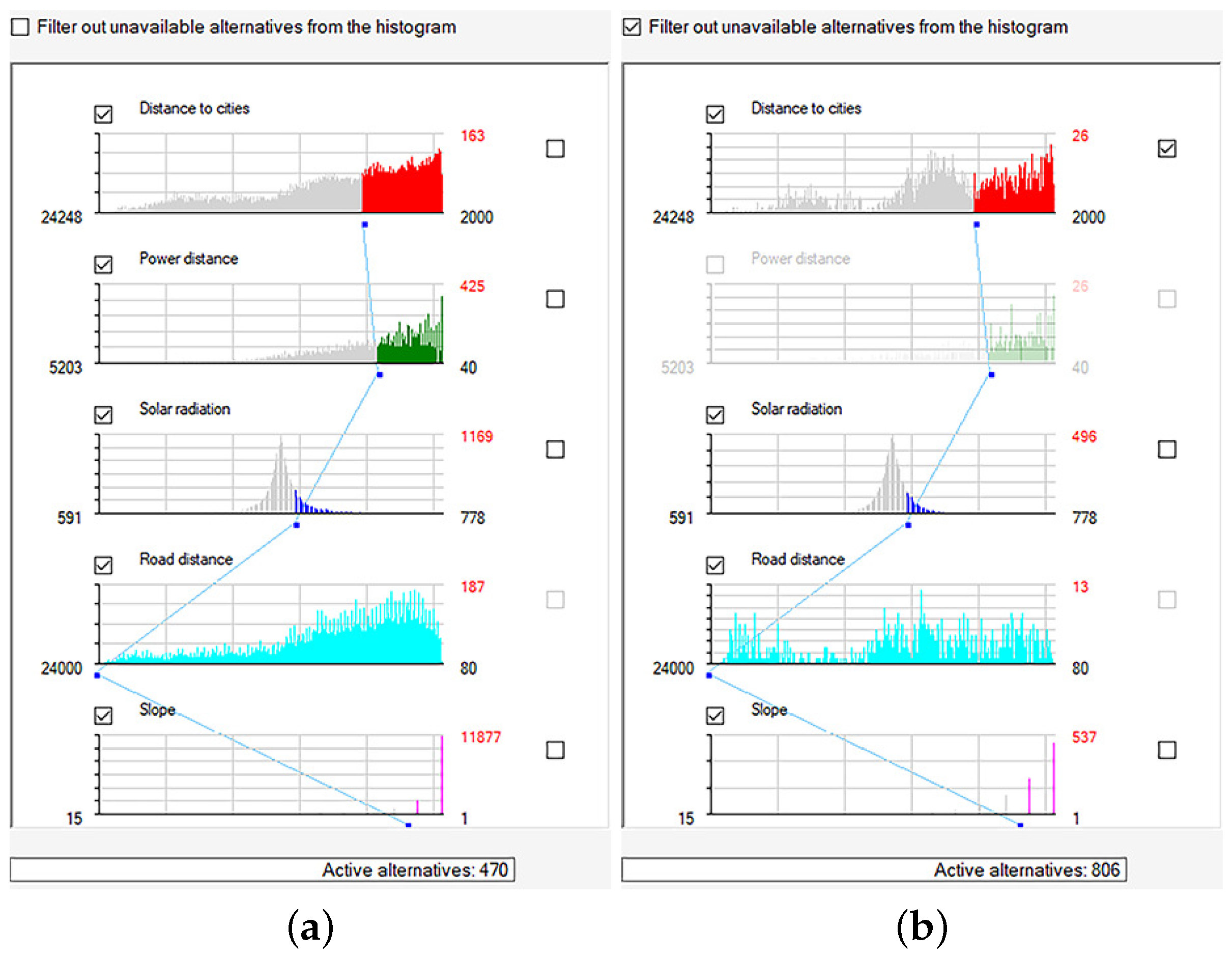
The main unit of the application is the threshold adjustment unit. The threshold for each criterion is adjusted with a slider, and a histogram is used to represent the distribution of the values of the alternatives in terms of each of the criteria. When the threshold is adjusted for any of the criteria, the histogram is updated and the part filtered out by the change is coloured light grey. Throughout the adjustment process, the user can choose either non-filtered or filtered adjustment panel view. In the non-filtered view (Figure 4a), the histogram for a particular criterion concerns all alternatives conforming to the threshold value for that particular criterion, regardless of whether they are acceptable or not (whether or not they conform to all thresholds). In the filtered view, the histogram only concerns the acceptable alternatives (Figure 4b). If the user wants to discard a certain criterion, this can be done by unchecking the criterion. The current acceptability threshold is saved, and the criterion is excluded from the calculations until it is checked again. When a threshold for at least one criterion is set to a value larger than , the option for automatized adjustment is made available. The user can use any criterion as the adjusting criterion (), but only a criterion with can be chosen as the one to be automatically adjusted ().
In the geomap, the currently acceptable alternatives (each alternative is represented by a pixel in the map) are colour-coded from red to green based on the value in terms of the criterion whose threshold is currently being adjusted. The alternatives with the lowest value are coded red and the alternatives with the highest value are coded green. One example is given in Figure 5.
In some cases, when the number of remaining acceptable alternatives is small and the alternatives are spread over the wider area, it may be difficult to see them on the map, especially if the map colour at the area where the alternatives are drawn is similar to the colour-coding of the alternatives. In such cases, the user has an option to show a desaturated map. Then, the alternatives, as they remain coloured, protrude in contrast to the desaturated map, making it easier for the decision maker to see their placement (Figure 6).
When the number of remaining acceptable alternatives is less than a predefined limit , the attribute space panel is shown. The values of the alternatives in terms of each of the criteria are shown in a parallel coordinates plot (Figure 7).
This plot is drawn with axes, where n is the number of criteria. The other two axes represent the longitude and latitude, respectively, of the alternatives in the map, i.e., they mirror the geographic location of the alternatives. In GISAnalyzer, we chose to make the plot visible but non-interactive for , where is the number of acceptable alternatives, is the maximum number of alternatives to be shown in the plot, and is the maximum number of alternatives for which the plot interaction is enabled. While the plot still may be understood and interpreted for up to several hundred alternatives (polylines), selecting a single polyline, which is a precondition for an interactive feature, may be difficult and virtually impossible in a plot with too many polylines. When the interactive feature is enabled, all acceptable alternatives are marked in the geomap. The interaction between the map and the plot is bidirectional. When a polyline is selected, the corresponding alternative is encircled in the map. If an alternative is selected (clicked on) in the geomap, the corresponding polyline is highlighted in the plot. Selecting an alternative in the geomap provides detailed information, which consists of textual information regarding the values in terms of each of the criteria for the selected alternative, as well as a bar chart (Figure 8a). The bar chart gives a hint of the overall value of an alternative by presenting the portion of the maximum value in terms of each of the criteria for the alternative in question. The user may select an area in the map, in which case polylines corresponding to all acceptable alternatives within the area are highlighted (Figure 8b). Bar charts for the selected alternatives in this scenario are not available.
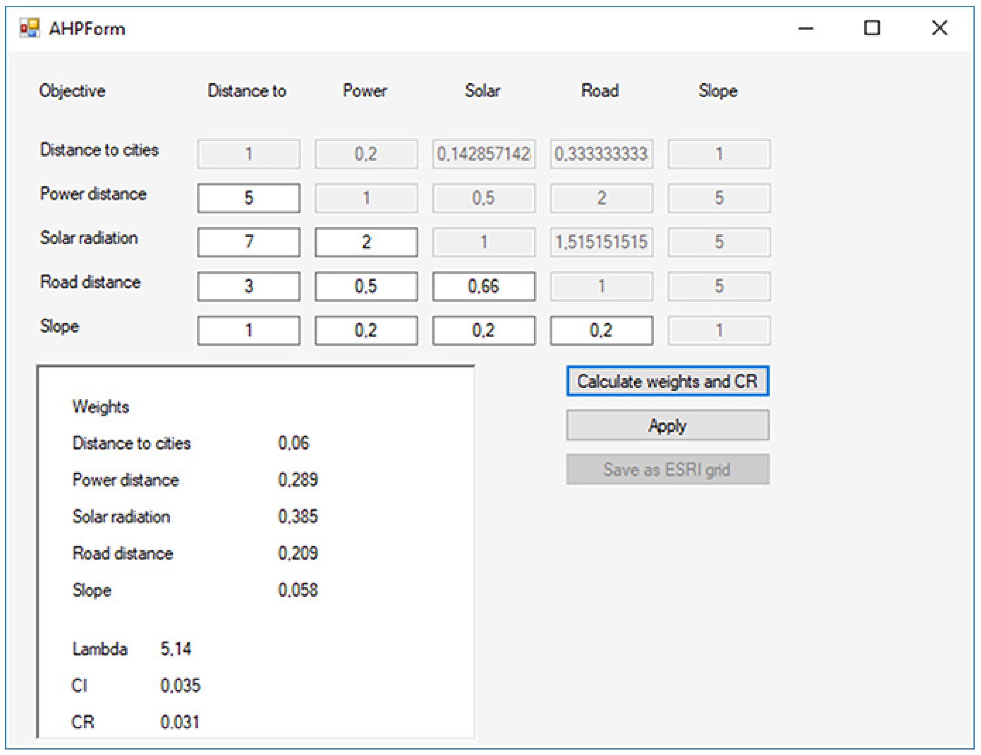
In GISAnalyzer, we implemented a comparison feature which adds further possibilities for a thorough analysis during the decision process, and we chose AHP as the comparison method. Even though we are critical of the AHP method for its many shortcomings, not least in the way it is used in GIS-MCDM, it is the most frequently used decision-making method in geospatial decision making, and thus most likely to be familiar to a user. It is important to emphasize that AHP is not an integral part of our framework, but an extra feature of GISAnalyzer. After the user has performed an analysis and obtained a final set of acceptable alternatives A, the comparison feature may be used to compare the results with the results of handling the problem with AHP. The AHP functionality implemented in the application cannot be used for the complete hierarchical AHP process, but only to assign weights to the criteria (Figure 9).
For , the set of highest ranked alternatives obtained by AHP applies that (the number of alternatives in is equal to the number of alternatives in A) and . The polyline for each alternative in is added to the parallel coordinates plot. For the number of polylines after adding, , applies that . in cases when there are no common alternatives to AHP and the threshold adjustment, and in the opposite case, when the sets obtained by AHP and the threshold adjustment are identical.
When the AHP is functionality is enabled, each polyline is colour-coded depending on which of the following conditions is met:
- : magenta;
- : cyan;
- : colour-coded from red to green based on the value of , where is the alternative represented by the polyline, n is the number of criteria, and is the value of in terms of the criterion .
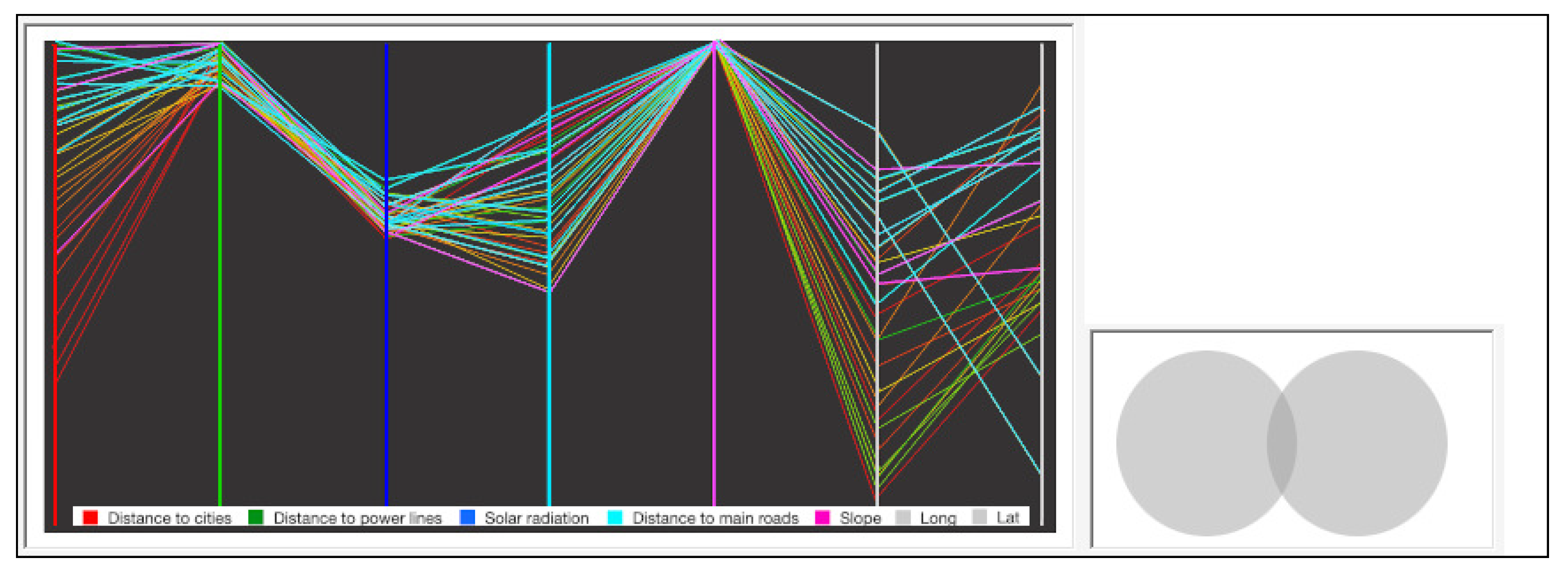
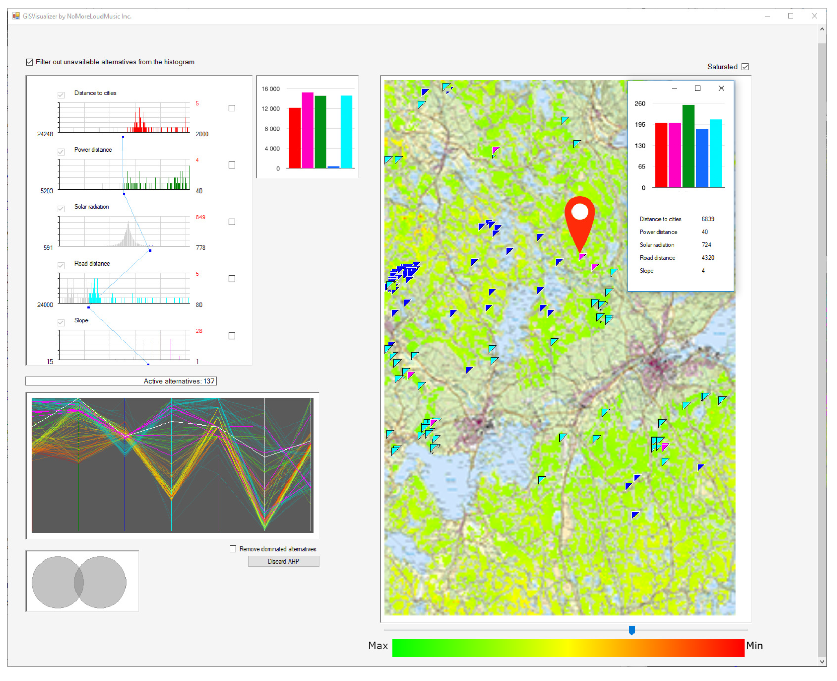
The portion of alternatives satisfying the condition is visualized by means of a complementary diagram as the intersection of two circles representing A and , respectively. It applies that , where is the intersection area, is the area of one of the circles, , and k is the number of elements of the set . The parallel coordinates plot and the complementary diagram are shown in Figure 10. If the criteria weights are changed, i.e., if the changes are made in the preference matrix in the AHP window, is updated and the parallel coordinates plot, the complementary diagram, and the geomap are refreshed with the current values.
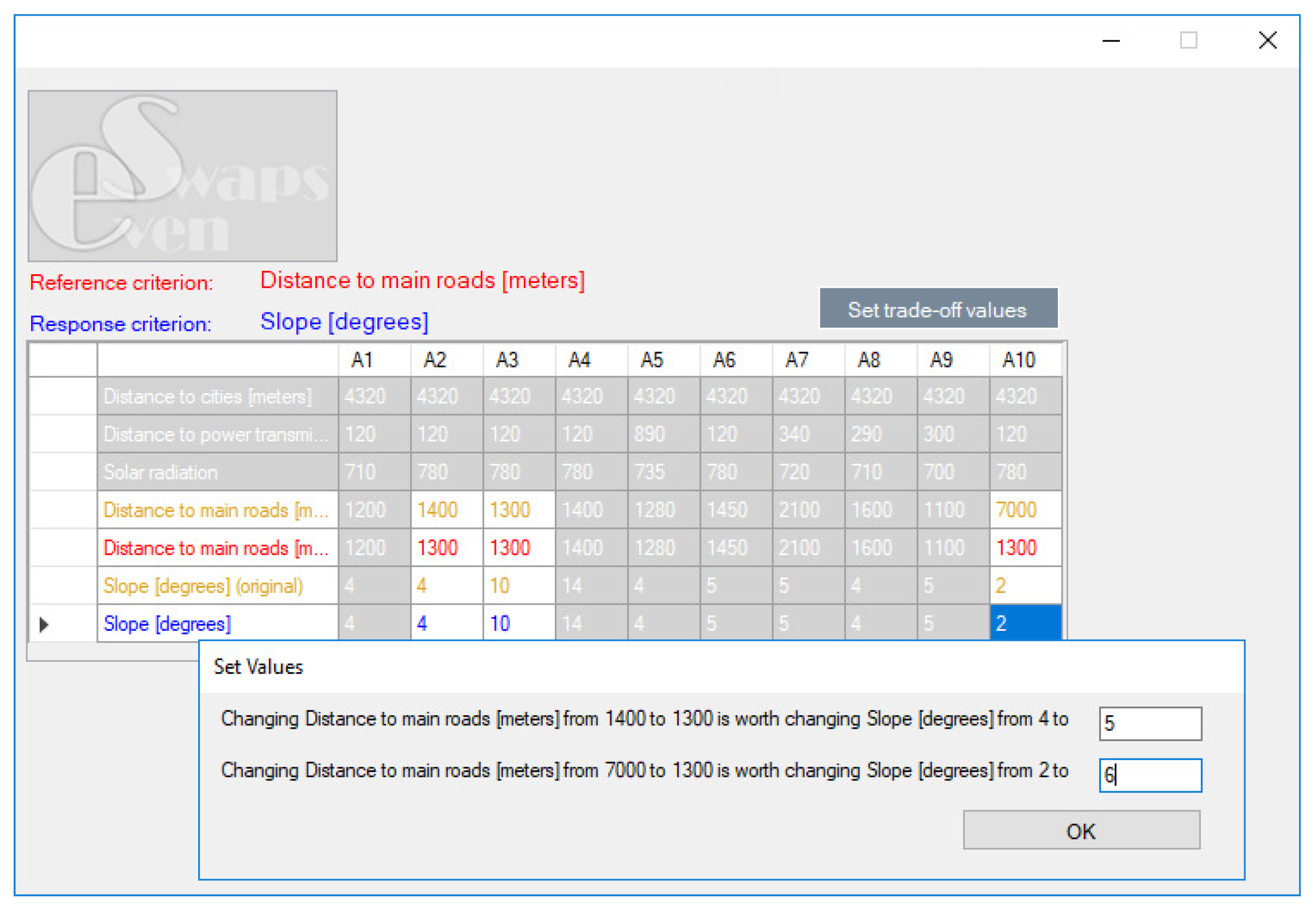
When the number of available alternatives is equal to or less than a predefined maximum number of alternatives which is manageable by even swaps, the even swaps feature is available to the decision maker. Even swaps opens in a separate window, where the decision maker performs swaps. After each turn, the application removes dominated alternatives, if there are any, and dismisses the reference criterion from further process. An example of applying even swaps on a hypothetical solar farm site location decision problem with five criteria is given in Figure 11. The full view of the application main window after applying even swaps as well as the AHP comparison feature is shown in Figure 12.
5. Discussion and Conclusions
In this paper, we presented a novel decision-making framework that emanates from the need for intuitive and easy-to-use decision support systems for geospatial multi-criteria decision making that will serve both expert and non-expert users. It is based on the concept of satisficing; however, instead of fully adopting satisficing as the stop rule, the proposed framework implements a quasi-satisficing model. This still allows the decision maker to choose any alternative from the set of alternatives that satisfy all the conditions. At the same time, it provides the option to apply even swaps upon the set of acceptable alternatives, in order to choose the most preferred alternative.
Based on the pairwise comparison of alternatives, the even swaps method is not applicable to geospatial decision problems in quasi-continuous choice models with large numbers of alternatives. In [3] we presented GISwaps, a new method for geospatial decision making based on even swaps which uses virtual alternatives that are representative for the whole decision space in order to interpolate the compensation values needed to compensate for adjustments in the reference criterion for all alternatives. The satisficing-based approach deployed in the present study relies on an iterative data reduction process which enables the use of the even swaps method in its basic form in geospatial decision making. Including the even swaps method into our decision-making framework adds to its applicability and efficiency while it does not significantly increase its complexity, as even swaps in itself is a rather intuitive method based on trade-offs, is easy to understand and is reasonably easy to apply.
Compared to the established models used in GIS-MCDM—weighted summation methods, outranking methods, and ideal point methods—the advantage of ESRDS is two-fold: (1) it can handle an almost unlimited number of alternatives; and (2) it does not rely on criteria weighting. In the context of GIS-MCDM, the decision space is usually represented in a quasi-continuous choice model, with the number of alternatives limited only by the resolution of the digital model of the geographic area of interest. Under such conditions, analysis and pairwise comparison between alternatives is not feasible, as it would require comparisons for n alternatives. Weighted summation, outranking, and ideal point methods all deploy criteria weighting at some stage, which is not problematic when the number of alternatives is small. In GIS-MCDM, however, assigning weights to criteria associated with map layers is usually done without considering the values of the actual alternatives—a mistake known in decision theory as the most common critical mistake [57]. Suppose that we want to buy a house and we choose between house A which costs USD 100,000, house B which costs USD 150,000, and house C which costs USD 200,000. Obviously, price would be a very if not probably the most important factor. However, if the prices were USD 100,000 for house A, USD 105,000 for house B, and USD 110,000 for house C, we would probably consider price to be much less relevant.
The comparison between the different models (Table 1), in terms of the number of alternatives they can manage, assumes correct usage of criteria weighting, i.e., judging the importance of criteria considering the values of alternatives. In terms of handling uncertainty, ESRDS, just as the remaining compared models, assumes that outcomes and consequences are known in advance, i.e., it is not suitable for decision making under uncertainty.
The interactive visualization, which is an integral part of the framework, enables the efficient use of ESRDS in the geospatial context. It provides visual feedback on the decision maker’s every action throughout the decision process in two different views that represent the attribute and the geographical space, respectively. This, in combination with the detail-on-demand feature, gives the decision maker the opportunity to analyse and compare the outcomes of different scenarios and decision paths. Furthermore, the available means of interaction help the decision maker gain insight in attribute dependencies and discover the potential relations between the criteria that would otherwise remain hidden.
The presented framework and GISAnalyzer that implements it are results of the effort to incorporate the findings in the field of behavioural decision making into a prescriptive decision model. The framework will be evaluated in a future study, focusing on two main issues: how efficient is the proposed model in the context of GIS-MCDM, and to what extent does the interactive visualization facilitate the decision maker in learning about and better understanding the decision problem.
Author Contributions
Conceptualization, Goran Milutinović; Methodology, Goran Milutinović; Software, Goran Milutinović; Supervision, Stefan Seipel and Ulla Ahonen-Jonnarth; Visualization, Goran Milutinović; Writing–original draft, Goran Milutinović; Writing–review & editing, Ulla Ahonen-Jonnarth. All authors have read and agreed to the published version of the manuscript.
Funding
This research received no external funding.
Conflicts of Interest
The authors declare no conflict of interest.
References
- Malczewski, J.; Rinner, C. Multicriteria Decision Analysis in Geographic Information Science; Springer Science + Business Media: Berlin/Heidelberg, Germany, 2015. [Google Scholar]
- Zavadskas, E.K.; Turskis, Z.; Kildienė, S. State of art surveys of overviews on MCDM/MADM methods. Technol. Econ. Dev. Econ. 2014, 20, 165–179. [Google Scholar] [CrossRef] [Green Version]
- Milutinovic, G.; Ahonen-Jonnarth, U.; Seipel, S. GISwaps—A New Method for Decision Making in Continuous Choice Models Based on Even Swaps. Int. J. Decis. Support Syst. Technol. 2018, 10, 57–78. [Google Scholar] [CrossRef] [Green Version]
- Milutinovic, G.; Seipel, S. Visual GISwaps—An Interactive Visualization Framework for Geospatial Decision Making. In Proceedings of the 13th International Joint Conference on Computer Vision, Imaging and Computer Graphics Theory and Applications, Madeira, Portugal, 27–29 January 2018; SCITEPRESS: Setubal, Portugal, 2018; Volume III, pp. 236–243. [Google Scholar]
- Andrienko, N.; Andrienko, G. Informed spatial decisions through coordinated views. Inf. Vis. 2003, 2, 270–285. [Google Scholar] [CrossRef]
- Simon, H.A. New Science of Management Decision; Harper: New York, NY, USA, 1960. [Google Scholar]
- Simon, H.A. Behavioral Model of Rational Choice. Q. J. Econ. 1955, 69, 99–118. [Google Scholar] [CrossRef]
- Simon, H.A. Rational choice and the structure of the environment. Psychol. Rev. 1956, 63, 129–138. [Google Scholar] [CrossRef] [Green Version]
- Bouyssou, D. Outranking methods. In Encyclopedia of Optimization, Volym 1; Christodoulos, F.A., Panos, P.M., Eds.; Springer: Berlin/Heidelberg, Germany, 2009; pp. 249–255. [Google Scholar]
- Roy, B. The outranking approach and the foundations of electre methods. Theory Decis. 1991, 31, 49–73. [Google Scholar] [CrossRef]
- Saaty, T. The Analytic Hierarchy Process; McGraw-Hill: New York, NY, USA, 1980. [Google Scholar]
- Buckley, J.J. Fuzzy hierarchical analysis. Fuzzy Sets Syst. 1985, 17, 233–247. [Google Scholar] [CrossRef]
- Rezaei, J. Best-worst multi-criteria decision-making method. Omega 2015, 53, 49–57. [Google Scholar] [CrossRef]
- Liang, F.; Brunelli, M.; Rezaei, J. Consistency issues in the best worst method: Measurements and thresholds. Omega 2020, 96, 102175. [Google Scholar] [CrossRef]
- Guo, S.; Zhao, H. Fuzzy best-worst multi-criteria decision-making method and its applications. Knowl. Based Syst. 2017, 121, 23–31. [Google Scholar] [CrossRef]
- Karimi, H.; Sadeghi-Dastaki, M.; Javan, M. A fully fuzzy best–worst multi attribute decision making method with triangular fuzzy number: A case study of maintenance assessment in the hospitals. Appl. Soft Comput. 2020, 86, 105882. [Google Scholar] [CrossRef]
- Pamučar, D.; Stević, Ž.; Sremac, S. A New Model for Determining Weight Coefficients of Criteria in MCDM Models: Full Consistency Method (FUCOM). Symmetry 2018, 10, 393. [Google Scholar] [CrossRef] [Green Version]
- Pamučar, D.; Ecer, F. Prioritizing the weights of the evaluation criteria under fuzziness: The fuzzy full consistency method—fucom-f. Facta Univ. Ser. Mech. Eng. 2020, 18, 419–437. [Google Scholar]
- Simon, H.A. Models of Man; John Wiley: New York, NY, USA, 1957. [Google Scholar]
- Simon, H.A. Models of Thought; Yale University Press: New Haven, CT, USA, 1979. [Google Scholar]
- Gigerenzer, G. The adaptive toolbox. In Bounded Rationality: The Adaptive Toolbox; Gigerenzer, G., Selten, R., Eds.; The MIT Press: Cambridge, MA, USA, 2001; pp. 37–50. [Google Scholar]
- Maldonato, N.M.; Chiodi, A.; Di Corrado, D.; Esposito, A.M.; De Lucia, S.; Sperandeo, R.; Muzii, B. Heuristics, abductions and adaptive algorithms: A toolbox for human decision making. In Proceedings of the 11th IEEE International Conference on Cognitive Infocommunications, CogInfoCom, Online. 23–25 September 2020; pp. 273–282. [Google Scholar]
- Klein, G. The Fiction of Optimization. In Bounded Rationality: The Adaptive Toolbox; Gigerenzer, G., Selten, R., Eds.; The MIT Press: Cambridge, MA, USA, 2001; pp. 103–121. [Google Scholar]
- Lieder, F.; Griffiths, T.L. Resource-rational analysis: Understanding human cognition as the optimal use of limited computational resources. Behav. Brain Sci. 2020, 43, 1–60. [Google Scholar] [CrossRef] [PubMed] [Green Version]
- Mohnert, F.; Pachur, T.; Lieder, F. What’s in the Adaptive Toolbox and How Do People Choose From It? Rational Models of Strategy Selection in Risky Choice. In Proceedings of the 41st Annual Conference of the Cognitive Science Society, Montreal, QC, Canada, 24–27 July 2019; pp. 2378–2384. [Google Scholar]
- Gigerenzer, G. Reasoning the fast and frugal way: Models of bounded rationality. Psychol. Rev. 1996, 103, 650–669. [Google Scholar] [CrossRef] [Green Version]
- Agosto, D.E. Bounded rationality and satisficing in young people’s web-based decision making. J. Am. Soc. Inf. Sci. Technol. 2002, 53, 16–27. [Google Scholar] [CrossRef]
- Zhu, W.; Timmermans, H. Modeling pedestrian shopping behavior using principles of bounded rationality: Model comparison and validation. J. Geogr. Syst. 2011, 13, 101–126. [Google Scholar] [CrossRef]
- Nakayama, H.; Sawaragi, Y. Satisficing Trade-Off Method for Multiobjective Programming and its Applications. IFAC Proc. Vol. 1984, 17, 1345–1350. [Google Scholar] [CrossRef]
- Jankowski, P. Behavioral decision theory in spatial decision-making models. In Handbook of Behavioral and Cognitive Geography; Montello, D.R., Ed.; Edward Elgar Publishing: Cheltenham, UK, 2018; pp. 41–55. [Google Scholar]
- Pike, W.A.; Stasko, J.T.; Chang, R.; O’Connell, T.A. The science of interaction. Inf. Vis. 2009, 8, 263–274. [Google Scholar] [CrossRef]
- Yi, J.S.; Kang, Y.; Stasko, J.T.; Jacko, J.A. Toward a Deeper Understanding of the Role of Interaction in Information Visualization. IEEE Trans. Vis. Comput. Graph. 2007, 13, 1224–1231. [Google Scholar] [CrossRef] [Green Version]
- Elmqvist, N.; Moere, A.V.; Jetter, H.-C.; Carnea, D.; Reiterer, H.; Jankun-Kelly, T.J. Fluid interaction for information visualization. Inf. Vis. 2011, 10, 327–340. [Google Scholar] [CrossRef]
- Beaudouin-Lafon, M. Designing interaction, not interfaces. In Proceedings of the Working Conference on Advanced Visual Interfaces, Gallipoli, Italy, 25–28 May 2004; pp. 15–22. [Google Scholar]
- Shneiderman, B. The eyes have it: A task by data type taxonomy for information visualizations. In Proceedings of the 1996 IEEE Symposium on Visual Languages, Boulder, CO, USA, 3–6 September 1996; pp. 336–343. [Google Scholar]
- Vartak, M.; Huang, S.; Siddiqui, T.; Madden, S.; Parameswaran, A. Towards Visualization Recommendation Systems. ACM SIGMOD Rec. 2017, 45, 34–39. [Google Scholar] [CrossRef]
- Vincent, K.; Roth, R.E.; Moore, S.A.; Huang, Q.; Lally, N.; Sack, C.M.; Nost, E.; Rosenfeld, H. Improving spatial decision making using interactive maps: An empirical study on interface complexity and decision complexity in the North American hazardous waste trade. Environ. Plan. B Urban Anal. City Sci. 2018, 46, 1706–1723. [Google Scholar] [CrossRef] [Green Version]
- Cheong, l.; Bleisch, S.; Kealy, A.; Tolhurst, K.; Wilkening, T.; Duckham, M. Evaluating the impact of visualization of wildfire hazard upon decision-making under uncertainty. Int. J. Geogr. Inf. Sci. 2016, 30, 1377–1404. [Google Scholar] [CrossRef] [Green Version]
- Andrienko, N.; Andrienko, G. The Complexity Challenge to Creating Useful and Usable Geovisualization Tools. In Proceedings of the Geographic Information Science: Fourth International Conference, Münster, Germany, 20–23 September 2006; pp. 23–27. [Google Scholar]
- Hamilton, M.C.; Nedza, J.A.; Doody, P.; Bates, M.E.; Bauer, N.L.; Voyadgis, D.E.; Fox-Lent, C. Web-based geospatial multiple criteria decision analysis using open software and standards. Int. J. Geogr. Inf. Sci. 2016, 30, 1667–1686. [Google Scholar] [CrossRef]
- Arciniegas, G.; Janssen, R.; Rietveld, P. Effectiveness of collaborative map-based decision support tools: Results of an experiment. Environ. Model. Softw. 2013, 39, 159–175. [Google Scholar] [CrossRef]
- Nair, L.R.; Saleem, S.; Shetty, D. Scalable Interactive Geo Visualization Platform for GIS Data Analysis. In Proceedings of the 2016 IEEE 14th Intl Conf on Dependable, Autonomic and Secure Computing, 14th Intl Conf on Pervasive Intelligence and Computing, 2nd Intl Conf on Big Data Intelligence and Computing and Cyber Science and Technology Congress, Auckland, New Zealand, 8–12 August 2016; pp. 886–889. [Google Scholar]
- Zhang, M.; Wang, H.; Lu, Y.; Li, T.; Guang, Y.; Liu, C.; Edrosa, E.; Li, H.; Rishe, N. TerraFly GeoCloud. ACM Trans. Intell. Syst. Technol. 2015, 6, 1–24. [Google Scholar] [CrossRef]
- Leskens, J.G.; Kehl, C.; Tutenel, T.; Kol, T.; de Haan, G.; Stelling, G.; Eisemann, E. An interactive simulation and visualization tool for flood analysis usable for practitioners. Mitig. Adapt. Strateg. Glob. Chang. 2017, 22, 307–324. [Google Scholar] [CrossRef] [Green Version]
- Aye, Z.C.; Jaboyedoff, M.; Derron, M.H.; Van Westen, C.J.; Hussin, H.Y.; Ciurean, R.L.; Frigerio, S.; Pasuto, A. An interactive web-GIS tool for risk analysis: A case study in the Fella River basin, Italy. Nat. Hazards Earth Syst. Sci. 2016, 16, 85–101. [Google Scholar] [CrossRef] [Green Version]
- Waser, J.; Konev, A.; Adransky, B.; Horváth, Z.; Ribičic, H.; Carnecky, R.; Kluding, P.; Schindler, B. Many plans: Multidimensional ensembles for visual decision support in flood management. Comput. Graph. Forum 2014, 33, 281–290. [Google Scholar] [CrossRef]
- Zhang, S.; Xia, Z.; Wang, T. A real-time interactive simulation framework for watershed decision making using numerical models and virtual environment. J. Hydrol. 2013, 493, 95–104. [Google Scholar] [CrossRef]
- Kienberger, S.; Hagenlocher, M.; Delmelle, E.; Casas, I. A WebGIS tool for visualizing and exploring socioeconomic vulnerability to dengue fever in Cali, Colombia. Geospat. Health 2013, 8, 313–316. [Google Scholar] [CrossRef] [Green Version]
- Nagel, T.; Duval, E.; Vande Moere, A. Interactive exploration of geospatial network visualization. In Proceedings of the 2012 ACM Annual Conference on Human Factors in Computing Systems, Kherson, Ukraine, 6–10 June 2012. [Google Scholar]
- Kulawiak, M.; Prospathopoulos, A.; Perivoliotis, L.; Łuba, M.; Kioroglou, S.; Stepnowski, A. Interactive visualization of marine pollution monitoring and forecasting data via a Web-based GIS. Comput. Geosci. 2010, 36, 1069–1080. [Google Scholar] [CrossRef]
- Nost, E.; Rosenfeld, H.; Vincent, K.; Moore, S.A.; Roth, R.E. HazMatMapper: An online and interactive geographic visualization tool for exploring transnational flows of hazardous waste and environmental justice. J. Maps 2017, 13, 14–23. [Google Scholar] [CrossRef] [Green Version]
- Herring, J.; VanDyke, M.S.; Cummins, R.G.; Melton, F. Communicating Local Climate Risks Online Through an Interactive Data Visualization. Environ. Commun. 2017, 11, 90–105. [Google Scholar] [CrossRef]
- Dhillon, K.B.; Laird, M.R.; Shay, J.A.; Winsor, G.L.; Lo, R.; Nizam, F.; Pereira, S.K.; Waglechner, N.; McArthur, A.G.; Langille, M.g.I.; et al. IslandViewer 3: More flexible, interactive genomic island discovery, visualization and analysis. Nucleic Acids Res. 2015, 43, 104–108. [Google Scholar] [CrossRef]
- Elwood, S.; Leszczynski, A. New spatial media, new knowledge politics. Trans. Inst. Br. Geogr. 2013, 38, 544–559. [Google Scholar] [CrossRef]
- MacCrimmon, K.R. Decisionmaking Among Multiple-Attribute Alternatives: A Survey and Consolidated Approach; RAND Corporation: Santa Monica, CA, USA, 1968. [Google Scholar]
- Malczewski, J.; Ogryczak, W. The Multiple Criteria Location Problem: 2. Preference-Based Techniques and Interactive Decision Support. Environ. Plan. A Econ. Space 1996, 28, 69–98. [Google Scholar] [CrossRef] [Green Version]
- Keeney, R.L.; Raiffa, H. Decisions with Multiple Objectives—Preferences and Value Tradeoffs; John Wiley & Sons: Hoboken, NJ, USA, 1976. [Google Scholar]
- Hammond, J.S.; Keeney, R.L.; Raiffa, H. Even Swaps: A Rational Method for Making Trade-offs. Harv. Bus. Rev. 1998, 76, 137–149. [Google Scholar]
- Hammond, J.S.; Keeney, R.L.; Raiffa, H. Smart Choices—A Practical Guide to Making Better Life Decisions; Broadway Books: New York, NY, USA, 1999. [Google Scholar]
- Sacha, D.; Zhang, L.; Sedlmair, M.; Lee, J.A.; Peltonen, J.; Weiskopf, D.; North, S.C.; Keim, D.A. Visual Interaction with Dimensionality Reduction: A Structured Literature Analysis. IEEE Trans. Vis. Comput. Graph. 2017, 23, 241–250. [Google Scholar] [CrossRef] [Green Version]
- Andrienko, G.; Andrienko, N.; Schumann, H.; Tominski, C.; Demsar, U.; Dransch, D.; Dykes, J.; Fabrikant, S.; Jern, M.; Kraak, M.-J. Space and Time. In Mastering the Information Age: Solving Problems with Visual Analytics; Keim, D., Kohlhammer, J., Ellis, G., Mansmann, F., Eds.; Eurographics Association: Munich, Germany, 2010; pp. 57–86. [Google Scholar]
Figure 1.
The process model for the framework.

Figure 2.
The interaction path between different units of the framework.

Figure 3.
The main window of GISAnalyzer; initial setup, after the data for all criteria are loaded.
Figure 3.
The main window of GISAnalyzer; initial setup, after the data for all criteria are loaded.

Figure 4.
Different views of the threshold adjustment panel: (a) non-filtered view, where, for each criterion, all alternatives conforming to the threshold value for that particular criterion are drawn; (b) filtered view, where only alternatives conforming to all the thresholds are drawn, with one criterion (Power distance) discarded (equivalent to setting the threshold for that criterion to ) and another criterion (Distance to cities) selected as the criterion to be automatically adjusted, . Red numbers in the upper right corner of each histogram denote the number of alternatives with a given value.

Figure 5.
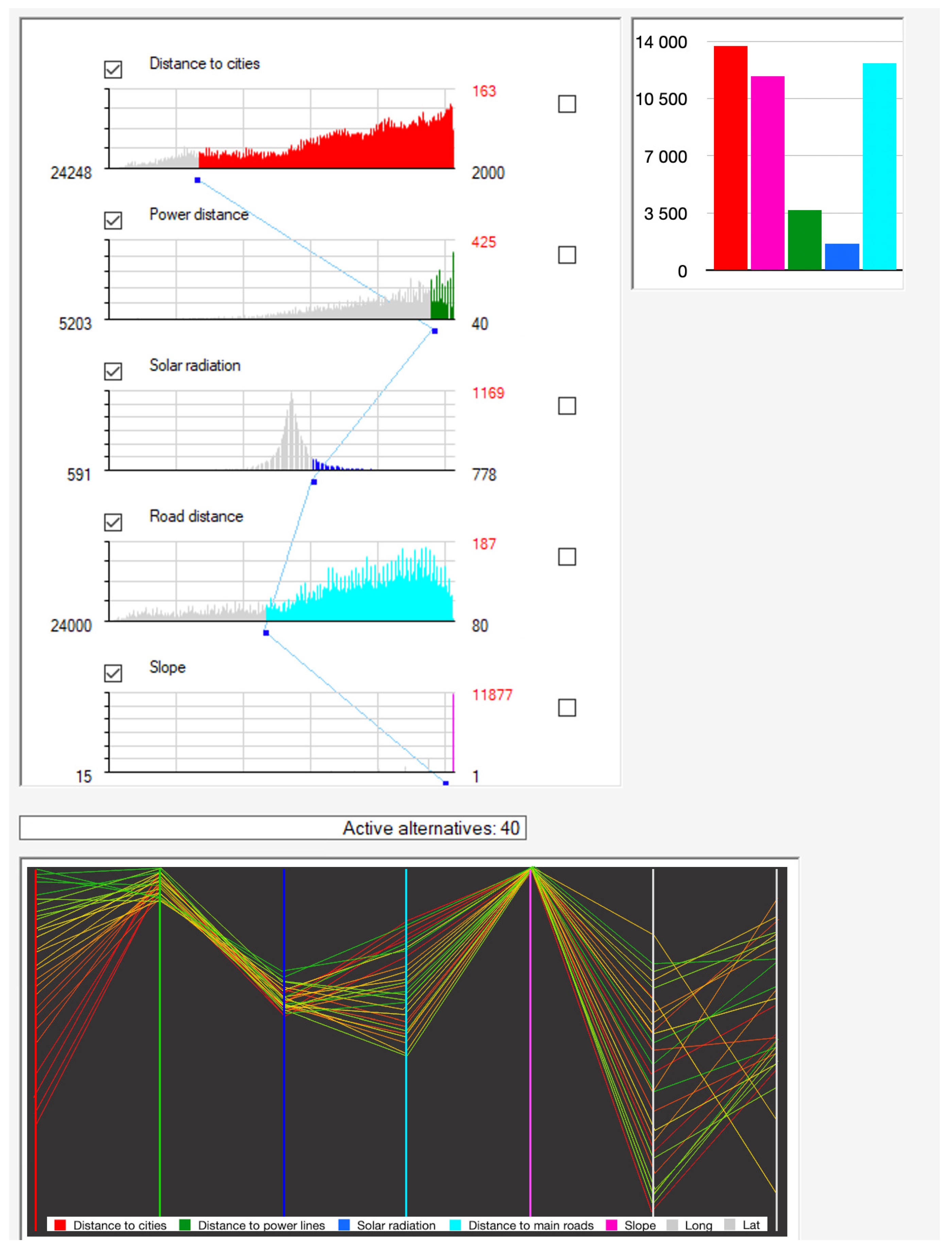
The main application window during the threshold adjustment process. The initial set of 15,555 alternatives is reduced to 4898, by adjusting the thresholds values for three criteria. The threshold for Distance to cities is increased to approximately 8500 m, the threshold for Power distance to approximately 1100 m, and the threshold for Road distance to approximately 14,000 m. The remaining acceptable alternatives are colour-coded based on the value in terms of Road distance, as it happens to be the criterion currently being adjusted.
Figure 5.
The main application window during the threshold adjustment process. The initial set of 15,555 alternatives is reduced to 4898, by adjusting the thresholds values for three criteria. The threshold for Distance to cities is increased to approximately 8500 m, the threshold for Power distance to approximately 1100 m, and the threshold for Road distance to approximately 14,000 m. The remaining acceptable alternatives are colour-coded based on the value in terms of Road distance, as it happens to be the criterion currently being adjusted.

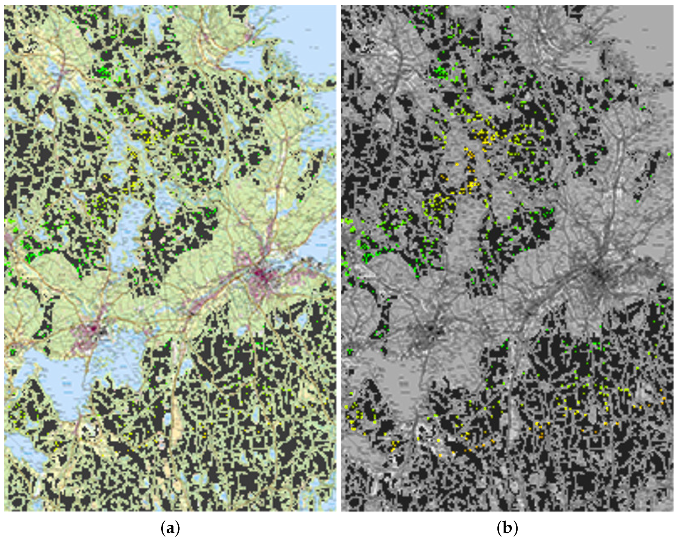
Figure 6.
Geomap in default view (a) and in desaturated view (b).

Figure 7.
Each of the five coloured axes in the parallel coordinates plot holds the values of the remaining acceptable alternatives in terms of one of the criteria. The last two axes represent longitude and latitude of the alternatives in the geographical space. Polylines representing the alternatives are colour-coded from green (best) to red (worst).

Figure 8.
The interaction between the parallel coordinates plot and the geomap. When an alternative is selected in the plot, it is highlighted in the geomap. Selecting the alternative in the geomap opens a “detail-on-demand” window (a). When an area is selected in the geomap, all acceptable alternatives within the selected area are highlighted white in the parallel coordinates plot (b).

Figure 9.
AHP window. The “Apply” button is enabled if the relative importance values for the criteria are consistent, i.e., if the consistency index .
Figure 9.
AHP window. The “Apply” button is enabled if the relative importance values for the criteria are consistent, i.e., if the consistency index .

Figure 10.
The parallel coordinates plot and the complementary diagram after applying comparison with AHP.
Figure 10.
The parallel coordinates plot and the complementary diagram after applying comparison with AHP.

Figure 11.
The status after three of the criteria were previously dismissed from further process and seven dominated alternatives were removed. In the current step, Distance to main roads is chosen as the reference criterion, and Slope is chosen as the response criterion. The values in terms of the response criterion need to be adjusted in order to compensate for the adjustments needed to render all three remaining alternatives equal (at the value of 1300) in terms of the reference criterion. This is done by increasing the value in terms of Slope from four to five degrees for alternative A2, and from two to six degrees for alternative A10. After this swap is performed, the reference criterion, Distance to main roads, will be dismissed. The values in terms of the only remaining criterion, Slope, will be five degrees for A2, ten degrees for A3, and six degrees for A10. A2 is chosen as the most preferred alternative, as it has the best value on the only remaining criterion.

Figure 12.
The full view of the GISAnalyzer main window after applying even swaps to obtain the most preferred alternative.
Figure 12.
The full view of the GISAnalyzer main window after applying even swaps to obtain the most preferred alternative.


Table 1.
Comparison between ESRDS and ranking, ideal point, and weighted summation methods used in GIS-MCDM.
Table 1.
Comparison between ESRDS and ranking, ideal point, and weighted summation methods used in GIS-MCDM.
| Method | Nr. of Alternatives | Criteria Weighting | Handles Uncertainty |
|---|---|---|---|
| ESRDS | Large | No | No |
| Weighted summation methods | Small | Yes | No |
| Outranking methods (ELECTRE, PROMETHEE) | Small | Yes | No |
| Ideal point methods (TOPSIS) | Small | Yes | No |
Publisher’s Note: MDPI stays neutral with regard to jurisdictional claims in published maps and institutional affiliations. |
© 2021 by the authors. Licensee MDPI, Basel, Switzerland. This article is an open access article distributed under the terms and conditions of the Creative Commons Attribution (CC BY) license (https://creativecommons.org/licenses/by/4.0/).
Share and Cite
MDPI and ACS Style
Milutinović, G.; Seipel, S.; Ahonen-Jonnarth, U. Geospatial Decision-Making Framework Based on the Concept of Satisficing. ISPRS Int. J. Geo-Inf. 2021, 10, 326. https://0-doi-org.brum.beds.ac.uk/10.3390/ijgi10050326
AMA Style
Milutinović G, Seipel S, Ahonen-Jonnarth U. Geospatial Decision-Making Framework Based on the Concept of Satisficing. ISPRS International Journal of Geo-Information. 2021; 10(5):326. https://0-doi-org.brum.beds.ac.uk/10.3390/ijgi10050326
Chicago/Turabian StyleMilutinović, Goran, Stefan Seipel, and Ulla Ahonen-Jonnarth. 2021. "Geospatial Decision-Making Framework Based on the Concept of Satisficing" ISPRS International Journal of Geo-Information 10, no. 5: 326. https://0-doi-org.brum.beds.ac.uk/10.3390/ijgi10050326
Note that from the first issue of 2016, this journal uses article numbers instead of page numbers. See further details here.