
Simulation of Land-Use Changes Using the Partitioned ANN-CA Model and Considering the Influence of Land-Use Change Frequency

Abstract
:1. Introduction
2. Materials and Methods
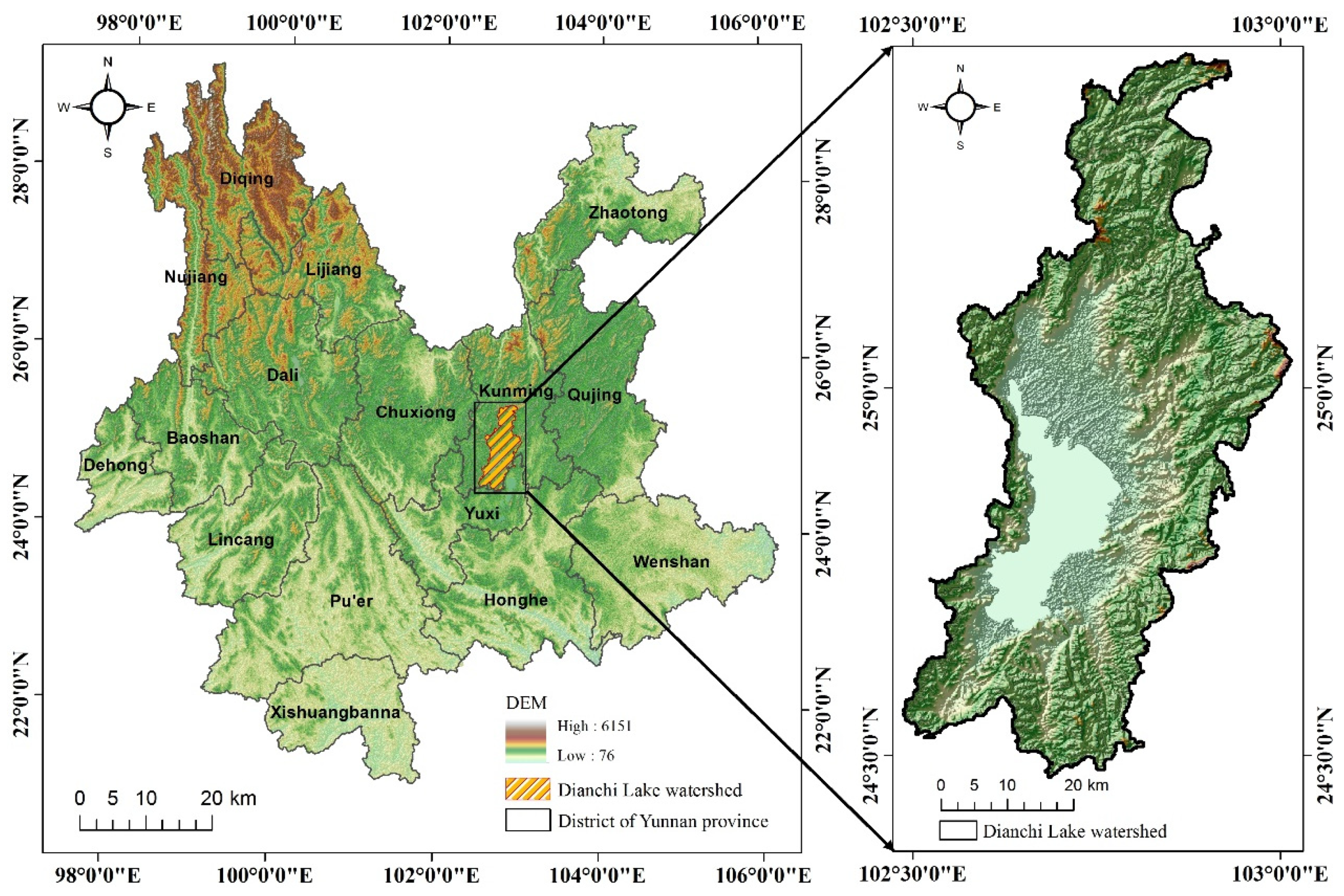
2.1. Study Area
2.2. Data and Processing
2.2.1. Data Types and Sources
2.2.2. Data Processing
2.3. Methods
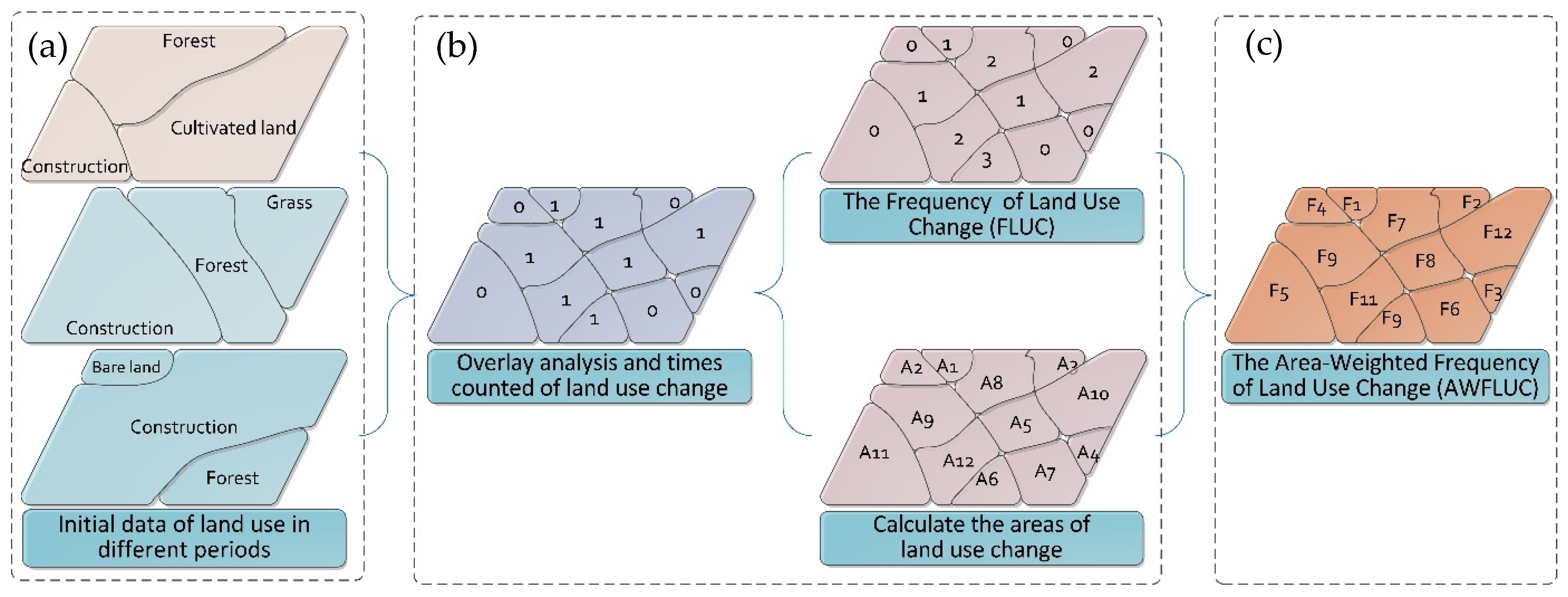
2.3.1. The Frequency of Change and Its Measurement
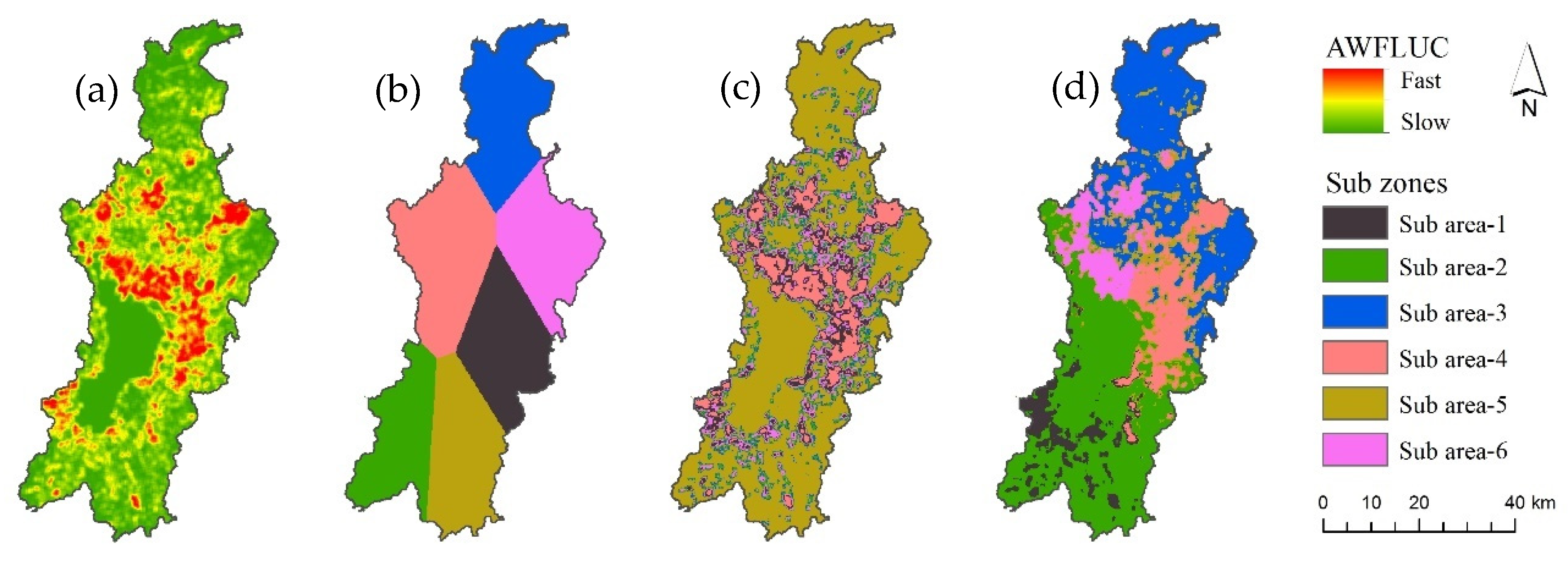
2.3.2. Cellular Space Partition Based on Dual-Constrained Spatial Clustering
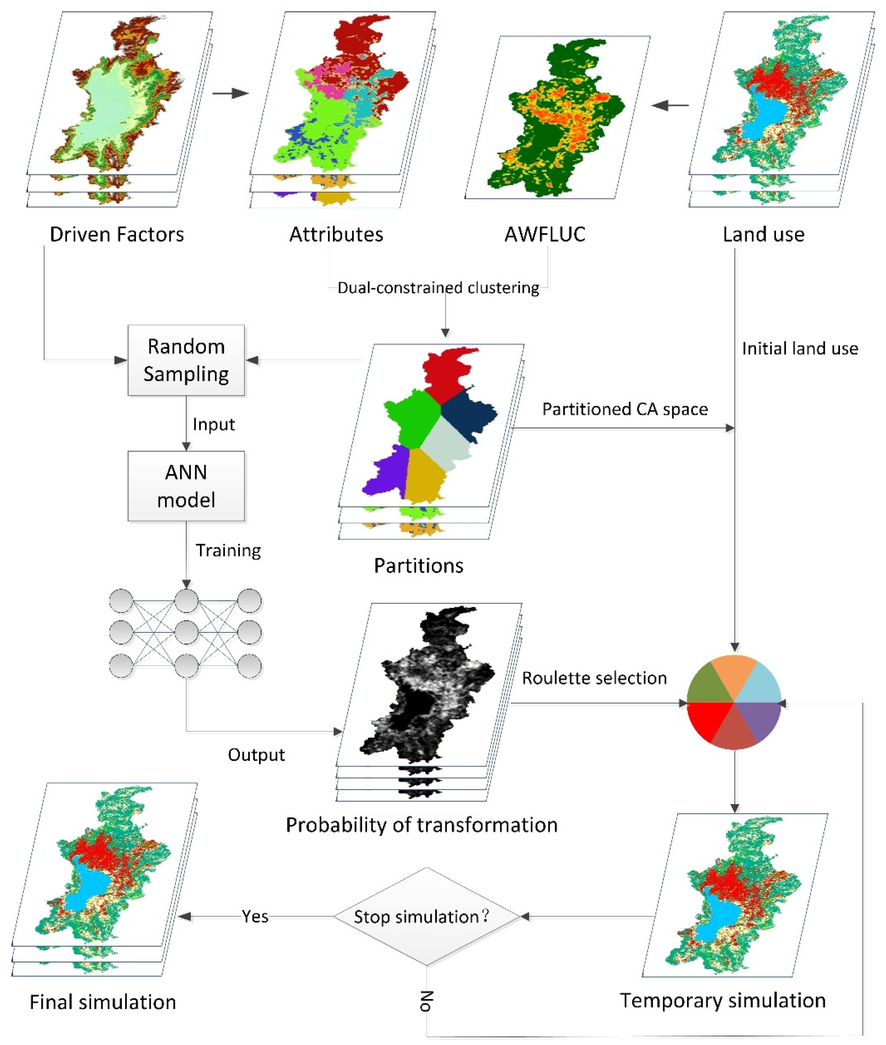
2.3.3. ANN–CA Model Construction Method of Land-Use Change
3. Results
3.1. Cellular Space Partition Results
3.2. Cellular Conversion Rules Acquisition Based on ANN
3.3. Land-Use Dynamic Simulation Results and Accuracy Test
3.4. Land-Use Dynamic Simulation Results and Accuracy Test
4. Discussion
5. Conclusions and Further Work
Author Contributions
Funding
Acknowledgments
Conflicts of Interest
Explanation of Abbreviation
| LUCC | Land-use and Land Cover Change |
| CA | Cellular Automata |
| LR | Logistic Regression |
| MC | Markov Chain |
| AI | Artificial Intelligence |
| SVM | Support Vector Machine |
| ACO | Ant Colony Algorithm |
| GA | Genetic Algorithm |
| NN | Neural Network |
| ANN | Artificial Neural Network |
| FLUC | The Frequency of Land-use Change |
| AWFLUC | The Area-Weighted Frequency of Land-use Changes |
| GDP | Gross Domestic Product |
| Model I | Non-partitioned CA model |
| Model II | Ordinary partitioned CA model (without considering AWFLUC) |
| Model III | AWFLUC-constrained partitioned CA model |
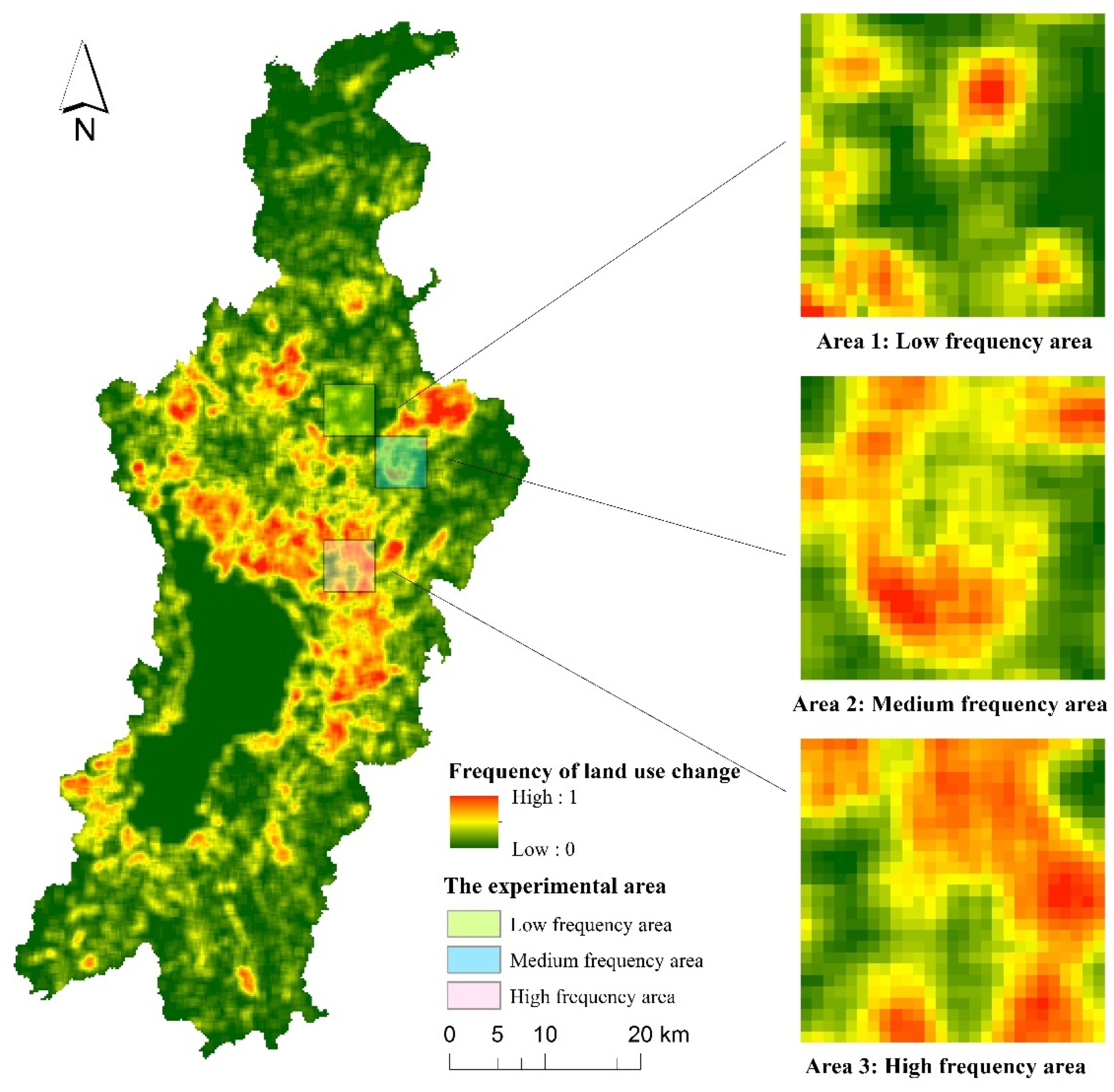
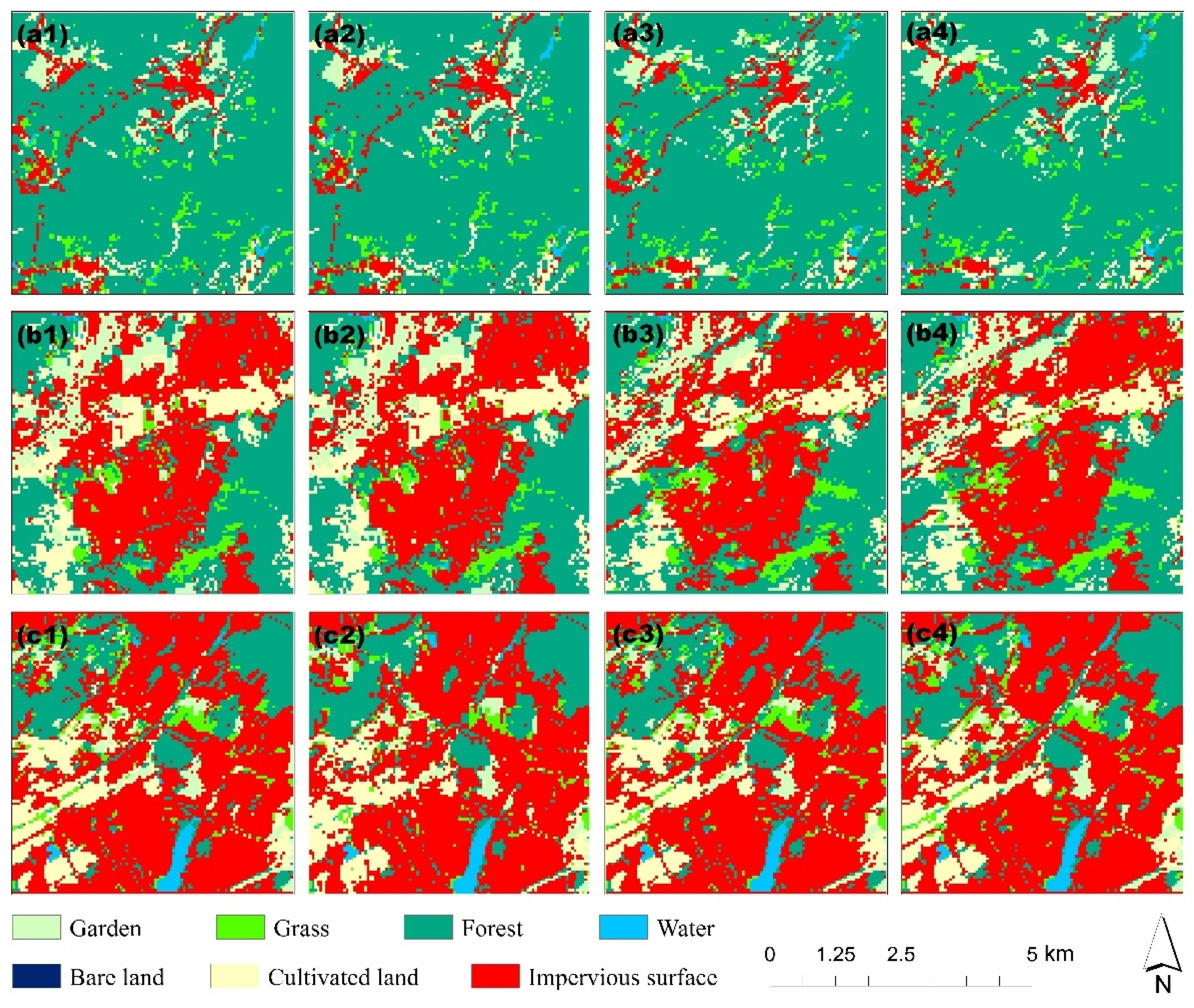
| Area 1 | Low-frequency area of land-use change |
| Area 2 | Medium-frequency area of land-use change |
| Area 3 | High-frequency area of land-use change |
| OA | Overall Accuracy |
| K | Kappa coefficient |
| AAUD | Analysis of accuracy ups and downs |
References
- Meyer, W.B.; Turner, B.L., II. Human population growth and global land-use/land-cover change. Annu. Rev. Ecol. Syst. 1992, 23, 39–61. [Google Scholar] [CrossRef]
- Verburg, P.H.; Schot, P.P.; Dijst, M.J.; Veldkamp, A. Land use change modelling: Current practice and research priorities. Geojournal 2004, 61, 309–324. [Google Scholar] [CrossRef]
- Paegelow, M.; Olmedo, M.T.C.; Mas, J.-F.; Houet, T.; Pontius, R.G., Jr. Land change modelling: Moving beyond projections. Int. J. Geogr. Inf. Sci. 2013, 27, 1691–1695. [Google Scholar] [CrossRef] [Green Version]
- Li, X.; Liu, X. Case-based Cellular Automaton for Simulating Urban Development in a Large Complex Region. Acta Geogr. Sin. 2007, 62, 1097–1109, (In Chinese with English Abstract). [Google Scholar]
- Wu, D.; Wang, R.; Gao, S.; Ding, W.; Wang, W.; Ge, X.; Liu, J. Simulation and scenario analysis of arable land dynamics in Yellow River Delta. Trans. CSAE 2010, 26, 285–290, (In Chinese with English Abstract). [Google Scholar] [CrossRef]
- Liu, X.; Liang, X.; Li, X.; Xu, X.; Pei, F.; Ou, J.; Chen, Y.; Li, S.; Wang, S. A future land use simulation model (FLUS) for simulating multiple land use scenarios by coupling human and natural effects. Landsc. Urban Plan. 2017, 168, 94–116. [Google Scholar] [CrossRef]
- Zhou, C.; Ou, Y.; Ma, T.; QIN, B. Theoretical Perspectives of CA-based Geographical System Modeling. Prog. Geogr. 2009, 28, 833–838, (In Chinese with English Abstract). [Google Scholar]
- White, R.; Engelen, G. Cellular Automata and Fractal Urban Form: A Cellular Modelling Approach to the Evolution of Urban Land-Use Patterns. Environ. Plan. A Econ. Space 1993, 25, 1175–1199. [Google Scholar] [CrossRef] [Green Version]
- Mustafa, A.; Rienow, A.; Saadi, I.; Cools, M.; Teller, J. Comparing support vector machines with logistic regression for calibrating cellular automata land use change models. Eur. J. Remote. Sens. 2018, 51, 391–401. [Google Scholar] [CrossRef]
- Lopez, S. Modeling Agricultural Change through Logistic Regression and Cellular Automata: A Case Study on Shifting Cultivation. J. Geogr. Inf. Syst. 2014, 6, 220–235. [Google Scholar] [CrossRef] [Green Version]
- Mitsova, D.; Shuster, W.; Wang, X. A cellular automata model of land cover change to integrate urban growth with open space conservation. Landsc. Urban Plan. 2011, 99, 141–153. [Google Scholar] [CrossRef]
- Lavalle, M.C. Modelling dynamic spatial processes: Simulation of urban future scenarios through cellular automata. Landsc. Urban Plan. 2003, 64, 145–160. [Google Scholar]
- Rienow, A.; Goetzke, R. Supporting SLEUTH – Enhancing a cellular automaton with support vector machines for urban growth modeling. Comput. Environ. Urban Syst. 2015, 49, 66–81. [Google Scholar] [CrossRef]
- Rienow, A.; Stenger, D.; Menz, G. Sprawling cities and shrinking regions – forecasting urban growth in the Ruhr for 2025 by coupling cells and agents. Erdkunde 2014, 68, 85–107. [Google Scholar] [CrossRef]
- Li, X.; Lao, C.; Liu, X.; Chen, Y. Coupling urban cellular automata with ant colony optimization for zoning protected natural areas under a changing landscape. Int. J. Geogr. Inf. Sci. 2011, 25, 575–593. [Google Scholar] [CrossRef]
- QuanLi, X.; Kun, Y.; Guilin, W.; Yulian, Y. Agent-based modeling and simulations of land-use and land-cover change according to ant colony optimization: A case study of the Erhai Lake Basin, China. Nat. Hazards 2014, 75, 95–118. [Google Scholar] [CrossRef]
- Shafizadeh-Moghadam, H.; Tayyebi, A.; Ahmadlou, M.; Delavar, M.R.; Hasanlou, M. Integration of genetic algorithm and multiple kernel support vector regression for modeling urban growth. Comput. Environ. Urban Syst. 2017, 65, 28–40. [Google Scholar] [CrossRef]
- Tayyebi, A.; Pijanowski, B.C. Modeling multiple land use changes using ANN, CART and MARS: Comparing tradeoffs in goodness of fit and explanatory power of data mining tools. Int. J. Appl. Earth Obs. Geoinf. 2014, 28, 102–116. [Google Scholar] [CrossRef]
- Omrani, H.; Tayyebi, A.; Pijanowski, B. Integrating the Multi-Label Land Use Concept and Cellular Automata with the ANN-based Land Transformation Model. GISci. Remote Sens. 2017, 54, 283–304. [Google Scholar] [CrossRef] [Green Version]
- Shafizadeh-Moghadam, H.; Asghari, A.; Tayyebi, A.; Taleai, M. Coupling machine learning, tree-based and statistical models with cellular automata to simulate urban growth. Comput. Environ. Urban Syst. 2017, 64, 297–308. [Google Scholar] [CrossRef]
- Yeh, G.O.; Li, X. Simulation of Development Alternatives Using Neural Networks, Cellular Automata, and GIS for Urban Planning. Photogramm. Eng. Remote Sens. 2003, 69, 1043–1052. [Google Scholar] [CrossRef] [Green Version]
- Aschenwald, J.; Fink, S.; Tappeiner, G. Brave new modeling: Cellular automata and artificial neural networks for mastering complexity in economics. Complexity 2010, 7, 39–47. [Google Scholar] [CrossRef]
- Li, X.; Yeh, G.O. Neural-network-based cellular automata for simulating multiple land use changes using GIS. Int. J. Geogr. Inf. Syst. 2002, 16, 323–343. [Google Scholar] [CrossRef]
- Li, X.; Yeh, A. Cellular automata for simulating complex landuse systems using neural networks. Geogr. Res. 2005, 24, 19–27, (In Chinese with English Abstract). [Google Scholar]
- Jantz, C.A.; Goetz, S.J. Analysis of scale dependencies in an urban land-use-change model. Int. J. Geogr. Inf. Sci. 2005, 19, 217–241. [Google Scholar] [CrossRef]
- Şalap-Ayça, S.; Jankowski, P.; Clarke, K.C.; Kyriakidis, P.C.; Nara, A. A meta-modeling approach for spatio-temporal uncertainty and sensitivity analysis: An application for a cellular automata-based Urban growth and land-use change model. Int. J. Geogr. Inf. Sci. 2017, 32, 637–662. [Google Scholar] [CrossRef]
- Kim, J.H. Spatiotemporal scale dependency and other sensitivities in dynamic land-use change simulations. Int. J. Geogr. Inf. Sci. 2013, 27, 1782–1803. [Google Scholar] [CrossRef] [Green Version]
- Wang, J.; Xu, C. Geodetector: Principle and prospective. Acta Geogr. Sin. 2017, 72, 116–134, (In Chinese with English Abstract). [Google Scholar] [CrossRef]
- Ke, X.; Bian, F. A Partitioned & Asynchronous CA Based on Spatial Data Mining. J. Image Graph. 2010, 15, 921–930, (In Chinese with English Abstract). [Google Scholar]
- Ke, X.; Deng, X.; Liu, C. Interregional Farmland Layout Optimization Model Based on the Partition Asynchronous Cellular Automata: A Case Study of the Wuhan City Circle. Prog. Geogr. 2010, 29, 1442–1450, (In Chinese with English Abstract). [Google Scholar]
- Yang, Q. Dynamic Transition Rules for Geographical Cellular Automata. Acta Sci. Nat. Univ. Sunyatseni 2008, 47, 122–127, (In Chinese with English Abstract). [Google Scholar]
- Ke, X.; Qi, L.; Zeng, C. A partitioned and asynchronous cellular automata model for urban growth simulation. Int. J. Geogr. Inf. Sci. 2015, 30, 637–659. [Google Scholar] [CrossRef]
- Zhu, H.; Li, X. Discussion on the Index Method of Regional Land Use Change. Acta Geogr. Sin. 2003, 58, 643–650. [Google Scholar] [CrossRef]
- Jain, A.K. Data clustering: 50 years beyond K-means. Pattern Recognit. Lett. 2010, 31, 651–666. [Google Scholar] [CrossRef]
- Jiao, L.; Liu, Y.; Ren, Z. Spatial Points Clustering Based on Self-organizing Neural Networks and Its Application. Geomat. Inf. Sci. Wuhan Univ. 2008, 33, 168–171, (In Chinese with English Abstract). [Google Scholar]
- Yang, J.; Shi, F.; Sun, Y.; Zhu, J. A Cellular Automata Model Constrained by Spatiotemporal Heterogeneity of the Urban Development Strategy for Simulating Land-use Change: A Case Study in Nanjing City, China. Sustainability 2019, 11, 4012. [Google Scholar] [CrossRef] [Green Version]


| Data | Data Source or Parameters | |||
|---|---|---|---|---|
| Remote sensing images | Year | Satellite and sensor | Stripe | Resolution |
| 2006 | Landsat-5 TM | 129/42, 129/43 | 30 m | |
| 2009 | Landsat-5 TM | 129/42, 129/43 | 30 m | |
| 2013 | Landsat-8 OLI/TIRS | 129/43 | 15 m | |
| 2016 | Landsat-8 OLI/TIRS | 129/43 | 15 m | |
| DEM | Year: 2016 | Source: USGS | Resolution: 30 m | |
| Railway | Year: 2006, 2009, 2013, 2016 | Source: Geospatial data cloud and OpenStreetMap | Scale: 1:250,000 | |
| Road | Year: 2006, 2009, 2013, 2016 | Scale: 1:250,000 | ||
| River | Year: 2006, 2009,2013, 2016 | Scale: 1:250,000 | ||
| Lake | Year: 2006, 2009, 2013, 2016 | Scale: 1:250,000 | ||
| Population | Year: 2006, 2009, 2013, 2016 | Source: Yunnan Provincial Statistics Bureau | Scale: 1:250,000 | |
| GDP | Year: 2006, 2009, 2013, 2016 | Scale: 1:250,000 | ||
| Data Category | Acquired Method | Range |
|---|---|---|
| 1. Land-use data | ||
| Year of 2006, 2009, 2013, 2016 | Extraction of Remote-sensing images | 1–7 |
| 2. The area-weighted frequency of land-use change (AWFLUC) | ||
| AWFLUC from 2006 to 2016 | Overlay analysis | 0–1 |
| 2. Spatial distance variables | ||
| Distance to road (X1) | Distance analysis | 0–1 |
| Distance to railway (X2) | 0–1 | |
| Distance to river (X3) | 0–1 | |
| Distance to lake (X4) | 0–1 | |
| 3. Land-use neighborhoods | ||
| Neighborhoods of impervious surface (X5) | Neighborhood analysis | 0–1 |
| Neighborhoods of cultivated land (X6) | 0–1 | |
| Neighborhoods of water (X7) | 0–1 | |
| Neighborhoods of grass land (X8) | 0–1 | |
| Neighborhoods of forestry land (X9) | 0–1 | |
| Neighborhoods of bear land (X10) | 0–1 | |
| Neighborhoods of garden land (X11) | 0–1 | |
| 4. Natural environmental variables | ||
| Slope (X12) | Surface analysis | 0–1 |
| Aspect (X13) | 0–1 | |
| Elevation (X14) | 0–1 | |
| 5. Socio-economic variables | ||
| Density of population (X15) GDP (X16) | the statistical yearbook of Yunnan province | 0–1 |
| Index | Loss Rate | |||
|---|---|---|---|---|
| Model | 2006–2009 | 2009–2013 | 2013–2016 | |
| Mode I | 0.39162 | 0.37613 | 0.34464 | |
| Model II | 0.33429 | 0.30922 | 0.27666 | |
| Model III | 0.33422 | 0.30890 | 0.28092 | |
| Accuracy Index | Model I | Model II | Model III | AAUD | |||||||||
|---|---|---|---|---|---|---|---|---|---|---|---|---|---|
| I vs. II | II vs. III | I vs. III | |||||||||||
| Period (Year) | OA | K | OA | K | OA | K | OA | K | OA | K | OA | K | |
| 2006–2009 | 0.8301 | 0.7716 | 0.8606 | 0.8133 | 0.8833 | 0.8448 | 3.68% | 5.41% | 2.64% | 3.87% | 14.48% | 9.49% | |
| 2009–2013 | 0.8477 | 0.7959 | 0.8687 | 0.8133 | 0.9007 | 0.8680 | 2.48% | 2.19% | 3.68% | 6.72% | 13.17% | 9.05% | |
| 2013–2016 | 0.8616 | 0.8151 | 0.8952 | 0.8602 | 0.9187 | 0.8920 | 3.90% | 5.54% | 2.63% | 3.69% | 12.72% | 9.44% | |
| Model I | Model II | Model III | AAUD | ||||||||||
|---|---|---|---|---|---|---|---|---|---|---|---|---|---|
| I vs. II | II vs. III | I vs. III | |||||||||||
| OA | K | OA | K | OA | K | OA | K | OA | K | OA | K | ||
| Area 1 | 0.9041 | 0.885 | 0.9198 | 0.9038 | 0.9346 | 0.9215 | 1.74% | 2.12% | 1.61% | 1.96% | 5.60% | 4.12% | |
| Area 2 | 0.8296 | 0.7956 | 0.9007 | 0.8809 | 0.9031 | 0.8837 | 8.57% | 10.72% | 0.27% | 0.32% | 13.51% | 11.07% | |
| Area 3 | 0.8891 | 0.867 | 0.9047 | 0.8857 | 0.9319 | 0.9183 | 1.75% | 2.16% | 3.01% | 3.68% | 7.49% | 5.92% | |
| AAUD | 1 to 2 | −6.69% | −8.24% | −0.44% | −0.54% | −3.09% | −3.77% | ||||||
| 1 to 3 | −1.66% | −2.03% | −1.64% | −2.00% | −0.29% | −0.35% | |||||||
| 2 to 3 | 7.17% | 8.97% | 0.44% | 0.54% | 3.19% | 3.92% | |||||||
Publisher’s Note: MDPI stays neutral with regard to jurisdictional claims in published maps and institutional affiliations. |
© 2021 by the authors. Licensee MDPI, Basel, Switzerland. This article is an open access article distributed under the terms and conditions of the Creative Commons Attribution (CC BY) license (https://creativecommons.org/licenses/by/4.0/).
Share and Cite
Xu, Q.; Wang, Q.; Liu, J.; Liang, H. Simulation of Land-Use Changes Using the Partitioned ANN-CA Model and Considering the Influence of Land-Use Change Frequency. ISPRS Int. J. Geo-Inf. 2021, 10, 346. https://0-doi-org.brum.beds.ac.uk/10.3390/ijgi10050346
Xu Q, Wang Q, Liu J, Liang H. Simulation of Land-Use Changes Using the Partitioned ANN-CA Model and Considering the Influence of Land-Use Change Frequency. ISPRS International Journal of Geo-Information. 2021; 10(5):346. https://0-doi-org.brum.beds.ac.uk/10.3390/ijgi10050346
Chicago/Turabian StyleXu, Quanli, Qing Wang, Jing Liu, and Hong Liang. 2021. "Simulation of Land-Use Changes Using the Partitioned ANN-CA Model and Considering the Influence of Land-Use Change Frequency" ISPRS International Journal of Geo-Information 10, no. 5: 346. https://0-doi-org.brum.beds.ac.uk/10.3390/ijgi10050346