Article

Do Mobile Phone Data Provide a Better Denominator in Crime Rates and Improve Spatiotemporal Predictions of Crime?

1
Department of Criminology, Criminal Law and Social Law, Ghent University, 9000 Ghent, Belgium
2
Department of Geography, Ghent University, 9000 Ghent, Belgium
3
Department of Marketing, Innovation and Organization-Data Analytics, Ghent University, 9000 Ghent, Belgium
4
Faculty of Social Sciences, University of Antwerp, 2000 Antwerp, Belgium
*
Author to whom correspondence should be addressed.
ISPRS Int. J. Geo-Inf. 2021, 10(6), 369; https://0-doi-org.brum.beds.ac.uk/10.3390/ijgi10060369
Submission received: 6 April 2021 / Revised: 25 May 2021 / Accepted: 27 May 2021 / Published: 31 May 2021
(This article belongs to the Special Issue Geographic Crime Analysis)

Abstract

:
This article assesses whether ambient population is a more suitable population-at-risk measure for crime types with mobile targets than residential population for the purpose of intelligence-led policing applications. Specifically, the potential use of ambient population as a crime rate denominator and predictor for predictive policing models is evaluated, using mobile phone data (with a total of 9,397,473 data points) as a proxy. The results show that ambient population correlates more strongly with crime than residential population. Crime rates based on ambient population designate different problem areas than crime rates based on residential population. The prediction performance of predictive policing models can be improved by using ambient population instead of residential population. These findings support that ambient population is a more suitable population-at-risk measure, as it better reflects the underlying dynamics in spatiotemporal crime trends. Its use has therefore much as-of-yet unused potential not only for criminal research and theory testing, but also for intelligence-led policy and practice.

1. Introduction

In many fields, decision-making processes are increasingly based on intelligence gained from big data, complex datasets containing large amounts of data, from which new information can be extracted. Although the use of big data is relatively new in criminology, there are a lot of opportunities to increase our knowledge and improve data-based applications by leveraging big data [1,2]. This is particularly true for intelligence-led policing, with its focus on data-based, proactive policing [3]. Within the scope of intelligence-led policing, crime data analysis is used to objectively inform policy, policing strategies, and tactical operations in order to reduce and prevent crime [4]. In that respect, the use of big data offers an opportunity to improve the analysis and prediction of spatiotemporal concentrations of crime.
It is empirically well-established within environmental criminology that crime patterns show significant spatiotemporal variability, with crime concentrations at specific times (i.e., burning times) and specific places (i.e., hotspots) [5,6,7]. The areas and times under investigation differ in several ways, such as magnitude, population characteristics, and number of visitors (e.g., work-related or tourists). To take those differences into account, crime rates or indexes are frequently used within criminological research. A crime rate is “a statistic often used to represent the risk of criminal events [and that] help[s] to reveal clusters of crime in space and/or time based on an underlying population at risk” [8] (p. 112). They allow for a more valid comparison of different spatiotemporal units (e.g., small city vs. metropolitan city), control for specific characteristics of the units of analysis, and reflect the population at risk to draw meaningful conclusions regarding spatiotemporal patterns of crime and its predictors. A frequently used denominator is residential population. It is a relatively easily obtainable variable via official instances (and often also via open data platforms) and has been shown to have a strong correlation with crime in general. For the same reasons, residential population is also a commonly used (control) variable in statistical models used to predict or explain spatiotemporal patterns in crime.
However, using residential population in crime analysis has one main problem: as it is a static measure, it does not take into account the spatiotemporal mobility of perpetrators, victims, and guardians [9,10]. This is reflected in, for example, the effect of day and night cycles, holidays, weekends, and commuting hours [11] (p. 346). Similarly, uninhabited areas with a lot of comings and goings (e.g., parks or business areas) can definitely generate or attract crime [12]. As a consequence, the residential population is not always, specifically for crime types with mobile targets and/or perpetrators, a valid representation of the actual population or targets at risk for a given place and time.
A possible alternative to residential population which could better reflect this spatiotemporal mobility and therefore the actual population at risk, is ‘ambient population’. The ambient population is the number of people present in a given area at a given time [13] and is typically estimated using big data such as mobile phone data. The first efforts to estimate the ambient population date from the mid-2000s, but, mainly due to the ubiquity of smartphones and social media, those efforts have increased recently, since circa 2014. Crowd and footfall dynamics have been related to crime and the findings show that these have a substantial impact on crime rates from the idea that “daily nonresidential activities distribute crime unevenly over space, beyond residential effects” [14] (p. 1). Using ambient population instead of residential population could therefore result in a more valid measure of the population-at-risk and consequently improve applications depending on this measure, such as crime rates/indexes and statistical models of spatiotemporal crime patterns, such as those used in predictive policing.
In this study, we apply mobile phone data as a proxy of ambient population in two intelligence-led policing applications: crime rate analysis and crime risk prediction. In both cases, the performance of ambient population is compared with that of residential population. Our main research question (RQ) and sub-questions are as follows:
RQ: To what extent is there a stronger relationship between crime and a population measure when using ambient population compared to the residential population?
  • To what extent do crime rates differ when calculated based on the ambient population compared to the residential population?
  • From the two population-at-risk measures (ambient population and residential population), which one is a better predictor for the predictive analysis of crime events?
We hypothesize that, for crime types with a mobile target, the ambient population provides a more accurate denominator in calculating crime rates and improves spatiotemporal crime predictions.

2. Background

In what follows, we will elaborate on relevant prior research. First, we will briefly describe two outstanding problems related to using residential or ambient population in crime analysis. Second, we will outline the developments over time, distinguishing between different ‘generations’ of data sources used to estimate ambient population. Third, we will succinctly summarize the studies that have used mobile phone data to assess the ambient population in relation to crime.

2.1. Residential Versus Ambient Population: Related Challenges

As stated earlier, it is important to consider spatiotemporal variability in the analysis of crime. This raises two inter-related challenges: on the one hand, the choice of (or the availability of data on) the most appropriate (valid) population-at-risk measure and on the other hand, the choice of (or availability of data on) the most appropriate (spatiotemporal) units of analysis.

2.1.1. Determining the Most Appropriate Population-at-Risk Measure

The population-at-risk is an important measure in the calculation of crime rates and as a controlling variable for spatiotemporal crime models. Boggs [9] gives substance to this proposition stating that crime rate denominators should be related to the potential crime targets, or as Skogan (1976, cited in [15]) formulated it, “potential opportunities for victimization” (p. 216). In terms of the routine activity theory [16], the population-at-risk measure should be related to the suitable targets of the specific type of crime. In the case of crime rates for car theft, for example, the number of stolen cars is the numerator and the number of all the cars present in a particular area should be, ideally, the denominator in order for the measure to reflect the actual risk. However, data on these populations of interest are not always available and hence a proxy is often used to get as close as possible (e.g., number of parking places to measure the number of cars present in a particular area).
The use of the residential population contains the implicit assumption that this is a suitable, general representation of the population-at-risk, or at least a close equivalent to the actual population-at-risk. However, prior research has found that it is important to control for targets at-risk and differences in opportunity structures [17], and, hence, to determine the most appropriate population-at-risk measures for specific crime types [9], because the use of a single measure may hide significant variances or mask more specific crime patterns for each and every crime type.
Using residential population can therefore be problematic as for certain crime types, (1) individuals are not at the highest risk of victimization when being at home, but when they are, for example, commuting (e.g., [18]); (2) although there is a general tendency from offenders to commit crime within their awareness spaces, not all crimes are committed near their home, but also away from their (current) homes, for example in the case of robbery (e.g., [19,20]); and (3) mobile targets (such as cars or people) move through space and time, which means that their risk of victimization varies over space and time; in other words, the distinction between mobile and immobile targets [21] is essential in terms of the risk of victimization.

2.1.2. Determining the Most Appropriate Unit of Analysis

Geographical research, not limited to criminology, has paid a lot of attention to the modifiable areal unit problem (MAUP) [22,23,24,25]. MAUP involves the problem of (choices in) data aggregation at a geographical level and the resulting determination of which events are included in that area and which are not. It has two dimensions: on the one hand, the issue concerning which zoning system (shape or polygon form) of areal units is the most appropriate in a specific study (also known as the ‘zonation effect’) and on the other hand, the issue due to spatial (dis)aggregation or changes in the spatial resolution of the data (also known as the ‘scale effect’; [24]). MAUP has received considerable attention in ecological research within criminology (e.g., [6,26]).
Studies within environmental criminology show that crime is concentrated at micro places (e.g., [6,27]), even to such an extent that Weisburd postulates a law of crime concentration at places that states that “for a defined measure of crime at a specific microgeographic unit, the concentration of crime will fall within a narrow bandwidth of percentages for a defined cumulative proportion of crime” [28] (p. 138). Although uniform standards for reporting and summarizing crime concentrations are not yet established [29] and this ‘law’ concerns a mere descriptive-empirical observation that raises more questions than answers [30], Weisburd and colleagues state that 50% of crime is concentrated at approximately 4% of the micro places and 25% of crime is concentrated at less than 1.5% of the micro places [31]. Therefore, particular interest should be given to the examination of crime trends at small scales, such as addresses, fine-grained grid cells, street segments, or clusters of these [6,32]. This ‘criminology of place’ distinguishes itself from earlier schools of thought with an interest in geographic aspects of crime (prevention) by focusing on units of analysis that are smaller than the census tracts or census block groups that are generally used to define neighborhoods [7].
Largely ignored, however, is its temporal counterpart, the modifiable temporal unit problem (MTUP) [33,34]. MTUP refers, analogous with MAUP, to the problem of (choices in) data aggregation, but on the temporal level. This also determines which events are included in a particular time frame and which are not. MTUP has three dimensions: the first refers to temporal aggregation or the unit of time observation (‘scale effect’, e.g., minute, hour, or day); the second refers to the manner in which the temporal units are divided (‘segmentation effect’, e.g., starting a week on Sunday or Monday), and the third refers to the adjustments to the temporal extent of a time series (‘boundary effect’, i.e., the arbitrary start and end points of a time series) [33]. Although this ignorance is theoretically difficult to justify [35], it is explainable given the former unavailability of temporal fine-grained data at that time. Currently, these data constraints—theoretically—no longer apply, since new and emerging data sources (or big data) hold the promise of “a data deluge – of rich, detailed, interrelated, timely and low-cost data – that can provide much more sophisticated, wider scale, finer grained understandings of societies and the world we live in.” [36] (p. 263). These new and emerging data sources, such as GPS data and mobile phone data, provide large opportunities for research in environmental criminology [2,15].
Since both the spatial and temporal dimension are important to capture the setting in which rule-breaking behavior takes places, it is more appropriate to assess the ‘unit problems’ of (the convergence of) both dimensions. This results in the ‘modifiable spatio-temporal unit problem’ (MSTUP) [37]. Both dimensions vary with scale, depending on the degree of both spatial and temporal heterogeneity. Meentemeyer states that “[i]n essence the scales need to match the heterogeneity; i.e., the phenomenon dictates the scale” [38] (p. 171).
The MSTUP in particular is a persistent challenge that lies ahead in spatiotemporal analyses of crime. Prior research shows that not only crime is concentrated at micro places and small units of time (e.g., [39,40]), but also that a varying spatiotemporal resolution has implications for crime prediction [41]. Making the scale too small comes with its own problems, the most important being data availability and data sparsity (i.e., a disproportionately high number of zeros). This is generally caused by the low frequency at a fine-grained spatiotemporal scale and requires at best correction mechanisms or at worst a higher aggregation level to be able to draw meaningful conclusions [41,42,43].

2.2. Developments in Measuring the Ambient Population

In the past, scholars have used various methods to estimate the ambient population. We can distinguish different ‘generations’ of data sources used to estimate the ambient population.
First, so-called commuter-adjusted populations estimates correct the residential population parameter with an observation- or survey-based approach to account for incoming and outgoing commuters. For example, Oberwittler [44] used public transport passenger counts as a proxy measure for non-residential population in estimating the population-at-risk. Later, Stults and Hasbrouck [11] studied between-city variance in crime rates, considering commuter inflows in the denominator of the crime rate. Felson and Boivin [14] studied within-city variance in crime rates, considering survey-based visitor inflow data to measure population shifts and, hence, estimate the ambient population. These survey-based measures provide, however, information from a snapshot in time.
Second, (ancillary) administrative data and remote sensing datasets (e.g., LandScan Global Population Database) have been used to estimate the ambient population as an alternative for the residential population (e.g., [13,14,15,16,17,18,19,20,21,22,23,24,25,26,27,28,29,30,31,32,33,34,35,36,37,38,39,40,41,42,43,44,45]). The LandScan algorithm uses spatial data and imagery analysis to disaggregate census data within an administrative boundary [46]. The LandScan database contains an average population count for grid cells of approximately 1 km × 1 km and averaged over 24 hours. In the absence of alternatives, this data source has provided useful insights. However, these spatial and, mainly, temporal scales are still too coarse to be meaningful, as spatial and temporal fluctuations are not well-displayed.
Third, user-generated content, such as data from social network sites, has been used as a proxy indicator for the ambient population. Malleson and Andresen [8,47,48] and Hipp et al. [49] used Twitter data as an estimate of the ambient population. They used all geo-located tweets in a specific area as a proxy measure of the ambient population. Kounadi et al. [32] used a Twitter dataset as an ancillary dataset to extract control points to redistribute a population dataset with coarse resolutions among micro places. Another dataset originating from social network sites that is empirically used to calculate crime rates innovatively is a FourSquare dataset. Kadar et al. [50] used both venues and check-ins from FourSquare in the constitution of indicators for the ambient population. Despite the large opportunities from these user-generated data sources, like low-cost and real-time availability, these data sources have some major drawbacks. Foremost, these user-generated data have a large coverage error [51], because the population is not equally represented. This inequality is due to, on the one hand, the ‘digital divide’ [52] (i.e., the inequality in information access, which in this case is pronounced by the lower mobile phone use of specific groups, such as the elderly) and, on the other hand, the use of geo-tagged data that are needed for this application. Geo-tagged data are another subsample within the subsample of users of the social network sites [47]. Recently, scholars also employed user-generated cell tower location data to calculate a proxy measure of the ambient population [53].
Fourth, data from mobile phones have been used to estimate the ambient population. Bogomolov et al. [54] can be seen as pioneers at this point within criminology. They found that this data source significantly improves crime prediction accuracy, compared to “traditional, rich – yet expensive to collect – statistical data about a borough’s population” [54] (p. 433). We will further elaborate on this data source in the next paragraph.

2.3. Previous Studies on Crime Concentrations Using Mobile Phone Data as a Proxy for Ambient Population

Data from mobile phones provide unprecedented insights into human behavior and its dynamics. In this data-intensive era, the global adoption of mobile information and communication devices and human interaction through these mobile devices create digital footprints of people, both in space and time [55,56]. In 2018, 96% of Belgian inhabitants between 16 and 74 used a mobile phone, either a smartphone (78%) and/or a cellphone (20%) [57]. These ubiquitous mobile phones are considered a proxy measure for the ambient population [58]. However, it is noteworthy that this share is not equally distributed over the general population. For example, for people in the youngest age category (16–24 years), the share of using a mobile phone was 99%, compared to a share of 80% for people in the oldest age category (65–74 years; note that people under age 16 and above age 74 were not included in Statbel’s [57] study). For the use of a smartphone, this discrepancy was even more pronounced: respectively, 95% versus 37% [57].
Prior empirical research within environmental criminology successfully used mobile phone data as a measure of the ambient population. These prior studies have in common that they used mobile phone data to assess crowd and footfall dynamics in space and time, but the methodological approaches differed between the studies. All studies departed explicitly or implicitly from (aspects of) crime opportunity theories, mostly routine activity theory [16] and/or crime pattern theory [59]. Most of the studies focused on predicting spatiotemporal crime patterns on the one hand and/or explaining those spatiotemporal crime patterns on the other hand. More specifically, mobile phone data were of course used as a proxy measure of the ambient population, but the indicators that were included in the analyses depended on the availability of relevant breakdowns in the dataset, such as information regarding origin (i.e., estimated number of residents, workers, and visitors), gender (i.e., estimated number of males and females), and age categories (e.g., [54]), which allowed for examining the relative importance of the presence of subgroups within the ambient population. Note that Song and colleagues [60] differed in their approach, since they used mobile phone data to measure mobility of people and noted the mere presence of people in time and space. Contrary to the other studies, they sought to explain offenders’ target location choice.
Regarding the methodology used, there were several differences between the studies. To begin with, as summarized in Table 1, the studies differed considerably in the spatial and temporal scales used. Second, the analytical approaches were different. As mentioned before, some studies merely sought to predict spatiotemporal crime patterns, where others tried to (more theoretically informed) explain spatiotemporal variation in crime. Third, there was a difference in the crime types assessed. Most of the studies focused on theft from the person offences [48,60,61,62] or specific sub-types thereof: snatch-and-run offences [63]. In the study of Bogomolov et al. [54,64], a general crime measure was composed based on eleven different crime types. Traunmueller et al. [65] distinguished between street crime (e.g., antisocial behavior, drugs, robbery, and violent crime) and home crime (e.g., burglary, criminal damage, and arson, other theft, and shoplifting). Haleem et al. [66] and Lee et al. [67] used data on violent crime in their study. Table 1 provides information on several general descriptive characteristics of prior research on spatiotemporal patterning of crime with mobile phone data.
All relevant prior studies focusing on crime prediction found that introducing the ambient population measure yielded higher predictive accuracy than the residential population [54,64]. Additionally, in all relevant prior studies focusing on explaining spatiotemporal crime variation, the inclusion of the ambient population measure yielded significant results in correlation analyses [48,65,66], and the introduction of this measure in regression analyses significantly improved the models [61,62,63]. However, two important observations need to be mentioned. First, the performance of the ambient population measure seemed to vary throughout the day, which means that at specific moments of the day, other proxy measures of the ambient population performed better (e.g., taxi ridership in [61] or the workday population measure (based on a survey-based correction of the residential population dataset) in [48]). Second, it has to be noted that all conclusions of prior studies have to be seen in the light of their own limitations and in the light of the crime types studied.
It is noteworthy that mobile phone data can be and are approached differently (see column ‘Data type’ in Table 1). One can use the level of activity, so every action (e.g., sending an SMS or making a call) is present in the dataset as an individual case. One can also use the number of unique devices, so every device is (after at least one action) counted only once. In addition, one can choose between the types of signaling data, for example, one can include any type of action, call data records, or Internet activity. Finally, a major drawback of most of the aforementioned studies is some spatial and/or temporal incongruences between the data sources used. This results in a necessary aggregation of other data for compatibility reasons and, even worse, a lack of fine-grained spatiotemporal information. For example, most crime data used are only available on a monthly aggregated basis, lacking temporal variations [48,54,62,64,65], which results in a necessary aggregation of the fine-grained (mostly hourly) mobile phone data (see Table 1). Another example, from a spatial perspective, is the study of He et al. [62], where spatially fine-grained mobile phone data (grid cells of 306 by 306 meters) were aggregated to considerably larger units of analysis (Paichusuo territorities; i.e., police sub-station areas; 54.34 km2 on average).

3. Materials and Methods

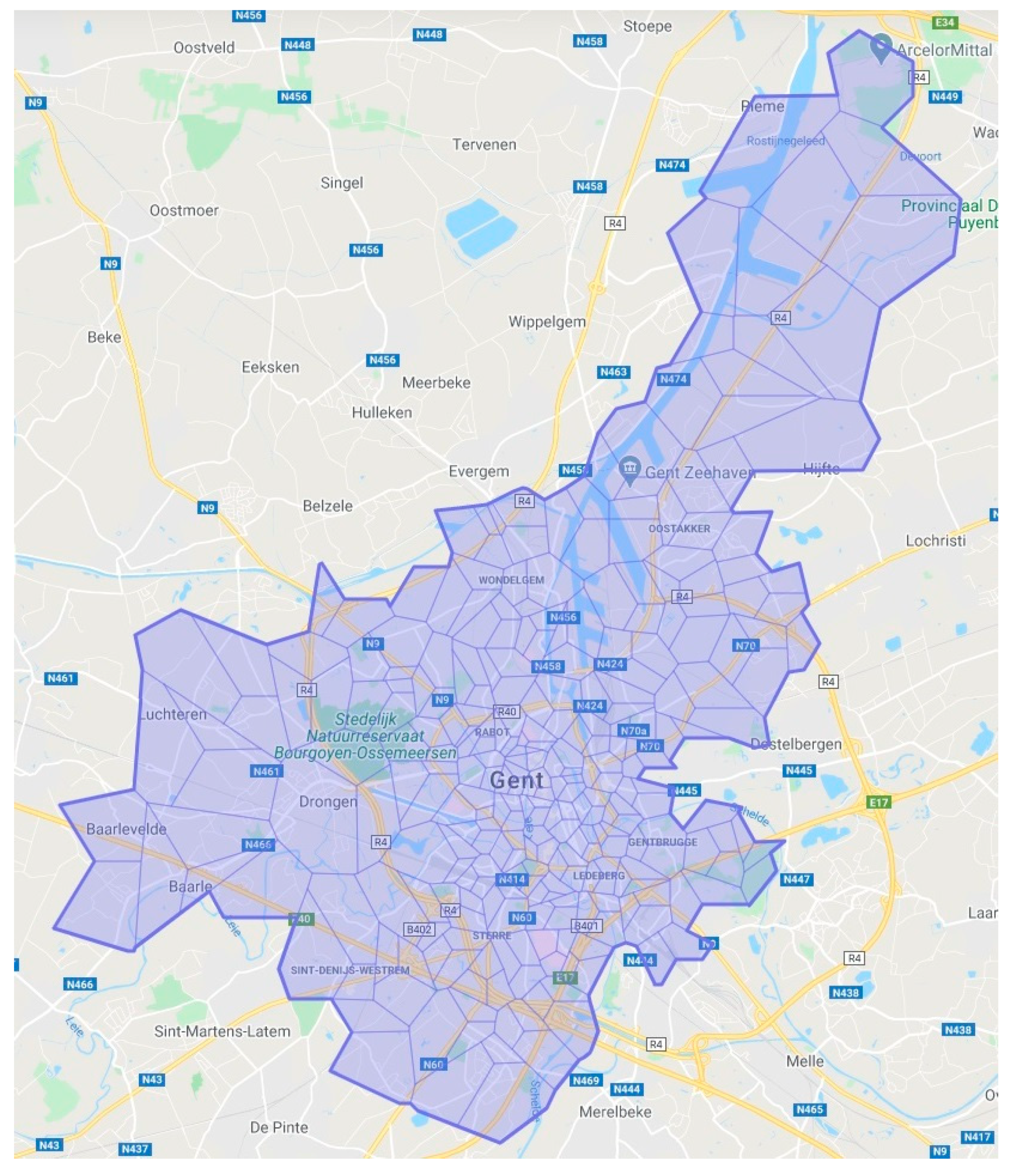
3.1. Description of the Study Area and Spatial Units of Analysis

The study area for our crime and ambient population analysis was the city of Ghent. With 261,475 inhabitants in 2018, it is the second largest city in Belgium after Antwerp.
Two spatial units of analysis were used in this study: the statistical sector level and the grid level. Statistical sectors (N = 201 for Ghent) are generally the smallest meaningful units of analysis in Belgium for which demographic and socio-economic data are systematically collected and analyzed, and are comparable to census tracts in the United States and output areas in the United Kingdom. They are based on socio-economic, morphological, and land use characteristics [68]. They are commonly used in social-ecological research and policy and practice applications (e.g., crime statistics reports). To compare the crime rates when calculated with the ambient population versus the residential population (sub-RQ1), we conducted our analysis at the statistical sector level.
Grids or street segments are most commonly used in the spatial modeling of crime. In practice, a major application of the prediction of crime events is its use by police departments to optimize patrols (the ‘predictive policing’ approach) and therefore they require small spatial units. Our intent was to test the potential of using the ambient population specifically for this purpose, relative to the residential population. Therefore, to compare ambient and residential population as predictors for the predictive analysis of crime (sub-RQ2), a raster grid with a resolution of 200 by 200 meters was used as the spatial level of analysis (N grids = 4206). Grid cells with this resolution have also previously been applied successfully in empirical criminological research (e.g., [30,41,69,70]).

3.2. Data Sources and Measurement of Key Constructs

The data used for this analysis stem from three sources: crime data collected by the Ghent Local Police Force, administrative data on the residential population collected by the City of Ghent, and data on the ambient population collected by the mobile phone operator Proximus.
The Ghent Local Police force provided crime data for three crime types from October to December 2018: aggressive theft, battery, and bicycle theft. Aggressive theft is defined as purse snatching or robbery using a weapon or threats, including attempts. Battery is defined as the intentional use of force or violence resulting in injuries, intra-familial violence is excluded. Bicycle theft is defined as simple theft of locked or unlocked bicycles in the public space, including attempts. We need to be aware that the willingness to report (from the side of citizens) and the willingness to register (from the side of the police) differs per crime type. Bicycle theft, for example, is among the most recorded crime types in Belgium and is actually the most recorded crime type in the region of Flanders [71]. However, the results from the most recent Belgian Security Monitor indicate that bicycle theft is among the crime types with the lowest citizens’ willingness to report: in the 12 months prior to the data collection, 10% of Belgian households reported being a victim of bicycle theft, but only 48.1% reported this to the police [72].
We chose these crime types to include both violent and property crime in our analysis. For each of these crime types, we received the following data for each event in the study period: the location at the address level and the exact time or time range during which the crime was assumed to have taken place based on the information given by the victim when registering the crime. If only a time range was available, the time of the crime event was assumed to have taken place at the midpoint of this range in the following analyses. After data cleaning and geocoding, our dataset contained 49 cases of aggressive theft, 293 cases of battery, and 571 cases of bicycle theft for further analysis. The crime data were geocoded by the researchers based on the official address reference database of Flanders (‘Centraal referentieadressenbestand’ or CRAB). If no full address was available (aggressive theft: 67.80% of the cases, battery: 35.06% of the cases, bicycle theft: 34.15% of the cases), a grid cell was randomly assigned from the grid cells overlapping the street. Crime events with no registered street were excluded (aggressive theft: 13.56% of the cases, battery: 1.56% of the cases, bicycle theft: 0.98% of the cases).
The crime data were then aggregated to crime counts for each crime type and for each month per statistical sector for the statistical sector analysis and to crime counts for each crime type and for each month per grid cell for the grid level analysis. Due to the high number of zero cells (more than 95%) and the low number of cells with more than one incident, the crime variable was additionally dichotomized for the grid level analysis (i.e., 0 = no incident for a given grid cell during a given period, 1 = one or more incidents happened in a given grid cell during a given period).
Data on the residential population was obtained via the City of Ghent. They provided counts of inhabitants for each 200 by 200 meter cell of the grid we provided, and their respective statistical sectors, based on the, at the time most recently (2018) available, data from the population register. Due to privacy reasons, the city masked grid cells with four or fewer (but not zero) inhabitants (6.28% of the grid cells). Those cells were shown to have four inhabitants (i.e., a count of four inhabitants means four or fewer inhabitants). Cells with zero inhabitants (48.19%) were not masked.
Finally, the ambient population was estimated using mobile phone data from Proximus as a proxy. Proximus is the largest mobile phone operator in Belgium, holding a market share of 39.10% [73]. Specifically, the mobile phone data consist of counts of individual (smart)phones (unique users) connected to the Proximus network and present in Ghent. To produce counts at a small spatial level, Proximus used a hexagonal grid (Thiessen polygons) centered by their cell phone antennas (with a total of 288 cells for the area of Ghent). The size of the individual cells depends on the population density: the higher the population density, the smaller the cells, as there are more antennas in those areas (see Figure 1).
The number of present phones was counted per hour for each cell of the grid during a period of three months for a total of 9,397,473 data points. Due to privacy reasons, Proximus excluded cells with thirty or fewer phones present (1.06% of the data points in the raw data; in the aggregated datasets used for our analysis, no cases had zero mobile population) and only allowed three months of data to be collected in total. The counts were then extrapolated to the total population proportional to the market share of Proximus in Belgium. Finally, the counts in the hexagonal grid were mapped to the rectangular 200 by 200 meter grid cells and assigned to their respective statistical sectors.

3.3. Data Analysis Methods

To investigate the relationship between crime and both the residential and ambient population in general, correlation coefficients were calculated for both the dataset with the statistical sector as the unit of analysis (which was then used for the crime rate analysis) and the dataset with the 200 by 200 meter grid cells as the unit of analysis. The correlation coefficients were calculated for each crime type and for each of the three months in the dataset to check for monthly variations. For the statistical sector dataset, the Pearson correlation coefficient was used, while for the grid dataset, the point bi-serial correlation coefficient was used due to the binary nature of the crime variable in that case. In addition, the difference between residential and ambient correlation with crime was tested using Zou’s confidence interval test of the difference between two correlations [74,75].
To investigate whether using the ambient population as the denominator of crime rate would lead to different results than using the residential population as a denominator (sub-RQ1), crime rates were calculated for each statistical sector based on residential population and ambient population. If a statistical sector had zero population, this sector was excluded, as it would not be possible to calculate a residential population crime rate. Only one sector was excluded for this reason, and for this particular sector, no crimes for any of the three crime types were registered during the study period (October to December 2018).
To investigate whether the ambient population could be a better predictor of crime than the residential population (sub-RQ2), we used predictive analysis. Specifically, we used logistic regression to build two one-variable models: one with a residential population as the predictor of the probability that a new crime event would happen in each grid cell and one with an ambient population as the predictor for the probability that a new crime event would happen in each grid cell. The available data were split into a training and a test set. The data from October to November were used as the training dataset to train the predictive model in predicting crime events. The December data was used as the test set, to evaluate the prediction performance, i.e., the crime locations (grid cells) for the month December were predicted. To compare the residential and ambient population models, both models predicted the same fixed number of crime events depending on the average monthly number of crimes.
Prediction performance was evaluated using the following measures: recall, precision, F1-score, and AIC. Recall is the proportion of incidents predicted correctly versus the total number of incidents. Precision is the proportion of correctly predicted grid cells versus the total number of grid cells predicted at risk. Ideally, a good scoring model has both a high recall and precision. To reflect this, we also included the F1-score. The F1-score is the harmonic mean of recall and precision and therefore considers both in one measure. Finally, the Akaike Information Criterion (AIC) is a measure which allows comparison of different models on the same data, taking into account both goodness-of-fit and model simplicity. It estimates the relative amount of information lost by the model: the less information loss, the better the model. The model with the lowest AIC is therefore generally the better model. The more traditionally used Receiver-Operating Characteristic (ROC) curve and its associated Area Under the Curve (AUC) measure were not used here as they can be misleading when there is moderate to severe class imbalance [76,77], as was the case here due to the relatively low crime frequency.

4. Results

4.1. Correlation Analysis

To gain more insight into the relationship between crime and population, comparing residential and ambient population with each other, we used correlation analysis. Table 2 shows the resulting correlation coefficients at the statistical sector level for each of the three crime types versus residential and ambient population for each month in the study dataset.
In all cases, the relationship between crime and population, both ambient and residential, was positive. The correlation between crime and ambient population was significant with p < 0.001 for all crime types. All three crime types also showed a stronger correlation with ambient population than with residential population. The strongest relationship was between bicycle theft and ambient population (with a correlation coefficient of 0.60 in November). The correlation differences were also significant, with the exception of aggressive theft in October and November, where no significant difference was detected. In general, the relationship between crime and population was consistent between months, with the exception of aggressive theft (especially residential population), which might be caused by the lower frequency of that crime type.
When looking at correlations at the grid level (see Table 3), ambient population similarly showed a stronger relationship with crime than residential population. The difference was less pronounced than for the analysis at the sector level, but this is likely due to the much smaller scale and the consequent data sparsity. All correlation coefficients were positive and significant. The strongest relationship was once again between bicycle theft and ambient population (with a correlation coefficient of 0.47 in October). All correlation differences were significant, confirming that ambient population had a stronger correlation with crime for all crime types.

4.2. Crime Rates Based on Residential Population Versus Ambient Population

Based on the available data, we calculated two crime rates: one with residential population as the denominator and one with ambient population as the denominator. For the majority of statistical sectors, ambient and residential population agreed with each other. However, there were several sectors where using ambient or residential population as the denominator for crime rate made a significant difference. Table 4 lists these sectors for each crime type with a large difference between ambient and residential crime rate (defined as a difference between the standardized scores >2) with their main characteristics and nearby landmarks.
For these sectors, the crime rate based on ambient population tended to highlight different areas than the crime rate based on residential population. In some cases, the ambient crime rate was higher on average than the residential crime rate (e.g., sector C72), while in some cases, it was lower (e.g., sector A46). In the latter case, the differences were largely due to the differences in size of the ambient population versus the residential population. Ambient crime rate tended to be lower in sectors with the presence of facilities with a high ambient population (e.g., train station, sports stadium, recreation area) in low-populated areas, suggesting that while crime rate might seem relatively high when looking at the residential population, it was not that high when taking into account the actual amount of people coming and going in that area. These areas can be considered crime generators, i.e., activity nodes in which daily activities take place and that pull a large number of individuals, including potential targets and offenders [12]. In the case of bicycle theft, sector A46 was a special case, as the sign was reversed for the ambient crime rate, suggesting that the ambient crime rate was lower than average for this sector, while the residential crime rate was higher than average.
More interesting are the sectors where the situation was reversed, i.e., where the ambient crime rate was higher on average. In many of these sectors, this happened despite the previously mentioned discrepancy between high ambient population and low residential population (e.g., sectors A35 and E32 in the vicinity of large train stations). These areas can be considered crime attractors, i.e., places or facilities that have a reputation for the crime opportunities being present and where offenders gravitate with the intention of committing crime [12]. This would suggest that even taking into account the actual ambient population, the crime rate is problematic in those sectors. In other sectors (e.g., sectors C72 and A542), it is not immediately clear what causes the relatively higher ambient crime rate. They might be problem areas, which would have gone unnoticed if only the residential crime rate was studied.

4.3. Predictive Analysis Using Residential Population Versus Ambient Population

Based on the data of the two preceding months (October and November 2018), we made crime event predictions for aggressive theft, battery, and bicycle theft in December 2018. As stated in the methodology section, these were one-variable models to isolate the performance of residential and ambient population specifically. Table 5 compares the resulting prediction performances of the residential population model and the ambient population model.
Note that for aggressive theft, only 20 crime events were registered. The residential population model was only able to predict one incident. The ambient population, on the other hand, performed better by predicting 25.00% (5 crime events) with a precision of 8.00%, which means that of the 20 predicted grid cells at high risk, two cells actually saw one or more events in December 2018. When looking at the prediction performance for battery, the ambient population model (recall of 40.21%) outperformed the residential population model (recall of 10.31%), although in both cases the precision was relatively low (8.00 and 10.00%, respectively). In the case of bicycle theft, both the residential population and ambient population model obtained the highest scores of all three crime types, but the ambient population model again outperformed the residential population model. The ambient population model was even able to predict a relatively large percentage of crime events (61.00%) with the highest precision score (22.67%), even though it was the only variable in the model.
In conclusion, all performance measures showed that the ambient population model outperforms the residential population model across all crime types. A high difference was especially noted between the direct hit rates. This seems to suggest that the ambient models are especially good at predicting locations with large concentrations of crime. In the case of bicycle theft for example, incidents were heavily clustered at public bicycle stands (e.g., at the train stations).

5. Discussion and Conclusions

There are many advantages in using ambient population instead of residential population for the analysis of crime rates. First, the measure of the ambient population is more dynamic than that of the residential population, allowing a more dynamic analysis of crime, taking into account, for example, monthly and seasonal variation. Second, the ambient population also better reflects the population that is actually present at a certain time and place, which is especially important in areas with a low population but high footfall, such as shopping districts. Third, using the ambient population avoids possible data loss in areas where there is crime but no population, which is especially a problem when using small spatial units of analysis. Finally, for the studied crime types, the ambient population is a better reflection of the population-at-risk. Mobile phone data act as an accurate proxy for ambient population, as in the present day, mobile phone use is widespread and (smart)phones tend to be carried wherever we go. In addition, mobile phone data also allow to measure ambient population in real-time, offering the opportunity to take even greater advantage of its dynamic nature. In our analysis, ambient population showed a stronger relationship with aggressive theft, battery, and bicycle theft than residential population. It should be noted, however, that the robustness of our results should be treated with caution, as we were only able to obtain three months of data for our study, which also meant we were only able to study a limited number of crime events and which limits conclusions with respect to possible seasonal effects. Nonetheless, our findings support those of previous research and can provide connection points to future research.
When looking at crime rates, the crime rate based on ambient population tends to highlight different areas than the crime rate based on residential population, which could have consequences for policy decisions or prevention initiatives aimed at problem areas. Additionally, using ambient population as a predictor instead of residential population resulted in more correct predictions of crime events. Including ambient population instead of residential population as a variable could improve applications of crime modeling such as predictive policing, especially considering that the ambient model seems to be better at prediction locations with high concentrations of crime events, which in light of the law of crime concentration, is a very desirable property.
Despite the potential advantages, there are also some challenges that arise in using mobile phone data as a proxy for the ambient population. Although one of its main advantages is its dynamic nature, this also leads to a more complicated data collection process with several practical issues. Although smartphones are ubiquitous, it is obvious that mobile phone usage is not equal. The ‘digital divide’, in this case the lower mobile phone use by specific groups (such as the elderly), affects the representativeness of mobile phone data as a proxy for ambient population. It should be noted that this observation with regard to the age of individuals composing the ambient population is less problematic than it seems, given the consistent finding within developmental criminology regarding the strong relationship between age and crime perpetration (also known as the ‘age–crime curve’; e.g., [78]), the empirical finding that the elderly are simultaneously less victimized than younger age categories [79], and the fact that smartphones are still omnipresent in the older age groups (e.g., 80% of Belgian inhabitants between 65 and 74 years use a mobile phone). Yet, the main limitation of mobile telecommunications data is related to the inaccuracies of the location estimates of individual devices [48]. A more practical issue is the difficulty in obtaining mobile phone data due to several factors, mainly the willingness of mobile phone operators to cooperate, restrictions imposed by the General Data Protection Regulation (e.g., the three-month limit in our study), and possible privacy issues. Another factor to consider is the market share of the mobile phone operator: the larger it is, the more representative the data. Extrapolation to the total population is after all only a limited solution, as it is, at its core, an estimation of the real number. Finally, although ambient population is more suitable for certain crime types, for other crime types, notably residential burglary, residential population might still be the more appropriate operationalization of the population variable.
Considering the possible differences between crime types regarding the use of ambient population instead of residential population (as a consequence of the distinction between mobile and immobile targets, and its specificity), crime types should be studied separately, instead of looking at ‘crime’ as a general measure. In line with this observation, future research should extend our analysis to other crime types as well as to other study areas, to see whether the same observations hold for other contexts as well. Additionally, it would be interesting to look more closely into the intermediate mechanisms between the ambient population and crime [80]. In this study, the focus lies on the suitability of the ambient population measured by means of mobile phone data in estimating crime rates and with a view of crime prediction. Future research should assess the impact of this predictor variable in conjunction with other relevant variables that potentially contribute to crime at micro places (e.g., land use features) [81,82]. Finally, new and emerging data sources and innovative data processing methods provide continuously evolving opportunities for future research. An integration with other proxies for the ambient population (e.g., Wi-Fi data, see [83]) or other potential big data sources (e.g., datasets from commercial businesses) could also be investigated more closely. Innovative data processing methods (e.g., convolutional neural network, see for example [84]) enable scholars and practitioners to process data that are more voluminous, more varied, and with high velocity [85]. These methods also deliver opportunities in validly measuring the most suitable denominator for calculating crime rates (e.g., counting the number of bicycles in geographic areas by means of computer vision for the purpose of estimating the crime rate for bicycle theft).
These endeavors regarding the use of new and emerging data sources are key to the development of the most suitable and accurate denominator in calculating crime rates and other risk measures or assessments. The results have implications for both criminological research, and policy and practice. With these measures, scholars are enabled to dissect the mechanisms related to, for example, the spatiotemporal convergence of crime-prone individuals and criminogenic settings [86] or the spatiotemporal distribution of suitable targets. An important avenue for future research, since we know mobile phone data as a data source provide a valid alternative for existing measures, is to optimize the data source, in line with state-of-the-art theoretical insights. We know that it is important what kinds of people make up the ambient population, as well as the activities they are doing [87]. Studies show the possibility to distinguish, based on an estimation, between these kinds of people in mobile phone data [54,64,65,66]. For example, it might be more accurate to take into account the ‘exposed population’, instead of the ambient population [66]. The challenge lies in obtaining data that allow for making these distinctions and using these distinctions (methodologically and theoretically correct) to test integrated criminological theories. Future research should reveal which type of operationalization of the population-at-risk is the most appropriate and under what circumstances (e.g., for which specific type of crime, time-of-day differences).
At the same time, the crime denominator problem has important consequences for policy and practice too. Policy makers make wide use of crime rates to defend and evaluate their policies, but using the correct denominator might make a difference in determining problematic areas in terms of crime rates. Equally, law enforcement agencies using crime data analysis and predictive applications to send out patrols proactively could benefit from taking into account a more adequate population-at-risk. Considering the improvement in prediction performance when using ambient population, the use of this variable is especially of interest for predictive policing models given that they can reflect micro-spatiotemporal fluctuations and therefore allow for more precise predictions on a micro-scale. Nevertheless, (the implementation of) intelligence-led policing practices still face numerous challenges and preconditions [88,89,90], which should be taken into account. Future research and applications of crime prediction fully exploiting the dynamic nature of ambient population should apply a truly predictive analytical strategy, that uses the ambient population at a previous time point as a predictor of crime.
In conclusion, we argue that the ambient population better reflects the population-at-risk and better reflects the relevant mechanisms (e.g., regarding the nature of the target, either mobile or immobile) and therefore has a lot of potential in criminological research, theory testing, policy and practice. Mobile phone data are a high-potential proxy in this regard, as they can provide a large amount of data on a fine-grained spatiotemporal scale (for our study, a total of 9,397,473 data points). In this study, we corroborated this potential empirically and we are one of the firsts to propose and investigate its use as an alternative to using residential population for the purposes of calculating crime rates and predicting crime risks.

Author Contributions

Conceptualization, Anneleen Rummens, Thom Snaphaan, Nico Van de Weghe, Dirk Van den Poel, Lieven J. R. Pauwels, and Wim Hardyns; methodology, Anneleen Rummens, Thom Snaphaan, Nico Van de Weghe, Dirk Van den Poel, Lieven J. R. Pauwels, and Wim Hardyns; data analysis, Anneleen Rummens; data interpretation, Anneleen Rummens and Thom Snaphaan; writing—original draft preparation, Anneleen Rummens and Thom Snaphaan; writing—review and editing, Anneleen Rummens, Thom Snaphaan, Nico Van de Weghe, Dirk Van den Poel, Lieven J. R. Pauwels, and Wim Hardyns; supervision, Lieven J. R. Pauwels and Wim Hardyns; project administration, Anneleen Rummens and Thom Snaphaan; funding acquisition, Wim Hardyns. All authors have read and agreed to the published version of the manuscript.

Funding

This research was funded by the Special Research Fund of Ghent University.

Data Availability Statement

Restrictions apply to the availability of the data, which were used under license for this study. Data are available from the authors upon request, with the permission of the original data providers.

Acknowledgments

The authors would like to thank Proximus, especially Gerdy Seynaeve, and the Local Police of Ghent for providing data for this study. Additionally, the authors would like to thank the four reviewers for their thoughtful comments and efforts towards improving our manuscript.

Conflicts of Interest

The authors declare no conflict of interest.

References

  1. Ridgeway, G. Policing in the Era of Big Data. Annu. Rev. Criminol. 2018, 1, 401–419. [Google Scholar] [CrossRef]
  2. Snaphaan, T.; Hardyns, W. Environmental criminology in the big data era. Eur. J. Criminol. 2019. [Google Scholar] [CrossRef]
  3. Innes, M.; Sheptycki, J. From detection to disruption: Intelligence and the changing logic of police crime control in the United Kingdom. Int. Crim. Justice Rev. 2004, 14, 1–24. [Google Scholar] [CrossRef] [Green Version]
  4. Ratcliffe, J.H. Intelligence-Led Policing, 2nd ed.; Routledge: London, UK, 2016. [Google Scholar]
  5. Tompson, L.; Coupe, T. Time and opportunity. In The Oxford Handbook of Environmental Criminology; Bruinsma, G.J.N., Johnson, S.D., Eds.; Oxford University Press: New York, NY, USA, 2018; pp. 695–719. [Google Scholar]
  6. Weisburd, D.; Bruinsma, G.J.; Bernasco, W. Units of Analysis in Geographic Criminology: Historical Development, Critical Issues, and Open Questions. In Putting Crime in its Place; Weisburd, D., Bernasco, W., Bruinsma, G.J.N., Eds.; Springer: New York, NY, USA, 2009; pp. 3–31. [Google Scholar]
  7. Weisburd, D.; Groff, E.R.; Yang, S.-M. The Criminology of Place: Street Segments and Our Understanding of the Crime Problem; Oxford University Press: New York, NY, USA, 2012. [Google Scholar]
  8. Malleson, N.; Andresen, M.A. The impact of using social media data in crime rate calculations: Shifting hot spots and changing spatial patterns. Cartogr. Geogr. Inf. Sci. 2015, 42, 112–121. [Google Scholar] [CrossRef]
  9. Boggs, S.L. Urban Crime Patterns. Am. Sociol. Rev. 1965, 30, 899. [Google Scholar] [CrossRef] [PubMed]
  10. Pauwels, L. De Ene Buurt is De Andere Niet: Exploratie van Mogelijkheden tot Contextualisering van Geregistreerde Criminaliteit op Buurtniveau; VUBpress: Brussel, Belgium, 2002. [Google Scholar]
  11. Stults, B.J.; Hasbrouck, M. The Effect of Commuting on City-Level Crime Rates. J. Quant. Criminol. 2015, 31, 331–350. [Google Scholar] [CrossRef]
  12. Brantingham, P.L.; Brantingham, P.J. Criminality of place. Crime generators and crime attractors. Eur. J. Crim. Policy Res. 1995, 3, 5–26. [Google Scholar] [CrossRef]
  13. Andresen, M.A. Crime Measures and the Spatial Analysis of Criminal Activity. Br. J. Criminol. 2006, 46, 258–285. [Google Scholar] [CrossRef]
  14. Felson, M.; Boivin, R. Daily crime flows within a city. Crime Sci. 2015, 4, 31. [Google Scholar] [CrossRef] [Green Version]
  15. Solymosi, R.; Bowers, K. The role of innovative data collection methods in advancing criminological understanding. In The Oxford Handbook of Environmental Criminology; Bruinsma, G.J.N., Johnson, S.D., Eds.; Oxford University Press: New York, NY, USA, 2018; pp. 210–237. [Google Scholar]
  16. Cohen, L.E.; Felson, M. Social Change and Crime Rate Trends: A Routine Activity Approach. Am. Sociol. Rev. 1979, 44, 588. [Google Scholar] [CrossRef]
  17. Harries, K.D. Alternative denominators in conventional crime rates. In Environmental Criminology; Brantingham, P.J., Bran-tingham, P.L., Eds.; Waveland Press: Prospect Heights, IL, USA, 1991; pp. 147–165. [Google Scholar]
  18. Lemieux, A.M.; Felson, M. Risk of Violent Crime Victimization During Major Daily Activities. Violence Vict. 2012, 27, 635–655. [Google Scholar] [CrossRef]
  19. Bernasco, W. A Sentimental Journey to Crime: Effects of Residential History on Crime Location Choice. Criminology 2010, 48, 389–416. [Google Scholar] [CrossRef]
  20. Groff, E.R.; McEwen, T. Integrating Distance into Mobility Triangle Typologies. Soc. Sci. Comput. Rev. 2007, 25, 210–238. [Google Scholar] [CrossRef] [Green Version]
  21. Wikström, P.-O. Urban Crime, Criminals and Victims: The Swedish Experience in an Anglo-American Comparative Perspective; Springer: New York, NY, USA, 1991. [Google Scholar]
  22. Dark, S.J.; Bram, D. The modifiable areal unit problem (MAUP) in physical geography. Prog. Phys. Geogr. Earth Environ. 2007, 31, 471–479. [Google Scholar] [CrossRef] [Green Version]
  23. Openshaw, S. Ecological Fallacies and the Analysis of Areal Census Data. Environ. Plan. A Econ. Space 1984, 16, 17–31. [Google Scholar] [CrossRef] [Green Version]
  24. Openshaw, S.; Taylor, P.J. The modifiable areal unit problem. In Quantitative Geography: A British View; Wrigley, N., Bennett, R.J., Eds.; Routledge and Kegan Paul: London, UK, 1981; pp. 60–70. [Google Scholar]
  25. Parker, R.N. Aggregation, ratio variables, and measurement problems in criminological research. J. Quant. Criminol. 1985, 1, 269–280. [Google Scholar] [CrossRef]
  26. Gerell, M. Smallest is Better? The Spatial Distribution of Arson and the Modifiable Areal Unit Problem. J. Quant. Criminol. 2017, 33, 293–318. [Google Scholar] [CrossRef]
  27. Groff, E.R.; Weisburd, D.; Yang, S.-M. Is it Important to Examine Crime Trends at a Local “Micro” Level?: A Longitudinal Analysis of Street to Street Variability in Crime Trajectories. J. Quant. Criminol. 2010, 26, 7–32. [Google Scholar] [CrossRef]
  28. Weisburd, D. The Law of Crime Concentration and the Criminology of Place. Criminology 2015, 53, 133–157. [Google Scholar] [CrossRef]
  29. Bernasco, W.; Steenbeek, W. More Places than Crimes: Implications for Evaluating the Law of Crime Concentration at Place. J. Quant. Criminol. 2017, 33, 451–467. [Google Scholar] [CrossRef] [Green Version]
  30. Hardyns, W.; Snaphaan, T.; Pauwels, L.J.R. Crime concentrations and micro places: An empirical test of the “law of crime concentration at places” in Belgium. Aust. N. Z. J. Criminol. 2018, 52, 390–410. [Google Scholar] [CrossRef]
  31. Weisburd, D.; Eck, J.E.; Braga, A.A.; Telep, C.W.; Cave, B.; Bowers, K.; Bruinsma, G.; Gill, C.; Groff, E.R.; Hibdon, J.; et al. Place Matters: Criminology for the Twenty-First Century; Cambridge University Press: New York, NY, USA, 2016. [Google Scholar]
  32. Kounadi, O.; Ristea, A.; Leitner, M.; Langford, C. Population at risk: Using areal interpolation and Twitter messages to create population models for burglaries and robberies. Cartogr. Geogr. Inf. Sci. 2018, 45, 205–220. [Google Scholar] [CrossRef]
  33. Cheng, T.; Adepeju, M. Modifiable Temporal Unit Problem (MTUP) and Its Effect on Space-Time Cluster Detection. PLoS ONE 2014, 9, e100465. [Google Scholar] [CrossRef] [Green Version]
  34. Cöltekin, A.; de Sabbata, S.; Willi, C.; Vontobel, I.; Pfister, S.; Kuhn, M.; Lacayo, M. Modifiable temporal unit problem. In Proceedings of the ISPRS/ICA Workshop on Persistent Problems in Geographic Visualization (ICC2011), Paris, France, 2 July 2011; Available online: http://geoanalytics.net/ica/icc2011/coltekin.pdf (accessed on 14 May 2021).
  35. van Sleeuwen, S.E.M.; Ruiter, S.; Steenbeek, W. Right place, right time? Making crime pattern theory time-specific. Crime Sci. 2021, 10, 1–10. [Google Scholar] [CrossRef]
  36. Kitchin, R. Big data and human geography: Opportunities, challenges and risks. Dialogues Hum. Geogr. 2013, 3, 262–267. [Google Scholar] [CrossRef]
  37. Martin, D.; Cockings, S.; Leung, S. Developing a Flexible Framework for Spatiotemporal Population Modeling. Ann. Assoc. Am. Geogr. 2015, 105, 754–772. [Google Scholar] [CrossRef]
  38. Meentemeyer, V. Geographical perspectives of space, time, and scale. Landsc. Ecol. 1989, 3, 163–173. [Google Scholar] [CrossRef]
  39. Andresen, M.A.; Malleson, N. Intra-week spatial-temporal patterns of crime. Crime Sci. 2015, 4, 12. [Google Scholar] [CrossRef]
  40. Valente, R. Spatial and temporal patterns of violent crime in a Brazilian state capital: A quantitative analysis focusing on micro places and small units of time. Appl. Geogr. 2019, 103, 90–97. [Google Scholar] [CrossRef]
  41. Rummens, A.; Hardyns, W. The effect of spatiotemporal resolution on predictive policing model performance. Int. J. Forecast. 2021, 37, 125–133. [Google Scholar] [CrossRef]
  42. Curiel, R.P.; Bishop, S. A measure of the concentration of rare events. Sci. Rep. 2016, 6, 32369. [Google Scholar] [CrossRef]
  43. Mohler, G.; Brantingham, P.J.; Carter, J.; Short, M.B. Reducing Bias in Estimates for the Law of Crime Concentration. J. Quant. Criminol. 2019, 35, 747–765. [Google Scholar] [CrossRef] [Green Version]
  44. Oberwittler, D. Re-Balancing Routine Activity and Social Disorganization Theories in the Explanation of Urban Violence. A New Approach to the Analysis of Spatial Crime Patterns Based on Population at Risk; Max Planck Institute for Foreign and International Law: Freiburg, Germany, 2004; Available online: https://pure.mpg.de/rest/items/item_2501318/component/file_3021556/content (accessed on 14 May 2021).
  45. Andresen, M.A. Location Quotients, Ambient Populations, and the Spatial Analysis of Crime in Vancouver, Canada. Environ. Plan. A Econ. Space 2007, 39, 2423–2444. [Google Scholar] [CrossRef]
  46. Oak Ridge National Labaratory—Documentation. Available online: https://landscan.ornl.gov/documentation/#inputData (accessed on 14 May 2021).
  47. Malleson, N.; Andresen, M.A. Spatio-temporal crime hotspots and the ambient population. Crime Sci. 2015, 4, 258. [Google Scholar] [CrossRef] [Green Version]
  48. Malleson, N.; Andresen, M.A. Exploring the impact of ambient population measures on London crime hotspots. J. Crim. Justice 2016, 46, 52–63. [Google Scholar] [CrossRef] [Green Version]
  49. Hipp, J.R.; Bates, C.; Lichman, M.; Smyth, P. Using Social Media to Measure Temporal Ambient Population: Does it Help Explain Local Crime Rates? Justice Q. 2019, 36, 718–748. [Google Scholar] [CrossRef] [Green Version]
  50. Kadar, C.; Brüngger, R.R.; Pletikosa, I. Measuring ambient population from location-based social networks to describe urban crime. In Social Informatics; Ciampaglia, G.L., Mashhadi, A., Yasseri, T., Eds.; Springer: Cham, Switzerland, 2017; pp. 521–535. [Google Scholar]
  51. Hsieh, Y.P.; Murphy, J. Total Twitter Error: Decomposing public opinion measurement on Twitter from a Total Survey Error perspective. In Total Survey Error in Practice; Biemer, P.P., de Leeuw, E., Eckman, S., Edwards, B., Kreuter, F., Lyberg, L.E., Tucker, N.C., West, B.T., Eds.; John Wiley & Sons Ltd.: Hoboken, NJ, USA, 2017; pp. 23–46. [Google Scholar]
  52. Yu, L. Understanding information inequality: Making sense of the literature of the information and digital divides. J. Libr. Inf. Sci. 2006, 38, 229–252. [Google Scholar] [CrossRef] [Green Version]
  53. Johnson, P.; Andresen, M.A.; Malleson, N. Cell Towers and the Ambient Population: A Spatial Analysis of Disaggregated Property Crime. Eur. J. Crim. Policy Res. 2020, 1–21. [Google Scholar] [CrossRef]
  54. Bogomolov, A.; Lepri, B.; Staiano, J.; Oliver, N.; Pianesi, F.; Pentland, A.S. Once Upon a Crime: Towards Crime Prediction from Demographics and Mobile Data. In Proceedings of the 16th International Conference on Multimodal Interaction, Istanbul, Turkey, 12–16 November 2014; pp. 427–434. [Google Scholar] [CrossRef]
  55. Järv, O.; Tenkanen, H.; Toivonen, T. Enhancing spatial accuracy of mobile phone data using multi-temporal dasymetric in-terpolation. Int. J. Geogr. Inf. Sci. 2017, 31, 1630–1651. [Google Scholar] [CrossRef]
  56. Kitchin, R. The Data Revolution: Big Data, Open Data, Data Infrastructures & Their Consequences; SAGE Publications: Thousand Oaks, CA, USA, 2014. [Google Scholar]
  57. Statbel—ICT-gebruik in Huishoudens. Available online: https://statbel.fgov.be/sites/default/files/files/documents/Huishoudens/10.5%20ICT-gebruik%20in%20huishoudens/TabIn2018_Nl_2019-03-29.xlsx (accessed on 14 May 2021).
  58. Ahas, R.; Silm, S.; Järv, O.; Saluveer, E.; Tiru, M. Using Mobile Positioning Data to Model Locations Meaningful to Users of Mobile Phones. J. Urban. Technol. 2010, 17, 3–27. [Google Scholar] [CrossRef]
  59. Brantingham, P.J.; Brantingham, P.L. Crime pattern theory. In Environmental Criminology and Crime Analysis; Wortley, R., Mazarolle, L., Eds.; Willan: Portland, OR, USA, 2008; pp. 78–94. [Google Scholar]
  60. Song, G.; Bernasco, W.; Liu, L.; Xiao, L.; Zhou, S.; Liao, W. Crime Feeds on Legal Activities: Daily Mobility Flows Help to Explain Thieves’ Target Location Choices. J. Quant. Criminol. 2019, 35, 831–854. [Google Scholar] [CrossRef] [Green Version]
  61. Song, G.; Liu, L.; Bernasco, W.; Xiao, L.; Zhou, S.; Liao, W. Testing Indicators of Risk Populations for Theft from the Person across Space and Time: The Significance of Mobility and Outdoor Activity. Ann. Am. Assoc. Geogr. 2018, 108, 1370–1388. [Google Scholar] [CrossRef]
  62. He, L.; Páez, A.; Jiao, J.; An, P.; Lu, C.; Mao, W.; Long, D. Ambient Population and Larceny-Theft: A Spatial Analysis Using Mobile Phone Data. ISPRS Int. J. Geo-Inf. 2020, 9, 342. [Google Scholar] [CrossRef]
  63. Hanaoka, K. New insights on relationships between street crimes and ambient population: Use of hourly population data estimated from mobile phone users’ locations. Environ. Plan. B Urban. Anal. City Sci. 2016, 45, 295–311. [Google Scholar] [CrossRef]
  64. Bogomolov, A.; Lepri, B.; Staiano, J.; Letouzé, E.; Oliver, N.; Pianesi, F.; Pentland, A. Moves on the Street: Classifying Crime Hotspots Using Aggregated Anonymized Data on People Dynamics. Big Data 2015, 3, 148–158. [Google Scholar] [CrossRef] [PubMed]
  65. Traunmueller, M.; Quattrone, G.; Capra, L. Mining mobile phone data to investigate urban crime theories at scale. In Social Informatics; Aiello, L.M., McFarland, D., Eds.; Springer: Cham, Switzerland, 2014; pp. 396–411. [Google Scholar]
  66. Haleem, M.S.; Lee, W.D.; Ellison, M.; Bannister, J. The ‘Exposed’ Population, Violent Crime in Public Space and the Night-time Economy in Manchester, UK. Eur. J. Crim. Policy Res. 2020, 1–18. [Google Scholar] [CrossRef]
  67. Lee, W.D.; Haleem, M.S.; Ellison, M.; Bannister, J. The Influence of Intra-Daily Activities and Settings upon Weekday Violent Crime in Public Spaces in Manchester, UK. Eur. J. Crim. Policy Res. 2020, 1–21. [Google Scholar] [CrossRef]
  68. Statbel—Statistische Sectoren. Available online: https://statbel.fgov.be/nl/over-statbel/methodologie/classificaties/statistische-sectoren (accessed on 14 May 2021).
  69. Hoeben, E.M.; Bernasco, W.; Weerman, F.M.; Pauwels, L.; van Halem, S. The space-time budget method in criminological research. Crime Sci. 2014, 3, 12. [Google Scholar] [CrossRef] [Green Version]
  70. Rummens, A.; Hardyns, W.; Pauwels, L. The use of predictive analysis in spatiotemporal crime forecasting: Building and testing a model in an urban context. Appl. Geogr. 2017, 86, 255–261. [Google Scholar] [CrossRef]
  71. Federal Police—Criminaliteitsstatistieken. Available online: http://www.stat.policefederale.be/criminaliteitsstatistieken/interactief/ (accessed on 14 May 2021).
  72. Federal Police—Veiligheidsmonitor. 2018. Available online: http://www.moniteurdesecurite.policefederale.be/assets/pdf/2018/reports/Grote_tendensen_Analyses_VMS2018.pdf (accessed on 14 May 2021).
  73. Financiële resultaten van de Proximus Groep—Eerste kwartaal. 2018. Available online: https://www.proximus.com/nl/news/2018/financial-results-q1-2018.html# (accessed on 14 May 2021).
  74. Zou, G.Y. Toward using confidence intervals to compare correlations. Psychol. Methods 2007, 12, 399–413. [Google Scholar] [CrossRef] [PubMed]
  75. Diedenhofen, B.; Musch, J. cocor: A Comprehensive Solution for the Statistical Comparison of Correlations. PLoS ONE 2015, 10, e0121945. [Google Scholar] [CrossRef] [Green Version]
  76. Davis, J.; Goadrich, M. The relationship between Precision-Recall and ROC curves. In Proceedings of the 23rd International Conference on Machine Learning, Pittsburgh, PA, USA, 25–29 June 2006; pp. 233–240. [Google Scholar]
  77. Saito, T.; Rehmsmeier, M. The Precision-Recall Plot Is More Informative than the ROC Plot When Evaluating Binary Classifiers on Imbalanced Datasets. PLoS ONE 2015, 10, e0118432. [Google Scholar] [CrossRef] [Green Version]
  78. Farrington, D.P. Age and crime. In Crime and Justice: An Annual Review of Research; Tonry, M., Morris, N., Eds.; University of Chicago Press: Chicago, IL, USA, 1986; Volume 7, pp. 189–250. [Google Scholar]
  79. Morgan, R.E.; Oudekerk, B.A. Criminal Victimizations, 2018; U.S. Department of Justice: Washington, DC, USA, 2019. Available online: https://www.bjs.gov/content/pub/pdf/cv18.pdf (accessed on 14 May 2021).
  80. Wikström, P.-O.; Treiber, K. Situational theory: The importance of interactions and action mechanisms in the explanation of crime. In Handbook of Criminological Theory; Piquero, A., Ed.; Wiley-Blackwell: Chichester, UK, 2016; pp. 414–444. [Google Scholar]
  81. Caplan, J.M.; Kennedy, L.W. Risk Terrain Modelling: Crime Prediction and Risk Reduction; University of California Press: Oakland, CA, USA, 2016. [Google Scholar]
  82. Wheeler, A.P.; Steenbeek, W. Mapping the Risk Terrain for Crime Using Machine Learning. J. Quant. Criminol. 2020, 1–36. [Google Scholar] [CrossRef] [Green Version]
  83. Crols, T.; Malleson, N. Quantifying the ambient population using hourly population footfall data and an agent-based model of daily mobility. GeoInformatica 2019, 23, 201–220. [Google Scholar] [CrossRef] [Green Version]
  84. Gebru, T.; Krause, J.; Wang, Y.; Chen, D.; Deng, J.; Aiden, E.L.; Fei-Fei, L. Using deep learning and Google Street View to estimate the demographic makeup of neighborhoods across the United States. Proc. Natl. Acad. Sci. USA 2017, 114, 13108–13113. [Google Scholar] [CrossRef] [Green Version]
  85. Zhang, Q.; Yang, L.T.; Chen, Z.; Li, P. A survey on deep learning for big data. Inf. Fusion 2018, 42, 146–157. [Google Scholar] [CrossRef]
  86. Wikström, P.-O. Situational action theory. In Encyclopedia of Criminology and Criminal Justice; Bruinsma, G., Weisburd, D., Eds.; Springer: New York, NY, USA, 2014. [Google Scholar]
  87. Wikström, P.-O.; Oberwittler, D.; Treiber, K.; Hardie, B. Breaking Rules: The Social and Situational Dynamics of Young People’s Urban Culture; Oxford University Press: Oxford, UK, 2012. [Google Scholar]
  88. Burcher, M.; Whelan, C. Intelligence-Led Policing in Practice: Reflections from Intelligence Analysts. Police Q. 2018, 22, 139–160. [Google Scholar] [CrossRef]
  89. Darroch, S.; Mazerolle, L. Intelligence-Led Policing. Police Q. 2012, 16, 3–37. [Google Scholar] [CrossRef]
  90. Taylor, B.; Kowalyk, A.; Boba, R. The Integration of Crime Analysis into Law Enforcement Agencies. Police Q. 2007, 10, 154–169. [Google Scholar] [CrossRef]
Figure 1. The mobile phone grid used by Proximus over the study area.
Ijgi 10 00369 g001
Table 1. General characteristics of prior research on spatiotemporal patterning of crime with mobile phone data.
SourceData TypeStudy ContextSpatial ScaleTemporal Scale
[54,64]Number of unique phone calls, extrapolated to general population based on market share of the network in each cellLondon, UKUnknown;
124,119 cells
Hourly data for a three-week period
[65]Footfall count entries (not further specified)London, UK23,164 grid cells of varying size (210 m × 210 m for inner London, 425 m × 425 m for outer London)Hourly data for a three-week period
[48]Mobile phone activityLondon, UK4835 Lower Super Output AreasHourly data for a one-week period
[63]Konzatsu Tokei ® data from mobile phones with enabled auto-GPS functionOsaka City, JapanGrid cells of approximately 250 m × 250 mHourly data for a 12-month period
[61]Cellular signaling information: general 2G and 3G mobile phone activity“ZG City,” China (203 km2, >10,000,000 inhabitants)Grid cells of 1 km × 1 kmHourly data for a one-week period
[60]Cellular signaling data: general 4G mobile phone activity“ZG City,” China (>3000 km2, >5,000,000 inhabitants)1616 census units (1.62 km2 on average)Hourly data for a one-day period
[66,67]Mobile phone origin destination datasetGreater Manchester, UK501 spatial units, distributed across 1673 Lower Super Output Areas17 hourly time bins and a single time bin between 23:00 h and 05:59 h, for a 19-day period
[62]Spatially referenced mobile phone data: user’s information and activityXi’an, ChinaGrid cells of 306 m × 306 m Hourly data for a four-month period
Table 2. Pearson correlation coefficients of crime vs. residential and ambient population (statistical sector level, N = 201).
Crime TypeMonthResidential PopulationAmbient PopulationCorrelation Difference
Aggressive theftOct0.24 ***0.36 ***0.12
Nov0.15 *0.35 ***0.20 *
Dec0.26 ***0.23 ***0.03
BatteryOct0.19 **0.46 ***0.27 *
Nov0.18 *0.44 ***0.26 *
Dec0.23 **0.41 ***0.18 *
Bicycle theftOct0.30 ***0.56 ***0.26 *
Nov0.31 ***0.60 ***0.29 *
Dec0.26 ***0.55 ***0.29 *
* significant at <0.05; ** significant at <0.01; *** significant at <0.001.
Table 3. Point-biserial correlation coefficients of crime vs. residential and ambient population (grid level, N = 4206).
Crime TypeMonthResidential PopulationAmbient PopulationCorrelation Difference
Aggressive theftOct0.12 ***0.16 ***0.04 *
Nov0.08 ***0.18 ***0.10 *
Dec0.12 ***0.13 ***0.01 *
BatteryOct0.23 ***0.26 ***0.03 *
Nov0.23 ***0.25 ***0.02 *
Dec0.21 ***0.22 ***0.01 *
Bicycle theftOct0.34 ***0.47 ***0.13 *
Nov0.27 ***0.41 ***0.14 *
Dec0.23 ***0.35 ***0.12 *
* significant at <0.05; ** significant at <0.01; *** significant at <0.001.
Table 4. Statistical sectors with different ambient and residential crime rates and their main characteristics.
Sector IDCharacteristics and Nearby LandmarksAmbient Crime Rate (Standardized)Residential Crime Rate (Standardized)
Aggressive theft
C72 MuidebrugHigh poverty level, high-traffic area3.6170.228
Battery
A00 KuipCity center, nightlife area, high concentration of bars, restaurants and shops2.9795.613
A321 Sint-PietersNightlife area, student quarter4.6226.704
A46 BlaarmeersenNature, sports and recreation domain0.1497.541
A542 GroendreefPark, police station 3.5780.358
B452 Sint-AloisConcentration of schools 4.4286.705
B472 GroothandelsmarktFootball stadium (Ghelamco), close to hospital0.0798.536
C72 MuidebrugHigh poverty level, high-traffic area3.6170.228
C772 Vormingsstation-OostTrain depot, close to large train station 0.0725.232
J172 BugtenEvent hall (Flanders Expo)0.5123.815
J197 Maria MiddelaresHospital, close to event hall (Flanders Expo)0.3343.453
K622 Heilig HuizekenClose to nature reserve (Hoge Lake)2.1560.145
Bicycle theft
A00 KuipCity center, nightlife area, high concentration of bars, restaurants and shops6.51411.796
A35 StationLarge train station 8.0744.574
A45 Groene valleiPark, close to prison, police station8.9220.909
A46 BlaarmeersenNature, sports and recreation domain−0.0294.936
A50 DrongensesteenwegNode of multiple main roads2.4800.410
A542 GroendreefPark 2.2560.147
E32 DampoortLarge train station 6.5001.793
K613 Oude WeeSports hall, football field, golf club3.3060.392
K022 Oude AbdijSmall train station 8.2942.032
Table 5. Prediction model performance.
RecallPrecisionF1-ScoreAIC
Aggressive theft (N crime events = 20, N predictions = 20)
Residential population model 5.00%4.00%0.044281
Ambient population model 25.00%8.00%0.121246
Battery (N crime events = 97, N predictions = 100)
Residential population model10.31%8.00%0.0901206
Ambient population model40.21%10.00%0.1601198
Bicycle theft (N crime events = 100, N predictions = 150)
Residential population model20.00%10.67%0.1392002
Ambient population model61.00%22.67%0.3861718
Publisher’s Note: MDPI stays neutral with regard to jurisdictional claims in published maps and institutional affiliations.

