Article

Identification of Groundwater Potential Zones Using GIS and Multi-Criteria Decision-Making Techniques: A Case Study Upper Coruh River Basin (NE Turkey)

by
Ümit Yıldırım
Department of Interior Architecture and Environmental Designing, Faculty of Arts and Designing, Bâberti Settlement, Bayburt University, 69000 Bayburt, Turkey
ISPRS Int. J. Geo-Inf. 2021, 10(6), 396; https://0-doi-org.brum.beds.ac.uk/10.3390/ijgi10060396
Submission received: 30 March 2021 / Revised: 2 June 2021 / Accepted: 5 June 2021 / Published: 8 June 2021
(This article belongs to the Special Issue Advances in GIS Hydrological Modeling)

Abstract

:
In this study, geographic information system (GIS)-based, analytic hierarchy process (AHP) techniques were used to identify groundwater potential zones to provide insight to decisionmakers and local authorities for present and future planning. Ten different geo-environmental factors, such as slope, topographic wetness index, geomorphology, drainage density, lithology, lineament density, rainfall, soil type, soil thickness, and land-use classes were selected as the decision criteria, and related GIS tools were used for creating, analysing and standardising the layers. The final groundwater potential zones map was delineated, using the weighted linear combination (WLC) aggregation method. The map was spatially classified into very high potential, high potential, moderate potential, low potential, and very low potential. The results showed that 21.5% of the basin area is characterised by high to very high groundwater potential. In comparison, the very low to low groundwater potential occupies 57.15%, and the moderate groundwater potential covers 21.4% of the basin area. Finally, the GWPZs map was investigated to validate the model, using discharges and depth to groundwater data related to 22 wells scattered over the basin. The validation results showed that GWPZs classes strongly overlap with the well discharges and groundwater depth located in the given area.

1. Introduction

Water is of vital importance to living life and plays an essential role in determining countries’ socio-economic levels. Surface waters (rivers, lakes, etc.) and groundwater constitute the natural, freshwater resources on earth. The changing climatic conditions, increasing human population, and changing land-use conditions, especially growth urbanisation, put increasing pressure on these resources.
In Turkey, the amount of available usable water per person was 1652 m3 in 2000, which decreased to 1544 m3 in 2009 and 1346 m3 in 2020 [1]. As a result of the climate projections (RCP 4.5 and RCP 8.5) applied for the Coruh River Basin, which is one of the 25 major river basins of Turkey, towards 2100, it is predicted that the temperatures will increase by 0.4‒6.1 °C, rainfall will decrease by 10%, and, therefore, the groundwater reserve will decrease by 0‒7% [2]. The discharge rate of the Coruh River will reduce by 25% [2]. These tendencies reveal the increased pressure on the available water resources in the Coruh River Basin and the whole of Turkey.
Groundwater is one of the most critical resources for drinking and irrigation. The total amount of water withdrawal in the Coruh River Basin is 46 × 106 m3/yr, of which 54% is used for agriculture and 44% for domestic use [3]. In the upper parts of the Coruh River Basin, the headwater area, industrial areas in the region are minimal, due to the difficulty of transportations to the region. The people of the region earn their living from agriculture and animal husbandry, due to the restriction of job opportunities. Considering such an enormous amount of groundwater use for agricultural activity, the importance of sustainable groundwater management and planning in the basin is understood more clearly. Overabundant water withdrawal from the aquifer would damage the region environmentally and economically [4]. Therefore, the groundwater potential zones should be determined by focusing on convenient water management. Traditional methods used in groundwater potential assessment studies, such as geophysical, hydrogeological and drilling techniques, are quite costly and time-consuming in spacious areas [5,6,7]. The delineation of potential groundwater zones has become more accessible and more effortless with geospatial methods, which have been widely used in recent years [8,9,10,11].
The use of remote sensing and GIS-based multi-criteria decision analysis methods (MCDM) to investigate groundwater potential zones has extremely increased over the last several decades [12,13,14,15,16,17,18,19] due to the rapid, precise and cost-effective investigation of surface and subsurface water over large areas. Several MCDM applications, such as multi-attribute utility theory (MAUT) [20], analytic hierarchy process (AHP) [18,19,21], fuzzy set theory (FST) [22,23], multi influencing factor (MIF) [24,25], data envelopment analysis (DEA) [26], ELECTRE [27], TOPSIS [28,29], and PROMETHEE [30] received much attention due to their potential use in water management assessments. Among these methods, the AHP technique [31] is much more common for the GWPZs delineation, as it integrates to GIS [32,33,34,35]. It was developed by hierarchically planning, evaluating and weighting the criteria based on similar studies and expert opinions [31]. In the groundwater potential zone determination studies, many factors (e.g., lithology, soil texture, land-use land classes, drainage density, lineament density, geomorphology, slope, topographic wetness index, soil depth, rainfall, distance to the river, water table depth, and digital elevation model) related to groundwater storage based on geologic, hydrologic, hydrogeological, meteorological and terrain features were used as decision criteria for the multi-criteria decision analysis [25,36,37,38,39].
The MCDM-integrated GIS analysis for the groundwater potential index can provide the information needed for decision making more clearly and makes it easier for decision-makers to make more accurate and quicker choices during the decision phase. This study aims to determine the groundwater potential zones in the Upper Coruh River Basin (UCRB) under the pressure of changing land use (especially urbanisation) in line with changing climatic conditions and increasing living needs, using the GIS-based MCDM technique. In this way, decisionmakers will be provided with foresight and support in water and land use management for future planning. In the study, ten different decision criteria (i.e., slope, topographic wetness index, geomorphology, drainage density, lithology, lineament density, rainfall, soil type, soil thickness, and land-use classes) controlling groundwater storage were utilised for the assessment of the groundwater potential index.

2. Materials and Methods

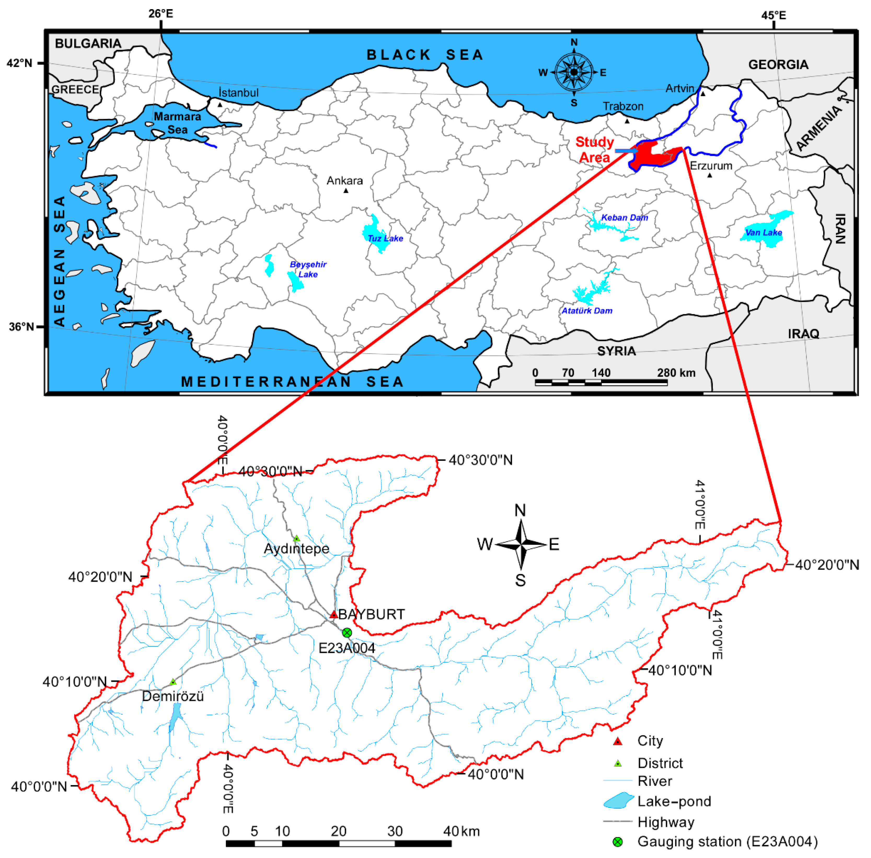
2.1. Basin Characteristics
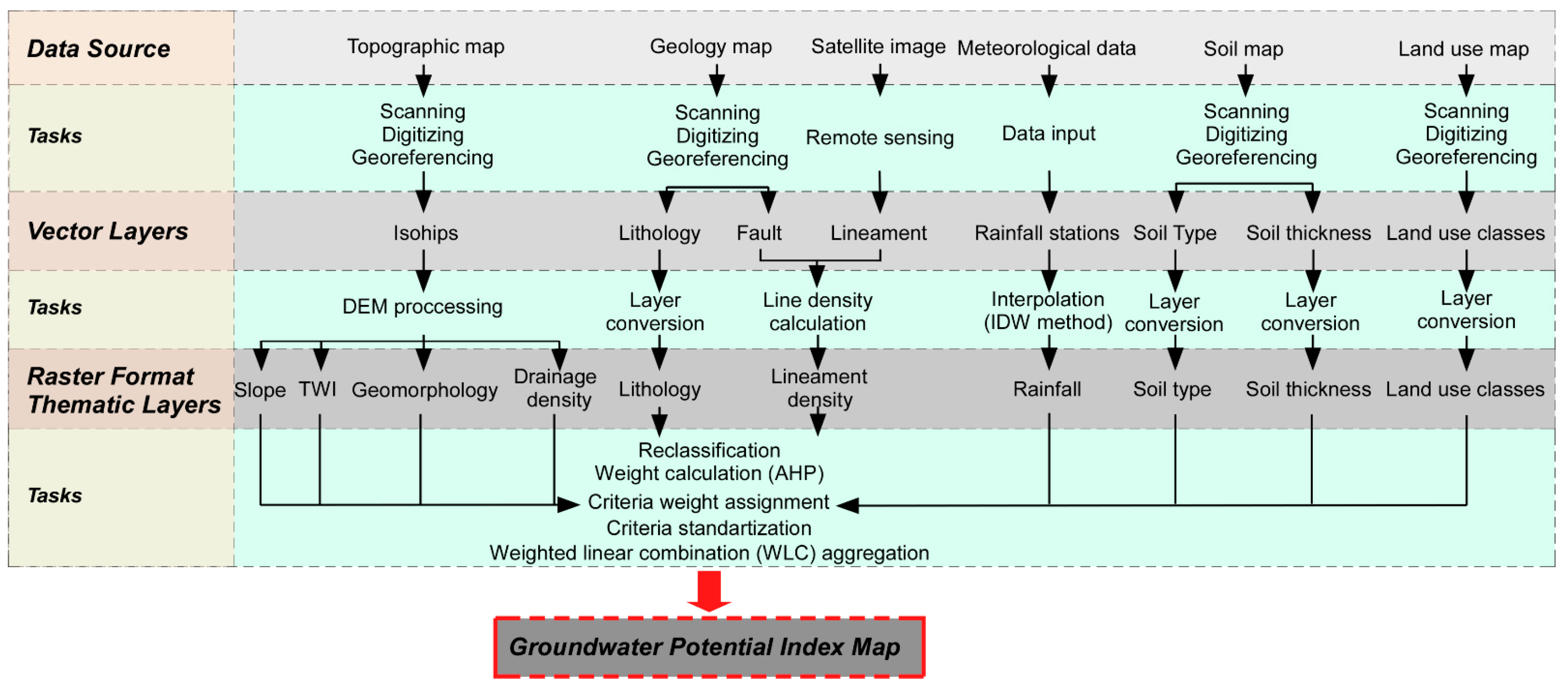
The Coruh River Basin is one of the 25 major river basins of Turkey. The Upper Coruh River Basin (UCRB) is the headwater basin in the Coruh River, and it covers an area of about 4000 km2 between latitudes 39°54′30.70″ to 40°31′16.34″ N and longitudes 39°40′06.43″ to 41°10′44.14″ E. A large part of UCRB is located in the Bayburt province (73.8%), and the remaining part lies in the Erzurum (21.4%), Gümüşhane (2.7%) and Erzincan (2.1%) province, NE Turkey (Figure 1).
The UCRB ranges from 1486 m to 3265 m, with slopes ranging from 0° to 64° (Figure 2a,b). The basic characteristics for the UCRB are presented in Table 1, and the ones about the current GWPZs modelling are given in Figure 2a‒f. The Coruh River, which has the third-highest runoff coefficients of the 25 major river basins in Turkey, originates in the Mescit Mountains in the Bayburt province. The river flows into the Black Sea after crossing through the Bayburt, Erzurum, Artvin, and Batumi-Georgia (the part of 22 km), respectively. The flow of the main Coruh River is perennial, and the observed mean daily discharge at the gauging station (E23A004) (see Figure 1) was 15.08 m3/s between the periods 3 September 1941 and 30 September 2015 [40]. Bayburt province reflects a transitional climate condition between the Eastern Black Sea climate and the Eastern Anatolian. The region is characterised by cool, dry summers and frigid, rainy winters. Based on the available meteorological data (for the 2000‒2019 period) from the station in the UCRB, the mean total annual precipitation is 470.35 mm, and annual air temperature is 7.85 °C at 1583 m amsl (Bayburt) [41]. For the whole UCRB, the mean total annual precipitation and mean total annual air temperature are computed as 588.73 mm and 7.75 °C, respectively (Table 1).
Pastures cover 58.33% of the study area, and approximately 32% of the UCRB consists of agricultural and arable lands, which are generally established on slopes of 0°‒20° (Figure 2b,e). The rest of the land-use classes consist of scrub, bare rock, forest, settlement, river, floodplain, and lake-pond, with total coverage of less than 10% (Table 1). The most dominant soil types are brown (62.37%) and maroon (28.86%) soils (Table 1), which respectively cover approximately < 2000 and > 2000 m (a.m.s.l.) portions of the UCRB (Figure 2c). The rest of the soil classes consist of alluvium, high-level mountain meadow, non-calcic brown, bare rock, basaltic, colluvium, non-calcic brown forest, brown forest, and floodplain, with a total area coverage of nearly 30% (Table 1). While the soil depth varies between 0 and 20 cm on the high and steep slopes, it is more than 90 cm in areas where the alluvial units are located on the flat or gentle slopes (Figure 2d).
The lithology of the basin is enclosed of metamorphic rocks that are the basement of the basin (gneiss), volcanic rocks (volcano-sedimentary; volcanite; dacite, rhyolite, rhyodacite), plutonic rocks (granitoid), ophiolitic rocks (ophiolite; ophiolitic mélange), and sedimentary rocks (clastic rock; clastic and carbonate rock; limestone; evaporite and sedimentary rock; travertine; alluvium) spanning in age from Paleozoic to Cenozoic (Figure 2f) [44,45]. The UCRB is located in the eastern Pontides belt and fragmented by faults, generally extending NE–SW (Figure 2f). Volcano sedimentary rocks are common in the northern part of the UCRB, and these rocks are separated from other units by a significant fault extended NE–SW in the middle part of the UCRB. Carbonate rocks are common in the south part of the UCRB. The areal coverages of different lithologic units in the UCRB are given in Table 1. Among the geological formations outcropping in the basin, ophiolitic rocks and flysch (Mesozoic), flysch (Eocene), terrestrial gypsum sediments (Oligocene), volcano-sedimentary rocks (Neogene), and clayey talus (Quaternary) formations are semi-permeable–impermeable formations [46]. Neogene terrestrial sediments and volcanic rocks cropping out in the basin are semi-permeable and poorly permeable geological formations, while the Paleozoic aged marbles, Mesozoic-, Eocene- and Neogene-aged limestones are porous and high-permeable geological formations [46]. Alluvial units formed by the accumulation of sediments carried by rivers have high permeability, and these units are highly permeable aquifers.

2.2. Methodology

2.2.1. Selecting of the Criteria Influencing Groundwater Storage Potential

Given local circumstances and data availability, the number of decision criteria used in the GWPZs determination process can vary within the regions [21,47,48]. In this study, ten different criteria controlling groundwater storage capacity (i.e., slope, topographic wetness index, geomorphology, drainage density, lithology, lineament density, rainfall, soil type, soil thickness, and land-use classes) were selected. These criteria were determined according to expert opinions and reviews of similar studies from the literature [34,39,49,50,51], depending on the conditions of the region and available data.

2.2.2. Data Acquisition and Integration into a GIS Database

In the present study, published topographic, geology, soil and land-use maps, the satellite images and meteorological data measured at the stations around the study area were used as the main data sources. Using these main data sources, the ten thematic maps (e.g., slope, topographic wetness index (TWI), geomorphology, drainage density, lithology, lineament density, rainfall, soil type, soil thickness and land-use classes) needed to create GWPZs map were generated in a GIS environment (ArcGIS 10.3.1. software) with regarding extensions.
The slope, TWI, geomorphology, and drainage density layers were generated using DEM. The DEM (consisting of cells 20 × 20 m in size) was created by digitising the isohips from 1/50,000 scaled topographic map sheets (Turkey G44 c‒d; H43 b‒c‒d; H44 a‒b‒c‒d; H45 a‒b‒c‒d; H46 a; I43 a‒b), which are published by the Turkish Ministry of National Defence, General Command of Mapping. The 3D analyst tool was used to obtain the slope layer. The slope is one of the terrain factors affecting the surface flow [52,53], and it directly controls the surface water infiltration to the aquifer [19]. While the groundwater potential is low in areas with high surface slopes, the groundwater potential is high in areas with low surface slopes [54].
The TWI is highly correlated with soil measure and groundwater level [55]. The higher value of TWI shows that the groundwater potential is also high [18]. The TWI layer was created using the following equation developed by Beven and Kirkby [56]:
TWI = ln (α/tan β)
where α is the upslope contributing area, and β is a topographic gradient. Geomorphology represents the landforms and topography, which are formed by winds, streams, etc., and it is one of the main factors related to the ground water potential [10,57,58,59]. In this study, the geomorphology layer was obtained based on DEM, using an extension named “Landform Classification” developed by Jenness [60], one of the topography tools [61] in ArcGIS.
The terrain transmissibility controls the drainage density. As the transmissibility decrease, the drainage density will increase, and as the transmissibility increases, the drainage density will decrease [62]. The drainage density layer of the UCRB was formed using the stream network with the line density tool (using Equation (2)). The stream network was delineated from DEM by following the steps of “fill DEM, flow direction, flow accumulation, stream order and stream to feature” respectively, in the hydrology toolset.
D d = i = 1 n D i A
where ΣDi is the total length of all streams in stream order i (km) and A is the watershed area (km2).
Geology is one of the main factors that control groundwater storage and movement in an aquifer [63]. Primary (the primary pores that are established when rocks are created) and secondary porosity (the effect of tectonism makes pores after the rocks have been deposited) of lithological units determine the presence and movement of water in the aquifer [64]. In this study, all lithologic units were weighted and ranked based on the available primary and secondary porosity and permeability. The lithology layer was derived from the 1/500,000 scaled geology maps, published by the General Directorate of Mineral Research and Exploration [44,45]. First, the geology map published in hard copy form was scanned and converted into a digital format. Afterwards, the lithology layer was obtained by performing georeferencing, heads-up digitisation and attribute data entry, respectively. Likewise, the faults (primary lineaments) in the study area were produced from the geology map. The lineaments layer was formed by combining the secondary lineaments (joints and fractures) obtained by the remote-sensing method. Then, the lineament density layer was created, using the line density method available in the spatial analyst tool (using Equation (3)).
L d = i = 1 n L i A
where Li is the length of the ith lineament, ΣLi is the total length of all lineaments (km), and A is the grid area (km2).
As mentioned above, lineaments create secondary porosity; hence they are a significant factor controlling the movement and presence of groundwater [16]. The areas with higher lineament density indicate the high potential of groundwater. Semi-automatic lineaments extraction was applied to Landsat-8 OLI imagery of the study area to obtain the secondary lineaments. First of all, the Gram–Schmidt pan-sharpening method was used on the satellite image to provide a more detailed image, and the image resolution increased from 30 m to 15 m. Then, the principal component analysis (PCA) method was applied, using ENVI 5.3 software to clarify the lineaments. The lineaments were extracted from the image obtained after the PCA (PC1) application with the LINE module of PCI Geomatica software. Lineaments caused by human effects (such as roads and land borders) and morphological impact (such as stream channels and drainage divisions) were removed, using detailed geology, topography and satellite images to obtain more realistic lineament data. Finally, these lineament data were transferred to ArcGIS software.
Rainfall is the primary water source on the earth, and it controls the surface and groundwater amount [65,66,67]. For this reason, it is widely used in groundwater potential determination studies [11,68,69,70]. The total annual rainfall amount (between the periods of 1981 and 2019 [41]) obtained from six meteorology stations (Bayburt, Trabzon, Rize, Erzurum, Erzincan and Gümüşhane) around the study area were used to create the rainfall layer. The rainfall amounts were entered to related stations as attribute data, and the rainfall layer was created, using the Inverse Distance Weighting (IDW) interpolation method available in 3D Analyst tools. The power and number of points for IDW method were selected as the default numbers in ArcGIS software, 2 and 12, respectively.
Soil type and thickness play an essential role in water recharge to the aquifer [32,51]. The water infiltration and soil permeability primarily depend on the soil texture and thickness, and these factors assist the characterisation of the GWPZs [71]. Soil type and soil thickness layers were obtained from the 1/25,000 scaled soil characteristics map of Turkey [42]. The map in hard copy format was converted into a digital form by scanning and georeferenced, then the soil type and soil thickness layers were created by hand-up digitisation and entering the attribute data. First order polynomial (Affine) transformation was applied for the georeferencing of the maps. The same application steps, in a similar manner, were applied to a 1/25,000 scaled land-use types map of Turkey [43], and the land-use layer was generated. The land use and landscape are highly related to groundwater in both the aspect of quality and quantity due to the impact on evapotranspiration, drainage, and recharging of the groundwater system [72,73].
All data layers were georeferenced within the GIS environment, using the Universal Transverse Mercator (UTM), World Geodetic System (WGS 1984) and 37N Zone Projection System. All obtained layers in vector format were converted into the raster format consisting of cells 20 × 20 m in size. The methodology used in creating the GIS data layers and groundwater potential zones (GWPZs) map is depicted in Figure 3.

2.2.3. Weight Assignment and Normalisation of Criteria Using AHP

AHP, developed by Saaty [31] is a decision support tool that is widely used in making complex decisions based on the pairwise comparison. The first step of the AHP methodology is selecting the important criteria for the goal decision and creating a pairwise comparison matrix based on expert opinions or judgment between the criteria chosen [74]. With this pairwise comparison matrix (see Equation (4)), the complex decision-making process between the criteria is reduced to a single level, and the relative importance values of the criteria concerning each other are obtained. When comparing the criteria, Saaty’s 1‒9 importance scale shown in Table 2 is used.
A   = [ a 11 a 12 a 13 a a 1 n a 21 a 22 a 23 a a 2 n a 31 a 32 a 33 a a 3 n a a a a a n a n 1 a a a a n n ]
where an displays the nth indicator unit, and ann is the judgment matrix element.
The second step of the AHP calculations is to determine the normalised weights, using the criteria’ geometric mean, as shown in Equation (5).
W n = G m n 1 n G m
where W is the Eigen vector and Gm is the geometric mean of the ith row of the judgement.
The last step of the AHP method is to test the consistency of the normalised criterion weights. For this, the consistency ratio (CR) is calculated using Equation (6), given below. For the weights to be considered consistent, the CR value must be less than 0.10. If the CR value is above 0.10, the pairwise comparisons must be re-evaluated.
C R = C I R I
where CR is the consistency ratio, CI is the consistency index calculated using Equation (7), and RI is the random consistency index (see Table 3 given by Saaty [31]).
C I = λ m a x n n 1
where λmax is the maximum eigenvalue of the judgment matrix, calculated using Equation (8).
λ m a x = 1 n i = 1 n ( A w ) i w i
The pairwise comparison matrix, standardised rating and normalised weight values of the criteria and its sub-criteria used in this study are shown in Table 4 and Table 5. The consistency ratios (CR) of the pairwise comparisons are determined to be less than 0.1, and the CR values of the criteria are shown in Table 6, together with the values of λmax, CI and RI.

2.2.4. Criteria Standardisation, Delineation and Validation of Groundwater Potential Zones Map

Data standardisation is widely used in GIS-based decision support studies together with AHP, and it reduces all decision criteria to a common scale of measurement [35,39,47,48,59,75]. In this study, the rating values ranging from 1 to 5 (very low, low, moderate, high and very high) were assigned to standardise each raster GIS-based criteria map (see Table 5 and Figure 4).
After assigned rating and weight values to all criteria and determined to be consistent, the weighted linear combination (WLC) aggregation method [76] was used to prepare the groundwater potential index (GWPI) for UCRB. Equation (9) of GWPI is shown below:
G W P I = i = 1 n w i × r i
where n is the number of criteria, wi is the relative weight of criterion i and ri is the standardised rating of criterion i.

3. Results

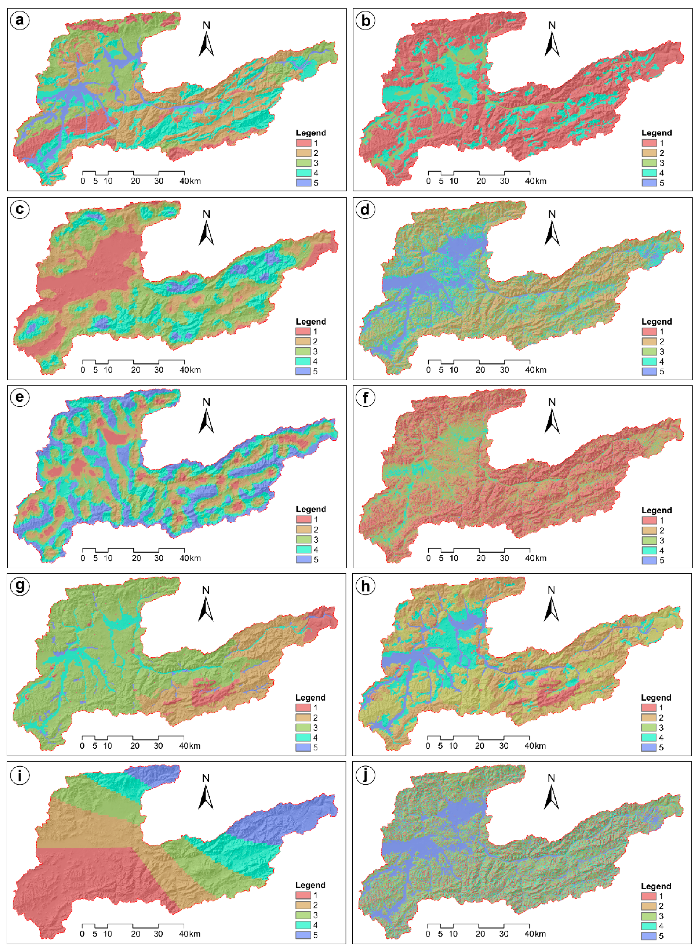
3.1. Thematic Layers Produced Using AHP Method

The results of AHP calculations of ten main criteria and their sub-criteria used in this study and the standardised rating values (ri) are shown in Table 4 and Table 5. Additionally, the thematic layers created using standardised rating values (ri) of the main criteria are shown in Figure 5. Information on the layers is detailed below. The following sections provide details of the produced thematic layers for GWPZs in this study.

3.1.1. Lithology

The lithology is the most important criterion, with the relative weight (Wi) of 0.222 used to determine GWPZs of UCRB (Table 4). The relative weight (wi) values of these units in descending order were determined as alluvium, clastic rock, clastic and carbonate rock, volcano-sedimentary rock, volcanite, travertine, limestone, evaporite sedimentary rock, ophiolite, ophiolitic mélange, gneiss, dacite‒rhyolite‒rhyodaicte and granitoid (Table 5). Alluvium was ranked with the standardised ranking (ri) value of “5” representing a very high potential for groundwater storage. In contrast, the clastic rock and carbonate rock were ranked with “4” (high potential), volcanite and volcano-sedimentary rock were ranked with “3” (moderate potential), travertine, limestone and evaporate sedimentary rock were ranked with “2” (low potential), and granitoid and dacite, rhyolite, rhyodacite were ranked with “1” (very low potential) (Figure 4a). These ranking classes occupy the UCRB area of 9.70%, 23.54%, 23.44%, 31.93% and 11.39%, respectively.

3.1.2. Land-Use Classes

The relative weight (Wi) of land-use classes is 0.045, ranking 8th among the criteria used for GWPZs determination of UCRB (Table 4). The water bodies (lake-pond and river) have the highest relative weight (wi) and ranking (ri) values. In descending order of relative weight (wi), the rest of the land-use classes were listed as floodplain, agriculture, arable land, forest, scrub, pasture, bare rock and settlement areas (Table 5). The land-use classes were rated with “5” for lake-pond and river (very high potential), “4” for floodplain and agriculture (high potential), “3” for arable land (moderate potential), “1” for the forest, scrub, pasture, bare rock and settlement (very low potential), based on standardised rating value (ri) (Figure 4b). These rating classes cover 0.08%, 22.97%, 8.94% and 68.01% of the study area, respectively. In the weighting and rating of land-use classes, rates of recharge, evapotranspiration and runoff, which help provide the infiltration rate in classes, were considered.

3.1.3. Lineament Density

Lineament density takes place in 4th order with 0.091 Wi in relative weighting among the criteria used for determining GWPZs in this study (Table 4). The primary lineaments in UCRB, especially faults, trended in the NE–SW direction (Figure 2f). The lineament density value of UCRB varied between 0 and 2.77 km/km2 in the study area, and the lineament density was classified into five groups. The ranking classes of “1” to “5” (Figure 4c) occupy the UCRB areas of 22.15%, 24.47%, 30.67%, 19.23% and 3.48%, respectively.

3.1.4. Slope

Slope ranks 6th with 0.074 (Wi) in terms of relative importance on GWPZs determination among the criteria selected in this study (Table 4). The slope of UCRB was divided into five groups as 0°–4° (very high potential), 4°–10° (high potential), 10°–20° (moderate potential), 20°–40° (low potential) and more than 40° (very low potential) with increasing relative weight (wi) and rating (ri) values (Table 4, Figure 4d). The rating classes signed with the rate of “1” to “5” cover an area of 0.25%, 30.79%, 33.86%, 16.20% and 18.90% of the UCRB.

3.1.5. Drainage Density

The drainage density values vary between 0 and 1.38 km/km2 in the UCRB. Drainage density occurs 5th with 0.089 (Wi) in terms of relative importance on GWPZs determination among the criteria selected in this study (Table 4). The drainage density was divided into five classes in the UCRB. The rating values (ri) of the drainage density classes vary from 1 to 5 (Figure 4e) with increasing relative weighting values (wi) (Table 5). The high potential rating class (ri = 5) occupies an area of 25.3% of UCRB, while the rating classes of “4”, “3”, “2” and “1” cover an area of 26.7%, 23.91%, 17.6% and 6.4%, respectively.

3.1.6. Topographic Wetness Index (TWI)

The topographic wetness index (TWI) value ranges between 2.71 and 26.87 in the UCRB. The (TWI) is the second most important criterion among the criteria (with the 0.129 Wi) used in this study in terms of relative weighting (Wi) on GPWZs (Table 4). The TWI of the UCRB was categorized into five classes as very low potential (ri = 1, wi = 0.049), low potential (ri = 2, wi = 0.078), moderate potential (ri = 3, wi = 0.145), high potential (ri = 4, wi = 0.219) and very high potential (ri = 5, wi = 0.508) (Table 5). The areas with high TWI are commonly located in the west of the study area, while the areas in the north of the study area have lower TWI (Figure 4f).

3.1.7. Soil Type

Soil type is the 7th most important criterion among the criteria used to determine GWPZs in this study regarding relative weighting (Table 4). These soil type classes were weighted and rated according to their permeability, varying depending on grain sizes. The relative weight (wi) values of soil type classes in descending order were defined as colluvium (0.256), floodplain (0.197), alluvium (0.177), non-calcic brown forest soil (0.070), non-calcic brown soil (0.066), brown soil (0.062), high-level mountain meadow (0.049), brown forest soil (0.048), maroon (0.032), basaltic (0.022) and bare rock (0.015) (Table 4). While the colluvium has the highest rating value (ri = 5), the rating of alluvium and floodplain is “4”, the rating of non-calcic brown forest soil, non\-calcic brown soil, brown soil, high-level mountain meadow and brown forest soil is “3”, the rating value of maroon is “2”, and the rating value of basaltic and bare rock is “1” (Table 5); the covered area of these ranking classes in the UCRB are 2.29%, 8.65%, 61.64%, 20.93% and 6.47%, respectively. Rating and relative weighting values are lower in the areas located to the east of UCRB (Figure 4g).

3.1.8. Soil Thickness

Soil thickness is the 9th most important criterion, with the 0.022 Wi value among the criteria used to determine GWPZs in this study in terms of relative weighting (Table 4). The soil thicknesses of UCRB were divided into five distinct classes as 0 cm, 0–20 cm, 20–50 cm, 50–90 cm, and more than 90 cm, with assigned ratings (ri) of “1”, “2”, “3”, “4” and “5”, respectively (Figure 4h). Relative weighting (wi) of 0 cm, 0–20 cm, 20–50 cm, 50–90 cm classes are 0.035, 0.080, 0.150, 0.227 and 0.508 ( Table 5) and these classes cover an area of UCRB of 3.95%, 34.92%, 34.36%, 17.09% and 9.66%, respectively. While the soils on the steep parts of mountain areas in UCRB are thinner, the soils on the gentle slope or flat parts are thicker.

3.1.9. Rainfall

Rainfall is the 3rd most crucial criterion, with the 0.099 Wi value among the criteria used to determine GWPZs in this study in terms of relative weighting (Table 5). The mean annual rainfall of the UCRB varies between 282 mm and 1196 mm, and it was categorised into five different classes (Table 5). The ratings of these classes range from “1” to “5”, and the relative weighting (wi) increases in parallel to the rating values (ri). The annual average rainfall values show the lower amount in the SW parts of the UCRB, whereas the mean annual rainfall amount increases towards the NE parts of the UCRB (Figure 4i).

3.1.10. Geomorphology

Geomorphology is the least important criterion, with the relative weight (Wi) of 0.015 used to determine GWPZs of UCRB (Table 4). There are four different geomorphology classes in the UCRB (Table 5): valley, pediplain, escarpment and high ridge. These classes cover an area of UCRB of 22.51%, 17.68%, 35.11% and 24.67%, respectively. According to its percolation characteristics and groundwater storage capacities, the “pediplain” class has the higher relative weighting (w i= 0.490) and rating (ri = 5) values, while the “high ridge” class has the lowest weighting (wi = 0.079) and rating (ri = 1) values (Table 5, Figure 4j). Pediplain is mostly located in the western parts of the UCRB (Figure 4j).

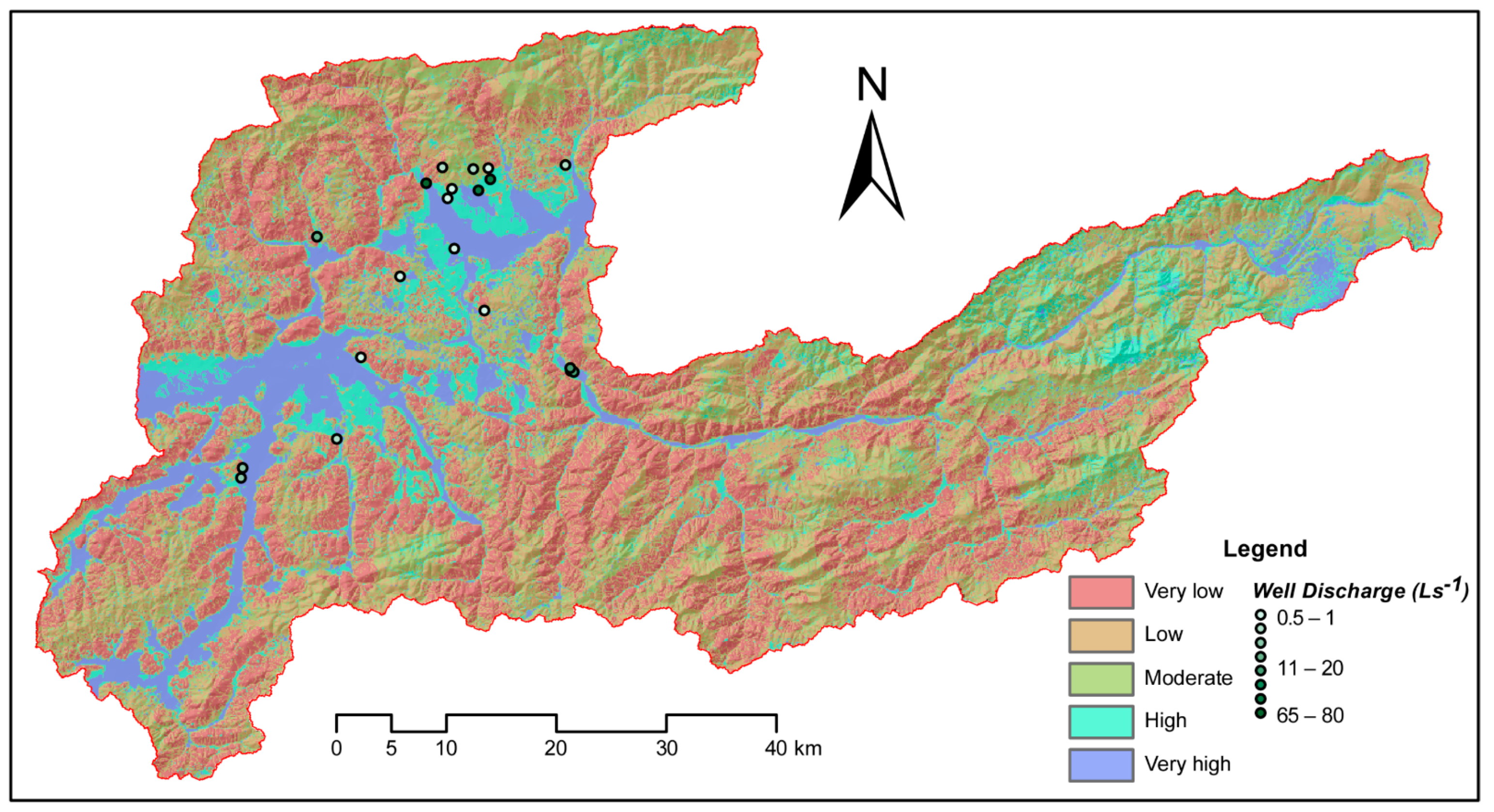
3.2. Delineation and Validation of Groundwater Potential Zones

In this study, each of the ten criteria layers representing the GWPZs determination criteria was separately rated (Figure 4) and multiplied by the AHP-derived criteria weights (Table 4 and Table 5) and finally summed up on a cell-by-cell basis to create the GWPZs map of the Upper Coruh River Basin (NE Turkey). The final GWPI values obtained with the weighted linear combination (WLC) method for UCRB vary from 0.073 to 1.73. The resulting GWPZs map are divided into five suitability classes, namely, very low potential, low potential, moderate potential, high potential and very high potential, using the natural breaks (Jenks) algorithm (Figure 5).
The measured discharges and depth to groundwater (bgl; below ground level) data (obtained from the Turkish General Directorate of State Hydraulic Works) related to the 22 groundwater wells located in the different parts of the study area (Figure 5) were used to validate the groundwater potential zones. The discharges of wells located in the study area range between 0.5 Ls−1 and 80 Ls−1 and the depth to groundwater vary between 0 and 90 m (Table 7). The data reveal that seven of the wells exist in the “very high potential” zone, three of the wells exist in the “high potential” zone, four of the wells exist in the “moderate potential” zone, six of the wells exist in the “low potential” zone, and two of the wells exist in the “very low potential” zone (Table 7). The discharges of the wells that existed in the “very high potential” zone vary between 9 Ls−1 and 80 Ls−1 with a mean of 32.4 Ls−1, and the groundwater depths range from 0.5 m to 2.1 m with a mean of 1.44 m. The mean discharge of the wells falling on the “high potential” zone is 27 Ls−1 (min: 8 Ls−1, max: 65 Ls−1), and the mean groundwater depth is 17.6 m (min: 0.5 m, max: 28 m). The mean discharge of the wells falling on the “moderate potential” zone is 3.35 Ls−1 (minimum: 0.5 Ls−1, maximum: 11.9 Ls−1) and the mean groundwater depth is 72.5 m (min: 20 m, max: 90 m). The mean discharge of the wells that existed in the “low potential” zone 0.75 Ls−1 (min: 0.5 Ls−1, max: 0.1 Ls−1) and the mean groundwater depth is 63.7 m (min: 32 m, max: 88 m). The mean discharge of the wells that existed in the “very low potential” zone 0.75 Ls−1 (min: 0.5 Ls−1, max: 0.1 Ls−1) and the mean groundwater depth is 87.5 m (min: 85 m, max: 90 m).

4. Discussion

The GWPZs classes of very low, low, moderate, high and very high potentials occupy the area of 25.1%, 32.05%, 21.4%, 11.4% and 10.1% in the UCRB, respectively. While high-potential areas commonly occupy the places in the eastern part of the study area, very-high-potential areas are concentrated in the western part of the UCRB (Figure 5). The GWPZs map of UCRB obtained from the GIS and AHP analysis is acceptable once compared to the depth to groundwater and discharge data of wells located in the study area. Similarly, in the literature, the results of many studies have shown that the GWPZs derived by the GIS and AHP methods strongly overlap with the yield and discharge of the wells located in the given area [10,18,39,46,50].
Lithology directly controls the infiltration and percolation. That is why it is a highly significant parameter for determining groundwater potential [18,68,77]. The lithologic units’ high permeability and porosity increase groundwater storage and groundwater yields [78]. According to structural and lithological characteristics (such as porosity and permeability) of the geological formations around the study area, granite, granitoid, dacite–rhyolite–rhyodacite, ophiolite, and ophiolitic mélange units are mostly impermeable formations; evaporite sedimentary, limestone, volcanite, and volcano-sedimentary units are low permeable–impermeable formations; clastic and carbonate units are semi-permeable formations; unconfined quaternary units are defined as permeable formations [46]. The unconsolidated sediments (e.g., alluvium) in the study area existed in the very-high-potential class of the GWPZs map. These sediments have high porosity and permeability and are classified into a very-high-potential in similar studies [19,49]. Conversely, studies reveal that igneous rocks (such as granite, granitoid, dacite–rhyolite–rhyodacite) are classified as having very low potential due to their non-permeability or very low permeability [10,19].
Land-use condition is one of the most crucial factors affecting surface runoff because of the evapotranspiration, infiltration and evaporation depending on agents such as surface vegetation and soil moisture. Therefore, it highly affects groundwater recharge. Water bodies (e.g., lake, pond and river) are the permanent source for groundwater recharge. Thus, these areas are the most crucial groundwater potential areas [32,49]. Conversely, settlement and bare lands mainly generate the surface runoff process and have decreased water recharge from the surface downward. Therefore, these factors’ importance on groundwater recharge and storage is very low [19,35,68]. Agricultural and floodplain lands have more porosity, increasing water percolation into the subsurface; hence, these factors have moderately high to high potential for groundwater storage [69,70]. The arable land and agricultural land largely overlap with the high and very high potential classes of the GWPZs map of the UCRB. This result is similar to previous studies [16,34,35].
Lineament (such as faults, joints and fractures) is the parameter that directly affects permeability. Water movement is higher in areas with high lineament density, so the groundwater potential is also higher in these areas and vice versa [25]. In the GWPZ map obtained from this study, the lineament density classes of regions with high well discharges vary from low to high potential. The previous studies’ results also show a strong correlation between lineament intersections and well yields [79,80].
The terrain slope directly affects the surface runoff process; hence, it has an essential role in groundwater recharge [68]. The finding of previous studies showed that the low slope areas have a high potential for groundwater storage due to the longer residence time for water to percolate. In contrast, the high slope areas have lower groundwater potential because of the quick surface runoff from the terrain [19,81,82]. In this study, it is seen that the mean slope of very low and low potential classes of GWPZs of UCRB is 19°, whereas the mean slope of high and very high potential classes of GWPZs of UCRB is 3°.
Drainage density is an important factor prevailing the water movement and infiltration into the aquifer [24]. High permeability sub-soil material results in low drainage density [83]. Hence, low drainage density areas have high groundwater potential and vice versa [24,84]. This study also shows that 77% of the wells (with a mean discharge of 13.7 Ls−1) used for validation scattered in the UCRB are located in moderate and high potential areas for groundwater.
The topographic wetness index (TWI) is a secondary topographic index depending on the local slope gradient that reveals drainage potential. It is highly related to soil depth and soil texture [85]. Studies have shown that high TWI areas have high groundwater potential, while low TWI areas have low groundwater potential [22,39,49]. This study also revealed that the mean TWI is 7.4 of the high and very high potential classes of GWPZs of UCRB, whereas the mean TWI is 4.8 of the very low and low potential classes of GWPZs of UCRB.
Soil type affects the rate of water infiltration into the ground depending on the processes of saturation or desaturation of the pores [50]. The porosity of the soil classes controls the water movement into the subsurface. The groundwater potential is higher in the soil type that has a coarse-grained structure (e.g., sandy soil), while the groundwater potential is lower in the fine-grained structured soil type (e.g., loamy soil) [19,21]. Approximately 90% of the high and very high potential areas of the GWPZ classes of the UCRB are covered by alluvium (36%), brown soil (35%), maroon (13%) and colluvium (7%). On the other hand, nearly 90% of the low and very low potential areas are covered by brown soil (58%), maroon (20), high-level mountain meadow (7%) and bare rock (5%) soil classes. The porosity of colluvium and alluvium soil classes is higher than the other soil class covers in UCRB due to their coarse-grains. Therefore, the groundwater potential is higher in these areas [21,35]. Similarly, soil thickness is also an essential factor for groundwater potential in terms of the volume of infiltration and the water infiltration time to reach the groundwater table [86]. Thicker soils are susceptible to low surface runoff; hence, the infiltration capacity is high in these units. In contrast, bare rocks and thin soils are vulnerable to increased surface runoff. Thus, the groundwater potential is low in these units [25,50,86]. In the high potential class of GWPZs of UCRB, 41% of the area has a soil thickness of more than 90 cm, 31% of the area has a soil thickness of 50–90 cm, 16% of the area has a soil thickness of 20–50 cm and 12% of the area has a soil thickness of 0–20 cm. On the contrary, in the low and very low potential classes of GWPZs of UCRB, the areas of these classes are 1%, 13%, 40% and 46%, respectively.
The annual mean rainfall amounts of GWPZs of UCRB are 576 mm for the high and very high potential zone, whereas they are 552 mm for the low and very low potential zone. The previous studies have shown that the high amount of rainfall results in groundwater’s high potential, due to a big amount of water percolating to the ground [25,87].
The valleys formed due to the rivers’ incising action contain rocks and sediments with high permeability, where the water quickly infiltrates to the ground [88]. The pediplain is a spacious flat area formed by the unification of pediments [89] and represents a highly permeable unit promoting water recharge and percolation, thus the high potential of groundwater [69]. Escarpment and high ridges are typically associated with poor infiltration capacities or being unsuitable for groundwater occurrence [24,90]. In the high and very high GWPZ classes of UCRB, the pediplain geomorphology unit covers an area of 78% while it covers an area of 5% in low and very low GWPZ classes of UCRB. The valley, escarpment and high-ridge units cover an area of 16%, 5% and 3% in the high and very high GWPZ classes of UCRB, respectively, whereas they occupy an area of 17%, 46% and 36% in the low and very low GWPZ classes of UCRB.

5. Conclusions

In this study, the groundwater potential was explored using an integrated approach of GIS and MCDM for the Upper Coruh River Basin (UCRB). The AHP technique was selected for the multi-criteria decision analysis between the main criteria (and their sub-criteria) affecting the groundwater potential of the basin. As the main criteria, lithology, land-use classes, lineament density, slope, drainage density, topographic wetness index, soil type, soil thickness, rainfall and geomorphology layers were chosen, appraised and explicated. These criteria were weighted both within themselves and with each other by making pairwise comparisons and were collected in the GIS environment, using the WLC method. Thus, the groundwater potential zones map of the study area was created.
The groundwater potential zones map were classified into five different classes, namely, very high potential, high potential, moderate potential, low potential and very low potential. Finally, the derived groundwater potential zones map was compared with the measured discharges and depths to groundwater of groundwater wells scattered over the UCRB to test its accuracy. The mean discharges and mean depths to groundwater of the wells are 32.4 Ls−1 and 1.44 m for very high potential zones; 27 Ls−1 and 17.6 for high potential zones; 3.35 Ls−1 and 72.5 for the moderate potential zones; 0.75 Ls−1 and 63.7 for low potential zones; and 0.75 Ls−1 and 87.5 m for very low potential zones, respectively. These results reveal that the GWPZs map created by the GIS integrated MCD method are quite accurate. Very high groundwater potential zones are primarily covered in the middle of the western reaches of the UCRB. However, these zones are located also around the stream channel by overlapping the sediments carried by streams (such as alluvium and floodplain). The very high groundwater potential zones cover 10.1% of the study area. Over the eastern part of the UCRB, predominantly high and moderate groundwater potential zones are situated. However, these zones are spread over the study area and cover an area of 11.4% and 21.4%, respectively. Low and very low groundwater potential zones extend over the catchment and cover an area of 32.05% and 25.1%, respectively. The depicted GWPZs map was validated, using the discharge data of wells located in the study area.
The existence of industrial areas in the region is quite limited, and the people of the region earn their living from agriculture and animal farming, as job opportunities are restricted. Agricultural activity areas cover 31.88% of the study area. Considering these conditions, the groundwater potential zones map delineated result of this study will provide policymakers and local authorities with a prediction in groundwater management for agricultural and urban utilisation. Additionally, the methodology used in this study will help other scientists for similar studies around the world.

Funding

This research received no external funding.

Institutional Review Board Statement

Not applicable.

Informed Consent Statement

Not applicable.

Data Availability Statement

The author involved approves the availability of the data obtained from this study. In addition, the GIS input data used for the GWPZs delineation presented in this study are available upon request from the author.

Acknowledgments

The discharge data of wells located in the study area, which were used for the validation, were obtained from “Turkey General Directorate of State Hydraulic Works” and the meteorological data were obtained from “Turkish State Meteorological Service”.

Conflicts of Interest

The author declares no conflict of interest.

References

  1. GDSHW (General Directorate of State Hydraulic Works)—A. Toprak Su Kaynakları. Available online: https://www.dsi.gov.tr/Sayfa/Detay/754 (accessed on 15 February 2021).
  2. GDWM. The Effect of Climate Change on Water Resources Project Report; Republic of Turkey Ministry of Agriculture and Forestry–General Directorate of Water Management: Ankara, Turkey, 2016; p. 424. (In Turkish) [Google Scholar]
  3. UNECE (United Nations Economic Commission for Europe). Second Assessment of Transboundary Rivers, Lakes and Groundwaters; United Nations Publications: New York, NY, USA, 2011. [Google Scholar]
  4. De Stefano, L.; Lopez-Gunn, E. Unauthorised groundwater use: Institutional, social and ethical considerations. Water Policy 2012, 14, 147–160. [Google Scholar] [CrossRef] [Green Version]
  5. Israil, M.; Al-Hadithi, M.; Singhal, D.C. Application of a resistivity survey and geographical information system (GIS) analysis for hydrogeological zoning of a piedmont area, Himalayan foothill region, India. Hydrogeol. J. 2006, 14, 753–759. [Google Scholar] [CrossRef]
  6. Razandi, Y.; Pourghasemi, H.R.; Neisani, N.S.; Rahmati, O. Application of analytical hierarchy process, frequency ratio, and certainty factor models for groundwater potential mapping using GIS. Earth Sci. India 2015, 8, 867–883. [Google Scholar] [CrossRef]
  7. Bhattacharya, S.; Das, S.; Das, S.; Kalashetty, M.; Warghat, S.R. An integrated approach for mapping groundwater potential applying geospatial and MIF techniques in the semiarid region. Environ. Dev. Sustain. 2021, 23, 495–510. [Google Scholar] [CrossRef]
  8. Nampak, H.; Pradhan, B.; Manap, M.A. Application of GIS based data driven evidential belief function model to predict groundwater potential zonation. J. Hydrol. 2014, 513, 283–300. [Google Scholar] [CrossRef]
  9. Şener, E.; Şener, Ş.; Davraz, A. Groundwater potential mapping by combining fuzzy-analytic hierarchy process and GIS in Beyşehir Lake Basin, Turkey. Arab. J. Geosci. 2018, 11, 187. [Google Scholar] [CrossRef]
  10. Murmu, P.; Kumar, M.; Lal, D.; Sonker, I.; Singh, S.K. Delineation of groundwater potential zones using geospatial techniques and analytical hierarchy process in Dumka district, Jharkhand, India. Groundw. Sustain. Dev. 2019, 9, 100239. [Google Scholar] [CrossRef]
  11. Forootan, E.; Seyedi, F. GIS-based multi-criteria decision making and entropy approaches for groundwater potential zones delineation. Earth Sci. Inform. 2021, 14, 333–347. [Google Scholar] [CrossRef]
  12. Solomon, S.; Quiel, F. Groundwater study using remote sensing and geographic information systems (GIS) in the central highlands of Eritrea. Hydrogeol. J. 2006, 14, 1029–1041. [Google Scholar] [CrossRef] [Green Version]
  13. Chowdary, V.M.; Ramakrishnan, D.; Srivastava, Y.K.; Srivastava, Y.K.; Chandran, V.; Jeyaram, A. Integrated water resource development plan for sustainable management of Mayurakshi Watershed, India using remote sensing and GIS. Water Resour. Manage. 2009, 23, 1581–1602. [Google Scholar] [CrossRef]
  14. Mukherjee, P.; Singh, C.K.; Mukherjee, S. Delineation of groundwater potential zones in arid region of India—A remote sensing and GIS Approach. Water. Resour. Manag. 2012, 26, 2643–2672. [Google Scholar] [CrossRef]
  15. Awawdeh, M.; Obeidat, M.; Al-Mohammad, M.; Al-Qudah, K.; Jaradat, R. Integrated GIS and remote sensing for mapping groundwater potentiality in the Tulul al Ashaqif, Northeast Jordan. Arab. J. Geosci. 2014, 7, 2377–2392. [Google Scholar] [CrossRef]
  16. Yeh, H.F.; Cheng, Y.S.; Lin, H.I.; Lee, C.H. Mapping groundwater recharge potential zone using a GIS approach in Hualian River, Taiwan. Sustain. Environ. Res. 2016, 26, 33–43. [Google Scholar] [CrossRef] [Green Version]
  17. Swetha, T.V.; Gopinath, G.; Thrivikramji, K.P.; Jesiya, N.P. Geospatial and MCDM tool mix for identification of potential groundwater prospects in a tropical river basin, Kerala. Environ. Earth. Sci. 2017, 76, 428. [Google Scholar] [CrossRef]
  18. Achu, A.L.; Thomas, J.; Reghunath, R. Multi-criteria decision analysis for delineation of groundwater potential zones in a tropical river basin using remote sensing, GIS and analytical hierarchy process (AHP). Groundw. Sustain. Dev. 2020, 10, 100365. [Google Scholar] [CrossRef]
  19. Allafta, H.; Opp, C.; Patra, S. Identification of groundwater potential zones using remote sensing and GIS techniques: A case study of the Shatt Al-Arab Basin. Remote Sens. 2021, 13, 112. [Google Scholar] [CrossRef]
  20. Keeney, R.L.; Wood, E.F. An illustrative example of the use of multi attribute utility theory for water resource planning. Water Resour. Res. 1977, 13, 705–712. [Google Scholar] [CrossRef]
  21. Çelik, R. Evaluation of Groundwater Potential by GIS-Based Multicriteria Decision Making as a Spatial Prediction Tool: Case Study in the Tigris River Batman-Hasankeyf Sub-Basin, Turkey. Water 2019, 11, 2630. [Google Scholar] [CrossRef] [Green Version]
  22. Mallick, J.; Khan, R.A.; Ahmed, M.; Alqadhi, S.D.; Alsubih, M.; Falqi, I.; Hasan, M.A. Modeling groundwater potential zone in a semi-arid region of Aseer using Fuzzy-AHP and geoinformation techniques. Water 2019, 11, 2656. [Google Scholar] [CrossRef] [Green Version]
  23. Rajasekhar, M.; Raju, G.S.; Sreenivasulu, Y.; Raju, R.S. Delineation of groundwater potential zones in semi-arid region of Jilledubanderu river basin, Anantapur District, Andhra Pradesh, India using fuzzy logic, AHP and integrated fuzzy-AHP approaches. HydroResearch 2019, 2, 97–108. [Google Scholar] [CrossRef]
  24. Etikala, B.; Golla, V.; Li, P.; Renati, S. Deciphering groundwater potential zones using MIF technique and GIS: A study from Tirupati area, Chittoor District, Andhra Pradesh, India. HydroResearch 2019, 1, 1–7. [Google Scholar] [CrossRef]
  25. Raju, R.S.; Raju, G.S.; Rajasekhar, M. Identification of groundwater potential zones in Mandavi River basin, Andhra Pradesh, India using remote sensing, GIS and MIF techniques. HydroResearch 2019, 2, 1–11. [Google Scholar] [CrossRef]
  26. Lilienfeld, A.; Asmild, M. Estimation of excess water use in irrigated agriculture: A Data Envelopment Analysis approach. Agric. Water Manag. 2007, 94, 73–82. [Google Scholar] [CrossRef]
  27. Alamanos, A.; Mylopoulos, N.; Loukas, A.; Gaitanaros, D. An Integrated multicriteria analysis tool for evaluating water resource management strategies. Water 2018, 10, 1795. [Google Scholar] [CrossRef] [Green Version]
  28. Roozbahani, A.; Ebrahimi, E.; Banihabib, M.E.A. Framework for ground water management based on bayesian network and MCDM Techniques. Water Resour. Manage. 2018, 32, 4985–5005. [Google Scholar] [CrossRef]
  29. Arabameri, A.; Rezaei, K.; Cerda, A.; Lombardo, L.; Rodrigo-Comino, J. GIS-based groundwater potential mapping in Shahroud plain, Iran. A comparison among statistical (bivariate and multivariate), data mining and MCDM approaches. Sci. Total Environ. 2019, 658, 160–177. [Google Scholar] [CrossRef]
  30. Sapkota, M.; Arora, M.; Malano, H.; Sharma, A.; Moglia, M. Integrated evaluation of hybrid water supply systems using a PROMETHEE–GAIA approach. Water 2018, 10, 610. [Google Scholar] [CrossRef] [Green Version]
  31. Saaty, T.L. The Analytic Hierarchy Process; McGrawHill: New York, NY, USA, 1980. [Google Scholar]
  32. Jhariya, D.C.; Kumar, T.; Gobinath, M.; Diwan, P.; Kishore, N. Assessment of groundwater potential zone using remote sensing, GIS and multi criteria decision analysis techniques. J. Geol. Soc. India 2016, 88, 481–492. [Google Scholar] [CrossRef]
  33. Andualem, T.G.; Demeke, G.G. Groundwater potential assessment using GIS and remote sensing: A case study of Guna tana landscape, upper blue Nile Basin, Ethiopia. J. Hydrol. Reg. Stud. 2019, 24, 100610. [Google Scholar] [CrossRef]
  34. Fenta, A.A.; Kifle, A.; Gebreyohannes, T.; Hailu, G. Spatial analysis of groundwater potential using remote sensing and GIS-based multi-criteria evaluation in Raya Valley, northern Ethiopia. Hydrogeol. J. 2015, 23, 195–206. [Google Scholar] [CrossRef]
  35. Aykut, T. Determination of groundwater potential zones using Geographical Information Systems (GIS) and Analytic Hierarchy Process (AHP) between Edirne-Kalkansogut (northwestern Turkey). Groundw. Sustain. Dev. 2021, 12, 100545. [Google Scholar] [CrossRef]
  36. Maity, D.; Mandal, S. Identification of groundwater potential zones of the Kumari river basin, India: An RS & GIS based semi-quantitative approach. Environ. Dev. Sustain. 2017, 21, 1013–1034. [Google Scholar] [CrossRef]
  37. Das, B.; Pal, S.; Malik, S.; Chakrabortty, R. Modeling groundwater potential zones of Puruliya district, West Bengal, India using remote sensing and GIS techniques. Geol. Ecol. Landsc. 2018, 3, 223–237. [Google Scholar] [CrossRef] [Green Version]
  38. Patra, S.; Mishra, P.; Mahapatra, S. Delineation of groundwater potential zone for sustainable development: A case study from Ganga Alluvial Plain covering Hooghly district of India using remote sensing, geographic information system and analytic hierarchy process. J. Clean. Prod. 2018, 172, 2485–2502. [Google Scholar] [CrossRef]
  39. Benjmel, K.; Amraoui, F.; Boutaleb, S.; Ouchchen, M.; Tahiri, A.; Touab, A. Mapping of Groundwater Potential Zones in Crystalline Terrain Using Remote Sensing, GIS Techniques, and Multicriteria Data Analysis (Case of the Ighrem Region, Western Anti-Atlas, Morocco). Water 2020, 12, 471. [Google Scholar] [CrossRef] [Green Version]
  40. GDSHW (General Directorate of State Hydraulic Works)—B. Akım Gözlem Yıllıkları. Available online: https://www.dsi.gov.tr/Sayfa/Detay/744# (accessed on 23 February 2021).
  41. TSMS (Turkish State Meteorological Service) MEVBİS. Available online: https://mevbis.mgm.gov.tr/mevbis/ui/index.html (accessed on 23 February 2021).
  42. GDRS (General Directorate of Rural Services)—A. Soil Characteristics Map of Scale 1/25.000; GDRS: Ankara, Turkey, 2001. [Google Scholar]
  43. GDRS (General Directorate of Rural Services)—B. Land Use Types Map of Scale 1/25.000; GDRS: Ankara, Turkey, 2001. [Google Scholar]
  44. GDMRE (General Directorate of Mineral Research and Exploration)—A. 1:500.000 Scale Geological Map of Turkey, Erzurum Sheet; Geological Research Department: Ankara, Turkey, 2002. [Google Scholar]
  45. GDMRE (General Directorate of Mineral Research and Exploration)—B. 1:500.000 Scale Geological Map of Turkey, Trabzon Sheet; Geological Research Department: Ankara, Turkey, 2002. [Google Scholar]
  46. GDWM. Coruh and Eastern Black Sea Basins Flood Management Plan Preparation Project Report; Republic of Turkey Ministry of Agriculture and Forestry–General Directorate of Water Management: Ankara, Turkey, 2020; p. 120. Available online: https://webdosya.csb.gov.tr/db/scd/icerikler/coruhtytscdr-n-20210202082618.pdf (accessed on 25 February 2021). (In Turkish)
  47. Mohammadi-Behzad, H.R.; Charchi, A.; Kalantari, N.; Mehrabi Nejad, A.; Karimi Vardanjani, H. Delineation of groundwater potential zones using remote sensing (RS), geographical information system (GIS) and analytic hierarchy process (AHP) techniques: A case study in the Leylia–Keynow watershed, southwest of Iran. Carbonate Evaporite 2019, 34, 1307–1319. [Google Scholar] [CrossRef]
  48. Gyeltshen, S.; Tran, T.V.; Gunda, G.K.T.; Kannaujiya, S.; Chatterjee, R.S.; Champatiray, P.K. Groundwater potential zones using a combination of geospatial technology and geophysical approach: Case study in Dehradun, India. Hydrol. Sci. J. 2020, 65, 169–182. [Google Scholar] [CrossRef]
  49. Qadir, J.; Bhat, M.S.; Alam, A.; Rashid, I. Mapping groundwater potential zones using remote sensing and GIS approach in Jammu Himalaya, Jammu and Kashmir. GeoJournal 2020, 85, 487–504. [Google Scholar] [CrossRef]
  50. Ahmad, I.; Dar, M.A.; Andualem, T.G.; Teka, A.H. GIS-based multi-criteria evaluation of groundwater potential of the Beshilo River basin, Ethiopia. J. Afr. Earth Sci. 2020, 164, 103747. [Google Scholar] [CrossRef]
  51. Nigussie, W.; Hailu, B.T.; Azagegn, T. Mapping of groundwater potential zones using sentinel satellites (−1 SAR and −2A MSI) images and analytical hierarchy process in Ketar watershed, Main Ethiopian Rift. J. Afr. Earth Sci. 2019, 160, 103632. [Google Scholar] [CrossRef]
  52. Ziadat, F.; Bruggeman, A.; Oweis, T.; Haddad, N.; Mazahreh, S.; Sartawi, W.; Syuof, M. A participatory GIS approach for assessing land suitability for rainwater harvesting in an arid rangeland environment. Arid Land Res. Manag. 2012, 26, 297–311. [Google Scholar] [CrossRef] [Green Version]
  53. Karimi, H.; Zeinivand, H. Integrating runoff map of a spatially distributed model and thematic layers for identifying potential rainwater harvesting suitability sites using GIS techniques. Geocarto Int. 2021, 36, 320–339. [Google Scholar] [CrossRef]
  54. Rahman, M.A.; Rusteberg, B.; Gogu, R.C.; Lobo Ferreira, J.P.; Sauter, M. A new spatial multi-criteria decision support tool for site selection for implementation of managed aquifer recharge. J. Environ. Manag. 2012, 99, 61–75. [Google Scholar] [CrossRef]
  55. Sørensen, R.; Zinko, U.; Seibert, J. On the calculation of the topographic wetness index: Evaluation of different methods based on field observations. Hydrol. Earth Syst. Sci. 2006, 10, 101–112. [Google Scholar] [CrossRef] [Green Version]
  56. Beven, K.J.; Kirkby, M.J. A physically based, variable contributing area model of basin hydrology. Hydrol. Sci. J. 1979, 24, 43–69. [Google Scholar] [CrossRef] [Green Version]
  57. Chorley, R.J. The drainage basin as the fundamental geomorphic unit. In Water, Earth, and Man: A Synthesis of Hydrology, Geomorphology and Socio-Economic Geography; Chorley, R.J., Ed.; Methuen: London, UK, 1969; pp. 77–99. [Google Scholar]
  58. Schumm, S.A. The Fluvial System; John Wiley & Sons: New York, NY, USA, 1977; p. 338. [Google Scholar]
  59. Roy, A.; Keesari, T.; Sinha, U.K.; Sabarathinam, C. Delineating groundwater prospect zones in a region with extreme climatic conditions using GIS and remote sensing techniques: A case study from central India. J. Earth Syst. Sci. 2019, 128, 201. [Google Scholar] [CrossRef] [Green Version]
  60. Jenness, J. Topographic Position Index (TPI) v. 1.2; Jenness Enterprises: Flagstaff, AZ, USA, 2006; Available online: http://www.jennessent.com/downloads/TPI_Documentation_online.pdf (accessed on 26 February 2021).
  61. Dilts, T.E. Topography Tools for ArcGIS 10.1; University of Nevada Reno: Reno, NV, USA, 2015; Available online: http://www.arcgis.com/home/item.html?id=b13b3b40fa3c43d4a23a1a09c5fe96b9 (accessed on 27 February 2021).
  62. Carlston, C.W. Drainage Density and Streamflow; U.S. Geol. Surv. Prof. Pap. No. 422-C; U. S. Government Printing Office: Washington, DC, USA, 1963; pp. 1–8. [Google Scholar]
  63. Freeze, R.A.; Cherry, J.A. Groundwater; Prentice Hall: Hoboken, NJ, USA, 1979; p. 604. [Google Scholar]
  64. Dippenaar, M.A. Porosity reviewed: Quantitative multi-disciplinary understanding, recent advances and applications in vadose zone hydrology. Geotech. Geol. Eng. 2014, 32, 1–19. [Google Scholar] [CrossRef] [Green Version]
  65. Sreedevi, P.H.; Sarah, S.; Alam, F.; Ahmed, S.; Chandra, S.; Pavelic, P. Investigating geophysical and hydrogeological variabilities and their impact on water resources in the context of meso-watersheds. In Integrated Assessment of Scale Impacts of Watershed Interventions; Reddy, V.R., Syme, G.J., Eds.; Elsevier: Waltham, MA, USA, 2015; pp. 57–83. [Google Scholar]
  66. Kotchoni, D.O.V.; Vouillamoz, J.M.; Lawson, F.M.A.; Adjomayi, P.; Boukari, M.; Taylo, R.G. Relationships between rainfall and groundwater recharge in seasonally humid Benin: A comparative analysis of long-term hydrographs in sedimentary and crystalline aquifers. Hydrogeol. J. 2019, 27, 447–457. [Google Scholar] [CrossRef] [Green Version]
  67. Yıldırım, Ü.; Güler, C.; Önol, B.; Rode, M.; Jomaa, S. Modelling of the discharge response to climate change under RCP8.5 scenario in the Alata River Basin (Mersin, SE Turkey). Water 2021, 13, 483. [Google Scholar] [CrossRef]
  68. Barhanu, K.G.; Hatiye, S.D. Identification of groundwater potential zones using proxy data: Case study of Megech Watershed, Ethiopia. J. Hydrol. Reg. Stud. 2020, 28, 100676. [Google Scholar] [CrossRef]
  69. Zghibi, A.; Mirchi, A.; Msaddek, M.H.; Merzougui, A.; Zouhri, L.; Taupin, J.-D.; Chekirbane, A.; Chenini, I.; Tarhouni, J. Using Analytical Hierarchy Process and multi-influencing factors to map groundwater recharge zones in a semi-arid Mediterranean coastal aquifer. Water 2020, 12, 2525. [Google Scholar] [CrossRef]
  70. Shao, Z.; Huq, M.E.; Cai, B.; Altan, O.; Li, Y. Integrated remote sensing and GIS approach using Fuzzy-AHP to delineate and identify groundwater potential zones in semi-arid Shanxi Province. Environ. Model. Softw. 2020, 134, 104868. [Google Scholar] [CrossRef]
  71. Su, H.; Jia, Y.; Gan, Y.; Ni, G.; Niu, C.; Liu, H.; Jin, T.; Yao, Y. Soil water movement model for deformable soils. J. Water Clim. Chang. 2020, 11, 1191–1202. [Google Scholar] [CrossRef]
  72. Lerner, D.N.; Harris, B. The relationship between land use and groundwater resources and quality. Land Use Policy 2009, 26. [Google Scholar] [CrossRef]
  73. Güler, C.; Kurt, M.A.; Korkut, R.N. Assessment of groundwater vulnerability to nonpoint source pollution in a Mediterranean coastal zone (Mersin, Turkey) under conflicting land use practices. Ocean. Coast. Manag. 2013, 71, 141–152. [Google Scholar] [CrossRef]
  74. Saaty, T.L. How to make a decision: The analytic hierarchy process. Eur. J. Oper. Res. 1990, 48, 9–26. [Google Scholar] [CrossRef]
  75. Yıldırım, Ü.; Güler, C. Identification of suitable future municipal solid waste disposal sites for the Metropolitan Mersin (SE Turkey) using AHP and GIS techniques. Environ. Earth. Sci. 2016, 75, 101. [Google Scholar] [CrossRef]
  76. Malczewski, J. GIS and Multicriteria Decision Analysis; John Wiley & Sons: Hoboken, NJ, USA, 1999. [Google Scholar]
  77. Wirth, S.B.; Carlier, C.; Cochand, F.; Hunkeler, D.; Brunner, P. Lithological and tectonic control on groundwater contribution to stream discharge during low-flow conditions. Water 2020, 12, 821. [Google Scholar] [CrossRef] [Green Version]
  78. Hamdani, N.; Baali, A. Characterization of groundwater potential zones using analytic hierarchy process and integrated geomatic techniques in Central Middle Atlas (Morocco). Appl. Geomat. 2020, 12, 323–335. [Google Scholar] [CrossRef]
  79. Magowe, M.; Carr, J.R. Relationship between lineaments and groundwater occurrence in western Botswana. Ground Water 1999, 37, 282–286. [Google Scholar] [CrossRef]
  80. Rashid, M.; Lone, M.A.; Ahmed, S. Integrating geospatial and ground geophysical information as guidelines for groundwater potential zones in hard rock terrains of south India. Environ. Monit. Assess. 2012, 184, 4829–4839. [Google Scholar] [CrossRef] [PubMed]
  81. Razavi-Termeh, S.; Sadeghi-Niaraki, A.; Choi, S. Groundwater potential mapping using an integrated ensemble of three Bivariate statistical models with random forest and logistic model tree models. Water 2019, 11, 1596. [Google Scholar] [CrossRef] [Green Version]
  82. Agarwal, R.; Garg, P.K. Remote sensing and gis based groundwater potential & recharge zones mapping using multi-criteria decision making technique. Water Resour. Manage. 2016, 30, 243–260. [Google Scholar] [CrossRef]
  83. Ansari, Z.R.; Rao, L.A.K.; Yusuf, A. GIS based morphometric analysis of Yamuna drainage network in parts of Fatehabad area of Agra district, Uttar Pradesh. J. Geol. Soc. India 2012, 79, 505–514. [Google Scholar] [CrossRef]
  84. Rajaveni, S.P.; Brindha, K.; Elango, L. Geological and geomorphological controls on groundwater occurrence in a hard rock region. Appl. Water. Sci. 2015, 7, 1377–1389. [Google Scholar] [CrossRef] [Green Version]
  85. Moore, I.D.; Gessler, P.E.; Nielsen, G.A.; Petersen, G.A. Terrain attributes: Estimation methods and scale effects. In Modelling Change in Environmental Systems; Jakeman, A.J., Beck, M.B., McAleer, M., Eds.; Wiley: London, UK, 1993; pp. 189–214. [Google Scholar]
  86. Lentswe, G.B.; Molwalefhe, L. Delineation of potential groundwater recharge zones using analytic hierarchy process-guided GIS in the semi-arid Motloutse watershed, eastern Botswana. J. Hydrol. Reg. Stud. 2020, 28, 100674. [Google Scholar] [CrossRef]
  87. Akale, A.T.; Dagnew, D.C.; Moges, M.A.; Tilahun, S.A.; Steenhuis, T.S. The effect of landscape interventions on groundwater flow and surface runoff in a watershed in the Upper Reaches of the Blue Nile. Water 2019, 11, 2188. [Google Scholar] [CrossRef] [Green Version]
  88. Baker, V.R. Valley. In Encyclopedia Britannica; Encyclopedia Britannica Inc.: Chicago, IL, USA, 2020; Available online: https://www.britannica.com/science/valley (accessed on 25 March 2021).
  89. Jones, D.K.C. Denudation chronology. In Encyclopedia of Geomorphology; Goudie, A.S., Ed.; Taylor & Francis or Routledge’s: London, UK, 2004; Volume 1, pp. 244–248. [Google Scholar]
  90. Kumar, V.; Mondal, N.; Ahmed, S. Identification of groundwater potential zones using RS, GIS and AHP techniques: A case study in a part of Deccan Volcanic Province (DVP), Maharashtra, India. J. Indian Soc. Remote Sens. 2020, 48, 497–511. [Google Scholar] [CrossRef]
Figure 1. The Coruh River Basin location (the boundary is shown in dark blue colour) in the part of Northern Turkey and the extent of the Upper Coruh River Basin (UCRB) and the gauging station’s location. Provincial boundaries are shown in grey colour.
Ijgi 10 00396 g001
Figure 2. Maps showing: (a) digital elevation model (DEM); (b) slope map; (c) major soil classes (modified from [42]) (abbreviations: Allv = Alluvium, B = Brown soil, Mr = Maroon, BR = Bare rock, L = Lake-pond, Fp = Floodplain, C = Colluvium, BF = Brown forest soil, NC‒BF = Non-calcic brown forest soil, NC‒B = Non-calcic brown soil, Bs = Basaltic soil, HMM = High-level mountain meadow, St = Settlement); (d) soil thickness [42]; (e) major land-use classes [43]; (f) subsurface lithology (abbreviations: Allv = Alluvium, Clas = Clastic rock, Clas and carb = clastic and carbonate rock, Dct, rhy, rhydct = Dacite‒rhyolite‒rhyodacite, Evp‒sed = Evaporite and sedimentary rock, Gns = Gneiss, Grt = Granitoid, Ls = Limestone, Oph = Ophiolite, Oph mel = Ophiolitic mélange, Trv = Travertine, Volc = Volcanite, Volc‒sed = Volcano sedimentary rock, Flt = Fault) (modified from [44,45]).
Ijgi 10 00396 g002
Figure 3. The methodology flow chart used to create GIS data layers and groundwater potential zones (GWPZs) map.
Ijgi 10 00396 g003
Figure 4. Spatial distribution of rating values for the thematic map layers representing ten main criteria used in the generation of groundwater potential zones (GWPZs): (a) lithology, (b) land-use classes, (c) lineament density, (d) slope, (e) drainage density, (f) topographic wetness index, (g) soil type, (h) soil thickness, (i) rainfall, (j) geomorphology. The rating values given under the legends represent the following: 1 = very low potential, 2 = low potential, 3 = moderate potential, 4 = high potential, 5 = very high potential.
Ijgi 10 00396 g004
Figure 5. Groundwater potential zones (GWPZs) map of the Upper Coruh River Basin (UCRB) and well locations and their discharge amounts.
Ijgi 10 00396 g005
Table 1. Basic characteristics of the Upper Coruh River Basin (UCRB), NE Turkey.
CharacteristicsUnitValueCharacteristicsUnitValue
Basin area (total)km23999.52Soil type
Meteorology Brown soil% area48.71
Precipitation (total mean) amm/yr588.73Maroon% area20.93
Temperature (mean) a°C7.75Alluvium% area8.61
Land use High-level mountain meadow% area6.74
Pasture% area58.35Non-calcic brown soil% area4.12
Agriculture% area22.94Bare rock% area3.11
Arable Land% area8.94Basaltic% area2.67
Scrub% area4.57Colluvium% area2.21
Bare Rock% area3.11Non-calcic brown forest soil% area1.59
Forest% area1.28Settlement% area0.69
Settlement% area0.69Brown forest soil% area0.47
River% area0.04River% area0.04
Floodplain% area0.04Floodplain% area0.03
Lake‒pond% area0.03Lake-pond% area0.03
Elevation range% area Lithology
1486–1750 m% area13.42Limestone% area28.88
1750–2000 m% area18.66Volcano-sedimentary rock% area18.96
2000–2250 m% area15.58Clastic and carbonate rock% area17.10
2250–2500 m% area10.19Alluvium% area9.68
2500–2750 m% area32.14Clastic rock% area6.45
2750–3000 m% area8.69Gneiss% area5.43
3000–3265 m% area1.32Volcanite% area4.47
Slope range Granitoid% area3.41
0°–4°% area18.51Evaporite sedimentary rock% area2.90
4°–10°% area15.86Ophiolite% area1.67
10°–20°% area33.16Ophiolitic mélange% area0.81
20°–40°% area30.15Travertine% area0.14
>40°% area2.32Dacite‒rhyolite‒rhyodacite% area0.08
a The IDW interpolation method was used to derive the precipitation and temperature data for the period 1981 to 2019.
Table 2. Saaty’s 1‒9 scale of the relative importance [31,74].
ScaleDefinition
1Equal importance
3Moderate importance
5Strong importance
7Very strong importance
9Extreme importance
2, 4, 6, 8Intermediate values between two adjacent numbers
Table 3. Random consistency index (RI) ratio of the different values of n [31].
Order12345678910
RI0.000.000.520.891.111.251.351.401.451.49
Table 4. The pairwise comparison matrix and normalised weight (wi) of the main selected criteria.
Main Criteria(1)(2)(3)(4)(5)(6)(7)(8)(9)(10)Wi
(1) Lithology1 0.222
(2) Land-use classes1/41 0.045
(3) Lineament density1/321 0.091
(4) Slope1/3321 0.074
(5) Drainage density1/33241 0.089
(6) Topographic Wetness Index1/231/2231 0.129
(7) Soil type1/421/3321/31 0.070
(8) Soil thickness1/71/31/41/41/31/61/21 0.022
(9) Rainfall1/322221/2241 0.099
(10) Geomorphology1/22223246210.0159
Table 5. The pairwise comparison matrix and normalised weight (wi) of the sub-criteria with standardised ratings (ri).
Sub-Criteria(1)(2)(3)(4)(5)(6)(7)(8)(9)(10)(11)(12)(13)riwi
Lithology
(1) Alluvium1 50.242
(2) Clastic rock1/21 40.158
(3) Clastic and carbonate rock1/31/21 40.107
(4) Dacite‒rhyolite‒rhyodacite1/91/61/51 10.016
(5) Evaporite sedimentary rock1/61/41/351 20.050
(6) Gneiss1/71/51/321/21 10.026
(7) Granitoid1/91/61/511/31/21 10.015
(8) Limestone1/51/31/251/2361 20.058
(9) Ophiolite1/61/41/341251/21 10.042
(10) Ophiolitic mélange1/61/41/341/2251/211 10.040
(11) Travertine1/51/41/252352221 20.066
(12) Volcanite1/41/31/2524623321 30.087
(13) Volcano-sedimentary rock1/31/21/2534623321130.094
Land-use classes
(1) Agriculture1 40.113
(2) Arable land1/21 30.089
(3) Bare rock1/51/41 10.024
(4) Floodplain2271 40.145
(5) Forest1/41/331/41 10.046
(6) Lake-pond448351 50.244
(7) Pasture1/51/41/21/61/21/61 10.029
(8) River44835161 50.244
(9) Scrub1/41/321/511/621/61 10.041
(10) Settlement1/61/621/71/31/71/31/71/31 10.023
Lineament density (km/km2)
(1) 0−0.551 10.062
(2) 0.55−1.1121 20.099
(3) 1.11−1.66321 30.161
(4) 1.66−2.224321 40.262
(5) 2.22−2.7754321 50.416
Slope
(1) 0°−4°1 50.516
(2) 4°−10°1/31 40.247
(3) 10°−20°1/51/21 30.133
(4) 20°−40°1/71/51/21 20.065
(5) > 40°1/91/71/51/21 10.038
Drainage density (km/km2)
(1) 0−0.1681 50.515
(2) 0.168−0.3471/31 40.232
(3) 0.347−0.5271/51/21 30.137
(4) 0.527−0.7381/71/41/21 20.078
(5) 0.738−1.3851/81/61/51/31 10.039
Topographic Wetness Index
(1) 2.71−4.981 10.049
(2) 4.98−6.5021 20.078
(3) 6.50−8.49321 30.145
(4) 8.49−11.714321 40.219
(5) 11.71−26.8897331 50.508
Soil type
(1) Alluvium1 40.177
(2) Brown soil1/51 30.062
(3) Maroon1/71/21 20.032
(4) Bare rock1/91/41/41 10.015
(5) Floodplain16771 40.197
(6) Colluvium268931 50.256
(7) Brown forest soil1/41/2351/51/51 30.048
(8) Non-calcic brown forest soil1/31/2241/51/421 30.070
(9) Non-calcic brown soil1/31/2241/51/4211 30.066
(10) Basaltic1/71/21/231/71/71/31/61/61 10.022
(11) High-level mountain meadow1/511/241/51/521/31/251 30.049
Soil thickness
(1) 0 cm1 10.035
(2) 0−20 cm31 20.080
(3) 20−50 cm621 30.150
(4) 50−90 cm7321 40.227
(5) > 90 cm97431 50.508
Rainfall
(1) 282‒421 mm1 10.061
(2) 421‒565 mm21 20.097
(3) 565‒722 mm321 30.159
(4) 722‒898 mm4321 40.240
(5) 898‒1196 mm54331 50.443
Geomorphology
(1) Valley1 40.305
(2) Pediplain21 50.490
(3) Escarpment1/31/41 30.126
(4) High ridge1/41/51/21 10.079
Table 6. The number of criteria and its sub-criteria (n), the largest eigenvalue of pairwise comparison judgment matrix (λmax), consistency index (CI), random consistency index (RI) and consistency ratio (CR) for the selected criteria to predict the GWPZs map in this study.
CriterianλmaxCIRICR
All1011.2800.1421.490.095
Lithology1313.8470.0701.560.044
Land use classes1010.9930.1101.490.073
Lineament density55.0900.0221.110.019
Slope55.1990.0491.110.044
Drainage density55.2570.0641.110.057
Topographic Wetness Index55.0720.0181.110.016
Soil type1112.3410.1341.510.088
Soil thickness55.1860.0461.110.041
Rainfall55.1800.0451.110.040
Geomorphology44.0660.0220.890.024
Table 7. The data of groundwater wells located in the UCRB.
Well IDCoordinate (WGS 84 Zone 37N)GW Depth
(m, bgl)
Discharge
(Ls−1)
GWPZ
Classes a
XY
W160580344549141.59Very High
W260579744550731.520.2Very High
W360593144549161.423.8Very High
W460608544548082.118.4Very High
W560576344551622.120.2Very High
W65976114471768155Very High
W759368044724560.580Very High
W85760094446090288High
W95758504445190248High
W1059849844722620.565High
W115979494460361900.5Moderate
W125946184470538900.5Moderate
W1358274844670312011.9Moderate
W145950064471395900.5Moderate
W156053264473550741Low
W165983104473277580.5Low
W175969584473190841Low
W185952424465972880.5Low
W195903244463441320.5Low
W205941684473351461Low
W215845754448723851Very Low
W225865064456037900.5Very Low
a The classes of the derived GWPZs by GIS with AHP for UCRB. “bgl” is the below ground level.
Publisher’s Note: MDPI stays neutral with regard to jurisdictional claims in published maps and institutional affiliations.

