The Use of Land Cover Indices for Rapid Surface Urban Heat Island Detection from Multi-Temporal Landsat Imageries

Abstract

The aims of this study were to determine surface urban heat island (SUHI) effects and to analyze the land use/land cover (LULC) and land surface temperature (LST) changes for 11 time periods from the years 2002 to 2020 using Landsat time series images. Bursa, which is the fourth largest metropolitan city in Turkey, was selected as the study area, and Landsat multi-temporal images of the summer season were used. Firstly, the normalized difference vegetation index (NDVI), soil-adjusted vegetation index (SAVI), modified normalized difference water index (MNDWI) and index-based built-up index (IBI) were created using the bands of Landsat images, and LULC classes were determined by applying automatic thresholding. The LST values were calculated using thermal images and SUHI effects were determined. The results show that NDVI, SAVI, MNDWI and IBI indices can be used effectively for the determination of the urban, vegetation and water LULC classes for SUHI studies, with overall classification accuracies between 89.60% and 95.90% for the used images. According to the obtained results, generally the LST values increased for almost all land cover areas between the years 2002 and 2020. The SUHI magnitudes were computed by using two methods, and it was found that there was an important increase in the 18-year time period.

1. Introduction

Urbanization, population growth, and industrialization lead to increases in temperature, and this situation adversely affects the world, especially in urban areas. By the year 2018, about 55% of the world’s population lived in urban areas, and by 2050, this proportion is expected to increase to up to 68% [1]. Urbanization positively affects the living population with social and economic welfare but has a negative impact on the natural environment [2]. Climate change occurs on a local and global scale, particularly due to the interventions of human beings that have negative consequences for nature. The average surface temperature of the world has constantly been increasing since the late 19th century [3,4,5]. Although the temperature increases are generally seen in all types of land use/land cover (LULC) areas, the situation is even more serious in built-up areas, such as industrial, commercial, airport or dense residential areas [6,7]. Especially since the late 1980s, studies have shown that urban areas are generally warmer than rural areas around them, and this phenomenon is called the urban heat island (UHI) [8,9,10]. UHI effects occur in almost all urban areas [11], however the UHI magnitude changes according to the properties of the cities. In recent years, studies on UHI have increased considerably [12]. The UHI studies can be basically divided into two parts according to the measurement techniques [13]: (i) studies examining the effect of atmospheric UHIs by using air temperature data [14,15,16,17,18]; and (ii) studies on the effect of SUHIs using thermal remote sensing data [19,20,21,22,23]. The use of remote sensing data is advantageous in terms of cost and time, and it additionally allows dealing with large areas [12,24].

Thermal remote sensing started to be used in 1972 with a study by Rao, who investigated surface temperature distribution and UHIs [25]. The studies on this subject have increased with the development of thermal remote sensing technology. Landsat satellite images are the most commonly used images in SUHI studies, and the usage rate of Landsat (Landsat TM and ETM+) images in SUHI studies is over 89% [12]. Landsat 8 was launched in 2013, and by this year, Landsat 8 OLI/TIRS images were already being used in SUHI studies [26,27,28,29,30].

In the literature, it can be seen that land surface temperature (LST) differences of different LULC areas can be used in determining SUHI effects [31,32]. There are studies that have used supervised/unsupervised or object-based classification techniques [33,34,35,36,37], linear spectral mixture analysis [32,38], or hybrid methods [39,40] for the determination of LULC areas. Land cover indices are also used to identify LULC areas [12,30,31,41,42,43,44]. Normalized difference vegetation index (NDVI) and normalized difference built-up index (NDBI) are the most commonly used land cover indices for examining UHI [45]. Gallo was the first who addressed the usability of NDVI data in UHI studies [46,47]. Negative correlations between NDVI and LST were observed in the literature, whereas a positive correlation between NDBI and LST is dependent on the season [29,38]. Zhang et al. [48] indicated that both NDVI and NDBI images can be utilized as alternatives to LULC [48]. In addition to these two indices, there are studies that have used additional indices such as the enhanced vegetation index (EVI), index-based built-up index (IBI), normalized difference bareness index (NDBaI), and the normalized difference water index (NDWI) [12,31,38,49,50]. The main problem using these indices for LULC detection is the determination of the threshold values. This is due to the fact that, depending on the study areas, different LULC types can have different ranges of values and it may be difficult to decide these values [12,43]. In most of the SUHI detection studies performed thus far, these values have been determined manually or trial and error. To the best of our knowledge, there are only a limited number of SUHI studies that have determined these values automatically. Generally, in these studies, the concentration was only on one class. For example, Muzaky and Jaelani [51] applied Otsu’s thresholding to MNDWI images for determining water areas only, and Sekertekin and Zadbagher [52] used Otsu’s thresholding method to extract impervious surfaces from NDBI images. Estoque et al. [44] determined water, impervious surfaces, green spaces and other land cover areas using spectral indices. However, they used Otsu’s thresholding just for the water class and determined other classes using manual thresholding. On the other hand, Zhang et al. used unsupervised classification for finding the appropriate ranges for detecting LULC classes [48].

There are studies that have used LULC images produced from higher resolution images or land cover data/maps that have different dates from the thermal image [13,48]. However, urban areas grow rapidly, especially in metropolitan cities of developing countries, and even in short time intervals. Therefore, it is important to obtain LULC data from the same image or images with the same date as the image from which the LST values were computed.

SUHIs can be computed using the minimum, maximum or mean LST differences between urban and rural land cover classes. In the literature, there are studies that have used urban–vegetation, urban–rural, urban–non-urban, and urban–water land cover classes to determine the magnitude of SUHIs [31,32]. The SUHIs can also be computed by using the LST differences of urban areas and buffer zones around the urban areas [26,53,54,55,56].

The objectives of this study were to detect the SUHI effects rapidly and efficiently, using solely the Landsat imageries and to compare the LST, LULC and SUHI results for the years 2002, 2003, 2004, 2007, 2009, 2011, 2013, 2015, 2016, 2017, and 2020. Initially, pre-processing was performed on the Landsat imagery. Then, NDVI, SAVI, MNDWI and IBI images were generated using the multispectral bands of the Landsat imageries, while the LST image was computed by using the thermal bands of Landsat imageries. In the next step, urban, vegetation, water and other areas were extracted automatically by applying Otsu thresholding to NDVI, SAVI, MNDWI and IBI images. As mentioned previously, there are studies that have defined land cover classes using indices. However, for urban extraction, we used IBI, NDVI, MNDWI and SAVI indices together. In addition, different from the SUHI studies performed thus far, in this study, all land cover classes were generated automatically by applying Otsu thresholding. Finally, SUHI effects were determined using two techniques, and the LULC and SUHI changes were analyzed.

2. Materials and Methods

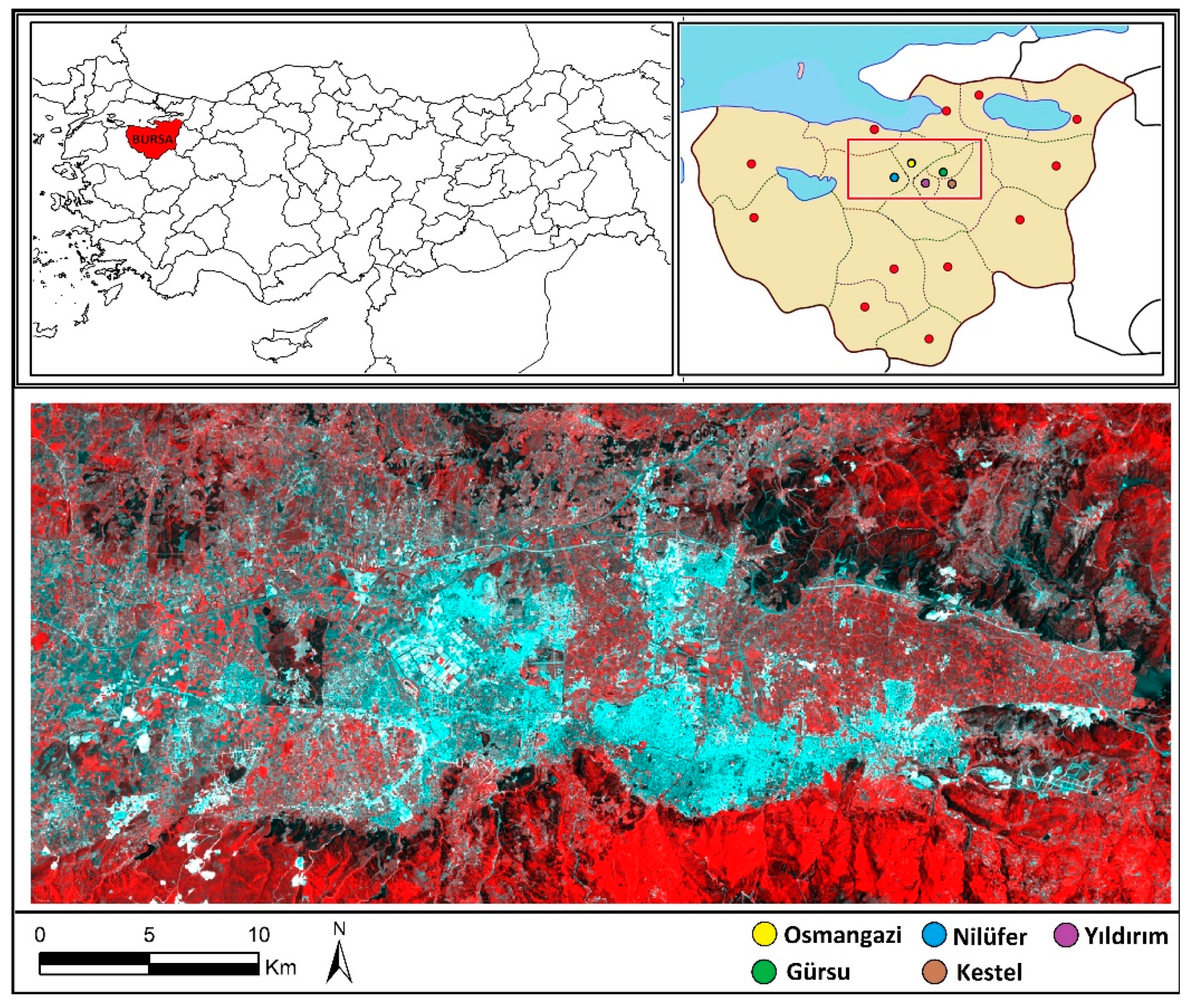
To investigate the SUHI effect of Bursa, Turkey, for 11 time periods from the years 2002 to 2020, multispectral and thermal bands of Landsat images were used. The flowchart of the proposed methodology is shown in Figure 1.

2.1. Study Area

Bursa, which is located in the northwest of Turkey and southeast of the Marmara Sea, is the Turkey’s fourth largest city. According to the Turkish Statistical Institute (TUIK), the 2002 and 2020 populations were 2,231,582 and 3,101,833, respectively [57]. Bursa is situated at an altitude of about 155 m and has a mild climate [58]. However, the climate also varies region by region. In the north, there is a mild and warm climate due to the Marmara Sea, and in the south, there is a harsh climate around the Uludag Mountain. The average annual precipitation is 706 mm, as of the 52-year observation period, and the average relative humidity in the province is around 69% [58]. Bursa is one of the important industrial provinces of Turkey, and there are industrial regions on three urban entrances. In addition, a natural gas combined-cycle power plant is located in the northern part of Bursa province. As a result, Bursa is developing rapidly, and its annual population growth rate was 14.85% for 2019–2020 [57]. Urbanization and industrialization are the most important triggers of the SUHI effect. Therefore, Bursa was chosen as the study area (Figure 2).

2.2. Data Description and Pre-Processing

The only data used in this study were multi-temporal Landsat imageries. MODIS imageries were used for validation. The Landsat images were first obtained in 1972, and Landsat Level-1 data products are used to produce high level scientific data such as surface temperature, water area, snow-covered, and burned areas [59], and they are among the most commonly used images in remote sensing studies because they can be downloaded for free. In this study, Landsat 5 TM and Landsat 8 OLI/TIRS images were used. For the study area, the Landsat images that belonged to the summer season were investigated, and then the July images that had no clouds were selected. At the end, the Landsat 5 TM (16 July 2002, 3 July 2003, 21 July 2004, 30 July 2007, 19 July 2009, 9 July 2011) and Landsat 8 OLI/TIRS (30 July 2013, 20 July 2015, 22 July 2016, 25 July 2017, 1 July 2020) images were downloaded from the USGS Earth Explorer (https://earthexplorer.usgs.gov, accessed on 1 February 2021). Landsat 5 TM images have 6 multispectral and 1 thermal bands, whereas Landsat 8 images have 8 multispectral, 1 panchromatic and 2 thermal bands. For both satellite images, the spatial resolution of the multispectral bands was 30 m. The thermal bands were 120 m and 100 m for Landsat 5 TM and Landsat 8 TIRS, respectively. However, the thermal bands were resampled to 30 m for the delivery products. The Landsat images could be rescaled to the top-of-atmosphere (TOA) reflectance, and the thermal constants (K1 and K2) needed to convert thermal band data to TOA brightness temperature are available in the metadata file [60]. Formulae for these conversions are provided in Section 2.4.

Atmospheric conditions when the images are taken may affect the quality of the LST estimate. Therefore, atmospheric correction was applied to the images. The DOS1 atmospheric correction module of QGIS open-source software was used for this process. This module is based on studies performed by Chavez [61], Sobrino et al. [62], Moran et al. [63] and Congedo [64].

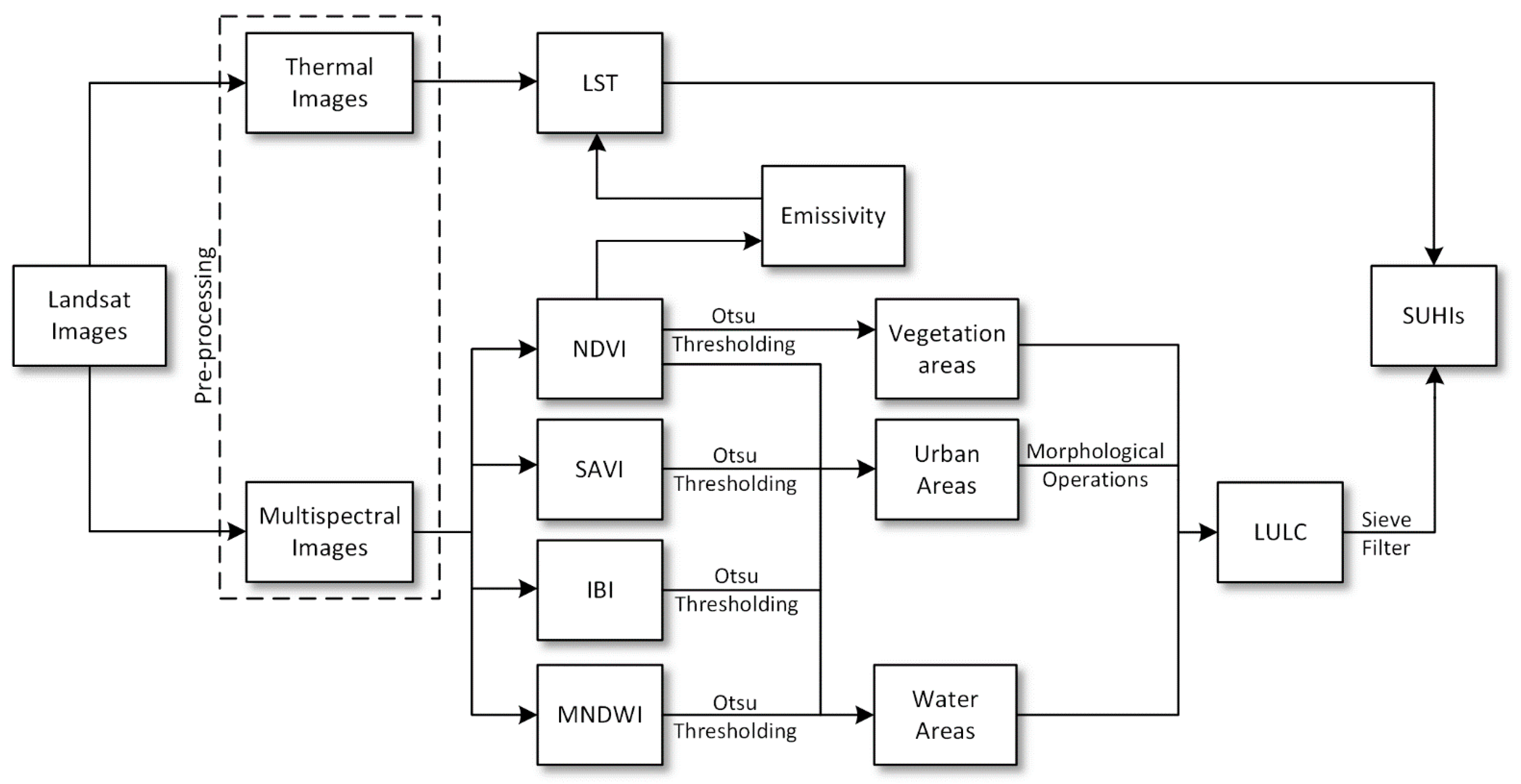
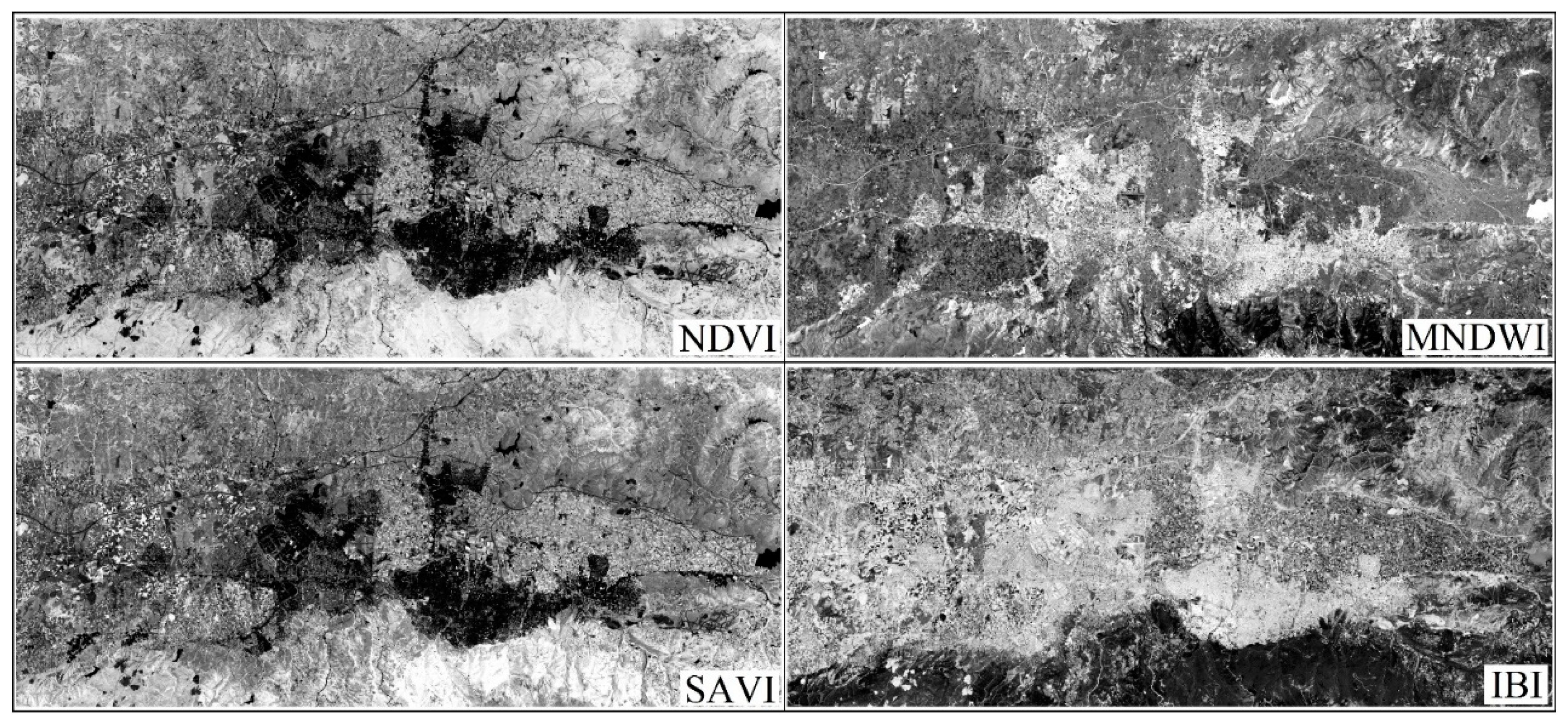
2.3. Generation of Land Cover Indices

Using land cover indices together, different land cover classes can be identified [29,31,49]. In this study NDVI, SAVI, MNDWI, and IBI land cover indices were used. The NDVI is a vegetation index developed by Rouse et al. [65]. SAVI is also a vegetation index, and is used for cities which have an intense urban texture. When compared with the NDVI, the SAVI gives more accurate results for detecting less dense vegetation areas. It is useful for areas that have low vegetation to correct the NDVI for soil brightness influences [66]. The NDVI and SAVI indices are computed using Equations (1) and (2), respectively, and information about vegetation density is presented in the image. The values of these indices vary between –1 and 1. The normalized water difference index was modified (MNDWI) by Xu [67], using GREEN and MIR bands to improve open-water properties (Equation (3)). This modified version reduces built-up land noises that are frequently correlated with open water in other indices. The IBI was proposed by Xu [68] for rapidly built-up area extraction using three thematic indices, NDVI, NDBI and MNDWI. Xu stated that in the IBI image, the built-up areas are enhanced, whereas the background noise is effectively suppressed [68]. In this study, the IBI index was calculated using Equation (4), that enabled the generation of IBI immediately without having to generate the indices [68]. Figure 3 shows the obtained land cover indices for the year 2020.

The formulae for land cover indices used in this study are:

$$\mathrm{NDVI}=\frac{\left(\mathrm{NIR}-\mathrm{RED}\right)}{\left(\mathrm{NIR}+\mathrm{RED}\right)}$$

(1)

$$\mathrm{SAVI}=\frac{\left(\mathrm{NIR}-\mathrm{RED}\right)\left(1+l\right)}{\left(\mathrm{NIR}+\mathrm{RED}+l\right)}$$

(2)

$$\mathrm{MNDWI}=\frac{\left(\mathrm{GREEN}-\mathrm{MIR}\right)}{\left(\mathrm{GREEN}+\mathrm{MIR}\right)}$$

(3)

$$\mathrm{IBI}=\frac{2\mathrm{MIR}/\left(\mathrm{MIR}+\mathrm{NIR}\right)-\left[\mathrm{NIR}/\left(\mathrm{NIR}+\mathrm{RED}\right)+\mathrm{GREEN}/\left(\mathrm{GREEN}+\mathrm{MIR}\right)\right]}{2\mathrm{MIR}/\left(\mathrm{MIR}+\mathrm{NIR}\right)+\left[\mathrm{NIR}/\left(\mathrm{NIR}+\mathrm{RED}\right)+\mathrm{GREEN}/\left(\mathrm{GREEN}+\mathrm{MIR}\right)\right]}$$

(4)

where GREEN is the green band, RED is the red band, NIR is the near-infrared band, MIR is the middle-infrared band, and l is the soil-adjusted correction factor (the value is between 0 and 1: 0 for very dense vegetation; 1 is very sparse vegetation). Generally, this value is accepted as 0.5.

2.4. Obtaining LST Values

Different methods have been developed to estimate LST values. Some of these methods require more than one thermal band (e.g., split window algorithm [27,69,70], multi angle algorithm [71]). However, some methods can be implemented with a single thermal band, e.g., single-channel algorithm [72,73], mono-window algorithm [74,75], and methods that are based on Planck’s law [76,77]. The Landsat 5 TM has one thermal band. Uncertainties were observed in the 11 bands of the Landsat 8 images, and therefore, as the USGS has suggested, users should work with TIRS Band 10 data as a single spectral band [60,75]. Thus, in this study, a method that could be applied with a single thermal band was preferred [76]. The main reason for using this method is that it enables the calculation of LST by utilizing only emissivity values without the need for atmospheric parameters at the time of image acquisition.

Firstly, digital numbers (DN) was converted to radiance using Equation (5):

$${\mathrm{L}}_{\mathrm{b}}=\left({\mathrm{L}}_{\min }+\left({\mathrm{L}}_{\max }-{\mathrm{L}}_{\min }\right)\right)\ast \mathrm{DN}/{\mathrm{Q}}_{\mathrm{CalMax}}$$

(5)

where L_b is the spectral radiance at the top of atmosphere in watts/m²*sr*µm, L_min is the minimum spectral radiance for the thermal band, L_max is the maximum spectral radiance for thermal band, and Q_CalMax represents the maximum quantized and calibrated standard product pixel values (DN).

Brightness temperature was calculated using the spectral radiance with Equation (6):

$${\mathrm{T}}_{\mathrm{B}}=\frac{{\mathrm{K}}_2}{\left(\ln (\frac{{\mathrm{K}}_1}{{\mathrm{L}}_{\mathrm{b}}}+1)\right)}$$

(6)

where T_B is the brightness temperature, and K₁ and K₂ are band-specific thermal conversion constants from the metadata; for Landsat 8 TIRS: K₁ = 774.89 and K₂ = 1321.08, and for Landsat 5 TM: K₁ = 607.76 and K₂ = 1260.56.

Then, the surface temperature (T_S) was derived using Equation (7) [76,77], and it was converted to Celsius (T_C) with Equation (8).

$${\mathrm{T}}_{\mathrm{S}}={\mathrm{T}}_{\mathrm{B}}/(1+\left(ʎ\ast \frac{{\mathrm{T}}_{\mathrm{S}}}{\mathsf{\alpha }}\right)\ast \ln \left(\mathsf{\epsilon }\right)$$

(7)

where ε is the emissivity, ʎ is the average wavelength of the band, and α = 1.438 × 10⁻² mK.

$${\mathrm{T}}_{\mathrm{C}}={\mathrm{T}}_{\mathrm{S}}-273.5$$

(8)

The last step was to derive the calculation emissivity [62,78,79]. Emissivity was calculated with Equation (9):

$${\mathsf{\epsilon }}_{\mathsf{\lambda }}=\{\begin{array}{ll}{\mathsf{\epsilon }}_{\mathrm{s}\mathsf{\lambda }}& \mathrm{NDVI}<{\mathrm{NDVI}}_{\mathrm{s}}\\ {\mathsf{\epsilon }}_{\mathrm{s}\mathsf{\lambda }}+\left({\mathsf{\epsilon }}_{\mathrm{v}\mathsf{\lambda }}-{\mathsf{\epsilon }}_{\mathrm{s}\mathsf{\lambda }}\right)\ast {\mathrm{P}}_{\mathrm{v}}& {\mathrm{NDVI}}_{\mathrm{s}}\le \mathrm{NDVI}\le {\mathrm{NDVI}}_{\mathrm{v}}\\ {\mathsf{\epsilon }}_{\mathrm{v}\mathsf{\lambda }}& \mathrm{NDVI}>{\mathrm{NDVI}}_{\mathrm{v}}\end{array}$$

(9)

where ${\mathsf{\epsilon }}_{\mathsf{\lambda }}$ is the emissivity, ${\mathsf{\epsilon }}_{\mathrm{s}\mathsf{\lambda }}$ is the emissivity value of soil surfaces, ${\mathsf{\epsilon }}_{\mathrm{v}\mathsf{\lambda }}$ is the emissivity value of vegetation surfaces, NDVI_s is the NDVI value of soil surfaces, and NDVI_v is the NDVI value of vegetation surfaces.

The P_v values in Equation (9) can be calculated using Equation (10) [80]:

$${\mathrm{P}}_{\mathrm{v}}={\left[\frac{\mathrm{NDVI}-{\mathrm{NDVI}}_{\mathrm{s}}}{{\mathrm{NDVI}}_{\mathrm{v}}-{\mathrm{NDVI}}_{\mathrm{s}}}\right]}^2$$

(10)

where NDVI_S = 0.2 and NDVI_V = 0.5 [78].

Moreover, in Equation (9), the ε_vλ is 0.99 and the ε_sλ was computed with Equation (11):

$${\mathsf{\epsilon }}_{\mathrm{s}\mathsf{\lambda }}=0.98-0.042\ast \mathrm{RED}$$

(11)

where RED is the red band DN values.

2.5. Extracting Land Cover Areas and Detecting SUHIs

Green plants perform photosynthesis using their chlorophyll pigments. Thus, they use radiation in the red wavelengths of the solar radiation spectrum. Therefore, they absorb a large part of the radiation in the red wavelengths. However, they reflect almost all of the radiation in the near-infrared region. As a result, NDVI shows differentiation between green areas and water surfaces, and gives different values according to the surface properties of the pixels. Hence, it is possible to mention the specific ranges of NDVI values for specific surfaces. If the surface of a pixel contains almost no vegetation in the image, the NDVI value is less than 0.2. When the surface is covered with low-density vegetation texture, the NDVI value ranges between 0.2 and 0.5, whereas when the surface is covered with high-density vegetation, the NDVI value varies between 0.5 and 1 [49,79].

In this study, the threshold values of land cover indices were determined by using the Otsu thresholding method [81]. Then, using these threshold values, urban, vegetation, water and other areas were extracted. For NDVI images, two different threshold values (lower: THR1_NDVI, and higher: THR2_NDVI) were found by using the “multithresh” function of MATLAB R2019a programming language, which is used for determining multilevel image thresholds using Otsu’s method. The vegetation areas were defined from the NDVI images using the higher threshold value (DN_NDVI > THR2_NDVI). On the other hand, for IBI, MNDWI and SAVI images, a single threshold value was computed for each image, again using Otsu’s method. The IBI (DN_IBI > THR_IBI) MNDWI (DN_MNDWI < THR_MNDWI)_, NDVI (DN_NDVI < THR1_NDVI) and SAVI (DN_SAVI < THR_SAVI) images were used to determine urban areas. In addition, water areas were determined using MNDWI images (DN_MNDWI > THR_MNDWI). The conditions and automatically found threshold values which were used to determine the LULC classes in this study are given in

Table 1. The conditions to determine the land cover classes for Landsat 8 OLI images.

Land Cover	Conditions
Urban	DNIBI > THRIBI and DNNDVI < THR1NDVI and DNMNDWI < THRMNDWI and DNSAVI < THRSAVI
Vegetation	DNNDVI > THR2NDVI
Water	DNMNDWI > THRMNDWI

and

Table 2. The obtained threshold values using Otsu’s method for each of the Landsat imageries to determine LULC classes.

Landsat Image Acquisition Date	THR1NDVI–THR2NDVI	THRIBI	THRSAVI	THRMNDWI
16 July 2002	0.14, 0.44	−0.15	0.21	0.16
3 July 2003	0.14, 0.43	−0.15	0.23	0.19
21 July 2004	0.14, 0.44	−0.13	0.21	0.06
30 July 2007	0.13, 0.42	−0.12	0.22	0.08
19 July 2009	0.14, 0.42	−0.13	0.22	0.14
9 July 2011	0.16, 0.47	−0.15	0.23	0.08
30 July 2013	0.12, 0.31	−0.09	0.15	−0.01
20 July 2015	0.13, 0.34	−0.11	0.16	−0.01
22 July 2016	0.12, 0.34	−0.10	0.17	−0.03
25 July 2017	0.12, 0.33	−0.15	0.15	−0.02
1 July 2020	0.21, 0.53	−0.19	0.22	0.12

, respectively.

After obtaining the land cover classes, morphological operations and sieve filters were used as post-processing. Dilation morphological operation was used for the detected urban areas to remove small holes, and the kernel size was determined as 3. Then, the sieve filter was applied to the whole land cover image to remove isolated class pixels.

In this study, the sizes of SUHIs for Bursa were calculated using two methods: (1) SUHI_{Urban–Vegetation}: computing mean LST differences of urban and vegetation areas; (2) SUHI_{Urban–Buffer}: calculating the mean LST differences of urban and surrounding buffer areas. The buffers were generated with 1 km intervals. In this method, four buffer rings were created that had 0—1 km, 1—2 km, 2—3 km, 3—4 km distances from urban areas.

3. Results

The results of this study were examined in three parts: (i) land cover detection; (ii) LST values and variations; and (iii) SUHI detection.

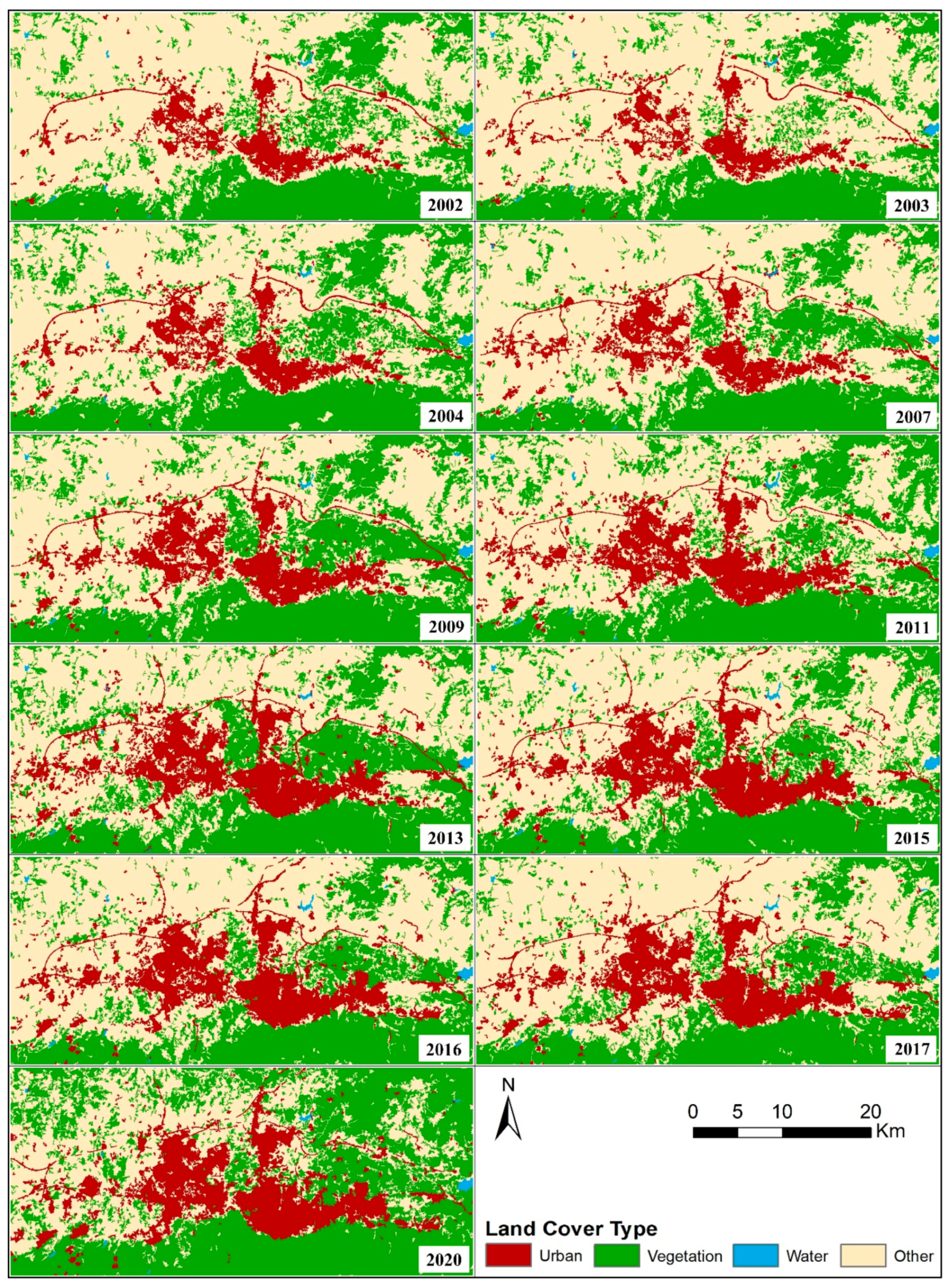
3.1. Land Cover Detection

The obtained land cover images are displayed in Figure 4. To denote the quality and usability of the produced land cover images and to assess the accuracies, test pixels were collected, and error matrices were generated (

Table 3. The obtained producer’s accuracy (PA), user’s accuracy (UA), and overall accuracy values for the years 2002, 2003, 2004, 2007, 2009, 2011, 2013, 2015, 2016, 2017 and 2020.

	Urban		Vegetation		Water		Other
	PA	UA	PA	UA	PA	UA	PA	UA	Overall acc. (%)
2002	0.85	1.00	1.00	0.99	1.00	1.00	0.99	0.87	95.90
2003	0.86	0.94	0.89	0.98	0.98	1.00	0.94	0.79	91.85
2004	0.88	1.00	0.95	0.98	1.00	1.00	0.98	0.85	95.15
2007	0.88	0.95	0.89	0.98	0.94	1.00	0.96	0.78	91.70
2009	0.93	0.91	0.92	0.98	1.00	1.00	0.92	0.88	94.15
2011	0.92	0.83	0.85	0.94	1.00	1.00	0.81	0.82	89.60
2013	0.92	0.78	0.92	0.97	1.00	1.00	0.78	0.87	90.25
2015	0.92	0.92	0.90	0.99	1.00	1.00	0.92	0.85	93.45
2016	0.92	0.81	0.91	1.00	1.00	1.00	0.81	0.85	91.10
2017	0.91	0.87	0.90	0.98	0.95	1.00	0.87	0.79	90.50
2020	0.96	0.81	0.90	0.94	0.95	1.00	0.81	0.88	90.45

). The determination of test pixel size is important during the classification accuracy assessment. Congalton [82] proposed using a minimum of 50 test samples for each land use category and stated that the minimum sample size should be increased to 75 or 100 samples per class if the area is large. Therefore, 500 testing pixels per class were collected in this study.

The land cover areas were successfully identified when the results were analyzed both visually and quantitatively. The overall accuracies were computed as between 89.60% and 95.90% for the 11 time periods between the years 2002 and 2020 (Table 3). These results indicate the quality and usability of the resultant images in SUHI detection studies. When the producer’s and user’s accuracy values were analyzed, it can be stated that the urban, vegetation and water classes which could be used for SUHI computation are quite high. As expected, the water class was determined most accurately, while the vegetation class was the second most accurately determined.

The areas of LULC classes and changes are given in

Table 4. The land cover areas and changes for the years 2002 to 2020.

Image Years	Urban Area (km2)	Vegetation Area (km2)	Water Area (km2)	Other Area (km2)
2002	93.14	383.42	3.23	695.48
2003	96.21	357.65	2.81	718.60
2004	112.21	420.72	3.13	639.21
2007	125.04	361.18	1.79	687.26
2009	151.07	433.81	3.24	587.16
2011	167.24	420.47	3.64	583.91
2013	187.72	423.21	2.76	561.59
2015	183.71	382.51	3.92	605.14
2016	196.13	357.14	3.59	618.41
2017	185.14	350.82	3.01	636.30
2020	210.86	572.44	3.28	388.69
Change 2020–2002 (∆)	117.72	189.02	0.05	−306.79

. For the 18-year time period, it can be observed that the urban and vegetation areas have increased significantly. In contrast, the other areas have decreased considerably. In this time period, the water areas hardly ever changed. The urban areas were found to expand over 93.14 km² in 2002, whereas the extent was 210.86 km² in 2020. The vegetation area was computed as 383.42 km² and 572.44 km² for 2002, and 2020, respectively. On the other hand, the water area was calculated as 3.23 km² for the year 2002 and 3.28 km² for the year 2020. The increases in urban, vegetation and water areas were 117.72 km², 189.02 km² and 0.05 km², respectively, from 2002 to 2020. On the other hand, the decrease in other areas was 306.79 km². These values and visual inspection indicated that, over time, the urban area has expanded into the surrounding areas.

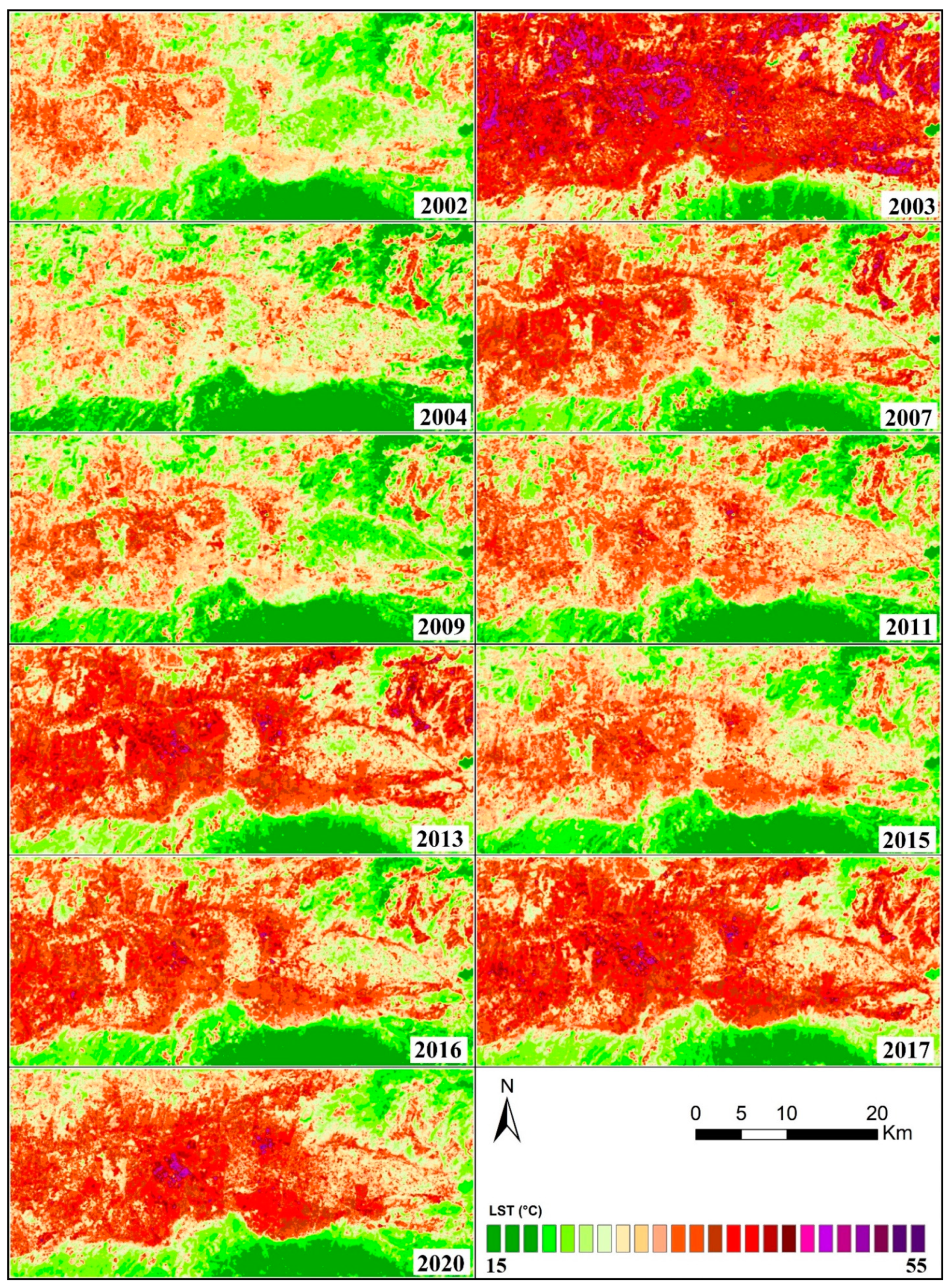
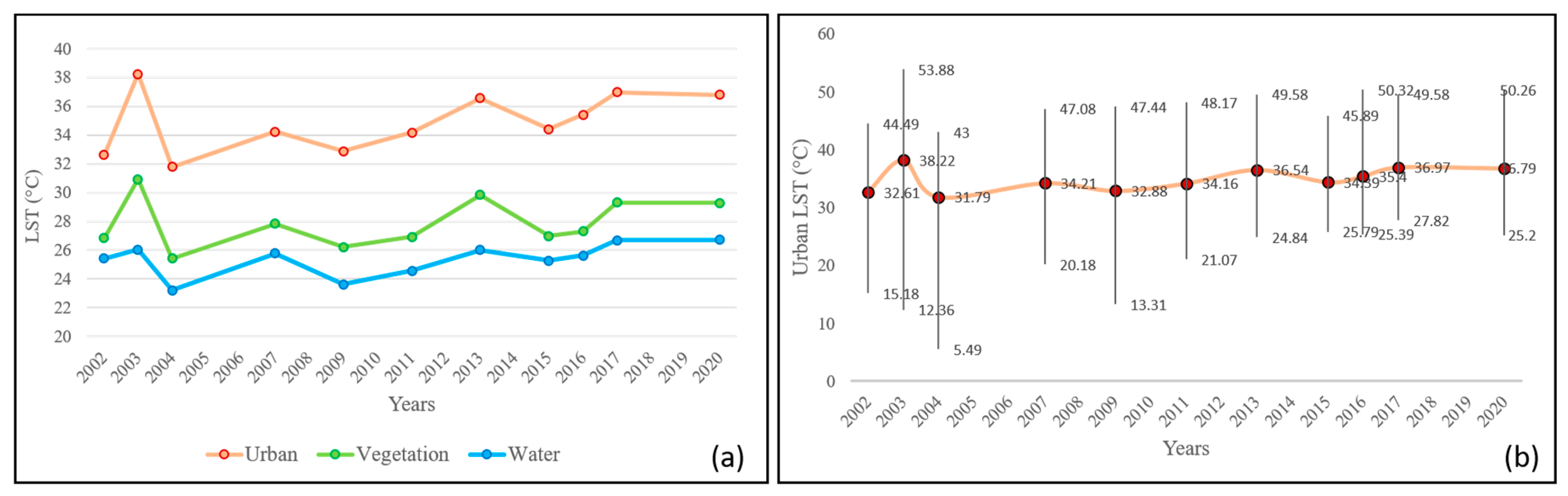
3.2. LST Values and Variations

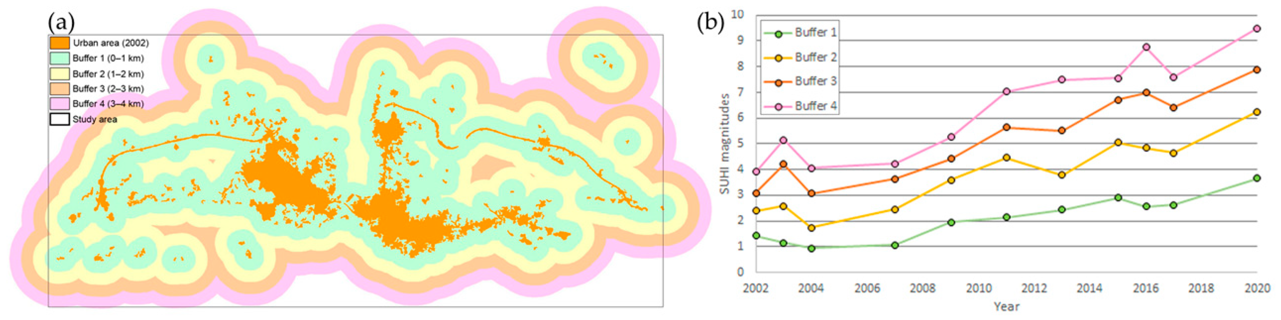
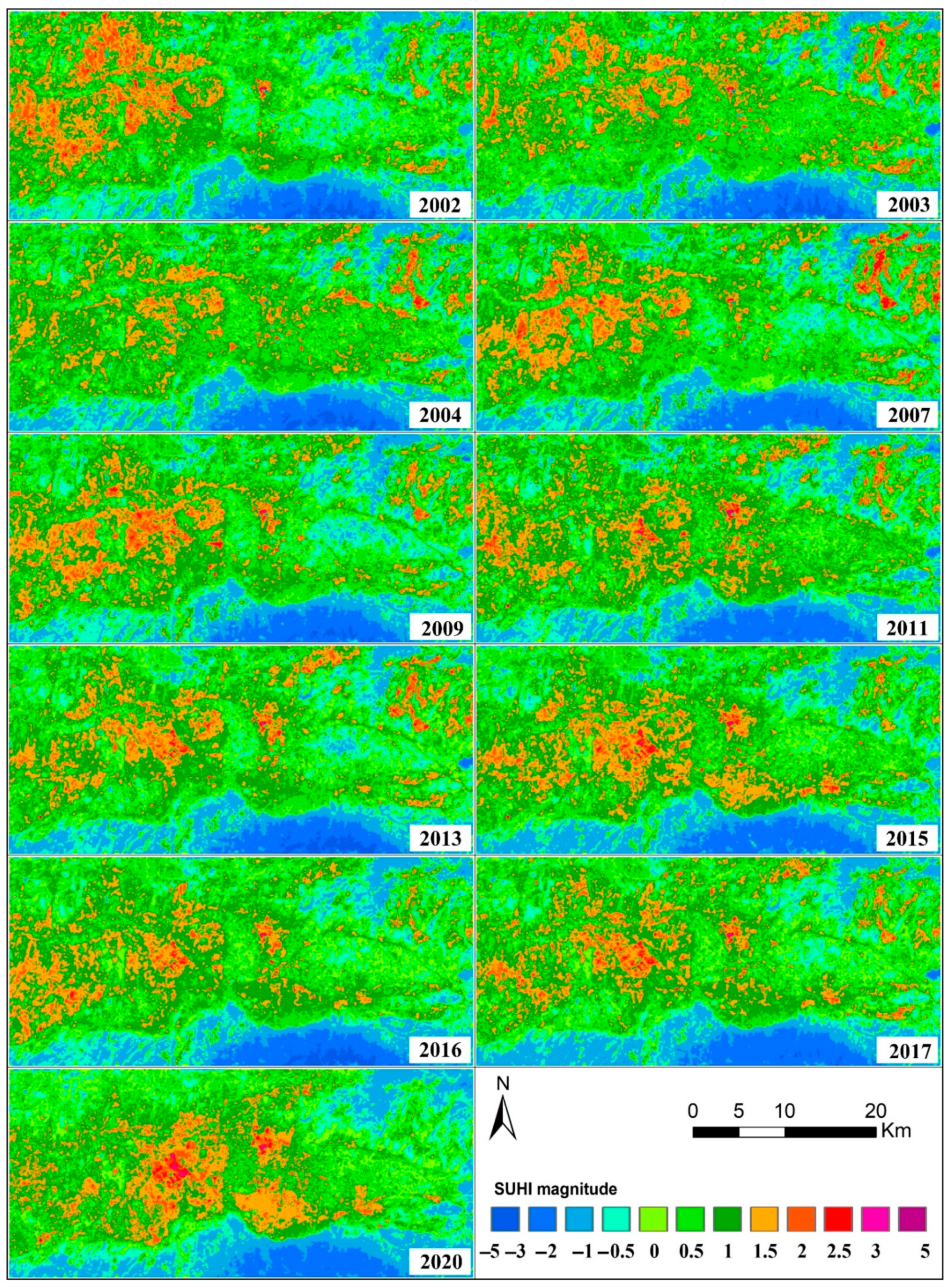
The produced LST images of the study area for 11 time periods from the years 2002 to 2020 are given in Figure 5; the LST graphics that show the mean LST values of urban, vegetation and water classes are given in Figure 6a; for the urban class, minimum, maximum and mean values are given in Figure 6b. When the LST values and maps were analyzed, it can be stated that in general there was an increasing trend for LST values of all classes as well as for the whole study area. However, unexpectedly, there was an extreme increase in 2003, and another unexpected slight increase in 2013.

According to the obtained results, it was observed that Bursa urban areas are warmer than vegetation and water areas in the summer season for all years. The LST values were lowest in water areas, because the daytime images were used. In 2002, the mean LST values of Bursa urban, vegetation and water areas were computed as 32.61 °C, 26.84 °C and 25.42 °C, respectively. In 2020, the mean LST value of the Bursa urban area was computed as 36.79 °C, while LST value of vegetation area was computed as 29.29 °C, and water areas were computed as 26.73 °C. The mean LST values generally increased for urban, vegetation and water areas from 2002 to 2020, and the changes in mean LST values between these years are 4.18 °C for urban areas, 2.45 °C for vegetation areas, and 1.31 °C for water areas. When the urban area was analyzed in detail, it could be seen generally that minimum, maximum and mean LST values increased from 2002 to 2020.

The validity of the obtained LST values was assessed by using MODIS LST/Emissivity data, and the values of MODIS LST were acquired using the (0.02) rescaled factor [83]. The correlation values between the generated Landsat LST and MODIS LST/Emissivity images were calculated using the mean values of the urban, vegetation and water areas. The correlation values were obtained as quite high: 0.89, 0.85, 0.84, 0.94, 0.91, 0.95, 0.97, 0.94, 0.94, 0.95 and 0.94 for 2002, 2003, 2004, 2007, 2009, 2011, 2013, 2015, 2016, 2017 and 2020 images, respectively.

3.3. SUHI Detection

The SUHI values were computed by using mean LST values of urban and vegetation classes and obtained to be 5.77 °C for 2002 and 7.50 °C for 2020 (

Table 5. SUHI magnitude values.

Years	SUHI Magnitudes (°C)
	Buffer 1	Buffer 2	Buffer 3	Buffer 4	Urban–Vegetation
2002	1.43	2.40	3.08	3.91	5.77
2003	1.15	2.59	4.20	5.15	7.30
2004	0.94	1.74	3.07	4.07	6.36
2007	1.07	2.45	3.63	4.22	6.36
2009	1.96	3.59	4.41	5.26	6.66
2011	2.15	4.45	5.65	7.02	7.22
2013	2.44	3.78	5.51	7.49	6.70
2015	2.91	5.04	6.71	7.56	7.40
2016	2.57	4.83	6.98	8.75	8.10
2017	2.63	4.66	6.41	7.60	7.66
2020	3.65	6.26	7.90	9.49	7.50
Change 2020–2002 (∆)	2.22	3.86	4.82	5.58	1.73

). When the changes in the SUHI_{Urban–Vegetation} results were analyzed, there was an important increase over the 18-year time period (1.73 °C).

The SUHI values computed by using mean LST values of urban and buffer areas are given in Table 5. The used buffer areas are shown in Figure 7a, and the graphic that compares SUHIs computed using four buffer areas is given in Figure 7b. The obtained results indicate that, generally, there is an increasing trend in SUHI magnitudes from the years 2002 to 2020. Additionally, it can be stated that the computed SUHI magnitudes increases when the buffer ring area is further away from the urban area, and vice versa. These results can be explained by the possibility that areas farther from the city are more rural, and therefore have lower LST values. For Buffer 1 (0–1 km), Buffer 2 (1–2 km), Buffer 3 (2–3 km) and Buffer 4 (3–4 km), the SUHI magnitudes were computed to be in the ranges of 0.94–3.65, 1.74–6.26, 3.07–7.90 and 3.91–9.49, respectively.

At the end of the study, instead of directly comparing images from different years, the LST was normalized and compared in order to minimize the effect of land use change and different atmospheric conditions between years. SUHI maps were created using normalized LST values using Equation (12). There are studies in the literature which have considered regions with normalized LST values greater than 1.5 °C or greater than 2 °C as SUHI areas [84,85].

$$\mathrm{SUHI}=\left(\mathrm{LST}-\mathrm{LSTmean}\right)/\mathrm{std}$$

(12)

where LST is the pixel LST value, LSTmean is the mean LST of the study area, and std is the standard deviation [85].

When the created SUHI maps were examined, it was seen that the normalized LST values of the urban area increased from 2002 to 2020. The SUHI sizes of some parts of the city and the impermeable surfaces near the city were higher in 2002, whereas SUHI values were higher in the urban area and its immediate surroundings after 2011. The SUHI phenomenon, which was weaker in 2002, strengthened considerably in 2020, and the thermal conditions of the city of Bursa have changed substantially with the growth of the city. It can clearly be seen that the values higher than 1.5 °C correspond to the urban heat island areas in the 2020 SUHI map (Figure 8).

4. Discussion

When the obtained LST values for the whole study area were analyzed, it could be stated that almost all of the LST values increased from the year 2002 to 2020. On the other hand, as can be seen in the LST images (Figure 5) and graphics (Figure 6), the 2003 LST values are extremely high. This situation may give rise to thought that the obtained results are erroneous. However, when the previous temperatures and heat waves were explored, it could be evaluated that the heat wave of 2003 in Europe may have caused these results. The 2003 summer was reported to be the hottest summer since 1500 [86,87,88]. It was said that the sweltering temperatures in summer 2003 had many negative effects, causing the extra deaths of thousands of people [88]. Therefore, according to our evaluation, it is very possible that this heat wave in Europe also affected Bursa. In addition, the 2013 LST values are also relatively high, and it could be because of a 2013 heatwave that affected Europe.

The relationships between LST and IBI and LST and NDVI images for the whole study area were analyzed, and the correlation coefficient values are presented in

Table 6. Correlation coefficient values for LST–IBI and LST–NDVI relationships.

	LST-IBI	LST-NDVI
2002	0.75	−0.75
2003	0.79	−0.76
2004	0.76	−0.72
2007	0.81	−0.77
2009	0.81	−0.78
2011	0.81	−0.78
2013	0.76	−0.69
2015	0.80	−0.74
2016	0.77	−0.71
2017	0.78	−0.73
2020	0.82	−0.80

. The obtained correlation coefficient values indicate that LST presented a strong positive relationship with the IBI image in every situation, with correlation coefficient values higher than 0.75. Conversely, LST and NDVI images had strong negative relationships, and the correlation coefficient values were computed as between –0.69 and –0.80. Guha et al. [89] studied the relationships of NDVI, NDWI, NDBI, and normalized multiband drought index (NMDI) with LST in 11 images from the same year and four different seasons. They found that regardless of the season, LST had negative relationships with NDVI and NMDI, but positive relationships with NDWI and NDBI. These results are similar to our findings.

LST generated using thermal remote sensing techniques is widely used in environmental studies. Although in this study quite high correlation values were found with the produced Landsat LST images and MODIS LST images, it should be noted that there are sources of error (such as error source due to atmospheric effects and emissivity uncertainty) when LST is retrieved from remote sensing data [90].

Although the 2003 LST values were computed to be exceptionally higher than all of the other years, for SUHI magnitudes, the situation was different. The calculated 2003 SUHI magnitudes were higher than the years 2002 and 2004, although lower than other years. This situation reveals that although sudden decreases and rises in temperatures can be observed in some years due to climatic effects, the increase in SUHI effects will continue to increase unless necessary precautions are taken, and the temperature differences between urban and rural areas are increasing.

The obtained SUHI maps show that the highest magnitudes were obtained for urban areas. In this study, residential, industrial and commercial areas were generally defined as urban areas. For detailed information and comparison of different parts of urban areas, zoning was necessary. In Figure 9, the 2020 color-infrared compositions of Landsat imagery and 2020 SUHI map are displayed. Examining these areas more closely with Google Earth images, it could be observed that the SUHI magnitudes of industrial areas had highest values (Figure 9). It was seen that especially Bursa, Demirtas, and Hasanaga organized industrial sites had the highest values.

Considering that SUHI is computed by differencing the mean LST values of urban and rural areas, the correct determination of urban and rural areas in these studies is a very important step that directly affects the results. The classification processes require a lot of time for this stage. The obtained results indicate that with the proposed method used in this study, urban, vegetation and water areas can be obtained quite rapidly and accurately. However, defining rural areas and determining their boundaries is more difficult than urban areas. For this reason, it can be seen that in some studies, the mean LST values of urban–vegetation, urban–water, and urban–non-urban areas are used, whereas in some other studies, urban–buffer areas around the urban area are used. There is no general consent on buffer distances to the urban area. Hence, we used four different buffer rings (0–1 km, 1–2 km, 2–3 km, 3–4 km). The obtained results indicate that the computed SUHI magnitudes were quite different from each other, and the SUHI magnitudes increased when the distance of the buffer ring to the urban area increased. Although the SUHIs were generated by using urban–buffer ring areas, it can be stated that the 3–4 km buffer to the urban area gave the most similar results to SUHIs generated by using the urban–vegetation areas. As a result, the detection of rural areas in SUHI studies is an important issue that should be addressed in future studies. For future work, we are also planning to consider seasonality, using images taken in different seasons.

5. Conclusions

The aims of this study were to determine SUHIs effect easily, efficiently, and rapidly, and to analyze the land cover and land surface temperature (LST) changes, solely using Landsat time series images for 11 time periods from 2002 to 2020. The proposed approach was implemented in Bursa metropolitan city, which is the fourth largest city in Turkey, using the summer season images of the years 2002, 2003, 2004, 2007, 2009, 2011, 2013, 2015, 2016, 2017, 2020; the LULC, LST and SUHI changes were analyzed in this 18-year time period. For this purpose, firstly, the images for these years were obtained, pre-processed, and made suitable for analysis. Then, NDVI, SAVI, MNDWI and IBI indices were produced, and LST data were generated using only Landsat images. Subsequently, the LULC classes were extracted by applying an automatic thresholding technique. Finally, the SUHI magnitudes were calculated using: (i) urban–vegetation LST differences; and (ii) urban–buffer area LST differences.

The LULC detection results were good enough to be used in SUHI extraction purposes, with overall accuracy values between 89.60% and 95.90% for the used images. When the results of the study are examined, it can be seen that the urban area has increased significantly in the 18-year time period. Within this time period, the LST values increased for almost all land cover areas. The obtained LST values indicate that the Bursa metropolitan city is affected by urban warming due to the urbanization process, and probably also by the increase in heatwaves due to climate change. The SUHI magnitudes were computed using urban–vegetation mean LST differences and urban–buffer mean LST differences. The obtained SUHI magnitude values were computed as between 5.77 and 8.10 for the used years when urban–vegetation mean LST differences were used. On the other hand, when urban–buffer mean LST differences were used, the values were computed as between 0.94 and 10.6, and the values increased when the buffer ring area was farther away from the urban area. It was also found that there were significant changes in SUHI magnitudes from 2002 to 2020. Bursa is an industrial city and is developing very rapidly. The obtained results indicate that the urban expansion and LST increase noticeably even in just an 18-year time period, and this situation reveals the importance of considering the climate properties and taking timely precautions during urban planning processes. To mitigate the ongoing increase in the UHI effect over the years, using green/cool roofs, cool pavements, increasing the numbers of trees, and designing efficient landscape areas in urban environments could be solutions.

References

1. United Nations. 2018 Revision of World Urbanization Prospects. Available online: https://www.un.org/development/desa/publications/2018-revision-of-world-urbanization-prospects.html (accessed on 18 January 2021).
2. Estoque, R.C.; Murayama, Y. Measuring Sustainability Based upon Various Perspectives: A Case Study of a Hill Station in Southeast Asia. Ambio 2014, 43, 943–956. [Google Scholar] [CrossRef] [Green Version]
3. Hansen, J.; Sato, M.; Ruedy, R.; Lo, K.; Lea, D.W.; Medina-Elizade, M. Global temperature change. Proc. Natl. Acad. Sci. USA 2006, 103, 14288–14293. [Google Scholar] [CrossRef] [Green Version]
4. Hansen, J.; Ruedy, R.; Sato, M.; Lo, K. Global surface temperature change. Rev. Geophys 2010, 48, RG4004. [Google Scholar] [CrossRef] [Green Version]
5. GISS Goddard Institute for Space Studies. Surface Temperature Analysis (GISTEMP v4). Available online: https://data.giss.nasa.gov/gistemp/ (accessed on 24 June 2019).
6. Feizizadeh, B.; Blaschke, T. Examining Urban heat Island relations to land use and air pollution: Multiple endmember spectral mixture analysis for thermal remote sensing. IEEE J. Sel. Top. Appl. Earth Obs. Remote Sens. 2013, 6, 1749–1756. [Google Scholar] [CrossRef]
7. Mallick, J.; Rahman, A.; Singh, C.K. Modeling urban heat islands in heterogeneous land surface and its correlation with impervious surface area by using night-time ASTER satellite data in highly urbanizing city, Delhi-India. Adv. Sp. Res. 2013, 52, 639–655. [Google Scholar] [CrossRef]
8. Howard, L. Climate of London: Deduced from Metrological Observations, Made in the Metropolis, And at Various Places around It, 3rd ed.; Harvey & Darton: London, UK, 1833. [Google Scholar]
9. Oke, T.R. The energetic basis of the urban heat island. Q. J. R. Meteorol. Soc. 1982, 108, 1–24. [Google Scholar] [CrossRef]
10. Rizwan, A.M.; Dennis, L.Y.C.; Liu, C. A review on the generation, determination and mitigation of Urban Heat Island. J. Environ. Sci. 2008, 20, 120–128. [Google Scholar] [CrossRef]
11. Stewart, I.D.; Oke, T.R. Local climate zones for urban temperature studies. Bull. Am. Meteorol. Soc. 2012, 93, 1879–1900. [Google Scholar] [CrossRef]
12. Deilami, K.; Kamruzzaman, M.; Liu, Y. Urban heat island effect: A systematic review of spatio-temporal factors, data, methods, and mitigation measures. Int. J. Appl. Earth Obs. Geoinf. 2018, 67, 30–42. [Google Scholar] [CrossRef]
13. Zhou, D.; Zhang, L.; Li, D.; Huang, D.; Zhu, C. Climate-vegetation control on the diurnal and seasonal variations of surface urban heat islands in China. Environ. Res. Lett. 2016, 11, 074009. [Google Scholar] [CrossRef]
14. Bornstein, R.D. Observations of the Urban Heat Island Effect in New York City. J. Appl. Meteorol. 1968, 7, 575–582. [Google Scholar] [CrossRef]
15. Kolokotroni, M.; Giannitsaris, I.; Watkins, R. The effect of the London urban heat island on building summer cooling demand and night ventilation strategies. Sol. Energy 2006, 80, 383–392. [Google Scholar] [CrossRef]
16. Peterson, T.C. Assessment of urban versus rural in situ surface temperatures in the contiguous United States: No difference found. J. Clim. 2003, 16, 2941–2959. [Google Scholar] [CrossRef] [Green Version]
17. Sun, R.; Lü, Y.; Yang, X.; Chen, L. Understanding the variability of urban heat islands from local background climate and urbanization. J. Clean. Prod. 2019, 208, 743–752. [Google Scholar] [CrossRef]
18. Vardoulakis, E.; Karamanis, D.; Fotiadi, A.; Mihalakakou, G. The urban heat island effect in a small Mediterranean city of high summer temperatures and cooling energy demands. Sol. Energy 2013, 94, 128–144. [Google Scholar] [CrossRef]
19. Aniello, C.; Morgan, K.; Busbey, A.; Newland, L. Mapping micro-urban heat islands using LANDSAT TM and a GIS. Comput. Geosci. 1995, 21, 965–967, 969. [Google Scholar] [CrossRef]
20. Carnahan, W.H.; Larson, R.C. An Analysis of an Urban Heat Sink. Remote Sens. Environ. 1990, 33, 65–71. [Google Scholar] [CrossRef]
21. Voogt, J.A.; Oke, T.R. Thermal remote sensing of urban climates. Remote Sens. Environ. 2003, 86, 370–384. [Google Scholar] [CrossRef]
22. Feng, H.; Zhao, X.; Chen, F.; Wu, L. Using land use change trajectories to quantify the effects of urbanization on urban heat island. Adv. Sp. Res. 2014, 53, 463–473. [Google Scholar] [CrossRef]
23. Geletič, J.; Lehnert, M.; Savić, S.; Milošević, D. Inter-/intra-zonal seasonal variability of the surface urban heat island based on local climate zones in three central European cities. Build. Environ. 2019, 156, 21–32. [Google Scholar] [CrossRef]
24. Hung, T.; Daisuke, U.; Shiro, O.; Yoshifumi, Y. Assessment with satellite data of the urban heat island effects in Asian mega cities. Int. J. Appl. Earth Obs. Geoinf. 2006, 8, 34–48. [Google Scholar] [CrossRef]
25. Rao, P.K. Remote sensing of urban “heat islands” from an environmental satellite. Bull. Am. Meteorol. Soc. 1972, 53, 647–648. [Google Scholar]
26. Alves, E.D.L. Seasonal and spatial variation of surface urban heat island intensity in a small urban agglomerate in Brazil. Climate 2016, 4, 61. [Google Scholar] [CrossRef] [Green Version]
27. Jin, M.; Li, J.; Wang, C.; Shang, R. A practical split-window algorithm for retrieving land surface temperature from Landsat-8 data and a case study of an urban area in China. Remote Sens. 2015, 7, 4371–4390. [Google Scholar] [CrossRef] [Green Version]
28. Parastatidis, D.; Mitraka, Z.; Chrysoulakis, N.; Abrams, M. Online global land surface temperature estimation from landsat. Remote Sens. 2017, 9, 1208. [Google Scholar] [CrossRef] [Green Version]
29. Ranagalage, M.; Estoque, R.C.; Murayama, Y. An urban heat island study of the Colombo Metropolitan Area, Sri Lanka, based on Landsat data (1997–2017). ISPRS Int. J. Geo-Inf. 2017, 6, 189. [Google Scholar] [CrossRef] [Green Version]
30. Lang, Q.; Yu, W.; Ma, M.; Wen, J. Analysis of the spatial and temporal evolution of land cover and heat island effects in six districts of Chongqing’s main city. Sensors 2019, 19, 5239. [Google Scholar] [CrossRef] [Green Version]
31. Chen, X.L.; Zhao, H.M.; Li, P.X.; Yin, Z.Y. Remote sensing image-based analysis of the relationship between urban heat island and land use/cover changes. Remote Sens. Environ. 2006, 104, 133–146. [Google Scholar] [CrossRef]
32. Haashemi, S.; Weng, Q.; Darvishi, A.; Alavipanah, S.K. Seasonal variations of the surface urban heat Island in a semi-arid city. Remote Sens. 2016, 8, 352. [Google Scholar] [CrossRef] [Green Version]
33. Li, J.-J.; Wang, X.-R.; Wang, X.-J.; Ma, W.-C.; Zhang, H. Remote sensing evaluation of urban heat island and its spatial pattern of the Shanghai metropolitan area, China. Ecol. Complex. 2009, 6, 413–420. [Google Scholar] [CrossRef]
34. Pal, S.; Ziaul, S. Detection of land use and land cover change and land surface temperature in English Bazar urban centre. Egypt. J. Remote Sens. Sp. Sci. 2017, 20, 125–145. [Google Scholar] [CrossRef] [Green Version]
35. Singh, P.; Kikon, N.; Verma, P. Impact of land use change and urbanization on urban heat island in Lucknow city, Central India. A remote sensing based estimate. Sustain. Cities Soc. 2017, 32, 100–114. [Google Scholar] [CrossRef]
36. Kamali Maskooni, E.; Hashemi, H.; Berndtsson, R.; Daneshkar Arasteh, P.; Kazemi, M. Impact of spatiotemporal land-use and land-cover changes on surface urban heat islands in a semiarid region using Landsat data. Int. J. Digit. Earth 2021, 14, 250–270. [Google Scholar] [CrossRef]
37. Geletič, J.; Lehnert, M.; Dobrovolný, P. Land surface temperature differences within local climate zones, based on two central European cities. Remote Sens. 2016, 8, 788. [Google Scholar] [CrossRef] [Green Version]
38. Mathew, A.; Khandelwal, S.; Kaul, N. Investigating spatial and seasonal variations of urban heat island effect over Jaipur city and its relationship with vegetation, urbanization and elevation parameters. Sustain. Cities Soc. 2017, 35, 157–177. [Google Scholar] [CrossRef]
39. Streutker, D.R. A remote sensing study of the urban heat island of Houston, Texas. Int. J. Remote Sens. 2002, 23, 2595–2608. [Google Scholar] [CrossRef]
40. Zhao, M.; Cai, H.; Qiao, Z.; Xu, X. Influence of urban expansion on the urban heat island effect in Shanghai. Int. J. Geogr. Inf. Sci. 2016, 30, 2421–2441. [Google Scholar] [CrossRef]
41. Chen, W.; Zhang, Y.; Pengwang, C.; Gao, W. Evaluation of urbanization dynamics and its impacts on surface heat islands: A case study of Beijing, China. Remote Sens. 2017, 9, 453. [Google Scholar] [CrossRef] [Green Version]
42. Gallo, K.P.; McNab, A.L.; Karl, T.R.; Brown, J.F.; Hood, J.J.; Tarpley, J.D. The use of a vegetation index for assessment of the urban heat island effect. Int. J. Remote Sens. 1993, 14, 2223–2230. [Google Scholar] [CrossRef]
43. Zhou, W.; Qian, Y.; Li, X.; Li, W.; Han, L. Relationships between land cover and the surface urban heat island: Seasonal variability and effects of spatial and thematic resolution of land cover data on predicting land surface temperatures. Landsc. Ecol. 2014, 29, 153–167. [Google Scholar] [CrossRef]
44. Estoque, R.C.; Murayama, Y.; Myint, S.W. Effects of landscape composition and pattern on land surface temperature: An urban heat island study in the megacities of Southeast Asia. Sci. Total Environ. 2017, 577, 349–359. [Google Scholar] [CrossRef]
45. Kumar, D.; Shekhar, S. Statistical analysis of land surface temperature-vegetation indexes relationship through thermal remote sensing. Ecotoxicol. Environ. Saf. 2015, 121, 39–44. [Google Scholar] [CrossRef]
46. Gallo, K.P.; McNab, A.L.; Karl, T.R.; Brown, J.F.; Hood, J.J.; Tarpley, J.D. The Use of NOAA AVHRR Data for Assessment of the Urban Heat-Island Effect. J. Appl. Meteorol. Climatol. 1993, 32, 899–908. [Google Scholar] [CrossRef] [Green Version]
47. Gallo, K.P.; Tarpley, J.D.; McNab, A.L.; Karl, T.R. Assessment of urban heat islands: A satellite perspective. Atmos. Res. 1995, 37, 37–43. [Google Scholar] [CrossRef]
48. Zhang, Y.; Odeh, I.O.A.; Han, C. Bi-temporal characterization of land surface temperature in relation to impervious surface area, NDVI and NDBI, using a sub-pixel image analysis. Int. J. Appl. Earth Obs. Geoinf. 2009, 11, 256–264. [Google Scholar] [CrossRef]
49. Guha, S.; Govil, H.; Dey, A.; Gill, N. Analytical study of land surface temperature with NDVI and NDBI using Landsat 8 OLI and TIRS data in Florence and Naples city, Italy. Eur. J. Remote Sens. 2018, 51, 667–678. [Google Scholar] [CrossRef]
50. Lemus-Canovas, M.; Martin-Vide, J.; Moreno-Garcia, M.C.; Lopez-Bustins, J.A. Estimating Barcelona’s metropolitan daytime hot and cold poles using Landsat-8 Land Surface Temperature. Sci. Total Environ. 2020, 699, 134307. [Google Scholar] [CrossRef] [PubMed]
51. Muzaky, H.; Jaelani, L.M. Analysis of the impact of land cover on Surface Temperature Distribution: Urban heat island studies i}n Medan and Makassar. IOP Conf. Ser. Earth Environ. Sci. 2019, 389, 012047. [Google Scholar] [CrossRef]
52. Sekertekin, A.; Zadbagher, E. Simulation of future land surface temperature distribution and evaluating surface urban heat island based on impervious surface area. Ecol. Indic. 2021, 122, 107230. [Google Scholar] [CrossRef]
53. Li, K.; Chen, Y.; Wang, M.; Gong, A. Spatial-temporal variations of surface urban heat island intensity induced by different definitions of rural extents in China. Sci. Total Environ. 2019, 669, 229–247. [Google Scholar] [CrossRef] [PubMed]
54. Wu, X.; Wang, G.; Yao, R.; Wang, L.; Yu, D.; Gui, X. Investigating surface urban heat islands in South America based on MODIS data from 2003–2016. Remote Sens. 2019, 11, 1212. [Google Scholar] [CrossRef] [Green Version]
55. Yao, R.; Wang, L.; Huang, X.; Niu, Z.; Liu, F.; Wang, Q. Temporal trends of surface urban heat islands and associated determinants in major Chinese cities. Sci. Total Environ. 2017, 609, 742–754. [Google Scholar] [CrossRef]
56. Zhou, D.; Zhao, S.; Liu, S.; Zhang, L.; Zhu, C. Surface urban heat island in China’s 32 major cities: Spatial patterns and drivers. Remote Sens. Environ. 2014, 152, 51–61. [Google Scholar] [CrossRef]
57. TUIK Turkish Statistical Institute. Available online: http://www.tuik.gov.tr/UstMenu.do?metod=temelist (accessed on 20 June 2019).
58. Bursa’s Geography/Climate/Population. Available online: http://www.bursa.com.tr/bursas-geography-climate-population?lang=en (accessed on 18 January 2021).
59. USGS Landsat Missions Product Information. Available online: https://www.usgs.gov/land-resources/nli/landsat/product-information (accessed on 18 January 2021).
60. USGS Landsat 8 (L8) Data Users Handbook, v4. 106p. Available online: https://www.usgs.gov/land-resources/nli/landsat/landsat-8-data-users-handbook (accessed on 24 June 2019).
61. Chavez, P.S. Image-Based Atmospheric Corrections—Revisited and Improved Photogrammetric Engineering and Remote Sensing. Am. Soc. Photogramm. 1996, 62, 1025–1036. [Google Scholar]
62. Sobrino, J.A.; Jiménez-Muñoz, J.C.; Paolini, L. Land surface temperature retrieval from LANDSAT TM 5. Remote Sens. Environ. 2004, 90, 434–440. [Google Scholar] [CrossRef]
63. Moran, M.S.; Jackson, R.D.; Slater, P.N.; Teillet, P.M. Evaluation of simplified procedures for retrieval of land surface reflectance factors from satellite sensor output. Remote Sens. Environ. 1992, 41, 169–184. [Google Scholar] [CrossRef]
64. Congedo, L. Semi-Automatic Classification Plugin Documentation. Release 5.3.2.1. Available online: https://media.readthedocs.org/pdf/semiautomaticclassificationmanual-v4/latest/semiautomaticclassificationmanual-v4.pdf (accessed on 24 June 2019).
65. Rouse, J.W.; Haas, R.H.; Schell, J.A.; Deering, D.W. Monitoring Vegetation Systems in the Great Plains with ERTS. In Proceedings of the Third Earth Resources Technology Satellite-1 Symposium, Greenbelt, MD, USA, 10–14 December 1973. NASA SP-351 Series. [Google Scholar]
66. Huete, A.R. A Soil-adjusted Vegetation Index (SAVI). Remote Sens. Environ. 1988, 25, 295–309. [Google Scholar] [CrossRef]
67. Xu, H. Modification of normalised difference water index (NDWI) to enhance open water features in remotely sensed imagery. Int. J. Remote Sens. 2006, 27, 3025–3033. [Google Scholar] [CrossRef]
68. Xu, H. A new index for delineating built-up land features in satellite imagery. Int. J. Remote Sens. 2008, 29, 4269–4276. [Google Scholar] [CrossRef]
69. Du, C.; Ren, H.; Qin, Q.; Meng, J.; Li, J. Split-Window Algorithm for Estimating Land Surface Temperature from Landsat 8 Tirs Data. In Proceedings of the 2014 IEEE Geoscience and Remote Sensing Symposium (IGARSS), Quebec City, QC, Canada, 13–18 July 2014; IEEE: Piscataway, NJ, USA, 2014; pp. 3578–3581, ISBN 978-1-4799-5775-0. [Google Scholar]
70. Sobrino, J.A.; Caselles, V.; Coll, C. Theoretical split-window algorithms for determining the actual surface temperature. Nuovo Cim. C 1993, 16, 219–236. [Google Scholar] [CrossRef]
71. Zhaoliang, L.; Stoll, M.P.; Renhua, Z.; Li, J.; Su, Z. On the separate retrieval of soil and vegetation temperatures from ATSR data. Sci. China Ser. D Earth Sci. 2001, 44, 97–111. [Google Scholar] [CrossRef]
72. Yu, X.; Guo, X.; Wu, Z. Land surface temperature retrieval from landsat 8 TIRS-comparison between radiative transfer equation-based method, split window algorithm and single channel method. Remote Sens. 2014, 6, 9829–9852. [Google Scholar] [CrossRef] [Green Version]
73. Jiménez-Munoz, J.C.; Sobrino, J.A. A generalized single-channel method for retrieving land surface temperature from remote sensing data. J. Geophys. Res. D Atmos. 2003, 108, 4688. [Google Scholar] [CrossRef] [Green Version]
74. Qin, Z.; Karnieli, A.; Berliner, P. A mono-window algorithm for retrieving land surface temperature from Landsat TM data and its application to the Israel-Egypt border region. Int. J. Remote Sens. 2001, 22, 3719–3746. [Google Scholar] [CrossRef]
75. Wang, F.; Qin, Z.; Song, C.; Tu, L.; Karnieli, A.; Zhao, S. An improved mono-window algorithm for land surface temperature retrieval from landsat 8 thermal infrared sensor data. Remote Sens. 2015, 7, 4268–4289. [Google Scholar] [CrossRef] [Green Version]
76. Artis, D.A.; Carnahan, W.H. Survey of emissivity variability in thermography of urban areas. Remote Sens. Environ. 1982, 12, 313–329. [Google Scholar] [CrossRef]
77. Weng, Q.; Lu, D.; Schubring, J. Estimation of land surface temperature-vegetation abundance relationship for urban heat island studies. Remote Sens. Environ. 2004, 89, 467–483. [Google Scholar] [CrossRef]
78. Sobrino, J.A.; Jiménez-Muñoz, J.C.; Sòria, G.; Romaguera, M.; Guanter, L.; Moreno, J.; Plaza, A.; Martínez, P. Land surface emissivity retrieval from different VNIR and TIR sensors. IEEE Trans. Geosci. Remote Sens. 2008, 46, 316–327. [Google Scholar] [CrossRef]
79. Sobrino, J.A.; Raissouni, N. Toward remote sensing methods for land cover dynamic monitoring: Application to Morocco. Int. J. Remote Sens. 2000, 21, 353–366. [Google Scholar] [CrossRef]
80. Carlson, T.N.; Ripley, D.A. On the relation between NDVI, fractional vegetation cover, and leaf area index. Remote Sens. Environ. 1997, 62, 241–252. [Google Scholar] [CrossRef]
81. Otsu, N. A Threshold Selection Method from Gray-Level Histograms. IEEE Trans. Syst. Man Cybern. 1979, 9, 62–66. [Google Scholar] [CrossRef] [Green Version]
82. Congalton, R.G. A review of assessing the accuracy of classifications of remotely sensed data. Remote Sens. Environ. 1991, 37, 35–46. [Google Scholar] [CrossRef]
83. Wan, Z. Collection-6 MODIS Land Surface Temperature Products Users’ Guide. Available online: https://lpdaac.usgs.gov/documents/118/MOD11_User_Guide_V6.pdf (accessed on 18 January 2021).
84. Ahmed, S. Assessment of urban heat islands and impact of climate change on socioeconomic over Suez Governorate using remote sensing and GIS techniques. Egypt. J. Remote Sens. Sp. Sci. 2018, 21, 15–25. [Google Scholar] [CrossRef]
85. Abutaleb, K.; Ngie, A.; Darwish, A.; Ahmed, M.; Arafat, S.; Ahmed, F. Assessment of Urban Heat Island Using Remotely Sensed Imagery over Greater Cairo, Egypt. Adv. Remote Sens. 2015, 4, 35–47. [Google Scholar] [CrossRef] [Green Version]
86. Luterbacher, J.; Dietrich, D.; Xoplaki, E.; Grosjean, M.; Wanner, H. European Seasonal and Annual Temperature Variability, Trends, and Extremes since 1500. Science 2004, 303, 1499–1503. [Google Scholar] [CrossRef] [Green Version]
87. Stott, P.; Stone, D.; Allen, M. Human contribution to the European heatwave of 2003. Nature 2004, 432, 610–614. [Google Scholar] [CrossRef]
88. Khamsi, R. Human activity implicated in Europe’s 2003 heat wave. Nature 2004. [Google Scholar] [CrossRef]
89. Guha, S.; Govil, H.; Diwan, P. Analytical study of seasonal variability in land surface temperature with normalized difference vegetation index, normalized difference water index, normalized difference built-up index, and normalized multiband drought index. J. Appl. Remote Sens. 2019, 13, 024518. [Google Scholar] [CrossRef] [Green Version]
90. Jiménez-Muñoz, J.C.; Sobrino, J.A. Error sources on the land surface temperature retrieved from thermal infrared single channel remote sensing data. Int. J. Remote Sens. 2006, 27, 999–1014. [Google Scholar] [CrossRef]
Figure 1. The flowchart of the overall processes.
Ijgi 10 00416 g001
Figure 2. The color infrared Landsat 8 OLI imagery (2020) of the study area and its location in Turkey and Bursa.
Ijgi 10 00416 g002
Figure 3. The obtained NDVI, SAVI, MNDWI and IBI remote sensing indices using the Landsat 8 image obtained on 1 July 2020.
Ijgi 10 00416 g003
Figure 4. The obtained land cover classes using the index-based method for the years 2002, 2003, 2004, 2007, 2009, 2011,2013, 2015, 2016, 2017 and 2020.
Ijgi 10 00416 g004
Figure 5. LST imagery of the study area for the years: 2002, 2003, 2004, 2007, 2009, 2011, 2013, 2015, 2016, 2017 and 2020.
Ijgi 10 00416 g005
Figure 6. The mean LST values of urban, vegetation and water land cover areas (a), and minimum, maximum and mean LST values of urban areas (b).
Ijgi 10 00416 g006
Figure 7. The 2002 urban area and buffer rings with 1 km intervals (a) and the buffer SUHI magnitudes between the years 2002 and 2020 (b).
Ijgi 10 00416 g007
Figure 8. The UHI maps of the study area for the years: 2002, 2003, 2004, 2007, 2009, 2011, 2013, 2015, 2016, 2017 and 2020.
Ijgi 10 00416 g008
Figure 9. The Google Earth image and SUHI map of the areas shown in the false color Landsat image (2020) and SUHI map of the study area: 1. Bursa organized industrial site; 2. Nilufer small industrial site; 3. Hasanaga organized industrial site; 4. Demirtas organized industrial site; 5. Kestel organized industrial site.
Ijgi 10 00416 g009