DEM-Based UAV Flight Planning for 3D Mapping of Geosites: The Case of Olympus Tectonic Window, Lesvos, Greece

Abstract

Geosites are an important part of geoheritage, thus their detailed mapping is crucial for their management, protection and promotion processes. However, there is no specific approach to three-dimensional (3D) mapping of geosites and a full investigation is required, considering the current advances in the science of Geoinformatics and the need for setting up an integrated system that will suggest a suitable way of mapping areas of geological significance. The main purpose of this study is to explore new approaches to the 3D mapping of geosites, where the unmanned aerial vehicles’ (UAVs) flight planning is based on the digital elevation model (DEM). The case study that is being examined is the tectonic window of Mount Olympus, located in the southeast of Lesvos island, Greece. In this paper, a methodology has been developed to create flight plans for geosite 3D mapping. This methodology consists of three main stages: (a) flight planning based on SRTM-DEM, (b) data acquisition and image-based 3D modelling, and (c) comparison (flight plans and results). A semi-automated algorithm was developed for designing the flights, taking into account the topography of the mapped area (slope, aspect, elevation) and the final cartographic derivatives. The flight plans were compared with each other in levels of data collection, flight characteristics and their results. The results of this study are dense point clouds, DEMs and orthophotomaps. The algorithms that have been used for the comparison of point clouds were (I) surface density, (II) number of neighbours (NN), and (III) roughness and surface profile. The conclusion drawn from this study is that the DEM is a valuable source of information that can be used in designing flight plans specially shaped on the topography of each geosite.

1. Introduction

Geoheritage is part of natural heritage. It includes a variety of geosites, that can be wider landscapes, single landforms or rock assemblages, that represent important events from Earth’s history, the evolution of life or active geodynamic processes. Geosites consist of elements of high scientific, educational and tourist value, worth securing for the following generations. All geographical arrangements and elements aid in the study of (a) the formation and evolution of the Earth, (b) its conditions and situations over time, and (c) the beginning and evolution of life. As per Brocx and Semeniuk (2007) [1], geoheritage (topographical legacy) is concerned with the protection of highlights important for Earth science, for example landforms, excavations, exposures and locales where geographical highlights can be analyzed. Recently, mapping has gained greater value in geoheritage research [2,3]. Geoheritage mapping is important in managing and protecting natural areas, being essential to the territory’s prescriptive zoning [4]. A geosite constitutes part of the geoheritage of a territory [5]. Geosites are spatially specific sections of geological and geomorphological significance [6] and have been considered worthy of protection in understanding the history of the Earth. Geosites are important elements for measuring geodiversity and geoheritage, thus detailed mapping is crucial for their management, protection and promotion. Combined with technologies such as geographical information systems (GIS), traditional geological mapping acquired a digital character [7] and expanded into three dimensions [8]. 3D mapping detects mid-high slope transformation characterized by large fractured rock masses and can provide scientific information on a geosite before it is affected by the activation of the instability phenomena [2].

In previous years, 3D mapping of geological structures was done by topographic methods, remote sensing, GIS software and digital globes like Google Earth and NASA’s World Wind [9,10]. However, the development of new digital technologies and geoinformatics have influenced geo-heritage scientific practices. In recent years, the use of unmanned aerial vehicles (UAVs) has been incorporated into the science of Geoinformatics, offering the ability to map areas in 3D, while accurately providing geospatial data in ultra-high resolution [11,12]. Structure-from-Motion (SfM) and multi-view stereo (MVS) algorithms [13,14] that can be applied to images taken by cameras mounted on UAVs, have become significant as a new way of generating high resolution topography [15]. Three-dimensional mapping has been applied to different geological structures such as granite rock [16], gorge [17], landslides [18], caves [19] and lava flows [20]. A series of recent studies has shown that the UAV photogrammetry and the quality information it offers can be applied to rapid mapping and geomorphological surveys [21,22,23]. Several studies have suggested that the UAV’s data acquisition for geomorphological fluctuation can be fast, accurate and low-cost in obtaining multi-temporal topographical information, particularly for geomorphological analysis [14,18,24,25]. In addition, the evolution of geovisualization tools has allowed the synergistic utilization of technologies such as virtual (VR) and augmented reality (AR) in UAV data visualization in virtual environments. The specific media achieved the communication of the geographical information with the user, using modern and interactive methods. Through VR and AR, the promotion and management of geological structures and geosites acquired a dynamic character, as it became possible to monitor and visit those areas worldwide using these specific techniques [26]. A very important parameter is the transferring of the 3D geographic information into a virtual space, as it demands the produced cartographic result to be accurate and in high resolution [27,28]. In order to evaluate the accuracy of a point cloud derived from UAV-photogrammetry, authors compare it with a terrestrial laser scanner or LiDAR data [26,27,28,29]. It is also suggested that even a commercial UAV can yield data suitable for measuring geomorphic changes [18]. The automatically pre-designed photogrammetric planning and control of UAV flights plays an essential role in providing quality images and thus good cartographic results. The quality of a 3D model depends on flight planning characteristics, such as the geometrical parameters of: (I) ground sampling distance (GSD) and (II) front and side overlap, and the UAV’s flight parameters, which consist of (I) the angle of the camera, (II) the height of the flight, (III) the orientation of the aircraft and (IV) the path that the UAV follows [30,31,32].

A very important factor in creating a flight plan is the path that the UAV will follow, as its course determines the orientation of the camera which in turn defines the aspect that is going to be captured [33]. Therefore, it will not be possible to capture a gap that might exist to the opposite of the camera angle. In recent years, the trajectory of a UAV flying at a steady height and with constant front and side overlap in a cross grid, polygon or circular pattern has been established as an efficient data collection pattern [34,35]. However, this flight path was not always efficient in high relief landscapes, sharp slopes and composite surfaces [36]. The high relief negatively affects the photograph’s scale and GSD, which changed dramatically when the UAV flew at a constant height, as in reality the photographs did not depict information with the same spatial analysis when capturing a high-altitude area. To deal with this problem, there were surveys where the camera was placed vertically to the ground, following a constant course over the terrain [36,37]. Limitations also appeared in this particular methodology, as from the DEM, only the elevation value is used, while the aspect and the slope were not taken into account. As a result, the steep slopes could not be identified. A different way of obtaining aerial images of inclined or composite surfaces is the collection of both oblique photos and a fusion of oblique and vertical photos [16,38,39,40], acquired from manual flights or post-flight processes that combine data from flights with different trajectories. Despite the fact that there are lots of available flight planning applications that effectively allow terrain following based on DEM information for terrain awareness purposes, there is not an available application that takes into consideration slope and aspect values to provide dynamic camera orientation. The present methodology takes advantage of geoinformation tools to calculate camera position and orientation parameters (pitch, yaw, roll) from Shuttle Radar Topography Mission—Digital Elevation Model (SRTM–DEM) data, in order to be imported into the Mission Hub Litchi flight planning application (flylitchi.com/hub, accessed on 10 September 2020), which is widely used for UAV image acquisition. The main differences of this methodology compared to the existing flight planning methodologies are: (I) it takes full advantage of SRTM–DEM data to provide additional camera orientation parameters, (II) it can be applied to mountain environments presenting high and irregular slopes, (III) it reduces the resolution and constant GSD problems to a minimum and (IV) it expands the existing terrain awareness capabilities of flight planning applications to adapt flight plans to the 3D mapping of complex terrain geosites. A specific way of collecting data with a UAV whose flight plan adapts to the study area by taking into account all its topographic information (slope, aspect, elevation) is worthy of further research. There is not a uniform design pattern approach for mapping geosites, and a full investigation is required, considering the current advances in the science of Geoinformatics and the need for setting up an integrated system that will suggest a suitable way of mapping areas of geological significance [41]. Our approach can be improved to also consider more general cases of mountain environment with very irregular slopes. UAV users can benefit from the approach presented herein and from software routines to adapt flight plans for mapping tasks and/or monitoring scenarios performed in high mountain environments.

The main purpose of this study is to investigate a new approach on flight planning that will utilize the topographic information from Shuttle Radar Topography Mission (SRTM)–DEM for image acquisition using a UAV, for the 3D mapping of the selected geosites. More specifically, an algorithm has been developed to calculate camera positions and the exterior orientation parameters of the images (three spatial positions and three ω, φ, κ angles) to be collected for 3D mapping based on elevation, slope and aspect values derived from SRTM–DEM. This algorithm has been applied to the Mount Olympus geosite of Lesvos Geopark, Greece. The 3D point cloud derived from this method has been digitally compared to a 3D point cloud derived from a conventional (grid) flight plan.

2. Materials and Methods

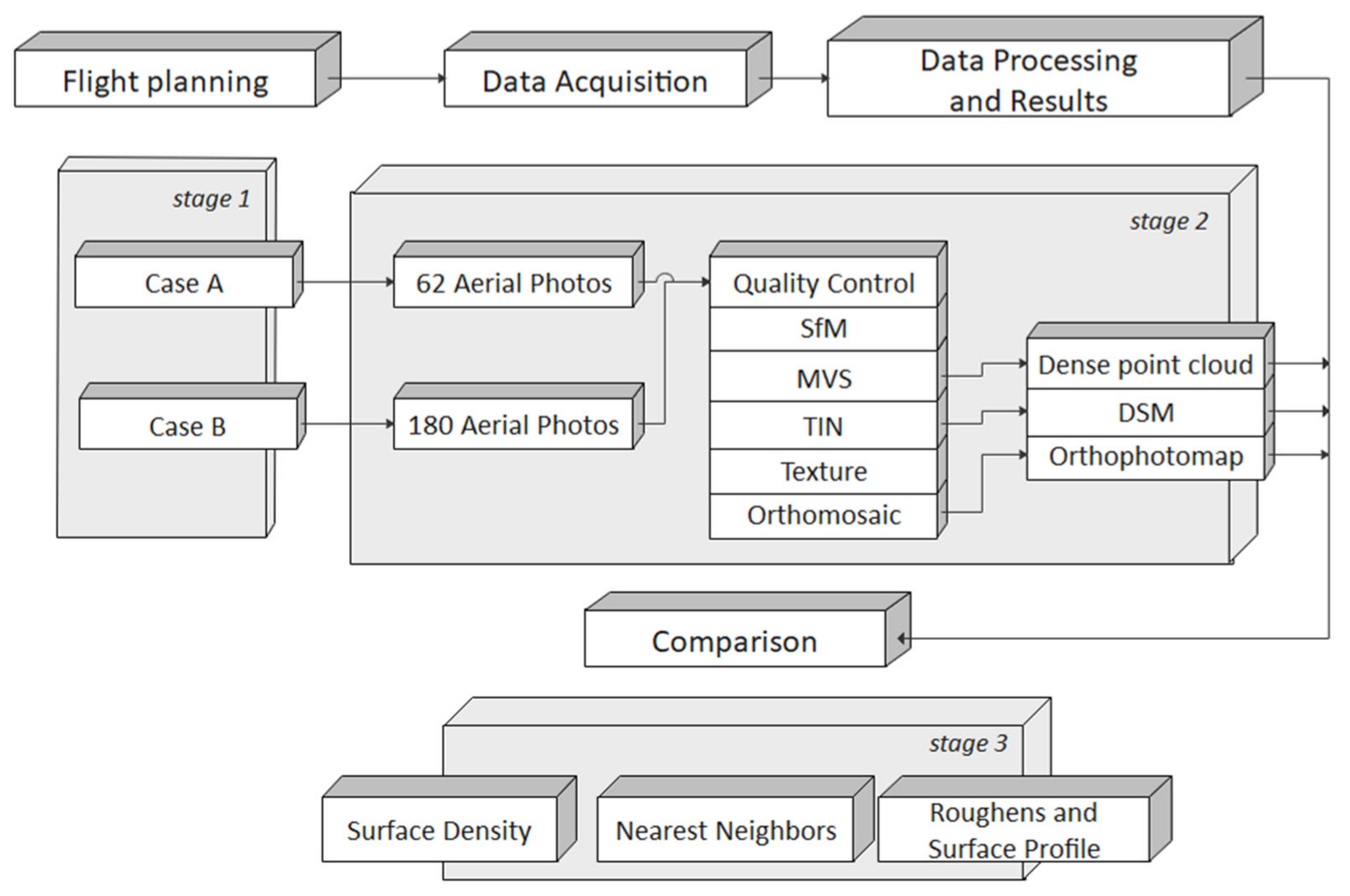
The methodology (Figure 1) consists of three main stages: (a) flight planning, (b) data acquisition and image-based 3D modelling and (c) comparison. In stage 1, two different flight plans were designed; case A and case B. Case A refers to the creation of the algorithm, as well as the preparatory work for creating a DEM-based flight plan, while case B refers to the design of a flight plan in parallel lines. In stage 2, after data collection, the images were processed using the SfM and MVS algorithms to create 2D and 3D outputs. Then follows the comparison between each of the results of the image-based 3D modelling processing, i.e., orthophotomaps, DEMs and 3D point clouds. Emphasis was given to the comparison of 3D point clouds In stage 3, surface density, number of neighbours, roughness and surface profile were the methods used to compare the point clouds [42,43].

2.1. Study Area

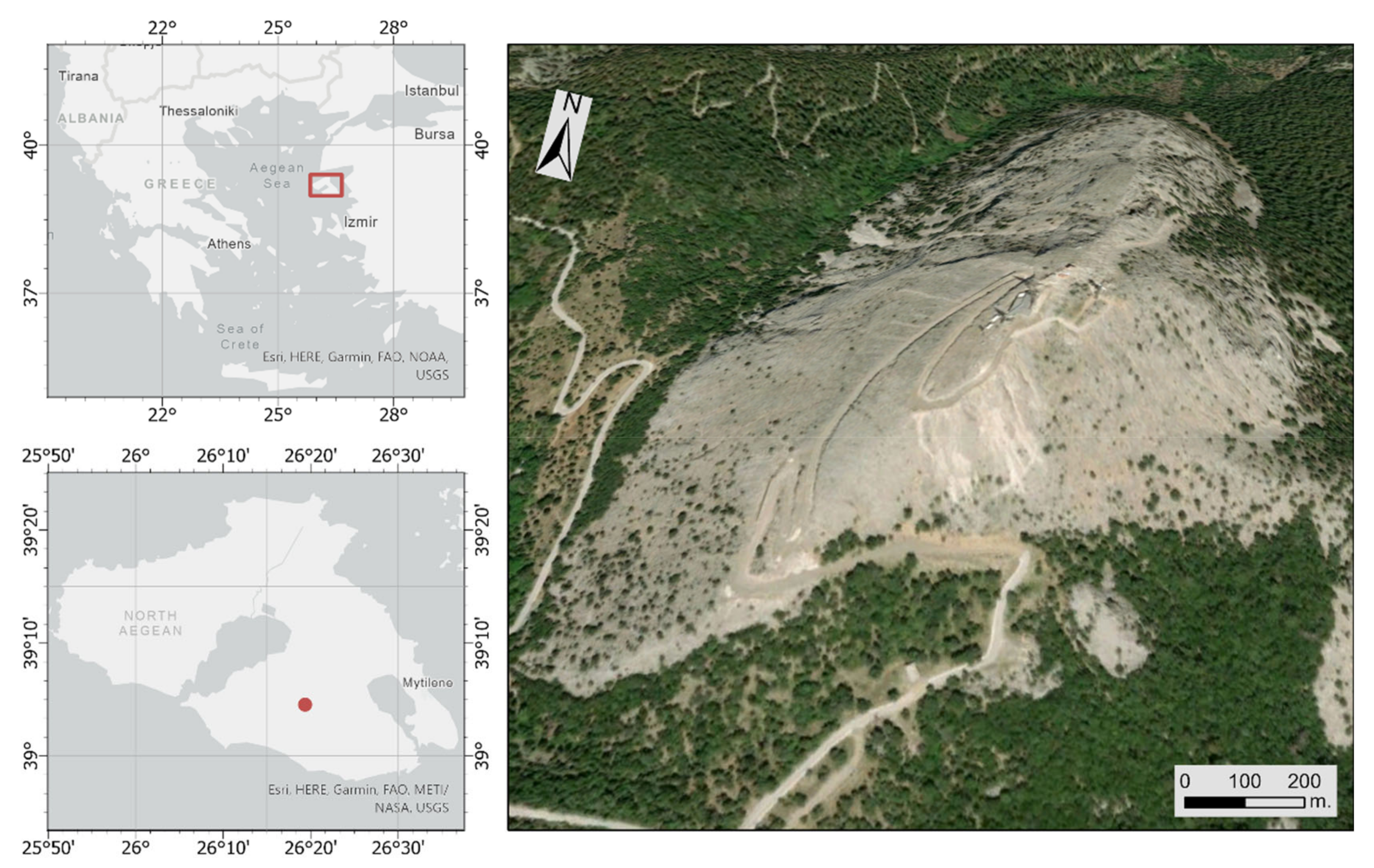
Mount Olympus, the highest peak of Lesvos island, which is situated in the northeast Aegean area, is a representative example of the complex Alpine tectonic deformation in Greece (Figure 2). In the Mount Olympus area we observe the ophiolitic nappe emplaced on top of pre-Alpine autochthonous continental terrane with a Mesozoic shallow-water carbonate platform.

After the emplacement of the allochthonous units onto the Permo-Triassic carbonate rocks of the ancient continental margin, which took place in Jurassic times, compressional events in the Late Eocene–Early Oligocene stacked several thrust sheets on the margin. This thickening of the crust in Oligocene–Early Miocene times produced the tectonic nappe formations through detachment faults and the formation of a tectonic window; Profitis Ilias peak [44,45]. Thus, Mount Olympus is considered a significant geosite of Lesvos island, revealing one of its most impressive images of a tectonic window. In the present day, the recrystallized limestone forms the impressive peak of Olympus, with the colour varying from white to ash, and sometimes even pink, with a sugary texture. Olympus mountain is a Natura 2000 site, while the area is referred to as the botanical gardens of the Aegean Sea, due to its endemic plant variety. This formation extends to an area of 17 km² and the elevation ranges between 706 m and 992 m above sea level.

2.2. Methods

The design of the flight planning begins with identifying the boundaries of the study area and determining the cartographic scale. Initially, the mapping scale of the Olympic tectonic window was set at 1:500. The flight altitude was calculated at 120 m, by taking into account the flight equipment, i.e., a DJI Phantom 4 Pro and its camera specifications (Equation (1)).

$$h=sc*fl$$

(1)

where sc describes the cartographic scale, fl is the focal length of the camera and h is the flight altitude.

The ground sampling distance (GSD) of the photographs is calculated via the flight altitude and the characteristics of the recording sensor (Equation (2)). The size of the footprints of the photos is then calculated, i.e., their image height (ih) and image width (iw) from this GSD (Equation (3)).

$$GSD=\frac{sw*h}{fl*Pw}$$

(2)

$$ih=GSD*Ph,iw=GSD * Pw$$

(3)

where GSD is ground sampling distance, sw is sensor width, sc is scale, Ph is image height (pixels) and Pw is image width (pixels).

The overlap of the images was set at 75% side overlap and 75% front overlap. Two different missions were designed for the flight planning: a) case A, which is a DEM-based flight plan and b) case B, which is a nadiral acquisition of photo sequence flight plan.

2.2.1. Case A: DEM-Based Flight Plan

The design of the DEM-based flight plan was carried out with the development of an algorithm which calculates the positions and the orientation of the camera for taking photos, by taking into account the topographic characteristics of the area as recorded in the SRTM–DEM. More specifically, the calculation of the camera position (longitude, latitude and altitude) requires the contour lines from the SRTM–DEM to be extracted with a contour interval equal to the distance of the camera position of two consecutive aerial photographs with 75% overlap and flight height 120 m (Equation (4)).

$$d_1=ih-\left(p_f*ih\right), d_2=iw-\left(p_s*iw\right)$$

(4)

where d_1,2 describes the front and side travel distance and p_f,s are the percentages (%) of the front and side overlap, respectively.

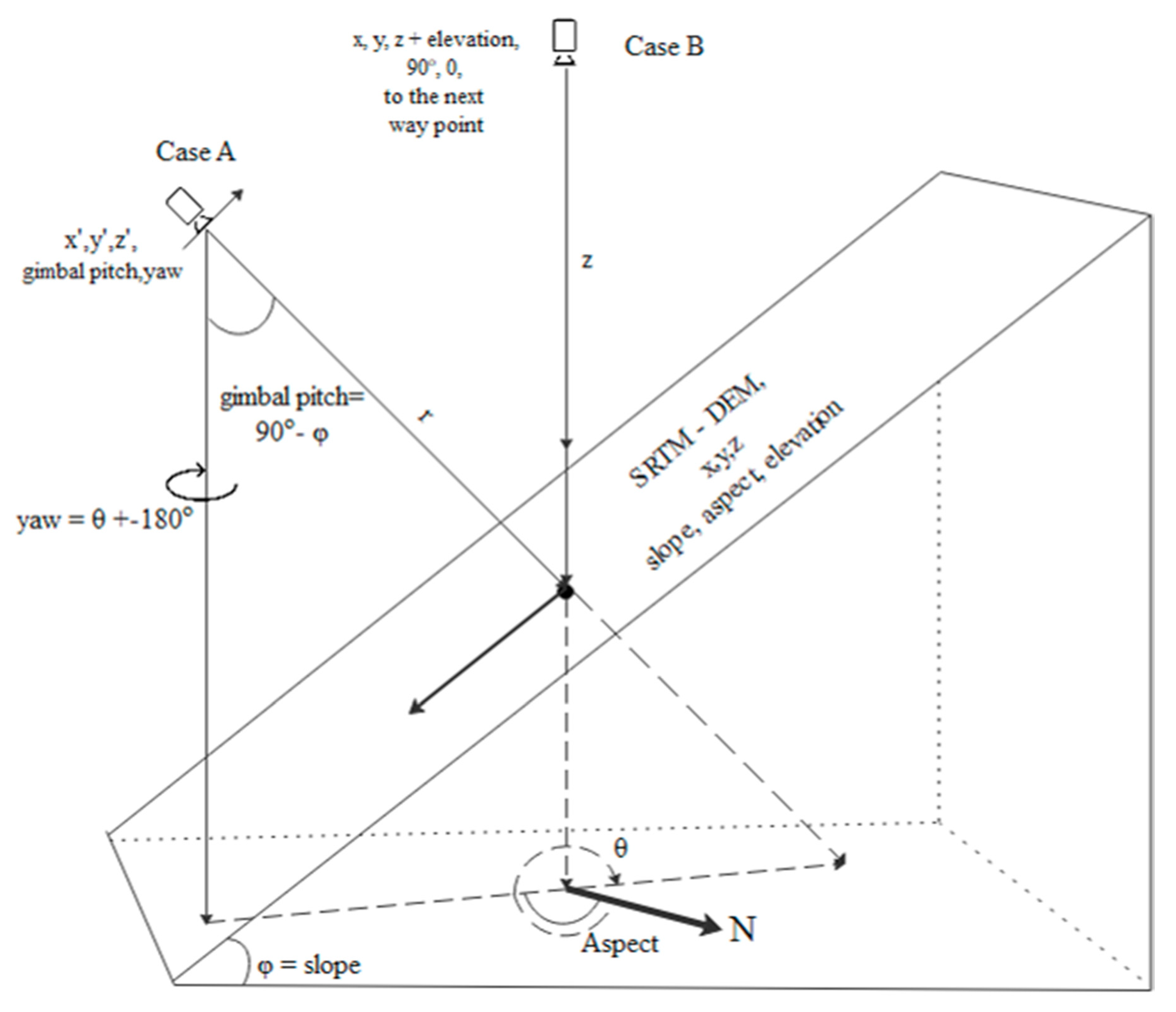
For a 75% front overlap, the contour interval is set at 30 m, while a 75% lateral overlap is achieved when the contour lines’ sections are divided into 40 m sections, equal to the distance of the camera positions of successive photographs (Equation (4)). A total of 62 points were created with coordinates of x, y and z. Taking into account the slope and aspect values of the points created by this division, the transformation described in Equation (5) is performed, resulting in the coordinates of the camera positions and the exterior orientation parameters of the photos (x′, y′, z′, roll, pitch, yaw). Moreover, the pitch of the camera was adjusted to the supplementary angle of the slope and the yaw was calculated based on the aspect, i.e., 180 degrees were subtracted from every angle larger than 180 degrees, while the reverse operation was performed in angles smaller than 180 degrees, where 180 degrees were added (Figure 3).

Hence, the camera positions, x′, y′ and z′ are calculated with:

$${\mathrm{x}}^{\prime }= \mathrm{x} + \mathrm{rsin}\mathsf{\phi }\cos \mathsf{\theta },{\mathrm{y}}^{\prime }= \mathrm{y} + \mathrm{rsin}\mathsf{\phi }\sin \mathsf{\theta },{\mathrm{z}}^{\prime }= \mathrm{z} + \mathrm{rcos}\mathsf{\phi }$$

(5)

where x, y, z are the ground point coordinates, x′, y′, z′ are the projected point coordinates (camera positions), r is the camera-object distance, ϕ is the aspect and θ is the slope. For generating the waypoints with their attributes, i.e., longitude, latitude, height of flight, yaw, pitch and roll angle, a processing model in the ArcMap model builder, ESRI (ArcMap, version 10.2.2, Software. Desktop, Esri Inc; Redlands, CA, USA, 2014), was specially designed. The input data given to that model were the SRTM–DEM and a polygon which defined the study area. The mask command was applied to the polygon that defined the area’s limits in the SRTM–DEM, and the result was used in creating the corresponding slope and aspect raster file. Then, at the contour lines generated at every 40 m, points were created at every 30 m with the split line command. The extract value command was then applied in order to extract aspect, slope and altitude values from the raster files for these points. For each point, the corresponding condition described in Equation (5) was applied to recalculate the camera positions. Each point was described by the above features in a table. The table was then exported to a CSV file, which was imported to the Mission Hub Litchi application.

The result of this process was a new point layer with redefined coordinates (62 points). These coordinates represent the photograph capture positions. The point layers were modified to the appropriate format and they were then inserted into the flight planning program. It is important to mention that this algorithm can be applied in mountainous landforms with high relief but not in flat areas.

2.2.2. Case B

The second flight was designed using Mission Hub Litchi as a nadiral photo sequence acquisition flight plan with east–west orientation, due to the study area topography. The side and front overlap were both set at 75%. The flight height remained constantly at 120 m above the ground and the angle of the camera was vertical to the ground.

2.3. Data Acquisition

Data acquisition consists of (I) performing the flights and (II) collection of photographs. A four-propeller DJI Phantom 4 Pro was used for image data collection. Its camera features include resolution: 20 Mpx, sensor width: 13.2 mm, sensor height: 8.8 mm, 24 mm focal length and 2.4 microns sensor pixel size. In addition, the Phantom 4 Pro has 3-axis stabilization (pitch, roll, yaw), a controllable range of −90° to +30° and an angular vibration range of ±0.02°. 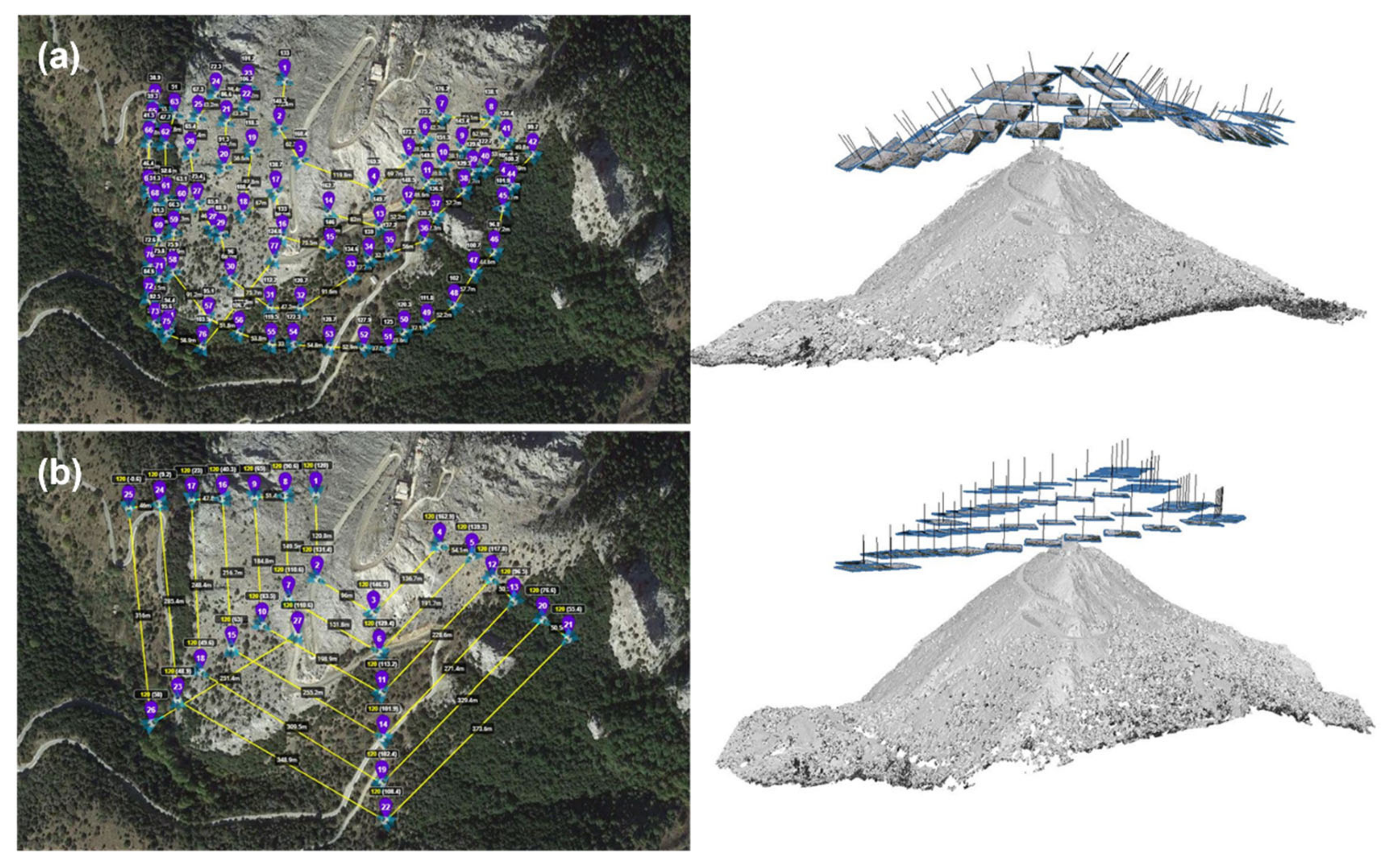The manufacturer of this UAV states that its GPS has a deviation of 0.5 m on the x, y and 2 m on the z-axis. This specific accuracy provided by the UAV’s GPS is not enough to conduct this research, and for this reason, measurements via Global Navigation Satellite Systems (GNSS) were used. Two separate flights were carried out (Figure 4a,b). The first flight, which was planned using the method described in detail above, had 62 waypoints, lasted for 16 min and the drone travelled a distance of 4 km (Figure 4a). The second flight consisted of a network of parallel lines with a distance of 40 m between them, with a constant altitude of 120 m. The orientation of the flight was from east to west, due to the topography of the study area, and 180 photos were captured (Figure 4b). The UAV travelled a distance of 5 km, with the camera angle vertical to the ground, and the flight lasted 16 min.

One of the limitations encountered during the flight plan’s execution was the flight altitude, because the UAV's GPS does not recognize the actual altitude where the UAV is, but the relative one, as it measures its take-off point as altitude 0. For this reason, one of the highest points in the study area was chosen as the take-off point. The process of performing the flights and collecting data presented some limitations such as sporadic vegetation, the nature of the terrain and the high altitude of the area. Another particularity of the present study area is the reflectivity of limestone rocks during sunny days that might result in overexposed photographs. The high flight altitude partly ensures the avoidance of obstacles, but due to altitude variations in the study area, a steady flight above the ground was chosen for the UAV in case B. This concern did not exist in case A, as for each waypoint the exact flight height had been calculated.

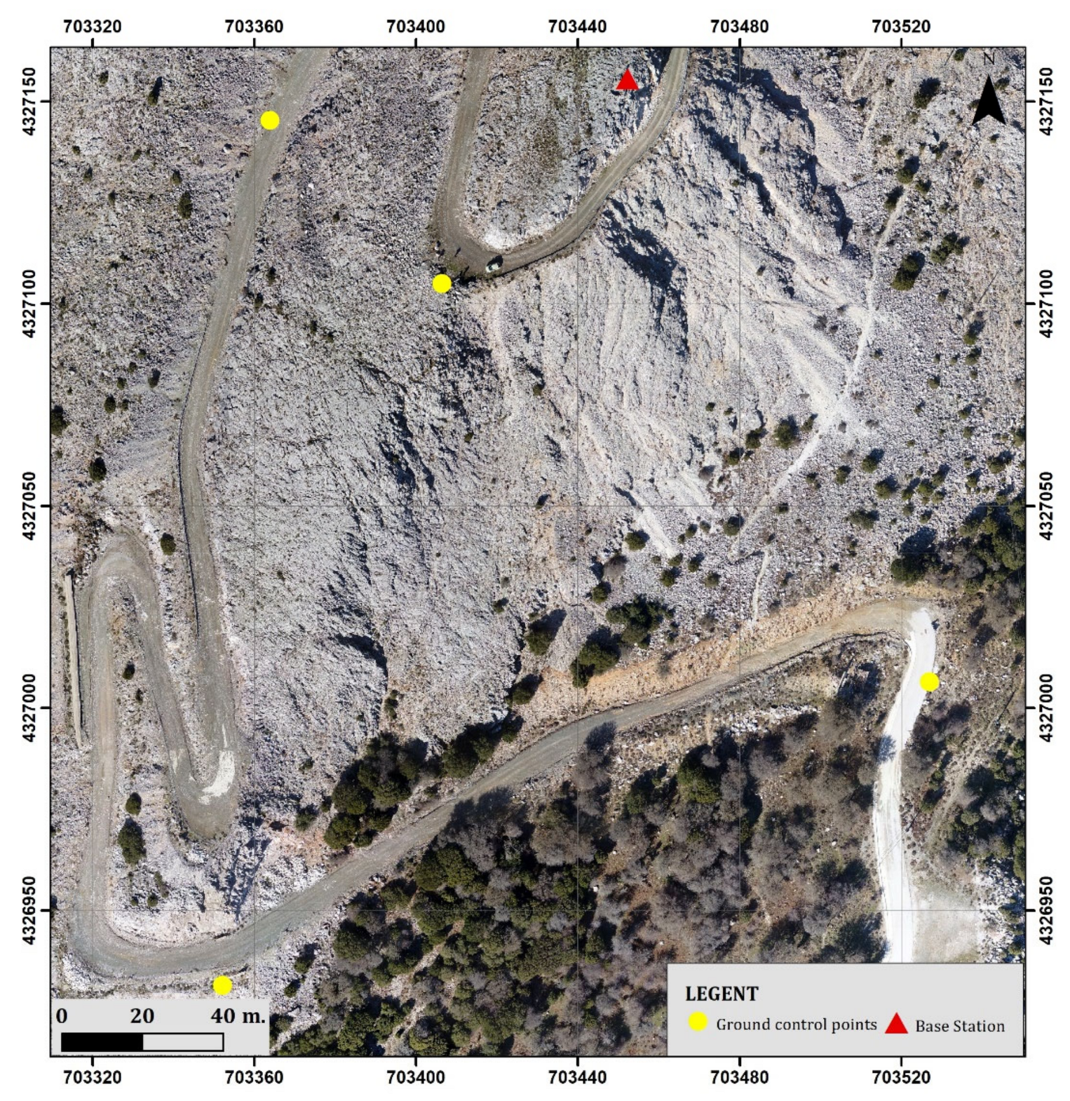
For the georeference of the collected images to be accurate, certain ground control points (GCPs) had to be measured. Those GCPs were measured using the real time kinematic (RTK) method via GNSS. More specifically, 5 ground control points (GCPs) were measured for the 2 flight plans (Figure 5), as a problem often encountered with UAVs is accurate determination of altitude [46]. The base was first placed in a trigonometric point of the Greek Army’s Geographical Service and then light-fixed points were placed around the perimeter and in the center of the study area, which were measured using a rover. One constraint encountered during the design of the GCPs network was the soil’s looseness and the intense terrain of the area, making it impossible to measure points in some areas due to the risk. The coordinate system used was the Greek Grid 1987.

2.4. Data Processing

Photogrammetric processing was performed with Agisoft, Metashape software (AgiSoft Metashape Professional Edition, St. Petersburg, Russia, Version 1.7.3) and the processing settings, i.e., alignment accuracy (medium quality) and point cloud density (high quality), in the software were the same for both data sets. Quality control of images was first executed on a visual level, and then by using the Image Quality Index (IQI) [47,48]. IQI indicates that all the images in both cases are of high quality. The camera's internal orientation is a very important factor in creating a 3D model through photogrammetric methods [49,50,51]. Previous studies have shown that when mapping flat topographies, pre-calibration of the camera model out-performs self-calibration. However, a self-calibration approach in conjunction with GNSS points might be acceptable in the case of steep topography with available convergent imagery, thus this approach is extensively applied in the literature for similar studies like in our case [52,53,54]. During the photo alignment, both internal and external camera orientation parameters, including nonlinear radial distortions, were based on the focal length extracted from EXIF metadata. The procedure is performed automatically through the Metashape software (Agisoft) and is sufficient to reach the desired accuracy on a scale of 1:500.

Τhe SfM algorithm was applied to identify a sparse point cloud. The accuracy of the alignment was medium, where images were downscaled by factor of 4 (half the resolution). The point clouds were georeferenced with 5 ground control points, RTK via GNSS, the same control points that were used in each data set. Next, the MVS algorithm was applied to create a georeferenced dense point cloud. The digital surface model (DSM) was produced from the dense point cloud. After this, photos were orthorectificated and provided the basis for the creation of a high spatial analysis orthophotomap. Data processing was done with the same settings in both data sets. Finally, the results were cropped to the same extent to be comparable, as there were differences in the point clouds borderlines.

2.5. Comparison

The next stage in this methodology is the comparison between the two flight plans created, as well as the comparison between their results after the collected images were processed. The comparison of the flight plans is first based on quality and then on quantity. The results of the data processing were a dense point cloud, a digital surface model (DSM) and an orthophotomap for each data set. The DSMs and orthophotomaps were compared on spatial resolution and sharpness level. Three different methods were used for comparing the 3D point clouds, the first one being the method of surface density. Point density is the number of points in a certain area and defines the number of measurements per area where the surface of the earth is sampled. The number of neighbours algorithm was next used as a comparison method to calculate the normal surface and the noise for each point of the neighbourhood [43]. Then the roughness and surface profiles for the two dense point clouds were calculated and compared. Roughness indicates the surface’s relief in geophysical models [42]. The measurement of the roughness value for each point is based on the distance between each point and the best fitting plane computed on its nearest neighbors; as such, it provides information about the surface’s irregularities.

3. Results and Discussion

The 3D mapping of areas with high geological importance such as geosites is crucial for their management. Appropriate data collection methodology is extremely important, as the cartographic products that emerge are tools for their study, monitoring protection and promotion. This paper presents the results of a new approach to data collection in mountainous geosites with intense geomorphology, that takes into account the slope and orientation of the area to collect very high resolution images in order to cover parts with steep and negative slopes. For the evaluation of the results, the methods applied compared the geometric characteristics of the produced 3D point clouds that emerged from case A and case B.

3.1. Photogrammetric Results

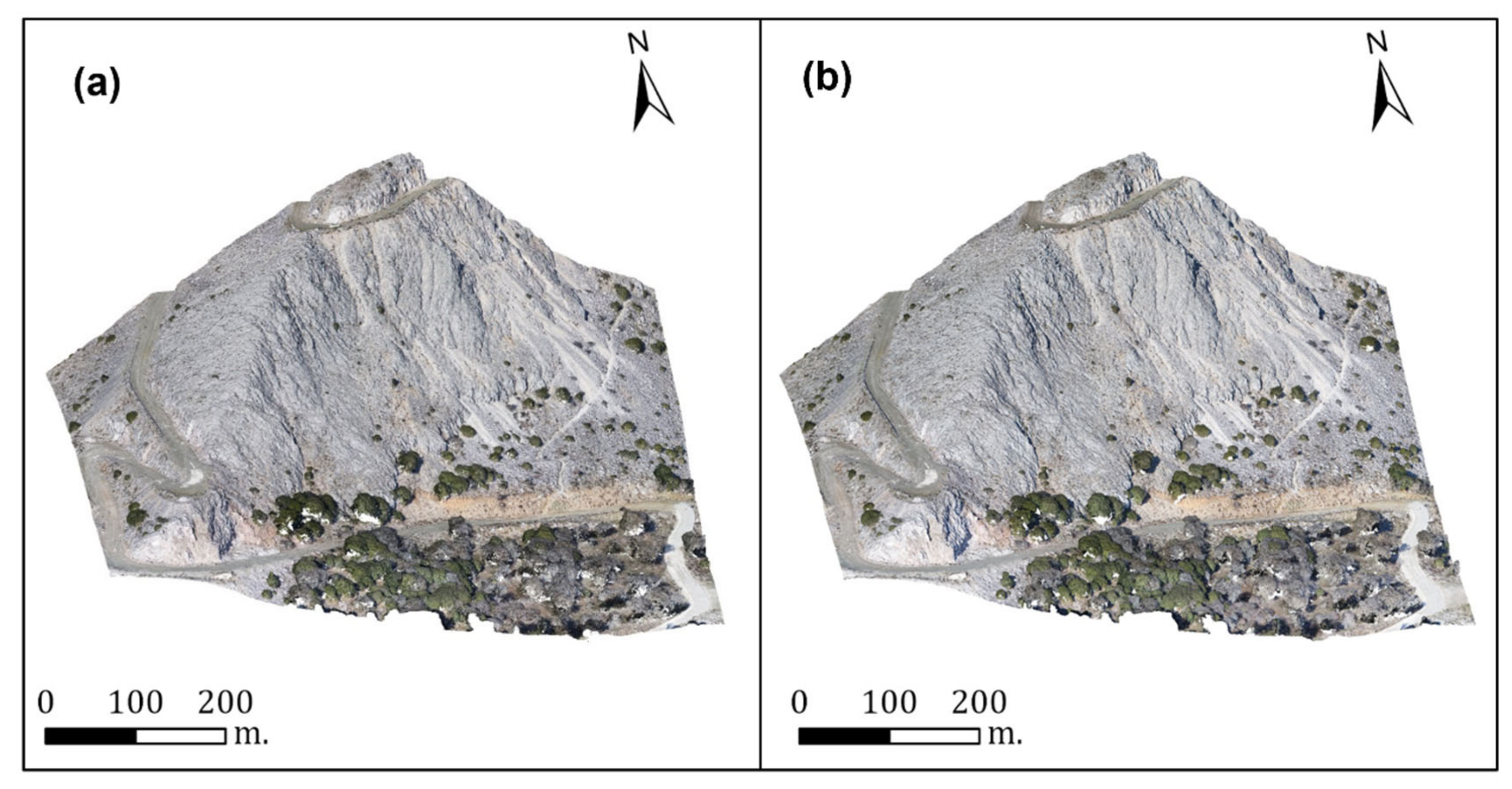
By following the conventional method, 180 images were acquired, while the proposed method resulted in 62 images. Additionally, from the set of 62 images (case A), a DSM with spatial resolution 10.6 cm and altitude values from 364–975 m (Figure 6a,b) and an orthophotomap with 5.3 cm spatial resolution (Figure 6c) were created, as well as a dense cloud point with 9,224,678 points (Figure 7a). From the set of 180 images (case B), a DSM with spatial resolution 8.66 cm and altitude values from 354 m to 975 m (Figure 6b) and an orthophotomap with 4.3 cm spatial resolution (Figure 6d) were created, and a dense cloud point with 14,503,528 points (Figure 7b). The total mapped area was 5.82 hectares in case A and 6.26 hectares in case B.

For georeferencing the data, five GCPs collected via the RTK method were used. The points used for the images georeference were the same in both cases.

Table 1. GCPs x,y,z and total RMSE in case A and case B.

Case A	X Error (cm)	Y Error (cm)	Z Error (cm)	Total (cm)
point 1	−0.0573045	−0.47308	2.93273	2.97119
point 2	−3.34445	0.14015	−1.49738	3.66704
point 3	1.45095	4.3375	12.5123	13.322
point 4	−0.638908	−3.43163	−2.27773	4.16801
point 5	2.593	−0.573001	−11.6715	11.9698
Total	2.02118	2.49647	7.85891	8.48999
Case B	X error (cm)	Y error (cm)	Z error (cm)	Total (cm)
point 1	0.630526	−0.352827	−0.232221	0.758931
point 2	−0.984104	0.198902	0.621405	1.18075
point 3	−0.808555	0.240131	−0.00987569	0.843517
point 4	−1.21827	3.94277	2.76326	4.96641
point 5	2.37962	−4.03206	−3.14346	5.63928
Total	1.354	2.5308	1.8951	3.43943

shows the errors of the total georeference and the individual points in case A and case B. More specifically, in case A, the total root mean square error (RMSE) of the georeference was 8.48 cm, and 3.43 cm in case B. In addition, Table 1 lists the errors in the accuracy of the point position for each one separately. In both cases, point 5 shows the largest deviation from its actual position, by 11.9 cm in case A and by 5.63 cm in case B.

The emerging results showed slight dissimilarities. The DSM spatial resolution in case A was lower than in case B, with a difference of 2 cm in size, while the orthοphotomaps showed a lower spatial resolution between the two outputs, with a difference of 1 cm in size. For the creation of a DSM, the Agisoft Metashape software uses the 3D point cloud. The DSM in case A had a lower resolution than in case B, because the dense point cloud of case A had a lower density of points than case B. This is because the images collected for case A were fewer than those collected for case B. The spatial resolution of the orthomosaic is calculated based on the camera characteristics and the flying altitude. The software extracts this information from the EXIFs of the images. Based on the report resulting from the georeferencing of the data and the resolution of the external orientation, the mean flight altitude was 217 m for case A and 200 m for case B. In case B, the distance along the camera view was 200 m, the same as the flying altitude, because the camera was nadiral to the terrain. In case A, the mean distance along the camera view was 193 m, which is different from the flying altitude. The difference in values is because each waypoint in case A was calculated at a different flight altitude. However, the spatial resolution of the orthomosaic is automatically defined by the Agisoft Metashape software, which does not take into account the pitch of the camera and the distance along the camera view, but instead, the flying altitude. For this reason, the spatial resolution of the orthomosaic in case A is lower than in case B. The total difference between the flight altitude from the report (case A: 217 m, and case B: 200 m) and the flight altitude (120 m) of the flight plans is due to the fact that the flight planning application (Litchi) used to collect the data, uses a DEM with low spatial resolution. As a result, it is unable to follow the extreme rough terrain of the study area with rapid changes in altitude that are observed in the specific study area within an area of DEM pixel. Hence, even if the UAV is programmed to fly at a real distance of 120 m from the terrain, after resolving the external orientation, the UAV is proved to have flown at a mean flight altitude of 217 m in case A and 200 m in case B. The above peculiarity affects the spatial resolution of the DSM and the orthomosaic because of the complexity of the area and the high altitude alteration. However, the spatial analysis of DSM and the orthomosaic in case A serves the requirements of the 1:500 scale. Moreover, dense point clouds were compared to each other on point density and distribution level.

3.2. Flight Plan and Products Comparison

The flight plans mentioned above are compared on the following levels: (a) data collection and flight characteristics, (b) data processing time and (c) results. In

Table 2. Processing characteristics of case A and case B.

	Case A	Case B
Flight duration	16 min	16 min
UAV Travel Distance	4 km	5 km
Number of photos	62	180
Dense point cloud (points)	9,224,678 pts	14,503,528 pts
DEM (spatial resolution)	10.6 cm/pix, 89.1	8.66 cm/pix, 133
	points/m2	points/m2
Orthomosaic (spatial	5.3 cm/pix	4.3 cm/pix
resolution)

, the flight characteristics are reported. The data collection time for case A was 16 min and the UAV travelled 4 km distance to cover the study area. In case B, the total duration of the flight was also 16 min and the UAV travelled 5 km in order to cover the same study area. The flight time in both cases was equal, because the UAV was programmed to stop for 2 s before taking the photo and 2 s after taking it, for each waypoint in case A. This configuration aided in reducing the number of photos that were blurry and improving image quality.

The number of photos collected was 62 in case A and 180 in case B. The produced dense clouds have 9,224,678 pts in case A, and 14,503,528 pts in case B. The DEM resolution was 10.6 cm/pix, 89.1 points/m² in case A, and 8.66 cm/pix, 133 points/m² in case B; the orthomosaic resolution were 5.3 cm/pix in case A, and 4.3 cm/pix in case B. The two flight plans’ outputs were then compared.

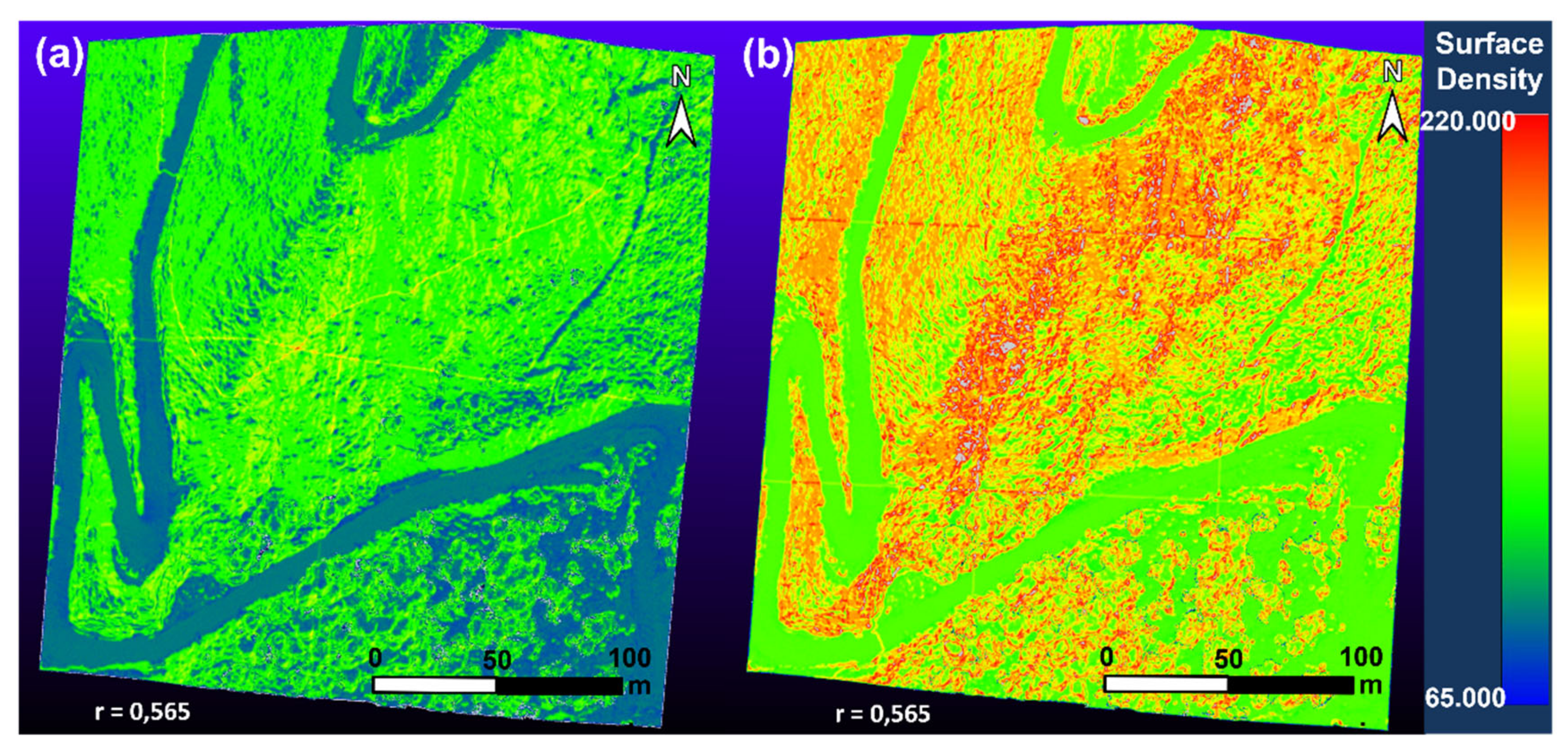
3.3. Surface Density

Figure 8 depicts the surface density of the point clouds resulting from case A and case B through CloudCompare software (CloudCompare 3D Point Cloud and Mesh Processing Software; available online: http://www.cloudcompare.org, accessed on March 2017).

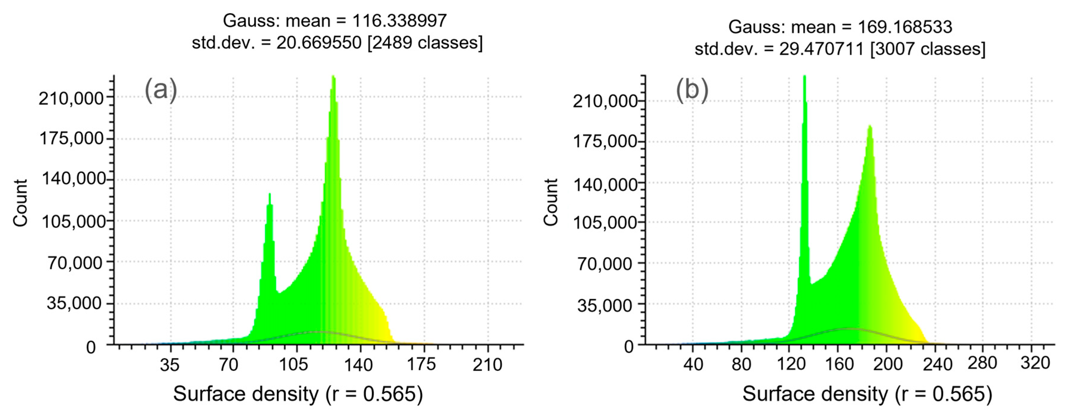
In case A (Figure 8a), there was a lower density of points along the road and a higher density on the slopes of the tectonic window. More specifically, the histogram (Figure 9a) showed a normalized distribution of points in this specific point cloud, with a higher concentration in the area of interest (more than 220,000 points with 120 pts/m² density), whereas the standard deviation was 20.66. On the other hand, the point cloud that resulted from case B showed a larger number of points but a different density in space. Figure 8b depicts a higher density of points on the high slopes of the geological structure and a lower density along the road. From the corresponding histogram (Figure 9b), it can be observed that more than 220,000 points have a density of 125 pts/m² (road) and 180,000 points have an even higher density of about 180 pts/m² (geosite), while the standard deviation is 29.47. A proportionally higher density of points along either the road or the slopes of the geosite can be noticed in case B rather than in case A. However, neither the concentration of the points nor the number of them seems to be the key factor for the rendering of the 3D reconstruction of the aforementioned man-made or natural features of a site, but the distribution of the points in space. Hence, the point cloud derived by the proposed method (case A) was lighter (9,224,678 pts), with a lower density of points (120 pts/m²—geosite, 85 pts/m²—road), compared to the one generated by the conventional method (case B), which had 14,503,528 pts with a higher density of points (180 pts/m²—geosite, 125 pts/m²—road); nonetheless, it seems that it yielded better results—mainly for the geological outcrop—due to its normalized distribution of points all around the place. A better performance of the point cloud derived from case B regarding the road, which can be explained by the flatness of the infrastructure, as the nadir photos collected depict some parts of it better and the produced point cloud has an evenly placement of its points along the road.

Based on the above observations, one can reasonably conclude that the quantity of the points does not necessarily entail a more reliable representation of a geosite in 3D; however, the way of the collection of the primary data (capture by adapting the camera’s angle on the surface’s inclination vs. “strict” vertical capture) in relation to the terrain seems to play a significant role.

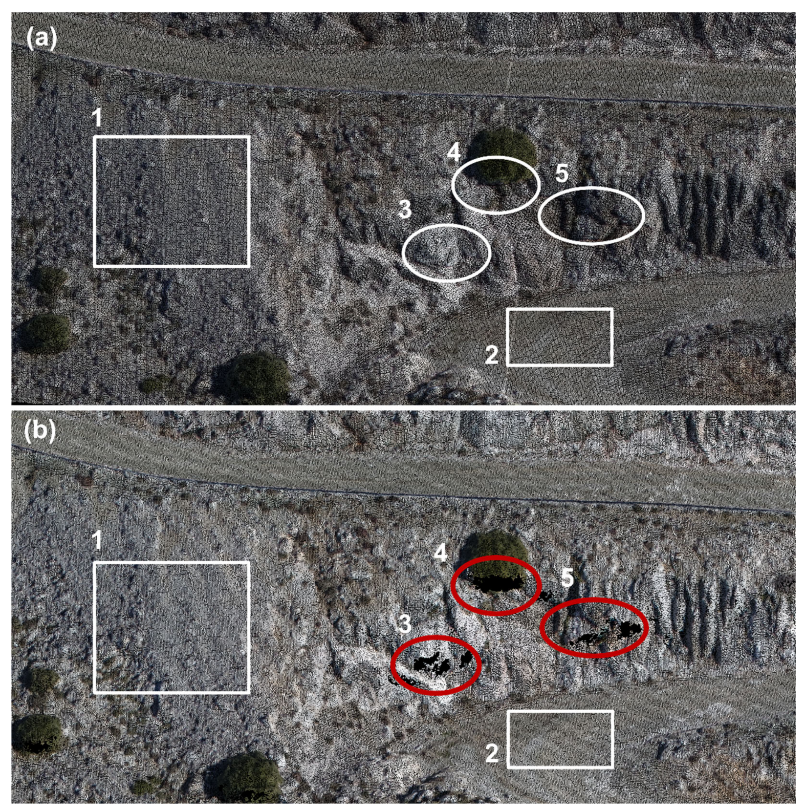
The visual quality control of the two different point clouds shows the main advantage and limitation of case A and B, respectively (Figure 10). In case B, there is an absence of points on the vertical sides of the slope which was the steepest slope in the study area (e.g., areas 3, 4 and 5 of Figure 10b), while the point cloud created in case A shows points in those specific sections. More specifically, in Figure 10a there are parts in the gentle dipping slope (Figure 10a1) with a uniform point distribution and no empty part is displayed. An identical distribution (Figure 10a2) exists in the flat sections of the road, as captured fully by the point cloud in case A. In Figure 10b, the corresponding parts of the point cloud created by the case B flight plan, i.e., pieces with gentle dipping slope (Figure 10b1) and flat parts such as the road (Figure 10b2), also show an even distribution of points and detailed display. What is particularly important and significantly differentiates case A from case B is the 3D mapping of the slope’s vertical sides or the parts with a negative gradient. In more detail, in sections 3, 4 and 5 in Figure 10a, there are points in the point cloud of the study area which have steep and negative slopes, while in case B, the corresponding parts of the point cloud for the same area have not been successfully captured and there is an absence of points, with gaps in the overall cloud. This is because flight B only collected photographs with nadiral view that do not adequately reflect the vertical surfaces of the study area. In contrast, case A, which consists of photographs with a view always orthogonal to the terrain, seems to capture the corresponding sections in more detail.

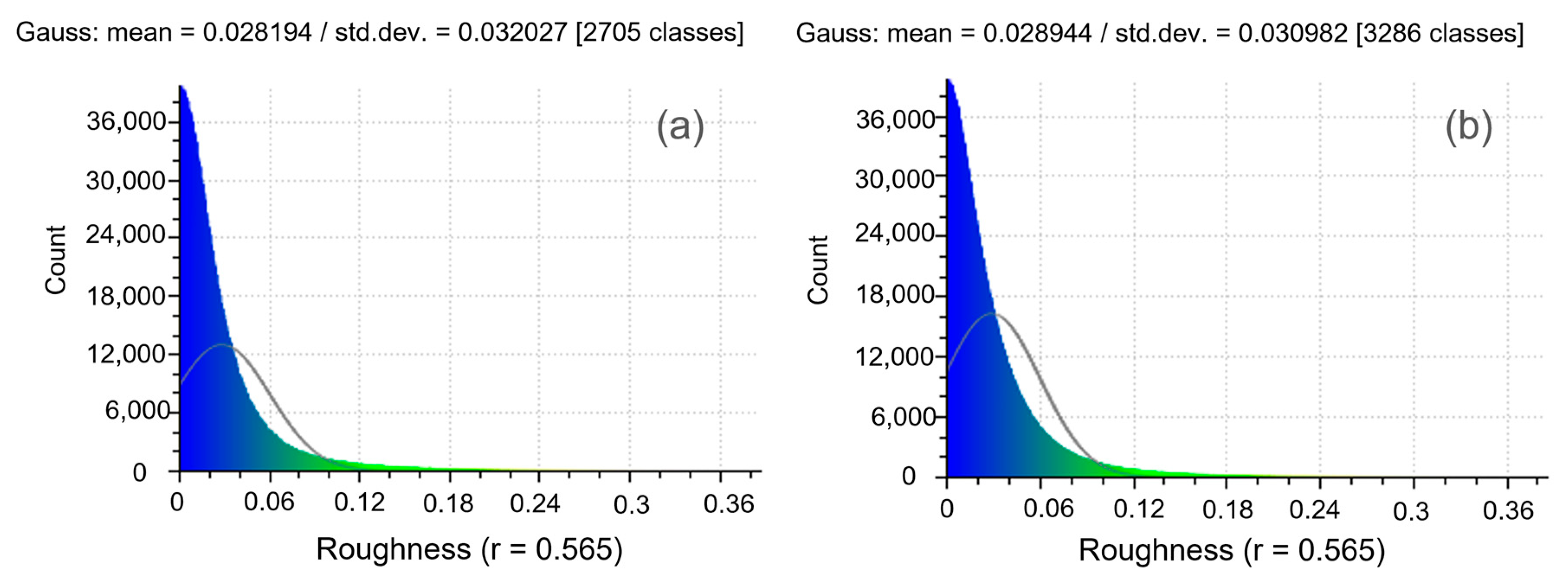
3.4. Roughness and Surface Profιle

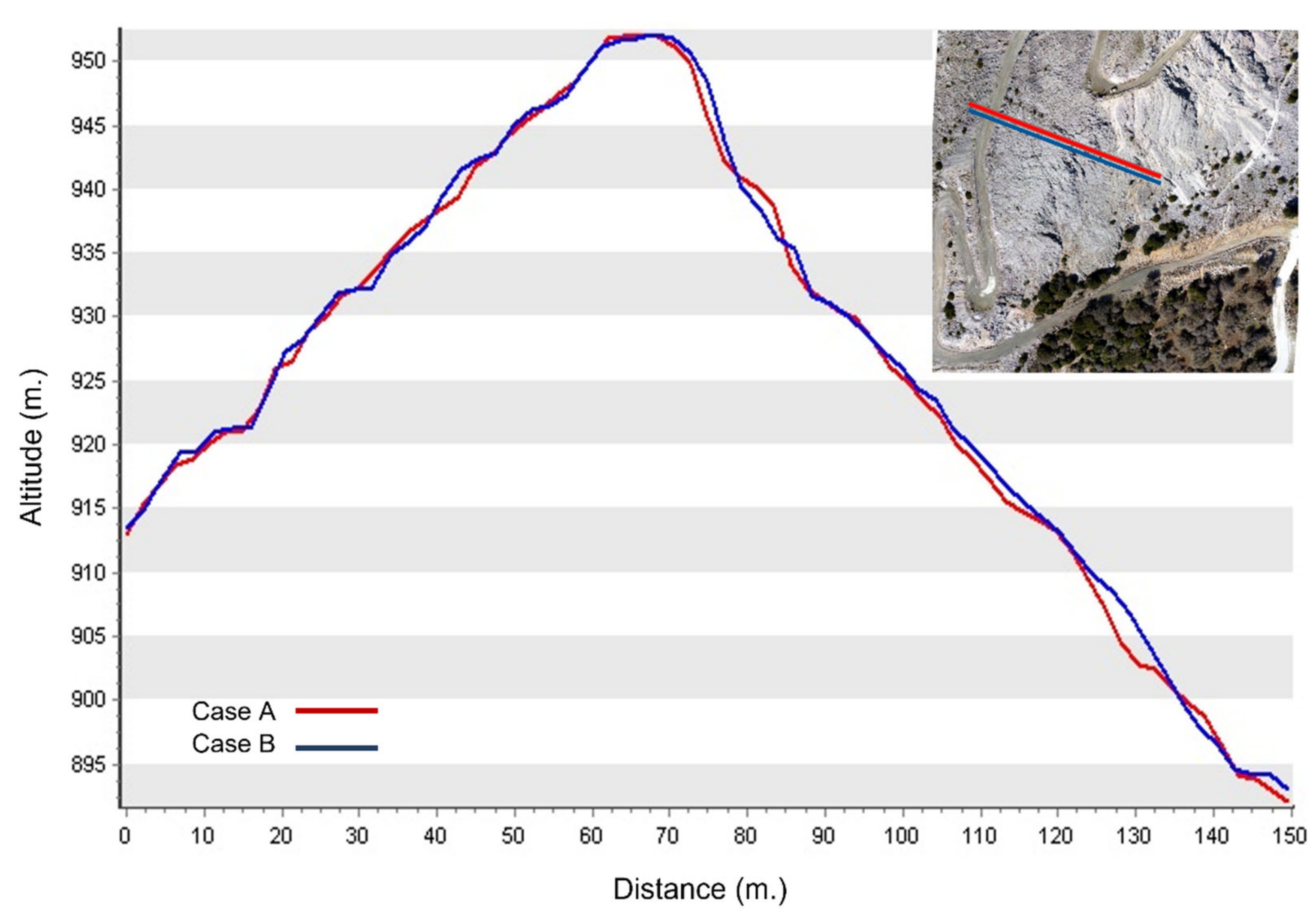
Figure 11 presents the roughness of the two point clouds. The two graphs are similar; this means that the roughness of the point clouds has almost the same curvature. In case A, the mean of the roughness per m² with a 0.565 m radius was 0.028 and the standard deviation was 0.032. In case B, the mean of the roughness with a 0.565 m radius was 0.029 per m² and the standard deviation was 0.030. Then, a section was made through the two clouds to examine the roughness and curvature on the z-axis. The section was 150 m long (Figure 12), located along the tectonic window. In this particular section, the profiles of the point clouds seem identical and have the same maximum altitude; no drastic alterations are observed in their relief. Nevertheless, these sections are not completely identical. The difference occurs due to the number of GCPs, as the northeast part of the tectonic window cannot be accessed.

4. Conclusions

Summarizing all mentioned above, this work proposes a new methodology of image collection via UAVs based on SRTM–DEM, suitable for the 3D mapping of areas with steep slopes such as in the case of mountainous geosites. This specific algorithm mentioned in the design stage of the flight for data collection for the 3D mapping of mountainous geosites is easily applied in similar cases of geomorphological structures, as it relies on open data (SRTM–DEM) which are readily available worldwide.

A digital elevation model is a significant source of information of the topography of a geosite, as it provides information about altitude, slope and aspect. In designing UAV flights, DEMs are only taken into account for the change of flight altitude, so that the scale of the photo is constant in areas with steep slopes; however, this parameter is not enough. For this reason, this paper proposes a novel methodology for creating flight plans based on the topographic features that calculates the ω, φ, κ angles of the UAV camera to capture a series of fixed scale images. The acquired photos are used to create 3D point clouds which show the presence of points on very steep slopes, in contrast to the corresponding 3D point clouds resulting from nadir photos. The comparison between the 3D point clouds shows that the 62 photos collected by the proposed algorithm for the mapping of the tectonic window of Mount Olympus produced reliable results. However, during this research, some limitations were also observed. One of these was the amount of GCPs collected from the study area. The intense and fragile terrain of the area did not allow access to various parts of the geosite, resulting in the inability to place many GCPs points. For this reason, an error of 8 cm was observed in case A, and 3.45 cm in case B. Another limitation was the weather conditions; due to the high altitude of the area, strong wind gusts affected the smooth conduct of the UAV flight.

Nevertheless, the findings of this research showed that, compared to the conventional image collection method, the results of this method are significantly advantageous, as there are no gaps in the point clouds in areas with sharp and vertical slopes, as shown by the surface density, as well as by the quality control of the clouds on a visual level. In addition, the number of photos collected from the proposed flight plan is significantly smaller (62) than the conventional method (180), which reduces the processing time. The results come in complete agreement with corresponding previous studies, which highlight the necessity of creating a flight plan for areas with irregular slopes, taking into account the values of the slope and the orientation [55].

The contribution of this study is a DEM-based flight planning that efficiently produces reliable 3D spatial information, especially in mountainous landforms where particularly high ground slope values are present. A future goal is to create a totally automated algorithm based on the DEM of the study area that effectively operates on various types of rocks and landforms. This methodology can be further exploited for 3D geomorphologic mapping and monitoring. Further investigation in the future will prove useful, by carrying out flights with LiDAR or scanning the area with a terrestrial laser scanner (TLS) and comparing the results with those of this particular methodology. In addition, the application of this methodology to other mountainous geosites around the world would be of great research interest.