A Geometric Layout Method for Synchronous Pseudolite Positioning Systems Based on a New Weighted HDOP

Abstract

The positioning accuracy of a ground-based system in an indoor environment is closely related to the geometric configuration of pseudolites. This paper presents a simple closed-form equation for computing the weighted horizontal dilution of precision (WHDOP) with four eigenvalues, which can reduce the amount of calculation. By comparing the result of WHDOP with traditional matrix inversion operation, the effectiveness of WHDOP of the proposed simple calculation method is analyzed. The proposed WHDOP has a linear relationship with the actual static positioning result error in an indoor environment proved by the Pearson analysis method. Twenty positioning points are randomly selected, and the positioning variance and WHDOP of each positioning point have been calculated. The correlation coefficient of WHDOP and the positioning variance is calculated to be 0.82. A pseudolite system layout method based on a simulated annealing algorithm is proposed by using WHDOP, instead of Geometric dilution of precision (GDOP). In this paper, the constraints of time synchronization are discussed. In wireless connection system, the distance between master station and slave station should be kept within a certain range. Specifically, for a given indoor scene, many positioning target points are randomly generated in this area by using the Monte Carlo method. The mean WHDOP value of all positioning points corresponding to the synchronous pseudolite layout is used as the objective function. The results of brute force search are compared with the method, which proves the accuracy of the new algorithm.

1. Introduction

As a commonly used positioning technology, the global navigation satellite system (GNSS) can provide service for the ground, and the ocean, in all weather conditions. However, in some more challenging situations, such as in the canyon or the indoor environment, if the number of satellites received by the receiver in these areas is less than 4, the receiver loses the ability to continue providing position information to the user [1,2,3,4]. A new positioning system is needed in these areas with weak GNSS signals, such as indoors or canyons.

In order to solve this problem, the design of pseudolites was introduced. The ground-based navigation system composed of pseudolites emits signals similar to GNSS, which can be used to enhance GNSS positioning services or even provide positioning services as an independent system [5,6,7]. In this positioning system, the position of pseudolite can be changed flexibly. However, different from GNSS, the distance between pseudolite and user is much closer than navigation satellite. Its geometric configuration has a significant influence on the whole positioning system. Like GNSS, ground-based navigation systems also use dilution of precision (DOP) to evaluate the geometric configuration [8]. As the number of satellites increases, the DOP calculation becomes larger. A lot of previous studies have been proposed to try to compute GDOP without matrix inversion or to resort to the co-factors approach [9]. These methods are mainly divided into two categories, one is based on the neural network structure, and the other is based on the extracted feature values.

Jwo and Lai used a back-propagation neural network (BPNN) for the GNSS satellite GDOP approximation [10]. Based on BPNN, these methods do not require matrix inversion operation. However, points with large deviations from the true results will appear, introducing calculation errors. In order to improve the accuracy and robustness of the network, a large amount of data is often required, which increases the computational burden. Zhu (1992) proposed a calculation method that uses the three intermediate variables a, b, and c, which significantly reduces the amount of calculation and does not require matrix inversion. However, this method is only suitable for four satellites [11]. However, in actual positioning scenarios, the receiver can often receive more than four satellites. It showed that increasing the number of satellites used for the location would reduce the GDOP and improve the positioning accuracy [12]. Thus, it makes sense to try to use all available pseudolite signals received by the receiver. Shing and Doong proposed a closed-form equation for computing GDOP for reducing the calculation based on four eigenvalues in previous studies [9]. This method can perform GDOP calculation for more than four satellites without a large amount of training data, as in the BP neural network algorithm. When people move around indoors, the height tends to be constant and people pay more attention to the horizontal orientation of the situation [4,13,14]. However, in indoor positioning scenarios, the overall positioning situation, such as different pseudolites having different variance, should be considered, instead of the size of the Horizontal dilution of precision (HDOP) value of a specific point.

To find the optimal geometric layout of pseudolites, Hu et al. [15] proposed two pseudo-satellite solutions based on airship positioning in near-space, focusing on independent airship network positioning solutions. It also points out the significant advantages of pseudo-satellites in nearby space airships. However, this method only focuses on the layout of the four pseudolites. Yi et al. [16] proposed the layout of 6 pseudolites and analyzed the influence of altitude angles and azimuth angles. However, these articles pay more attention to user positioning in the air, and most of them are based on simulation experiments without actual positioning experiments for verification and analysis. However, these methods only consider the precision factor and do not consider the differences of different pseudolites. For solving these problems in indoor ground-based systems, this paper proposes a simple calculation method for weighted HDOP concerning the eigenvalues used by Simon and El-Sherief (1995) [17] and then compared with the result of the inverse matrix operation [18] to verify the accuracy of the method. To quickly find the optimal solution of the pseudolite layout, a particle swarm optimization algorithm [19] based on simulated annealing is used. The main contributions are as follows: We analyzed the effect of the geometric distribution of the sensors on the positioning of the receivers. Then, we use a weighted calculation method to ensure a reasonable precision factor calculation. The actual system is used to verify the rationality of the proposed method. We propose a pseudolite layout algorithm, which can be used not only for pseudolite layout but also as a reference algorithm for Bluetooth and Wi-Fi layout.

In the following sections, we revisit the geometric interpretation of GNSS DOP factors and the mathematical derivation of some approximate methods in Section 2. A newly proposed method is proposed and verified through a large number of simulation experiments in Section 3. In Section 4, we conduct a real-world experiment to collect data and demonstrate the proposed algorithm with a ground-based navigation system. The Pearson correlation coefficient is calculated by using the collected static positioning results, which verifies that the proposed method has a linear relationship with the actual application. Future work and conclusions are summarized in the last section.

2. Geometric Precision Factor

In this section, we first analyze the influence of geometric accuracy factor on positioning, and then review the traditional calculation methods and existing fitting calculation methods. The fitting calculation method of WHDOP is proposed in the end of the section.

2.1. Mathematical Description of Geometric Precision Factor

The positioning principle of pseudolite is similar to GNSS, which uses the time of the satellite arriving at the user to measure the distance. A typical indoor positioning system generally consists of more than four transmission base stations. The base stations maintain time synchronization through the following methods: share a common clock source through wire connection, or maintain clock synchronization with the reference base station through wireless transmission. The receiver receives the broadcast signal of the station and then processes the signal to obtain the encoding and phase measurement values. The difference with GNSS is the multipath impact is more severe in the indoor environment. In order to reduce the impact of multipath, we usually use the carrier phase to obtain the location of the receiver. Since there is no ionosphere between the pseudolite and the receiver, the delay does not exist in the equation. Besides, because the distance between each base station and the receiver is short, the impact of the troposphere is small and can be ignored. The carrier phase observation between the ground-based station and the receiver is expressed as follows [7]:

$${\varphi }_i^k={\lambda }^{-1}∥s_i-u_k∥+N_i-f_c\delta t_i+f_c\delta t_u^k+w_i^k,$$

(1)

$$∥s_i-u_k∥=\sqrt{{(x_i-x_u)}^2+{(y_i-y_u)}^2+{(z_i-z_u)}^2},$$

(2)

where $s_i$ is the three-dimensional position of the base station i, and $u_k$ is the position of the receiver. $N_i$ stands for the ambiguity values, which are considered to be constant. In this experiment, we connect all the transmitters to the same crystal oscillator by wire. The time of all the stations can be considered well synchronized. The clock error variance of the transmitter $\delta t_i$ can be considered constant. The clock difference of receiver $\delta t_{u0}$ at the initial time and the ambiguity can be obtained in known-point-initialization (KPI) positioning method [20]. $f_c$ and $\lambda$ denote the frequency and carrier. $w_i^k$ represents other noises, such as multipath and measurement deviation, which are the main factors affecting positioning accuracy. In indoor scenes, users mostly move on a horizontal plane, the height of the receiver is constant and measurable, and the receiver only needs to solve two-position coordinate components in the horizontal direction. When we use the least square method for positioning, we only need three pseudolites to solve it. Like GNSS, the positioning accuracy of pseudolite is mainly related to the following two factors: measurement error and the geometric distribution of pseudolites. The smaller the DOP value present, the better the constellation distribution structure and the higher the positioning accuracy. The calculation of the DOP factor is based on the elements along the diagonal of matrix H [21,22], which is calculated as follows:

$$H={\left(G^{T}G\right)}^{-1}=\left|\begin{array}{cccc}{h}_{11}& & & \\ & h_{22}& & \\ & & h_{33}& \\ & & & h_{44}\end{array}\right|,$$

(3)

where

$$G=\left[\begin{array}{cccc}-cos{\theta }^{\left(1\right)}sin{\alpha }^{\left(1\right)}& -cos{\theta }^{\left(1\right)}cos{\alpha }^{\left(1\right)}& -sin{\theta }^{\left(1\right)}& 1\\ -cos{\theta }^{\left(2\right)}sin{\alpha }^{\left(2\right)}& -cos{\theta }^{\left(2\right)}cos{\alpha }^{\left(2\right)}& -sin{\theta }^{\left(2\right)}& 1\\ \cdots & \cdots & \dots & \dots \\ -cos{\theta }^{\left(N\right)}sin{\alpha }^{\left(N\right)}& -cos{\theta }^{\left(N\right)}cos{\alpha }^{\left(N\right)}& -sin{\theta }^{\left(N\right)}& 1\end{array}\right].$$

(4)

The matrix H ultimately depends on the number of visible satellites and the geometric distribution relative to the positioning users and has no relationship with the signal strength of pseudolites or the quality of receivers. The corresponding DOP values can be calculated according to the weight coefficient matrix H. Usually, we use GDOP to observe geometric accuracy, HDOP to indicate horizontal accuracy, and Vertical dilution of precision (VDOP) to observe vertical height precision. They are calculated as follows:

$$\mathrm{GDOP}=\sqrt{h_{11}+h_{22}+h_{33}+h_{44}},$$

(5)

$$\mathrm{HDOP}=\sqrt{h_{11}+h_{22}},$$

(6)

$$\mathrm{VDOP}=\sqrt{h_{33}}.$$

(7)

Note that the DOP definition assumes that all tracking pseudolites of the system measurements have the same accuracy. However, these measurements of different pseudolites have different variances, especially when the elevation difference is enormous. When the pseudolite is installed at a high altitude from the ground, the elevation is low when the receiver is far away from the pseudolites. The multipath effect is more severe than that of the satellite with high elevation. Therefore, the proper weighting measurement of a single satellite should be considered. The weighted GDOP (WGDOP) [23] has been put forward as follows:

$$\mathrm{WGDOP}=\sqrt{tr\left[{\left(G_N^T{W}_N{G}_N\right)}^{-1}\right]}.$$

(8)

The weighted matrix is expressed as:

$$W_N=diag(\frac{1}{{\sigma }_1^2}\dots \frac{1}{{\sigma }_N^2}).$$

(9)

The method for calculating the variance of the measures adopted in Pan et al. [24] is given by:

$${\sigma }_i^2={\sigma }_0^2/{\left(sinE\right)}^2.$$

(10)

${\sigma }_0$ is the standard deviation (STD) of code observations, which is different for each constellation. E is the satellite elevation angle and stands for the satellite elevation angle, and ${\sigma }_0$ is different for different GNSS constellations. Since there is only one constellation in ground-based navigation, we set the value to 1. Similar to the calculation method of WGDOP, our proposed WHDOP uses the same weight matrix as follows:

$$W_N=diag(sin{E}_1^2\dots sin{E}_i^2...sin{E}_N^2).$$

(11)

2.2. Fitting Algorithm of GDOP

In order to reduce the amount of calculation, Simon used the artificial Neural Network (ANN) approach for GDOP approximation. There are two stages of operation in the neural network method. First, data with known associated pairs is sent to the network for learning weights in the training phase. The goal is to minimize the difference between the output of the network and the real output. Researchers spent four hours and 47 min on VAX machines to train satisfactory artificial neural networks. The final root mean squared error (RMSE) was 1.44%.

From their point of view, the calculation of DOP consists of four independent eigenvalues, and the GDOP can be expressed as:

$$\mathrm{GDOP}=trace\left(H\right)=\sqrt{{\lambda }_1^{-1}+{\lambda }_2^{-1}+{\lambda }_3^{-1}+{\lambda }_4^{-1}}.$$

(12)

The selection of eigenvalues is defined as follows:

$$h_1\left(\lambda \right)\equiv {\lambda }_1+{\lambda }_2+{\lambda }_3+{\lambda }_4=trace\left(H\right),$$

(13)

$$h_2\left(\lambda \right)\equiv {\lambda }_1^2+{\lambda }_2^2+{\lambda }_3^2+{\lambda }_4^2=trace\left(H^2\right),$$

(14)

$$h_3\left(\lambda \right)\equiv {\lambda }_1^3+{\lambda }_2^3+{\lambda }_3^3+{\lambda }_4^3=trace\left(H^3\right),$$

(15)

$$h_4\left(\lambda \right)\equiv {\lambda }_1{\lambda }_2{\lambda }_3{\lambda }_4=det\left(H\right).$$

(16)

Shing and Doong presented a simple closed-form equation for solving this equation by using Newton’s identities from symmetric polynomials [9]. Cubic elementary symmetric quaternion polynomial can be written down as:

$$e_3(X_1,X_2,X_3,X_4)=X_1{X}_2{X}_3+X_1{X}_2{X}_4+X_1{X}_3{X}_4+X_2{X}_3{X}_4.$$

(17)

It can be written as follows by using Newton’s identities:

$$e_3=\frac{1}{3}[\frac{1}{2}(p_1^2-p_2)p_1-p_1{p}_2+p_3],$$

(18)

where p stands for the power sum symmetric polynomial of degree k, for example:

$$p_k(X_1,X_2,\dots ,X_n)=X_1^k+X_2^k+\dots +X_n^k.$$

(19)

The expression of GDOP can be expressed as:

$$\mathrm{GDOP}=\sqrt{\frac{{\lambda }_1{\lambda }_2{\lambda }_3+{\lambda }_1{\lambda }_2{\lambda }_4+{\lambda }_1{\lambda }_3{\lambda }_4+{\lambda }_2{\lambda }_3{\lambda }_4}{{\lambda }_1{\lambda }_2{\lambda }_3{\lambda }_4}}.$$

(20)

After the above theoretical calculations, the final approximate expression is as follows:

$$\mathrm{GDOP}=\sqrt{\frac{0.5h_1^3-1.5h_1{h}_2+h_3}{3h_4}}.$$

(21)

2.3. WHDOP Fitting Algorithm

The GDOP value obtained by the calculation method in Equation (21) does not need to be inverted. Which reduces the amount of calculation and does not incur any approximation error nor require much training. Since these four eigenvalues are derived from elevation and azimuth, they can also be used to calculate HDOP. This paper proposes a weighted HDOP calculation method with the same form as GDOP, as follows:

$$\mathrm{WHDOP}=\sqrt{\frac{a{h}_1^3+b{h}_1{h}_2+c{h}_3}{d{h}_4}}.$$

(22)

Among them, abcd is a fixed coefficient. When the scene is fixed, abcd has a set of optimal solutions to minimize the residuals between weighted HDOP solved by traditional algorithms and the proposed method. We use a genetic algorithm to find the suitable value of abcd. A genetic algorithm is a kind of random optimization derived from the evolution of the survival of the fittest. Unlike traditional search algorithms, we can process multiple individuals in the group simultaneously by using genetic algorithms. This means that multiple search space solutions are evaluated, reducing the risk of falling into a locally optimal solution. The genetic algorithm does not have the limitation of function continuity in the derivation. Directly operating on structural objects is one of the main features of the algorithm. Genetic algorithm uses a probabilistic method to find the optimal solution, which has a certain inherent, implicit parallelism and good global optimization capabilities. When the information is obtained in the evolution process to organize the searching, individuals with more excellent fitness have a higher survival probability. They are more adapted to the environmental and genetic structure. The search direction can be adjusted adaptively, and the optimized search space can be automatically obtained and guided when searching for the optimal value. In summary, the genetic algorithm is suitable for solving the four-parameter problems.

The specific steps are as follows: first, randomly generate 4N initial data for abcd, which constitutes a group. We use these 4N random data as a starting point and iteratively update. In the biological world, the fitness of the theory of evolution represents the ability of an individual to adapt to the environment. Here, we use this fitness function as an evaluation indicator and the objective function to be optimized. In the genetic algorithm, the fitness function needs to be compared and sorted. The selection probability is calculated on this basis at the same time, so the value of the fitness function should be positive. We randomly select dozens of points in the indoor positioning scene and use traditional methods as function 6 and function 8 to calculate their WHDOP values. Then, the sum of the absolute value of the difference with the proposed method is also called as L1-norm is used as the fitness function, as follows:

$$F{}_{fitness}=\sum _{i=1}^{N}abs(\mathrm{WHDOP}{i}_{proposed}-\mathrm{WHDOP}{i}_{troditional}).$$

(23)

Afterward, through selection, excellent individuals are selected from the exchanged groups so that they have the opportunity to reproduce as parents for the next generation. The process to find the smallest value of the fitness function. The next step is mutation. A certain number of individuals are randomly selected in the group. The value of a gene in the data is randomly changed with a certain probability for the selected individuals, just as in biological evolution. In genetic algorithms, the probability of mutation is low, and this value is usually between 0.001 and 0.01, which provides an opportunity for new values to be generated. Finally, we should stop the program when the required deviation is satisfied, or the algorithm iteration reaches the maximum genetic algebra. When we get the calculation method of WHDOP, we can use it to carry out the geometric layout of the base stations.

Pseudolites are often placed on the top of the house to make more places have direct signals and avoid obstacles in the indoor environment. All the WHDOP values of indoor positioning points will also change accordingly when the position of one of the pseudolites is changed. Therefore, selecting a suitable location for all the pseudolites requires many calculations to have a reasonable WHDOP for all potential points to be located. In order to obtain this solution quickly, we adopted an improved particle swarm algorithm based on the simulated annealing algorithm.

The simulated annealing algorithm is inspired by the simulation of the reliable cooling process. When the solid is heated, the thermal motion of the atoms in the solid increases continuously, and the internal energy increases. As the temperature rises, the orderly movement of the solid particles is broken. The particles inside the solid become disordered with the increase in temperature. The particles gradually tend to be ordered as the temperature of the object decreases and, finally, reaching the ground state at room temperature, where the internal energy is also the smallest. It is a theoretically global optimal algorithm, which has been widely used in engineering.

We set the internal energy as the objective function value and consider the temperature T as a control parameter in actual application. The simulated annealing algorithm has no relation to the initial value, and the solution obtained by the algorithm has no relation to the initial solution. Simulated annealing is an algorithm with asymptotic convergence.

Starting from a random solution, a new candidate value is randomly generated from the domain. The acceptance criterion allows the objective function to accept the solution that deteriorates the objective function within a specific range. The optimization process is to continuously generate new solutions (different pseudolite geometric distributions), calculate the objective function, and choose to accept or reject this result according to a certain probability. In the particle swarm algorithm, if the best position of the group is at the local minimum, all particles tend to the local minimum. We can improve the particle swarm algorithm and increase its global search ability by using simulated annealing.

The original particle swarm algorithm updates the speed and position of the particles as follows, where $x_{i,j}$ is the position of the pseudolite, $cr$ represents the random probability, $c_1$ and $c_2$ are set to 2.1, and $p_g$ represents the local best value. The number of populations of the particle swarm algorithm is set to 40, the maximum number of iterations is 100, and the total number of calculations is 4000.

$$v_{i,j}(k+1)=\chi [v_{i,j}\left(k\right)+c_1{r}_1(p_{i,j}\left(k\right)-x_{i,j}\left(k\right))+c_2{r}_2(p_{g,j}\left(k\right)-x_{i,j}\left(k\right))],$$

(24)

$$\chi =\frac{2}{\left|2-(c_1+c_2)-\sqrt{{(c_1+c_2)}^2-4(c_1+c_2)}\right|}$$

(25)

$$x_{i,j}(k+1)=x_{i,j}\left(k\right)+v_{i,j}(k+1)(j=1,\dots ,n).$$

(26)

In order to minimize the overall WHDOP value, the objective function is set as follows:

$$F=\mathrm{WHDO}{P}_1+\mathrm{WHDO}{P}_2+\mathrm{WHDO}{P}_k+\dots +\mathrm{WHDO}{P}_n,$$

(27)

where $\mathrm{WHDO}{P}_k$ represents the value of weighted HDOP of the k-th positioning point relative to the current pseudolite geometric distribution. In order to meet the requirements of time synchronization, the distance between the slave station and the master station should be kept within a certain range.

$$∥s_0-s_i∥\le d_{max}.$$

(28)

$s_0$ indicates the location of master station, $s_i$ indicates the slave station. $d_{max}$ is the maximum distance of wireless communication. The first step is to generate a new variable in the solution space. In order to reduce the time complexity of the algorithm, a method that can generate a new solution through simple transformation is usually selected, such as replacing or swapping all or part of the candidate values. We select a $p_i$ position to replace $p_g$ with a certain probability of avoiding the algorithm falling into the local minimum solution. The second step is to calculate the objective function difference corresponding to the new candidate value. The calculation equation is as follows:

$$\Delta F=F_{p_i}-F_{p_g}.$$

(29)

The third step is to judge whether the new solution is accepted. The calculation method of probability is as follows: min{1, exp($-\Delta F$ /T)}> random [0, 1]. If this calculation is satisfactory, we choose to accept the new solution. The last step is to modify the objective function value when the new candidate value is determined to be accepted. The current solution has completed one iteration when this step is done. The next round of iteration is carried out based on the current solution. However, if the new candidate value is judged to be discarded, the next round of trials will continue based on the original solution. After many solution changes, we can find the minimum value of the objective function under a specific T and, finally, obtain the optimal global pseudolites distribution solution.

3. Simulation Experiment of the Proposed Algorithm

In this section, we first introduce the method of fitting WHDOP, and then propose the layout method. We analyze the time complexity of the proposed method. In the last part of this section, we conduct test experiments in a real environment.

3.1. Simulation for Calculating WHDOP

We conducted simulation experiments to verify the accuracy of the proposed algorithm for WHDOP calculation. Assume that the positioning area is a 7 × 9 m rectangle, and the pseudolites are installed at the height of 8 meters in this positioning area. To solve the four unknown solutions of abcd in Equation (22), we randomly generated 100 points in the positioning area and randomly generated six pseudolite coordinates, as shown in Figure 1. We calculated the WHDOP value of each point by using the traditional method. Then, we put these WHDOP into Equation (23) and use the genetic algorithm to solve the unknown parameter abcd.

The values of abcd obtained are: −0.259, 0.173, 0.132, 1064.355. To verify the accuracy of the proposed WHDOP algorithm, we use the Monte Carlo method [25] to randomly generate 500 points in the area and calculate the value of WHDOP by two methods for each point. We randomly changed the coordinate position of the pseudolites and performed it ten times in total. The average error of all points WHDOP is 0.743. The mean value of WHDOP is 12 under the traditional method. We drew the difference between the two values of 50 points, as shown in Figure 2.

An example for computing WHDOP is illustrated. Suppose a random distribution of 6 pseudolites is available to the receiver, and the direction cosines as follows:

$$G=\left|\begin{array}{cccc}-0.343& 0.316& -0.885& 1.0\\ -0.120& 0.125& -0.985& 1.0\\ -0.351& 0.440& -0.826& 1.0\\ -0.410& 0.159& -0.898& 1.0\\ -0.593& 0.169& -0.788& 1.0\\ -0.630& -0.148& -0.763& 1.0\end{array}\right|,$$

(30)

$$W=[0.783,0.970,0.683,0.807,0.0620,0.582],$$

(31)

$$H=G^{{}^{\prime }}diag\left(W\right)G,$$

(32)

$$H=\left|\begin{array}{cccc}83.834& -18.518& 170.532& 183.701\\ -18.518& 12.141& -35.098& -39.817\\ 170.532& -35.098& 386.412& 407.613\\ 183.701& -39.817& 407.613& 432.163\end{array}\right|.$$

(33)

Then, get the value of h₁ through trace(H), and get the value of h₂ and h₃ through trace(H²) and trace(H³). The values of h₁, h₂, h₃, and h₄ are 8.889, 74.100, 637.300, $1.701\times {10}^{-4}$. According to the traditional calculation method, we can get the value of WHDOP is 9.797. The WHDOP result obtained by using Equation (22) is 9.449. According to the method of six pseudolites, we also carried out the calculation of four pseudolites and eight pseudolites and summarized the results in

Table 1. Fitting parameters and errors under different numbers of pseudolites.

Number of Pseudolites	4	6	8
a	−0.295	−0.259	−0.656
b	0.401	0.173	0.394
c	−0.052	0.132	0.387
d	313	1064	1995
Mean WHDOP value	14.072	12.002	6.843
Average error	1.134	0.743	0.643
Error percentage	8.66%	6.19%	9.40%

. It should be noted that, when randomly generating the pseudolite distribution, we avoided the case where the pseudolite distribution is concentrated or linear and chose the relatively scattered geometric distribution of pseudolites for calculation. This is also in line with the situation when the ground-based system is deployed, making the overall DOP in the positioning area small.

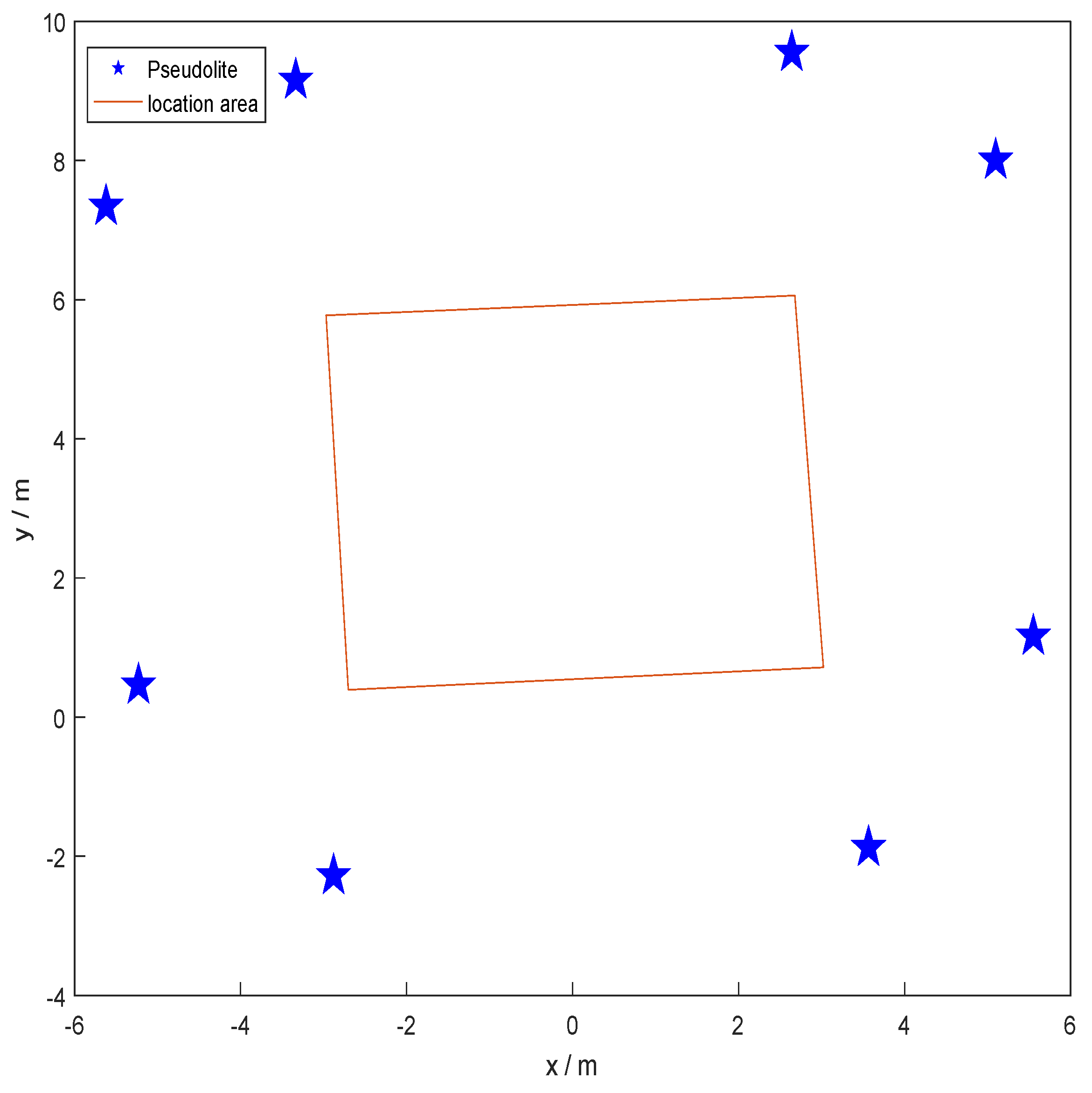
3.2. Pseudolites Geometric Planning Simulation

Assume that the positioning area is a 7 × 9 m rectangle, and the pseudolites are installed at the height of 8 m in this positioning area, which is the same as 3.1. We used the improved particle swarm algorithm based on simulated annealing to simulate the geometric layout of pseudolites. We set the number of iterations N to 100. The actual iteration process can be seen from Figure 3, where the algorithm has converged when N = 32.

From the operation results, the improved geometric layout method of pseudolites has good convergence and robustness. In terms of time complexity, it is $O(N^{{}^2})$ and does not change with the number of pseudolites. In computer science, brute force or exhaustive search [26], also known as generating and test, can provide global optimal solutions. The method consists of systematically enumerating all possible candidates for a solution and checking that each candidate matches the problem description. Although brute force research is easy to implement, if a solution exists, it will certainly find it. However, its cost is proportional to the number of candidate solutions, and, due to this, in many practical problems, the cost consumed grows rapidly with the size of the problem. The results of the brute force search algorithm are more accurate but consume a lot of computing resources. We can use the results of the brute force search algorithm to verify the accuracy of our proposed algorithm. If we use the brute force search method, as the number of pseudolites increases, the computational time complexity will increase exponentially. We use four pseudolites to conduct a brute force search and compare the results with the proposed method. The search process is as follows, assuming that, with 1 meter as the step unit, the x-coordinate range of pseudolite one starts from 0 to 9, and the y-coordinate range is 0 to 7. The other three pseudolites are traversed at the same time as the first pseudolite. In the process of searching, the average WHDOP value at each group of positions is recorded. After traversing all positions, the position distribution of the pseudolites with the minimum WHDOP solution is found. The time complexity of the algorithm is $O\left(N^4\right)$ in terms of time complexity. This process requires ${(9\ast 7)}^4=$ 15,752,961 operations. The time complexity increases exponentially with the number of pseudolites. We need to multiply the calculation of WHDOP by 500 points to get the total calculation amount. Due to the limited computing resources, we could only perform a global brute force search of 4 pseudolites. In order to verify the accuracy of the proposed method, we plot the results of two different methods, as shown in Figure 4.

We put the distribution results of WHDOP in

Table 2. Distribution of WHDOP values using different methods under four pseudolites.

WHDOP Value	≤4	4–5	5–6	>6	Mean WHDOP
Proposed Method	41.8%	21.6%	13.8%	22.8%	4.8
Brute Force Search	39.4%	26.6%	14.0%	20.0%	4.7

. The average WHDOP value of the proposed method and brute force search is only 0.1, (2%), indicating the accuracy of the proposed method.

We simulated the layout of six pseudolites and eight pseudolites, as shown in Figure 5 and Figure 6. There is a pseudolite at every corner and center, which makes the overall WHDOP value small. Then, we make statistics of WHDOP results, as shown in

Table 3. Distribution of WHDOP values using the proposed method under six pseudolites and eight pseudolites.

WHDOP Value	≤4	4–5	5–6	> 6	Mean WHDOP
6 pseudolites	78.0%	10.2%	10.8%	1.0%	2.958
8 pseudolites	85.8%	8.2%	5.8%	0.4%	2.694

.

In this positioning area, from four pseudolites to six pseudolites, WHDOP decreased by 1.888. However, the WHDOP decreased by 0.264 from six pseudolites to eight pseudolites, indicating that the distribution of six pseudolites has a good positioning accuracy in this area.

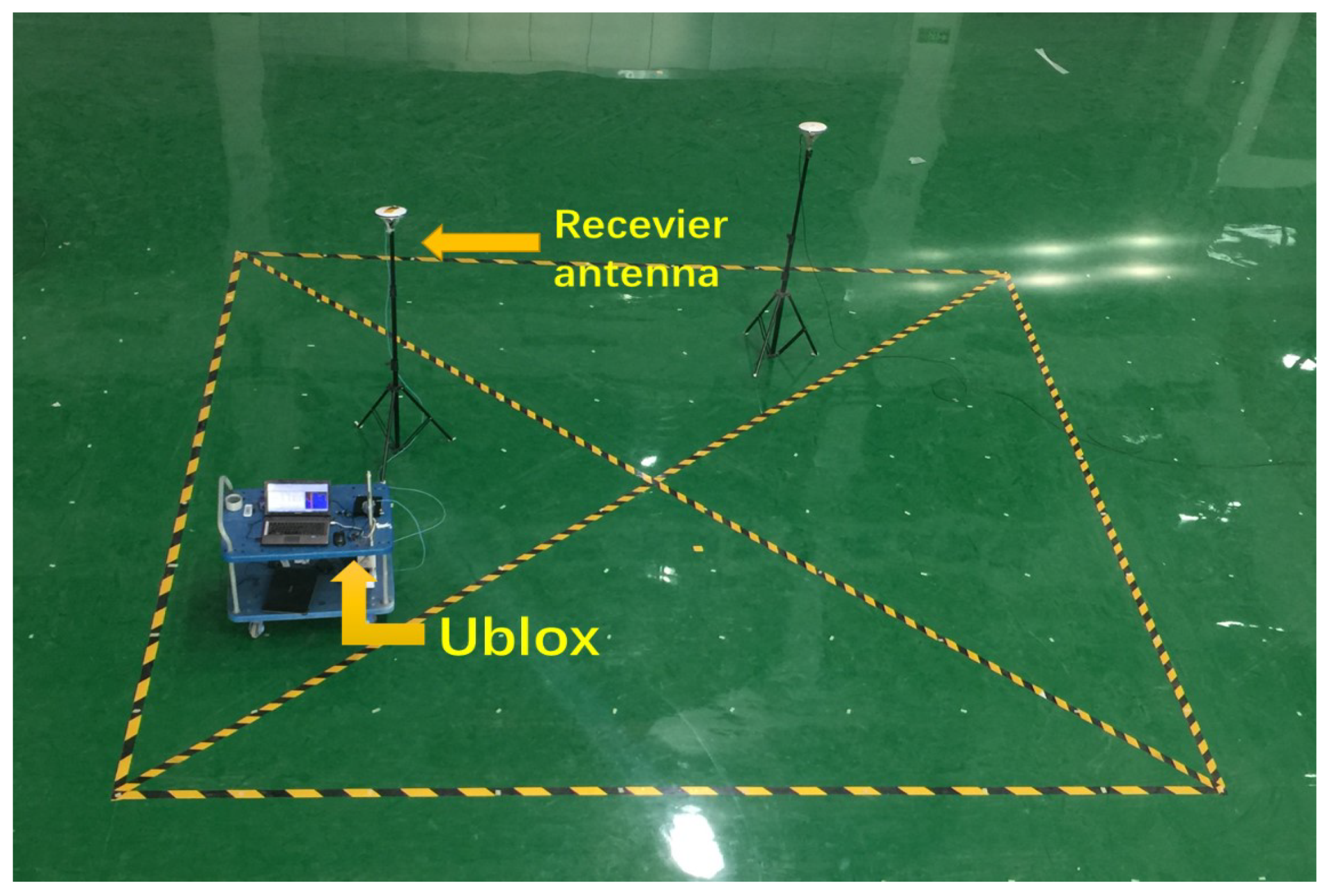
3.3. Actual Positioning Experiment

The ground navigation system consists of eight base stations, and each base station is regarded as a pseudolite. The system is installed in a 15 m ∗ 15 m room, as shown in Figure 7. We conducted a static test at a known location (the “receiver” in Figure 7) to evaluate the pseudolite signal quality and indoor positioning accuracy. The receiver includes the receiving antenna and the Ublox module connected to the computer. The receiving point location is far from the wall, and there are no other obstacles around, which can help the receiver reduce the impact of multipath. Then, we used the receiver to collect carrier phase and pseudorange data.

The signal transmission baseband unit of the pseudolite is a multi-channel RF module (ad9371) driven by FPGA and DSP. Each station can transmit an L1 (1575.42 MHz) signal, and each base station includes an antenna. All transceivers share a common clock source for time synchronization. Pseudolites are installed on the top of the house, on the same horizontal plane, and the maximum height difference is within 1.5 cm. In order to make the signal strength of the pseudolites received high and reduce the influence of multipath, we put the pseudolites at a high position and keep the distance between the pseudolites to avoid signal interference. We used an Electronic Total Station for antennas of transceivers coordinates determination, and the calibration accuracy is 1–2 mm. We used a relative coordinate system, where a particular position in the room is the origin of the coordinates, and other coordinates are the relative positions from this point. We plot the coordinate distribution of pseudolites as shown in Figure 8. The coordinates of the pseudolites are shown in

Table 4. Position distribution of pseudolites.

Pseudolite	X (m)	Y (m)	Z (m)
1	3.5659	−1.8707	11.3553
2	−2.8797	−2.2747	11.3568
3	−5.2303	0.464	11.3562
4	−5.6214	7.344	11.3456
5	−3.3354	9.1587	11.3428
6	2.6414	9.5559	11.3459
7	5.098	8.0073	11.3476
8	5.5518	1.1654	11.3507

.

4. Experiments by Indoor Navigation System

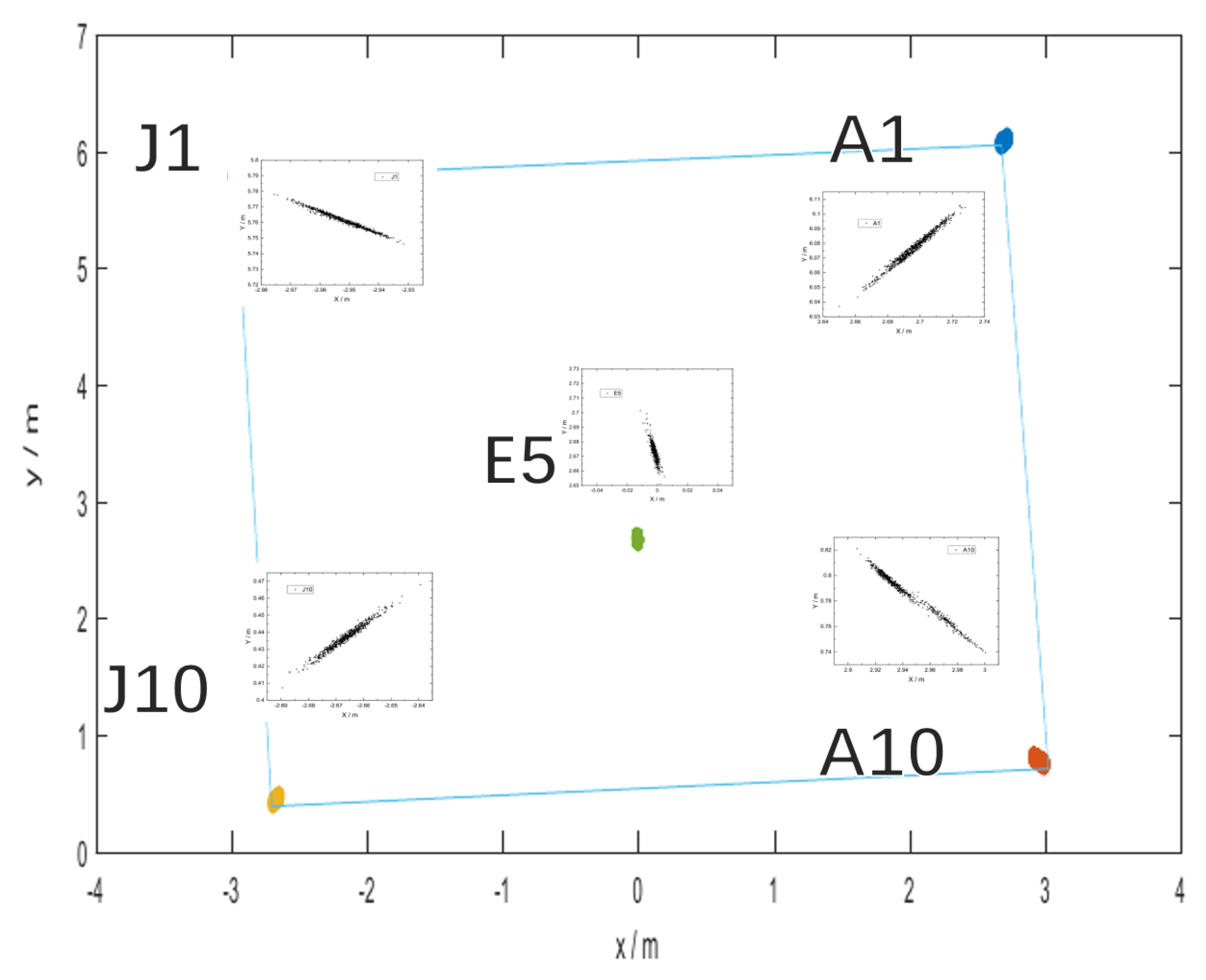
4.1. Static Point Positioning

We use the KPI positioning method proposed in Reference [20] and use carrier phase observations to obtain positioning results. Using carrier phase for static point positioning can reduce the influence of multipath and obtain centimeter-level positioning solutions. We performed static positioning at the corner and center of the positioning area, as shown in Figure 9. The relative height value of all test points is 0.35 m.

It can be analyzed from Figure 9 that, when the positioning point is closer to the corner, the value of WHDOP is larger the result of static positioning is more scattered, and shows a linear distribution. Conversely, when the position of the receiver is close to the center, the value of WHDOP is smaller, and the positioning result shows a tendency to cluster. Then, we tested the positioning of the other three corners and plotted the positioning results, as shown in Figure 10. In the other three corners, the coordinates are A10 (3.0223, 0.7152), J1 (−2.9701, 5.7737), and J10 (−2.7025, 0.3928) shows the same trend as A1, that is, a linear positioning error.

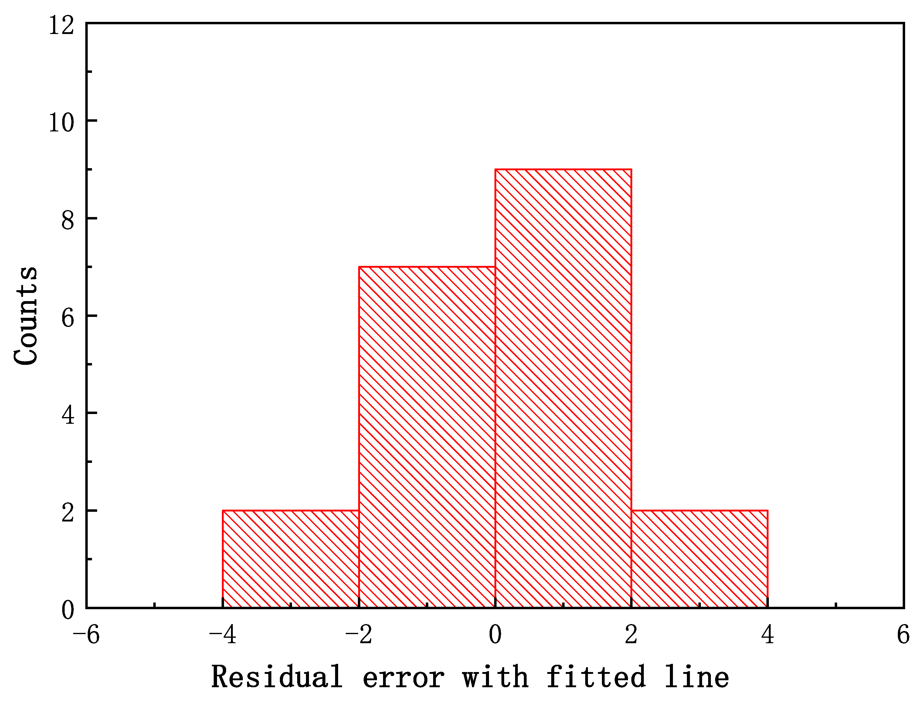
4.2. Pearson Correlation Coefficient Verification

We carried out the Pearson correlation coefficient between WHDOP and the positioning result to verify that the proposed WHDOP method has practical application significance. Pearson product-moment correlation coefficient (PPMCC), also called Pearson correlation coefficient (PCC for short), is used to measure the correlation (linear correlation) between two variables, X and Y. In statistics, its value is between −1 and 1. The larger the absolute value of the correlation coefficient presents, the stronger the correlation between the two sets of data. If one variable increases, the other variable also increases, indicating a positive correlation between them, and the correlation coefficient is greater than 0. If one variable increases, the other variable decreases, indicating a negative correlation between them, and the correlation coefficient is less than 0. When the correlation coefficient is closer to 1 or −1, the correlation is vital. On the contrary, when the correlation coefficient is closer to 0, the correlation is weaker. The Pearson correlation coefficient between two sets of data is defined as the covariance and standard deviation quotient. The calculation equation is as follows:

$$r=\frac{cov(X,Y)}{{\sigma }_X{\sigma }_Y},$$

(34)

$$r=\frac{{\sum }_{i=1}^n(X_i-\overline{X})(Y_i-\overline{Y})}{\sqrt{{\sum }_{i=1}^n{(X_i-\overline{X})}^2}\sqrt{{\sum }_{i=1}^n{(Y_i-\overline{Y})}^2}},$$

(35)

where X and Y are the averages of the two sets of data. We randomly selected 20 positioning points and calculated the positioning variance and WHDOP of each positioning point. Among the twenty points, the static positioning variance of 19 points is within 1.2 cm, and the positioning variance of only one point is 1.5 cm. This shows that the positioning system can reach centimeter-level or even sub-centimeter-level positioning accuracy. According to the Equation (35), the correlation coefficient of these points is calculated to be 0.82, which proves that the positioning error has a linear relationship with our proposed WHDOP. We performed a linear fit according to the minimum residual sum, as shown in Figure 11.

Most of the points are distributed to the straight line, and a few points deviate from the straight line, which can be seen from the Figure 11. The sum of squared residuals is 64 (mm${}^2$). In order to analyze the result, a histogram of the residual result points is marked as shown in Figure 12.

5. Discussion and Conclusions

Unlike GNSS, indoor positioning focuses on horizontal positioning accuracy. We proposed a new method for evaluating horizontal positioning accuracy, called WHDOP. In addition to the horizontal precision factor, as in the traditional method, the pseudolite signal strength factor received by the receiver is also included in WHDOP, which can reflect the accurate positioning accuracy. Then, based on the traditional inversion operation, this study provided yet another method to compute WHDOP. The distance between base stations is also taken into account in the deployment constraints to meet the need for time synchronisation between base stations in wireless systems. A practical example is used to illustrate the calculation process of the proposed WHDOP, which can reduce the amount of calculation during the pseudolites layout search process. In contrast to the conventional simulation approach, real ground-based navigation which can realize centimeter-level positioning precision was built up for tests. Eight pseudolites were used for testing and the distribution of the pseudolites was accurately measured. Within the positioning area, grid points were divided for positioning sampling, and their respective WHDOP values and positioning standard deviations were calculated. We used actual test examples to verify the practical application significance of the proposed WHDOP. The correlation coefficient between 20 randomly selected static test results, which shows a strong linear relationship between the WHDOP value and the positioning accuracy. This proves the superiority of our proposed method. Based on WHDOP, a particle swarm algorithm based on a simulated annealing algorithm is proposed to search for the position of pseudolites. The accuracy of the method are proved by the simulation experiments.

References

1. Chao, M.; Wang, J.; Chen, J. Beidou compatible indoor positioning system architecture design and research on geometry of pseudolite. In Proceedings of the 2016 Fourth International Conference on Ubiquitous Positioning, Indoor Navigation and Location Based Services (UPINLBS), Shanghai, China, 9 January 2017; pp. 176–181. [Google Scholar]
2. Chen, Y.; Francisco, J.-A.; Trappe, W.; Martin, R.P. A practical approach to landmark deployment for indoor localization. In Proceedings of the 2006 3rd Annual IEEE Communications Society on Sensor and Ad Hoc Communications and Networks, Reston, VA, USA, 28–28 September 2006; Volume 1, pp. 365–373. [Google Scholar]
3. Ma, C.; Yang, J.; Chen, J.; Tang, Y. Indoor and outdoor positioning system based on navigation signal simulator and pseudolites. Adv. Space Res. 2018, 62, 2509–2517. [Google Scholar] [CrossRef]
4. Guo, X.; Zhou, Y.; Wang, J.; Liu, K.; Liu, C. Precise point positioning for ground-based navigation systems without accurate time synchronization. GPS Solut. 2018, 22, 34. [Google Scholar] [CrossRef]
5. Cobb, S.; Lawrence, D.; Pervan, B.; Cohen, C.; Powell, D.; Parkinson, B. Precision landing tests with improved integrity beacon pseudolites. Proc. ION GPS 1995, 8, 827–833. [Google Scholar]
6. Montillet, J.P.; Roberts, G.W.; Hancock, C.; Meng, X.; Ogundipe, O.; Barnes, J. Deploying a Locata network to enable precise positioning in urban canyons. J. Geod. 2009, 83, 91–103. [Google Scholar] [CrossRef]
7. Wang, T.; Yao, Z.; Lu, M. On-the-fly ambiguity resolution involving only carrier phase measurements for stand-alone ground-based positioning systems. GPS Solut. 2019, 23, 36. [Google Scholar] [CrossRef]
8. Sairo, H.; Akopian, D.; Takala, J. Weighted dilution of precision as quality measure in satellite positioning. IEE Proc.-Radar Sonar Navig. 2003, 150, 430–436. [Google Scholar] [CrossRef]
9. Shing, H.; Doong, A. Closed-form equation for GPS GDOP computation. GPS Solut. 2009, 13, 183–190. [Google Scholar]
10. Jwo, D.; Lai, C. Neural network-based GPS GDOP approximation and classification. GPS Solut. 2007, 13, 51–60. [Google Scholar] [CrossRef]
11. Zhu, J. Calculation of geometric dilution of precision. IEEE Trans. Aerosp. Elect. Syst. 1992, 28, 893–894. [Google Scholar]
12. Yarlagadda, R.; Ali, I.; Al-Dhahir, N.; Hershey, J. GPS GDOP metric. IEE Proc. Radar Sonar Navig. 2000, 147, 259–264. [Google Scholar] [CrossRef]
13. Sun, Y.; Wang, J.; Chen, J. Indoor precise point positioning with pseudolites using estimated time biases iPPP and iPPP-RTK. GPS Solut. 2021, 25, 41. [Google Scholar] [CrossRef]
14. Wang, T.; Yao, Z.; Lu, M. Combined difference square observation-based ambiguity determination for ground-based positioning system. J. Geod. 2019, 93, 1867–1880. [Google Scholar] [CrossRef]
15. Hu, W.; Yang, J.J.; He, P. Study on Pseudolite Configuration Scheme Based on Near Space Airships. Radio Eng. 2009, 39, 10. [Google Scholar]
16. Yi, Y.; She-sheng, G.; Hai-feng, Y. Design on geometric configuration schemes of pseudolite in near space. Syst. Eng. Electron. 2014, 36, 3. [Google Scholar]
17. Simon, D.; El-Sherief, H. Navigation satellite selection using neural networks. Neurocomputing 1995, 7, 247–258. [Google Scholar] [CrossRef] [Green Version]
18. Hager, W.W. Updating the inverse of a matrix. SIAM Rev. 1989, 31, 221–239. [Google Scholar] [CrossRef]
19. Shi, Y.H.; Eberhart, R. A Modified Particle Swarm Optimizer. In Proceedings of the IEEE Conference on Evolutionary Computation, Anchorage, AK, USA, 4–9 May 1998; pp. 69–73. [Google Scholar]
20. Barnes, J.; Rizos, C.; Wang, J.; Small, D.; Voigt, G.; Gambale, N. Locata: A new positioning technology for high precision indoor and outdoor positioning. In Proceedings of the 2003 International Symposium on GPS, Tokyo, Japan, 15–18 November 2003; pp. 9–18. [Google Scholar]
21. Hoffman, K.; Kunze, R.A. Linear Algebra; Prentice-Hall: Englewood Cliffs, NJ, USA, 1961. [Google Scholar]
22. Santerre, R.; Geiger, A.; Banville, S. Geometry of GPS dilution of precision: Revisited. GPS Solut. 2017, 21, 1747–1763. [Google Scholar] [CrossRef]
23. Chen, C. Weighted Geometric Dilution of Precision Calculations with Matrix Multiplication. Sensors 2015, 15, 803–817. [Google Scholar] [CrossRef]
24. Pan, L.; Cai, C.; Santerre, R.; Zhang, X. Performance evaluation of single-frequency point positioning with GPS, GLONASS, Beidou and Galileo. Surv. Rev. 2016, 49, 197–205. [Google Scholar] [CrossRef]
25. Metropolis, N.; Ulam, S. The monte carlo method. J. Am. Stat. Assoc. 1949, 44, 335–341. [Google Scholar] [CrossRef]
26. Bernstein, D.J. Understanding Brute Force. 2005. Available online: http://citeseerx.ist.psu.edu/viewdoc/download?doi=10.1.1.139.4510&rep=rep1&type=pdf (accessed on 11 September 2021).
Figure 1. Six pseudolites and positioning points.
Ijgi 10 00601 g001
Figure 2. The value of WHDOP under six pseudolites by two different calculation methods.
Ijgi 10 00601 g002
Figure 3. Correspondence between iterative process and F value.
Ijgi 10 00601 g003
Figure 4. Comparison of the results of brute force search (top) and the proposed algorithm (bottom).
Ijgi 10 00601 g004
Figure 5. WHDOP distribution map of 6 pseudolites.
Ijgi 10 00601 g005
Figure 6. WHDOP distribution map of 8 pseudolites.
Ijgi 10 00601 g006
Figure 7. Ground-based navigation system receiving module.
Ijgi 10 00601 g007
Figure 8. Pseudolite position distribution.
Ijgi 10 00601 g008
Figure 9. (top) The positioning result of the static point A1 (2.6777, 6.059); (bottom) the positioning result of the static point E5 (0, 2.6734).
Ijgi 10 00601 g009
Figure 10. Positioning results in the four corners and central area of the positioning area.
Ijgi 10 00601 g010
Figure 11. WHDOP and positioning residual fitting line.
Ijgi 10 00601 g011
Figure 12. Residual distance and quantity statistics chart.
Ijgi 10 00601 g012