
How Did Built Environment Affect Urban Vitality in Urban Waterfronts? A Case Study in Nanjing Reach of Yangtze River


Abstract
:1. Introduction
2. Literature Review
2.1. The Measurements of Urban Vitality
2.2. The Relationship between Built Environment and Urban Vitality
3. Data and Methods
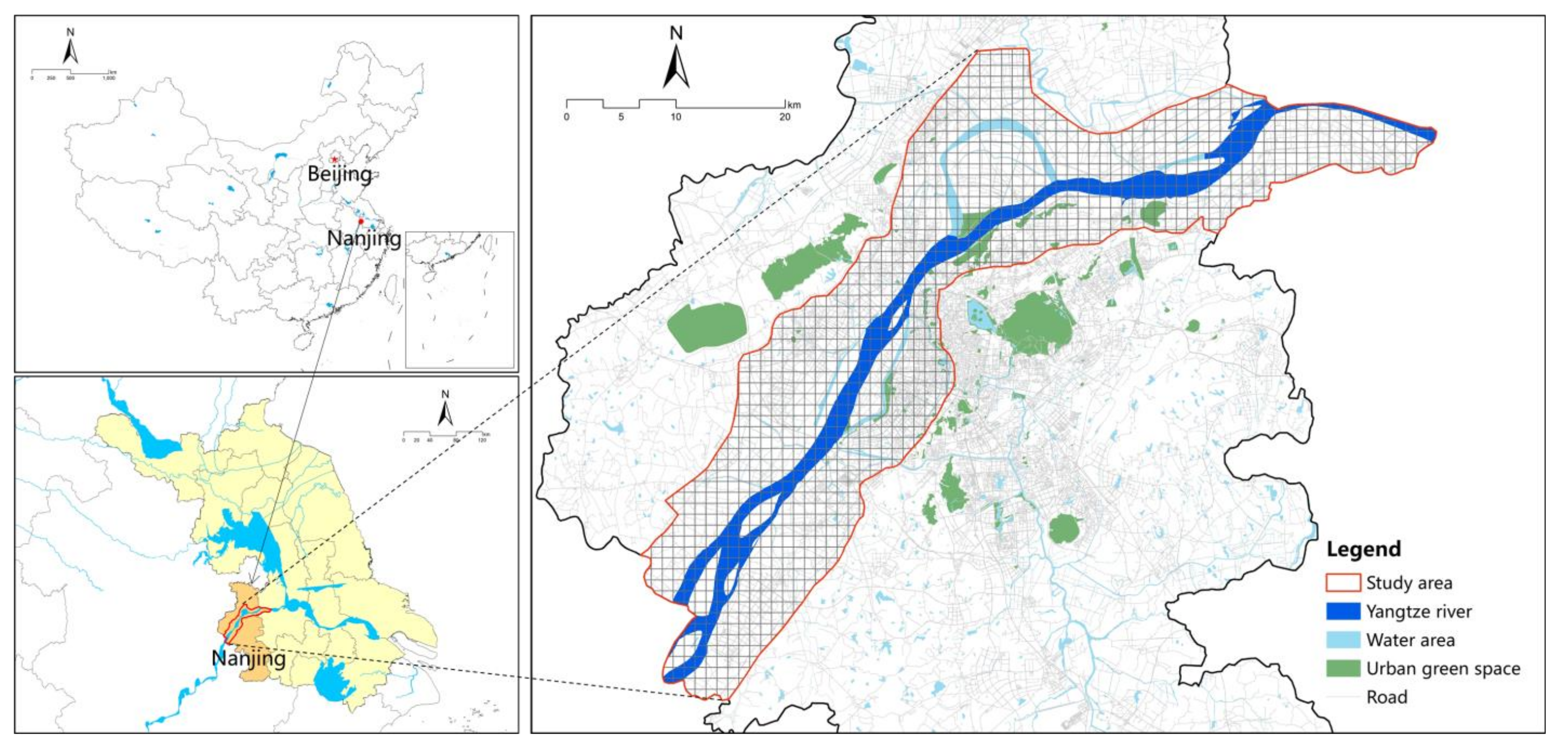
3.1. Study Area
3.2. Data
3.2.1. BHM Data
3.2.2. Other Complementary Data
3.3. Methods
3.3.1. Evaluating Urban Vitality in Urban Waterfronts
3.3.2. Associated Built Environment Variables
3.3.3. Global and Local Regression Models
4. Results
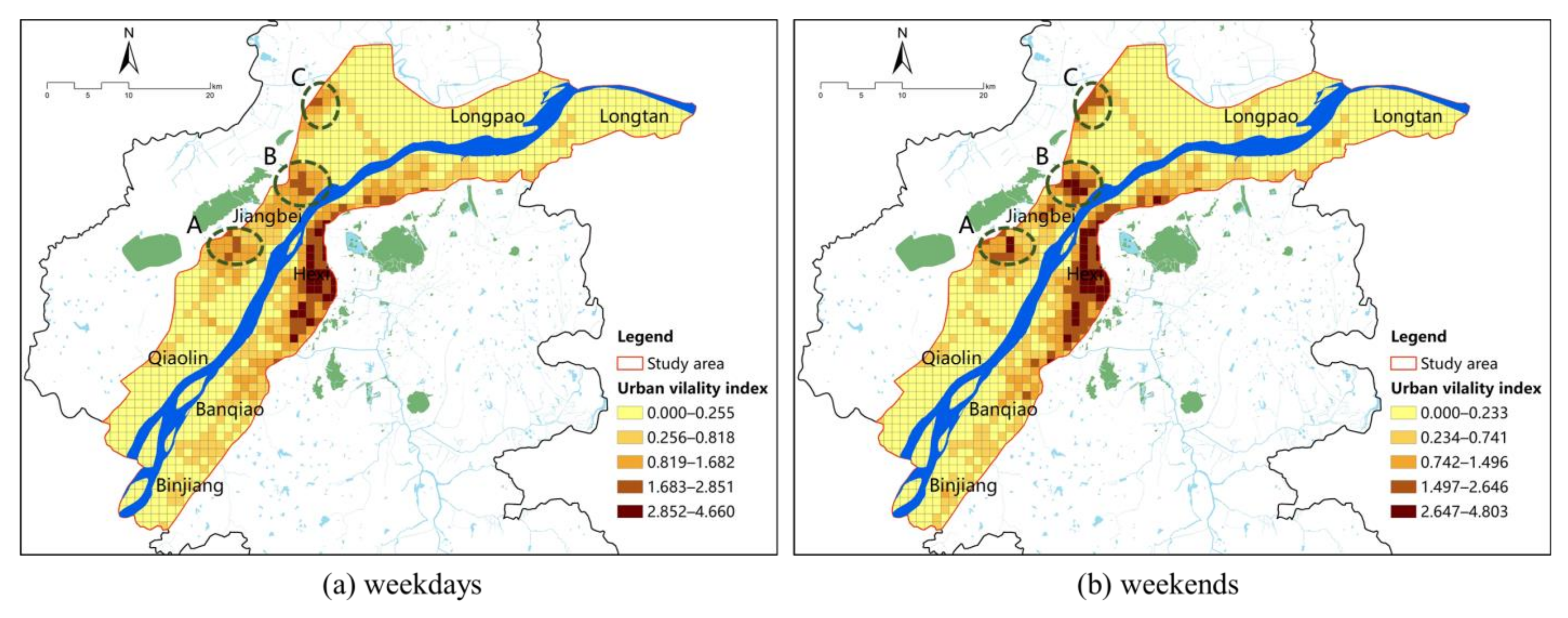
4.1. Characteristics of Urban Vitality in Urban Waterfronts
4.2. OLS Regression Analysis and Global Relationships
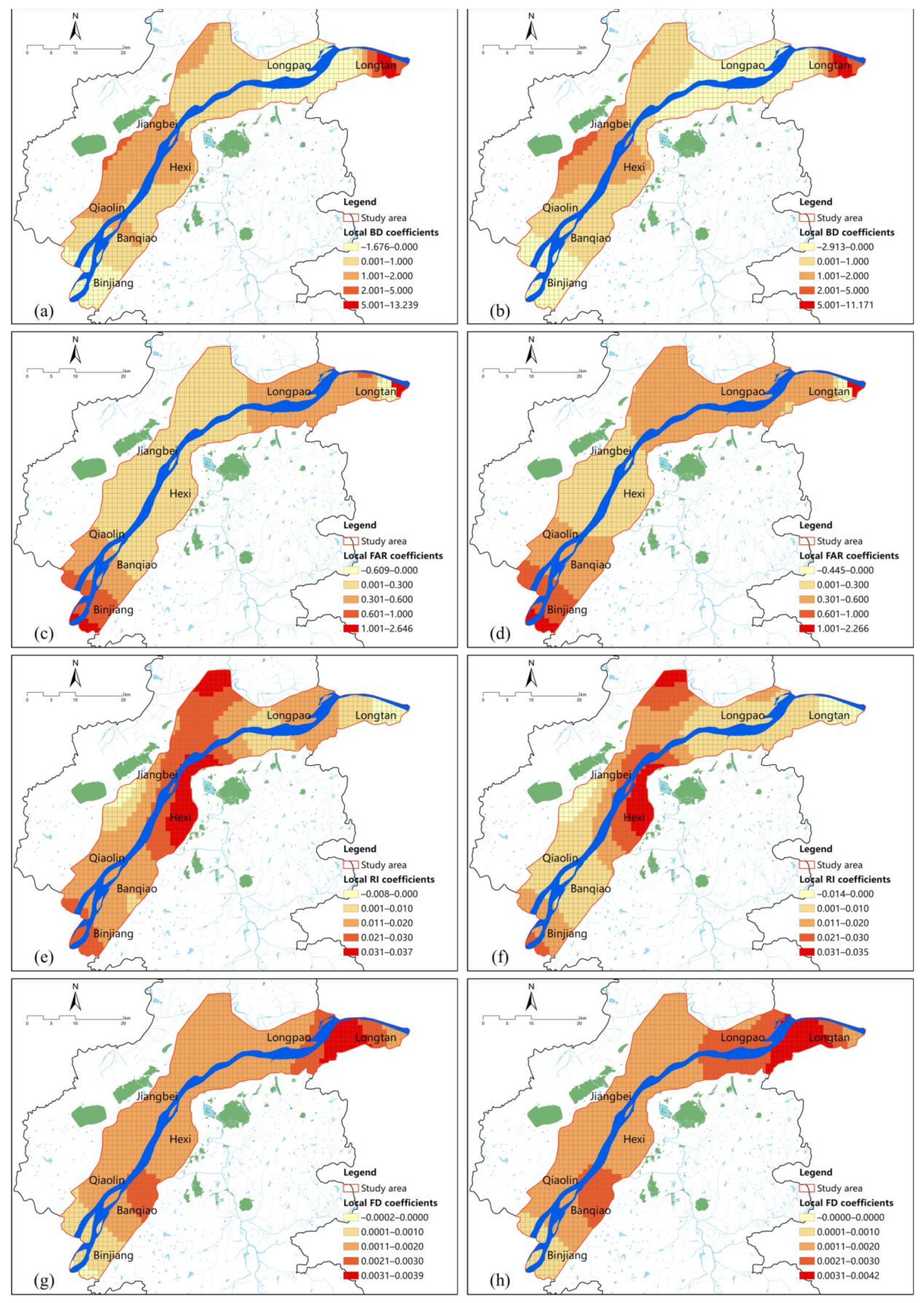
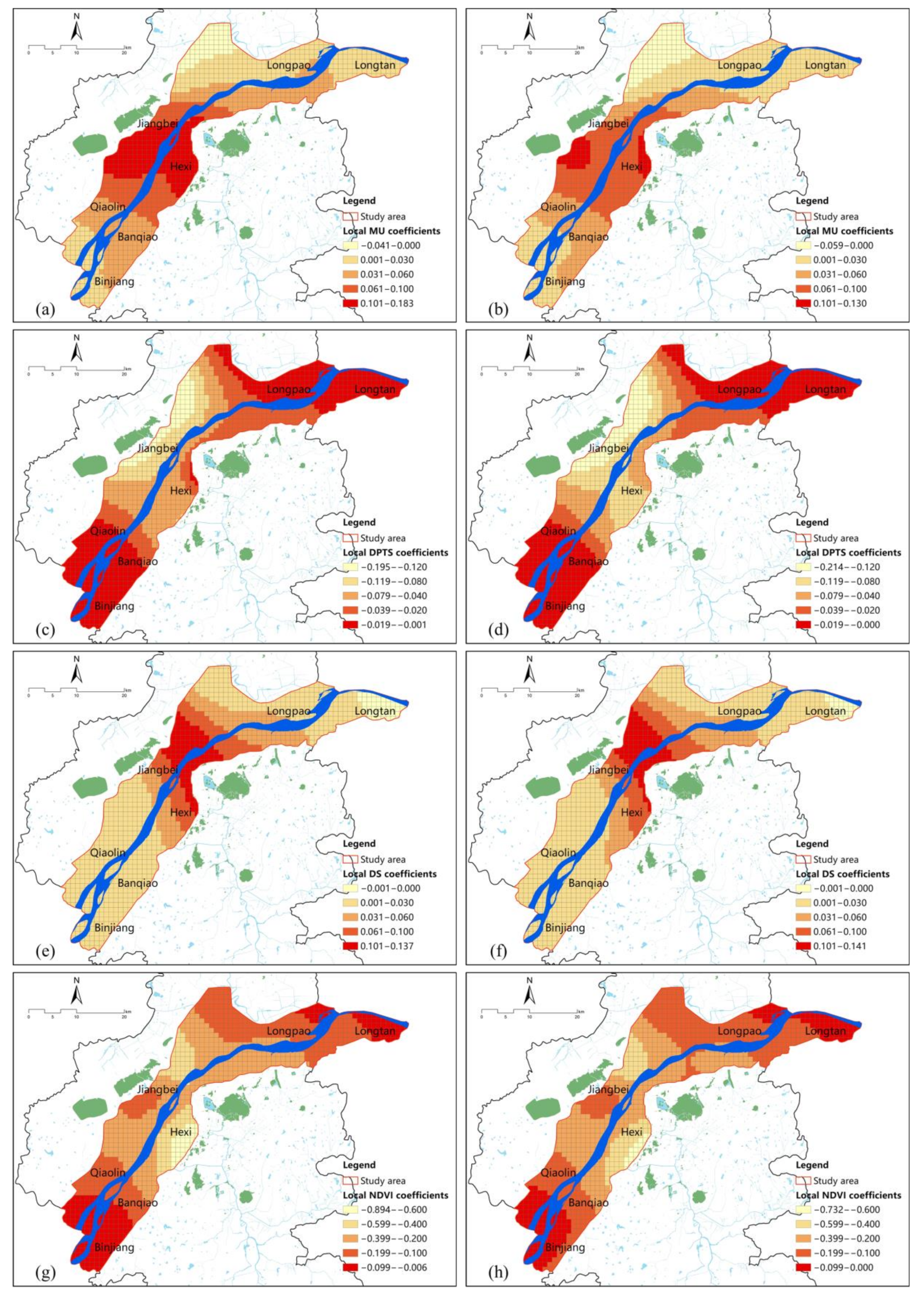
4.3. GWR Analysis and Spatial Variations
5. Discussion
5.1. Towards Establishing a BHM Data-Based Method for Assessing Urban Vitality in Urban Waterfronts
5.2. The Influencing of Built Environment Characteristics on Urban Vitality in Urban Waterfronts
5.3. Limitations and Future Studies
6. Conclusions
Author Contributions
Funding
Institutional Review Board Statement
Informed Consent Statement
Data Availability Statement
Acknowledgments
Conflicts of Interest
References
- Kostopoulou, S. On the revitalized waterfront: Creative milieu for creative tourism. Sustainability 2013, 5, 4578–4593. [Google Scholar] [CrossRef] [Green Version]
- Hoyle, B. Urban waterfront revitalization in developing countries: The example of Zanzibar’s Stone Town. Geogr. J. 2002, 168, 141–162. [Google Scholar] [CrossRef]
- Keyvanfar, A.; Shafaghat, A.; Mohamad, S.; Abdullahi, M.a.M.; Ahmad, H.; Mohd Derus, N.H.; Khorami, M. A Sustainable Historic Waterfront Revitalization Decision Support Tool for Attracting Tourists. Sustainability 2018, 10, 215. [Google Scholar] [CrossRef] [Green Version]
- Ma, Y.; Ling, C.; Wu, J. Exploring the Spatial Distribution Characteristics of Emotions of Weibo Users in Wuhan Waterfront Based on Gender Differences Using Social Media Texts. ISPRS Int. J. Geo-Inf. 2020, 9, 465. [Google Scholar] [CrossRef]
- Hagerman, C. Shaping neighborhoods and nature: Urban political ecologies of urban waterfront transformations in Portland, Oregon. Cities 2007, 24, 285–297. [Google Scholar] [CrossRef]
- Girard, L.F.; Kourtit, K.; Nijkamp, P. Waterfront Areas as Hotspots of Sustainable and Creative Development of Cities. Sustainability 2014, 6, 4580–4586. [Google Scholar] [CrossRef] [Green Version]
- Shah, S.; Roy, A.K. Social sustainability of urban waterfront-the case of carter road waterfront in Mumbai, India. Procedia Environ. Sci. 2017, 37, 195–204. [Google Scholar] [CrossRef]
- Sairinen, R.; Kumpulainen, S. Assessing social impacts in urban waterfront regeneration. Environ. Impact Assess. Rev. 2006, 26, 120–135. [Google Scholar] [CrossRef]
- Avni, N.; Teschner, N.A. Urban Waterfronts: Contemporary Streams of Planning Conflicts. J. Plan. Lit. 2019, 34, 408–420. [Google Scholar] [CrossRef]
- Breen, A.; Rigby, D. The New Waterfront: A Worldwide Urban Success Story; Thames and Hudson: London, UK, 1996. [Google Scholar]
- Hoyle, B. Global and Local Change on the Port-City Waterfront. Geogr. Rev. 2000, 90, 395–417. [Google Scholar] [CrossRef]
- Cheung, D.M.-W.; Tang, B.-S. Social order, leisure, or tourist attraction? The changing planning missions for waterfront space in Hong Kong. Habitat Int. 2015, 47, 231–240. [Google Scholar] [CrossRef]
- Brownill, S. Just add water: Waterfront regeneration as a global phenomenon. In The Routledge Companion to Urban Regeneration; Leary, M.E., McCarthy, J., Eds.; Routledge: London, UK, 2013; pp. 45–55. [Google Scholar]
- Chang, T.C.; Huang, S. Reclaiming the City: Waterfront Development in Singapore. Urban Stud. 2010, 48, 2085–2100. [Google Scholar] [CrossRef]
- Gordon, D.L.A. Managing the changing political environment in urban waterfront redevelopment. Urban Stud. 1997, 34, 61–83. [Google Scholar] [CrossRef]
- Erbil, A.Ö.; Erbil, T. Redevelopment of Karaköy Harbor, Istanbul: Need for a new planning approach in the midst of change. Cities 2001, 18, 185–192. [Google Scholar] [CrossRef]
- Wang, J.; Lv, Z. A historic review of world urban waterfront development. City Plan. Rev. 2001, 25, 41–46. [Google Scholar]
- Liu, S.; Lai, S.-Q.; Liu, C.; Jiang, L. What influenced the vitality of the waterfront open space? A case study of Huangpu River in Shanghai, China. Cities 2021, 114, 103197. [Google Scholar] [CrossRef]
- Wu, J.; Li, J.; Ma, Y. A Comparative Study of Spatial and Temporal Preferences for Waterfronts in Wuhan based on Gender Differences in Check-In Behavior. ISPRS Int. J. Geo-Inf. 2019, 8, 413. [Google Scholar] [CrossRef] [Green Version]
- Jacobs, J. The Death and Life of Great American Cities; Vintage: New York, NY, USA, 1961. [Google Scholar]
- Lynch, K. Good City Form; MIT Press: Cambridge, MA, USA, 1984. [Google Scholar]
- Maas, P.R. Towards a Theory of Urban Vitality; The University of British Columbia: Vancouver, BC, Canada, 1984. [Google Scholar]
- Montgomery, J. Making a city: Urbanity, vitality and urban design. J. Urban Des. 1998, 3, 93–116. [Google Scholar] [CrossRef]
- Niu, H.; Silva, E.A. Crowdsourced Data Mining for Urban Activity: Review of Data Sources, Applications, and Methods. J. Urban Plan. Dev. 2020, 146, 04020007. [Google Scholar] [CrossRef] [Green Version]
- Wu, C.; Ye, X.; Ren, F.; Du, Q. Check-in behaviour and spatio-temporal vibrancy: An exploratory analysis in Shenzhen, China. Cities 2018, 77, 104–116. [Google Scholar] [CrossRef]
- Yue, Y.; Zhuang, Y.; Yeh, A.G.O.; Xie, J.-Y.; Ma, C.-L.; Li, Q.-Q. Measurements of POI-based mixed use and their relationships with neighbourhood vibrancy. Int. J. Geogr. Inform. Sci. 2016, 31, 658–675. [Google Scholar] [CrossRef] [Green Version]
- Wu, J.; Ta, N.; Song, Y.; Lin, J.; Chai, Y. Urban form breeds neighborhood vibrancy: A case study using a GPS-based activity survey in suburban Beijing. Cities 2018, 74, 100–108. [Google Scholar] [CrossRef]
- Kim, Y.-L. Seoul’s Wi-Fi hotspots: Wi-Fi access points as an indicator of urban vitality. Comput. Environ. Urban Syst. 2018, 72, 13–24. [Google Scholar] [CrossRef]
- Yang, J.; Cao, J.; Zhou, Y. Elaborating non-linear associations and synergies of subway access and land uses with urban vitality in Shenzhen. Transp. Res. Part A Policy Pract. 2021, 144, 74–88. [Google Scholar] [CrossRef]
- Long, Y.; Huang, C.C. Does block size matter? The impact of urban design on economic vitality for Chinese cities. Environ. Plan. B Urban Anal. City Sci. 2017, 46, 406–422. [Google Scholar] [CrossRef] [Green Version]
- Zhang, A.; Li, W.; Wu, J.; Lin, J.; Chu, J.; Xia, C. How can the urban landscape affect urban vitality at the street block level? A case study of 15 metropolises in China. Environ. Plan. B Urban Anal. City Sci. 2020, 48, 1245–1262. [Google Scholar] [CrossRef]
- Ye, Y.; Li, D.; Liu, X. How block density and typology affect urban vitality: An exploratory analysis in Shenzhen, China. Urban Geogr. 2018, 39, 631–652. [Google Scholar] [CrossRef]
- Huang, B.; Zhou, Y.; Li, Z.; Song, Y.; Cai, J.; Tu, W. Evaluating and characterizing urban vibrancy using spatial big data: Shanghai as a case study. Environ. Plan. B Urban Anal. City Sci. 2019, 47, 1543–1559. [Google Scholar] [CrossRef]
- Frank, L.D.; Engelke, P.O. The Built Environment and Human Activity Patterns: Exploring the Impacts of Urban Form on Public Health. J. Plan. Lit. 2001, 16, 202–218. [Google Scholar] [CrossRef]
- McAndrews, C.; Marshall, W. Livable Streets, Livable Arterials? Characteristics of Commercial Arterial Roads Associated with Neighborhood Livability. J. Am. Plan. Assoc. 2018, 84, 33–44. [Google Scholar] [CrossRef]
- Forsyth, A.; Hearst, M.; Oakes, J.M.; Schmitz, K.H. Design and Destinations: Factors Influencing Walking and Total Physical Activity. Urban Stud. 2008, 45, 1973–1996. [Google Scholar] [CrossRef]
- Mouratidis, K.; Poortinga, W. Built environment, urban vitality and social cohesion: Do vibrant neighborhoods foster strong communities? Landsc. Urban Plan. 2020, 204, 103951. [Google Scholar] [CrossRef]
- Xia, C.; Zhang, A.; Yeh, A.G.O. The Varying Relationships between Multidimensional Urban Form and Urban Vitality in Chinese Megacities: Insights from a Comparative Analysis. Ann. Am. Assoc. Geogr. 2021, 1–26. [Google Scholar] [CrossRef]
- Azmi, D.I.; Karim, H.A. Implications of Walkability Towards Promoting Sustainable Urban Neighbourhood. Procedia Soc. Behav. Sci. 2012, 50, 204–213. [Google Scholar] [CrossRef]
- Filion, P.; Hammond, K. Neighbourhood land use and performance: The evolution of neighbourhood morphology over the 20th century. Environ. Plan. B Plan. Des. 2003, 30, 271–296. [Google Scholar] [CrossRef]
- Tu, W.; Zhu, T.; Xia, J.; Zhou, Y.; Lai, Y.; Jiang, J.; Li, Q. Portraying the spatial dynamics of urban vibrancy using multisource urban big data. Comput. Environ. Urban Syst. 2020, 80, 101428. [Google Scholar] [CrossRef]
- Nadai, M.D.; Staiano, J.; Larcher, R.; Sebe, N.; Quercia, D.; Lepri, B. The Death and Life of Great Italian Cities: A Mobile Phone Data Perspective. In Proceedings of the 25th International Conference on World Wide Web, Montreal, QC, Canada, 11–15 April 2016. [Google Scholar]
- Fan, Z.; Duan, J.; Lu, Y.; Zou, W.; Lan, W. A geographical detector study on factors influencing urban park use in Nanjing, China. Urban For. Urban Green 2021, 59, 126996. [Google Scholar] [CrossRef]
- Tan, X.; Huang, D.; Zhao, X.; Yu, Y.; Leng, B.; Feng, L. Jobs housing balance based on Baidu thermodynamic diagram. J. Beijing Norm. Univ. Nat. Sci. 2016, 52, 622–627. [Google Scholar]
- Zhang, S.; Zhang, W.; Wang, Y.; Zhao, X.; Song, P.; Tian, G.; Mayer, A.L. Comparing Human Activity Density and Green Space Supply Using the Baidu Heat Map in Zhengzhou, China. Sustainability 2020, 12, 7075. [Google Scholar] [CrossRef]
- Lyu, F.; Zhang, L. Using multi-source big data to understand the factors affecting urban park use in Wuhan. Urban For. Urban Green 2019, 43, 126367. [Google Scholar] [CrossRef]
- Li, J.; Li, J.; Yuan, Y.; Li, G. Spatiotemporal distribution characteristics and mechanism analysis of urban population density: A case of Xi’an, Shaanxi, China. Cities 2019, 86, 62–70. [Google Scholar] [CrossRef]
- Feng, D.; Tu, L.; Sun, Z. Research on Population Spatiotemporal Aggregation Characteristics of a Small City: A Case Study on Shehong County Based on Baidu Heat Maps. Sustainability 2019, 11, 6276. [Google Scholar] [CrossRef] [Green Version]
- Wu, Z.; Ye, Z. Research on urban spatial structure based on Baidu heat map: A case study on the central city of Shanghai. City Plan. Rev. 2016, 40, 33–40. [Google Scholar]
- Gehl, J. Life Between Buildings: Using Public Space; Island Press: Washington, DC, USA, 1971. [Google Scholar]
- Salingaros, N.A. Complexity and Urban Coherence. J. Urban Des. 2000, 5, 291–316. [Google Scholar] [CrossRef]
- Alexander, C. The Nature of Order, Book Three: A Vision of A Living World: An Essay on the Art of Building and The Nature of the Universe; The Center for Environmental Structure: Berkeley, CA, USA, 2005. [Google Scholar]
- Jacobs-Crisioni, C.; Rietveld, P.; Koomen, E.; Tranos, E. Evaluating the Impact of Land-Use Density and Mix on Spatiotemporal Urban Activity Patterns: An Exploratory Study Using Mobile Phone Data. Environ. Plan. A Econ. Space 2014, 46, 2769–2785. [Google Scholar] [CrossRef]
- Sung, H.; Lee, S.; Cheon, S. Operationalizing jane jacobs’s urban design theory: Empirical verification from the great city of seoul, korea. J. Plan. Educ. Res. 2015, 35, 117–130. [Google Scholar] [CrossRef]
- Xia, C.; Yeh, A.G.-O.; Zhang, A. Analyzing spatial relationships between urban land use intensity and urban vitality at street block level: A case study of five Chinese megacities. Landsc. Urban Plan. 2020, 193, 103669. [Google Scholar] [CrossRef]
- Fotheringham, A.S.; Charlton, M.E.; Brunsdon, C. Geographically weighted regression: A natural evolution of the expansion method for spatial data analysis. Environ. Plan. A 1998, 30, 1905–1927. [Google Scholar] [CrossRef]
- Fotheringham, A.S.; Brunsdon, C. Local forms of spatial analysis. Geograph. Anal. 1999, 31, 340–358. [Google Scholar] [CrossRef]
- Su, S.; Lei, C.; Li, A.; Pi, J.; Cai, Z. Coverage inequality and quality of volunteered geographic features in Chinese cities: Analyzing the associated local characteristics using geographically weighted regression. Appl. Geogr. 2017, 78, 78–93. [Google Scholar] [CrossRef]
- Zhao, P.; Xu, Y.; Liu, X.; Kwan, M.-P. Space-time dynamics of cab drivers’ stay behaviors and their relationships with built environment characteristics. Cities 2020, 101, 102689. [Google Scholar] [CrossRef]
- Lin, Y.; Hu, X.; Zheng, X.; Hou, X.; Zhang, Z.; Zhou, X.; Qiu, R.; Lin, J. Spatial variations in the relationships between road network and landscape ecological risks in the highest forest coverage region of China. Ecol. Indic. 2019, 96, 392–403. [Google Scholar] [CrossRef]
- Li, C.; Li, F.; Wu, Z.; Cheng, J. Exploring spatially varying and scale-dependent relationships between soil contamination and landscape patterns using geographically weighted regression. Appl. Geogr. 2017, 82, 101–114. [Google Scholar] [CrossRef]
- Wang, Y.; Dong, L.; Liu, Y.; Huang, Z.; Liu, Y. Migration patterns in China extracted from mobile positioning data. Habitat Int. 2019, 86, 71–80. [Google Scholar] [CrossRef]
- Nanjing Planning Bureau. Nanjing Master Planning (2011–2020); Nanjing Planning Bureau: Nanjing, China, 2017. Available online: http://ghj.nanjing.gov.cn/ghbz/ztgh/201705/t20170509_874089.html (accessed on 25 August 2021).
- Fang, L.; Huang, J.; Zhang, Z.; Nitivattananon, V. Data-driven framework for delineating urban population dynamic patterns: Case study on Xiamen Island, China. Sustain. Cities Soc. 2020, 62, 102365. [Google Scholar] [CrossRef] [PubMed]
- Meng, Y.; Xing, H. Exploring the relationship between landscape characteristics and urban vibrancy: A case study using morphology and review data. Cities 2019, 95, 102389. [Google Scholar] [CrossRef]
- Tang, L.; Lin, Y.; Li, S.; Li, S.; Li, J.; Ren, F.; Wu, C. Exploring the Influence of Urban Form on Urban Vibrancy in Shenzhen Based on Mobile Phone Data. Sustainability 2018, 10, 4565. [Google Scholar] [CrossRef] [Green Version]
- Fotheringham, A.S.; Brunsdon, C.; Charlton, M. Geographically Weighted Regression: The Analysis of Spatially Varying Relationships; John Wiley & Sons: New York, NY, USA, 2003. [Google Scholar]
- Akaike, H. Likelihood of a model and information criteria. J. Econom. 1981, 16, 3–14. [Google Scholar] [CrossRef]
- Dovey, K.; Pafka, E. What is walkability? The urban DMA. Urban Stud. 2020, 57, 93–108. [Google Scholar] [CrossRef]
- Hartig, T.; Mitchell, R.; De Vries, S.; Frumkin, H. Nature and health. Annu. Rev. Public Health 2014, 35, 207–228. [Google Scholar] [CrossRef] [PubMed] [Green Version]
- Liu, S.; Zhang, L.; Long, Y.; Long, Y.; Xu, M. A New Urban Vitality Analysis and Evaluation Framework Based on Human Activity Modeling Using Multi-Source Big Data. ISPRS Int. J. Geo-Inf. 2020, 9, 617. [Google Scholar] [CrossRef]
- Cui, N.; Malleson, N.; Houlden, V.; Comber, A. Using VGI and Social Media Data to Understand Urban Green Space: A Narrative Literature Review. ISPRS Int. J. Geo-Inf. 2021, 10, 425. [Google Scholar] [CrossRef]
- Evans, G. Measure for Measure: Evaluating the Evidence of Culture’s Contribution to Regeneration. Urban Stud. 2005, 42, 959–983. [Google Scholar] [CrossRef]
- Wu, J.; Li, J.; Ma, Y. Exploring the Relationship between Potential and Actual of Urban Waterfront Spaces in Wuhan Based on Social Networks. Sustainability 2019, 11, 3298. [Google Scholar] [CrossRef] [Green Version]


| Dimensions | Variables | Abbr. | Descriptions | Data Source |
|---|---|---|---|---|
| Density | Building density | BD | The building density of each square kilometer grid | map.baidu.com (2020) |
| Floor area ratio | FAR | The floor area ratio of each square kilometer grid | map.baidu.com (2020) | |
| Road intersections | RI | The number of road intersections of each square kilometer grid | Open Street Map (2020) | |
| Functional density | FD | The number of POI of each square kilometer grid | map.baidu.com (2020) | |
| Diversity | Mixed use | MU | The Shannon entropy is used to calculate the mixed use [27,41], , where D is mixed use index, is the proportions of each of the POI types (residential POI, commercial POI, traffic POI, office POI, science, education and health POI, and green space and square POI), and is the number of the POI types, in this case = 6. | map.baidu.com (2020) |
| Accessibility | Distance to public transport stations | DPTS | The distance to the nearest bus or subway stations of each square kilometer grid | nanjing.gongjiao.com (2020) |
| Distance to shoreline | DS | The distance to the nearest shoreline of each square kilometer grid | Nanjing master planning (2011–2020) | |
| Vegetation | Normalized difference vegetation index | NDVI | The average value of NDVI of each square kilometer grid, , where denotes near-infrared band, and is the red band. | Landsat 8 OLI, spatial resolution 30 m × 30 m (2020) |
| Maximum | Minimum | Mean | Median | SD | |
|---|---|---|---|---|---|
| weekdays | 4.660 | 0.000 | 0.380 | 0.041 | 0.715 |
| weekends | 4.803 | 0.000 | 0.382 | 0.029 | 0.737 |
| Variable | Coefficient | t-Statistic | Std. | VIF |
|---|---|---|---|---|
| BD | 1.021 | 5.315 ** | 0.192 | 4.874 |
| FAR | 0.182 | 5.309 * | 0.034 | 5.784 |
| RI | 0.020 | 7.20 ** | 0.003 | 1.983 |
| FD | 0.002 | 29.812 ** | 0.000 | 3.085 |
| MU | 0.065 | 5.106 ** | 0.012 | 1.813 |
| DPTS | −0.014 | −1.484 ** | 0.009 | 1.447 |
| DS | 0.032 | 6.493 ** | 0.005 | 1.362 |
| NDVI | −0.290 | −3.717 ** | 0.078 | 1.383 |
| AICs = 346.960 | ||||
| Adjusted R2 = 0.850 | ||||
| Variable | Coefficients | t-Statistic | Std. | VIF |
|---|---|---|---|---|
| BD | 0.690 | 3.407 ** | 0.203 | 4.874 |
| FAR | 0.291 | 8.069 ** | 0.036 | 5.784 |
| RI | 0.015 | 5.143 ** | 0.003 | 1.983 |
| FD | 0.002 | 28.709 ** | 0.000 | 3.085 |
| MU | 0.053 | 3.993 ** | 0.013 | 1.813 |
| DPTS | −0.016 | −1.681 ** | 0.010 | 1.447 |
| DS | 0.033 | 6.309 ** | 0.005 | 1.362 |
| NDVI | −0.269 | −3.276 ** | 0.082 | 1.383 |
| AICs = 479.678 | ||||
| Adjusted R2 = 0.843 | ||||
| Variable | Mean | Std. | Min | Lower Quartile | Median | Upper Quartile | Max |
|---|---|---|---|---|---|---|---|
| BD | 0.734 | 1.564 | −1.676 | −0.065 | 0.761 | 1.104 | 13.239 |
| FAR | 0.322 | 0.308 | −0.609 | 0.194 | 0.539 | 1.084 | 2.646 |
| RI | 0.016 | 0.009 | −0.008 | 0.011 | 0.014 | 0.023 | 0.037 |
| FD | 0.002 | 0.001 | −0.000 | 0.001 | 0.002 | 0.002 | 0.004 |
| MU | 0.049 | 0.042 | −0.041 | 0.021 | 0.035 | 0.079 | 0.183 |
| DPTS | −0.040 | 0.040 | −0.195 | −0.059 | −0.025 | −0.010 | −0.001 |
| DS | 0.037 | 0.035 | −0.001 | 0.016 | 0.020 | 0.050 | 0.137 |
| NDVI | −0.223 | 0.149 | −0.894 | −0.281 | −0.188 | −0.114 | −0.006 |
| AICs = 111.032 | |||||||
| Adjusted R2 = 0.880 | |||||||
| Variable | Mean | Std. | Min | Lower Quartile | Median | Upper Quartile | Max |
|---|---|---|---|---|---|---|---|
| BD | 0.392 | 1.516 | −2.913 | −0.506 | 0.398 | 0.925 | 11.171 |
| FAR | 0.377 | 0.268 | −0.445 | 0.264 | 0.355 | 0.409 | 2.266 |
| RI | 0.012 | 0.010 | −0.014 | 0.006 | 0.009 | 0.018 | 0.035 |
| FD | 0.002 | 0.001 | 0.000 | 0.002 | 0.002 | 0.002 | 0.004 |
| MU | 0.030 | 0.035 | −0.059 | 0.017 | 0.030 | 0.065 | 0.130 |
| DPTS | −0.024 | 0.047 | −0.214 | −0.077 | −0.024 | −0.009 | −0.000 |
| DS | 0.038 | 0.034 | −0.001 | 0.017 | 0.026 | 0.048 | 0.141 |
| NDVI | −0.211 | 0.132 | −0.732 | −0.269 | −0.177 | −0.112 | −0.000 |
| AICs = 269.201 | |||||||
| Adjusted R2 = 0.871 | |||||||
Publisher’s Note: MDPI stays neutral with regard to jurisdictional claims in published maps and institutional affiliations. |
© 2021 by the authors. Licensee MDPI, Basel, Switzerland. This article is an open access article distributed under the terms and conditions of the Creative Commons Attribution (CC BY) license (https://creativecommons.org/licenses/by/4.0/).
Share and Cite
Fan, Z.; Duan, J.; Luo, M.; Zhan, H.; Liu, M.; Peng, W. How Did Built Environment Affect Urban Vitality in Urban Waterfronts? A Case Study in Nanjing Reach of Yangtze River. ISPRS Int. J. Geo-Inf. 2021, 10, 611. https://0-doi-org.brum.beds.ac.uk/10.3390/ijgi10090611
Fan Z, Duan J, Luo M, Zhan H, Liu M, Peng W. How Did Built Environment Affect Urban Vitality in Urban Waterfronts? A Case Study in Nanjing Reach of Yangtze River. ISPRS International Journal of Geo-Information. 2021; 10(9):611. https://0-doi-org.brum.beds.ac.uk/10.3390/ijgi10090611
Chicago/Turabian StyleFan, Zhengxi, Jin Duan, Menglin Luo, Huanran Zhan, Mengru Liu, and Wangchongyu Peng. 2021. "How Did Built Environment Affect Urban Vitality in Urban Waterfronts? A Case Study in Nanjing Reach of Yangtze River" ISPRS International Journal of Geo-Information 10, no. 9: 611. https://0-doi-org.brum.beds.ac.uk/10.3390/ijgi10090611