
Influence of Relief Degree of Land Surface on Street Network Complexity in China


1
School of Geography and Information Engineering, China University of Geosciences, Wuhan 430078, China
2
College of Urban and Environmental Science, Central China Normal University, Wuhan 430079, China
*
Author to whom correspondence should be addressed.
ISPRS Int. J. Geo-Inf. 2021, 10(10), 705; https://0-doi-org.brum.beds.ac.uk/10.3390/ijgi10100705
Submission received: 9 June 2021
/
Revised: 6 October 2021
/
Accepted: 11 October 2021
/
Published: 15 October 2021
/
Corrected: 11 January 2022
Abstract
:The relief degree of land surface (RDLS) was often calculated to describe the topographic features of a region. It is a significant factor in designing urban street networks. However, existing studies do not clarify how RDLS affects the distribution of urban street networks. We used a Python package named OSMnx to extract the street networks of different cities in China. The street complexity metrics information (i.e., street grain, connectedness, circuity, and street network orientation entropy) were obtained and analyzed statistically. The results indicate that street network exhibits more complexity in regions with high RDLS. Further analysis of the correlation between RDLS and street network complexity metrics indicates that RDLS presents the highest correlation with street network circuity; that is, when RDLS is higher, the routes of an urban street network is more tortuous, and the additional travel costs for urban residents is higher. This study enriches and expands research on street networks in China, providing a reference value for urban street network planning.
1. Introduction
Urban planning defines the development and construction of a city. On the basis of the principles of sustainable development, it investigates the future development of a city and rationalizes its layout [1,2]. As one of the largest urban public spaces, an urban street network is the skeleton of the urban surface, presenting social and humanitarian connotations and becoming the focus in urban planning. It plays an important role in the physical/material and informational exchange of a city with its function of connecting one area to another [3].
As cities enter the period of spatial expansion into structural optimization, the scale of the street network gradually expands [4,5,6], and the rational planning of street structures becomes increasingly significant. Topographic information provides valuable support to various urban activities, such as urban waterlogging monitoring and urban expansion planning. Viero et al. pointed out that urban waterlogging was influenced by the natural environment, including precipitation and topography, so understanding urban topography is beneficial for monitoring urban waterlogging [7]. Yang et al. planned the road construction in the Jianye District of Nanjing by using topographic information, which effectively expressed the spatial geometry and semantic features of urban roads [8]. The close relationship between topographic information and streets may be valuable in the planning of urban streets [9], because of the combination of natural factors and human activities resulting in flat topography interspersed with undulating topography [10]. Many studies have demonstrated that topography has become a non-negligible factor in street network planning. For example, Osama et al. identified street network connectivity and topography as factors affecting pedestrian safety and found that higher continuity, linearity, coverage, and slope of the street network were associated with lower crash incidence, which was useful for street network planning [11]. Daniels et al. illustrated how the natural environment (including topography) influenced network planning principles through an analysis of the Sydney, Australia, case [12]. Szajowski et al. proposed a quantitative approach to measure the importance of roads based on topography and traffic intensity, which could be a guide for road builders planning road infrastructure [13].
Regional topographic features are typically identified by using the relief degree of land surface (RDLS) as a key indicator to characterize topographic relief in a certain area [14]. RDLS is frequently used as one of the indicators of habitat suitability evaluation [15] and ecological environment evaluation [16]. It is also widely used in the fields of geological disaster evaluation [17], soil erosion sensitivity evaluation [18], and population distribution and economic development [19]. An urban street network is the basic skeleton of urban spatial form that expresses evident complexity in many aspects, including topology structure [20]. At present, it is mostly described as a topological diagram. Thereafter, mathematical models are built and metrics are calculated for urban street networks, including the alpha index, the beta index, and the gamma index [21]. These metrics provide a good description of the structural characteristics of an urban street network. Most studies on urban street network complexity have selected a single city or a smaller scale of an area as objects of study. However, a small spatial scale usually reflects only the partial/individual characteristics of an area but not its overall/common characteristics embedded into the transportation network at a larger scale. Moreover, existing studies are typically limited to applying complex network theory [22], fractal theory [23], and space syntax [24] when measuring urban street network complexity.
Boeing proposed a street network complexity analysis method based on OSMnx, a Python package developed by his team [25]. This approach used a unified OpenStreetMap data source and optimized network topology. Street networks are complex research objects; hence, the introduction of OSMnx solves the following problems, which existed in previous studies on street networks: (1) network oversimplification and the inconsistency of simplified models exert fundamental effects on the research results [26], and (2) the lack of free downloadable and easy-to-handle tools [27]. OSMnx enables the measurement of urban street network complexity through street grain, connectedness, street network orientation entropy, and circuity. In recent years, some studies on urban street networks have been conducted by using OSMnx. Yen et al. used circuity as one of the metrics to analyze three street network patterns, namely, walkable, bikeable, and drivable, in Phnom Penh, Cambodia [28]. Their results suggested that urban central areas are more favorable for walking and biking than peripheral districts. Boeing used OSMnx as a data-access tool and the street network of 100 cities as the study subject. He included street orientation entropy as a metric for quantifying street network analysis and found that US cities tended to be more grid-oriented than other cities [29]. Moreover, the large sample of an urban street network can be collected by using OSMnx, considerably facilitating the study of urban street networks. Zhao et al. compared the network characteristics of the 26 pilot cities of the ASEAN Smart City Network by downloading the drivable and walkable road networks, using OSMnx with various network metrics [30]. Boeing used OSMnx and OpenStreetMap to analyze a street network with 27,000 urban street networks in the US and shared the large-scale data he collected in a public database [31]. Zhou et al. obtained a large sample of street network patterns by using OSMnx and found that similar street network patterns exhibit a clustered form in spatial distribution [32].
The influence of topography on a street network is one of the most important indicators of transportation costs and vehicle driving performance [33,34]. Nevertheless, existing studies have not yet explored in detail how topography affects the distribution of street networks. In our study, we used OSMnx to extract the city street networks of China and quantitatively analyze the closeness of the relationship between topography and street networks by the Pearson correlation coefficient. This study enriches and complements current research on the complexity of Chinese street networks in the theoretical and applied aspects. It contributes to the understanding of the layout and development of street network patterns and their associated urban forms in China, and may also play a greater role in future urban planning.
2. Study Area and Data
2.1. Overview of Study Area
In this study, China was chosen as the study area for the following reasons. First of all, Chinese territory is vast and shows great diversity in physical geography. For instance, the topography of China is high in the west and low in the east, and is complex and diverse, forming three levels of steps from west to east: The western part of the country has the highest terrain, the Qinghai-Tibet Plateau, known as the “Roof of the World”, which is the first step, and is bounded by the Kunlun Mountains, Qilian Mountains, Hengduan Mountains and the second step; the Qinghai-Tibet Plateau east to the Daxinganling Mountains, Taihang Mountains, Wushan Mountains and Xuefeng Mountains is the second step, generally at an altitude of 1000–2000 m, mainly composed of mountains, plateaus and basins; the wide plains and hills of eastern China are the third step. Secondly, the street system has developed significantly with the growth of cities since the implementation of China’s reform and open policy [35], but few studies have described the street network patterns of Chinese cities as a whole. Thirdly, with over 300 prefectures in China, it greatly helps us to explore whether the pattern of China’s street network is limited by the topography at a macro level.
2.2. Data
The digital elevation model (DEM) data used in our study were obtained from the Geospatial Data Cloud Platform (http://www.gscloud.cn (accessed on 5 March 2021)), with an accuracy of 30 m.
Administrative boundary and road network data were downloaded, using OSMnx and collected across 34 provincial administrative units nationwide. Administrative units at the prefecture level were used as the primary statistical measure. With reference to the administrative divisions of the People’s Republic of China, the data used in our study included 4 municipalities, 2 special administrative regions, 293 prefecture-level cities, 30 autonomous prefectures, 7 districts, 3 leagues, and 30 administrative units (non-administered) at the county level under the administration of provinces (autonomous regions), along with 6 “Yuan-administered cities” and 3 cities and 13 counties in Taiwan, for a total of 391 data items.
3. Methodology
3.1. RDLS
RDLS is the degree of topographic relief above sea level for the average elevation in a given region [36]. It can be calculated by using Equation (1).
where RDLS is the relief degree of land surface of a region, ALT is the average altitude within the region, Max(H) is the maximum altitude within the region, Min(H) is the minimum altitude within the region, P(A) is the flat area of the region, and A is the total area of the region.
3.2. Street Network Complexity Metrics
3.2.1. Grain and Connectedness
Through OSMnx, users can analyze complex street networks and calculate the statistical information and spatial measure of networks. The number of nodes, intersection count, number of edges, number of street segments, average node degree, average streets per node, counts of streets per node, proportions of streets per node, total edge length, average edge length, total street length, average street length, and self-loop proportion of street networks can be obtained. Among these parameters, the number of nodes, number of edges, intersection count, number of street segments, total edge length, and total street length measure the basic statistical information about the scale of an urban street network in general. Other metrics reflect the levels of “grain” and “connectedness” of a city street network.
Grain refers to the size of the basic unit of study area. The grid is the basic unit in a street network. The average length of the edges of a street network or the average street length reflects the grain of a street network. In our study, the average length of streets in an undirected graph was selected as the metric for measuring grain.
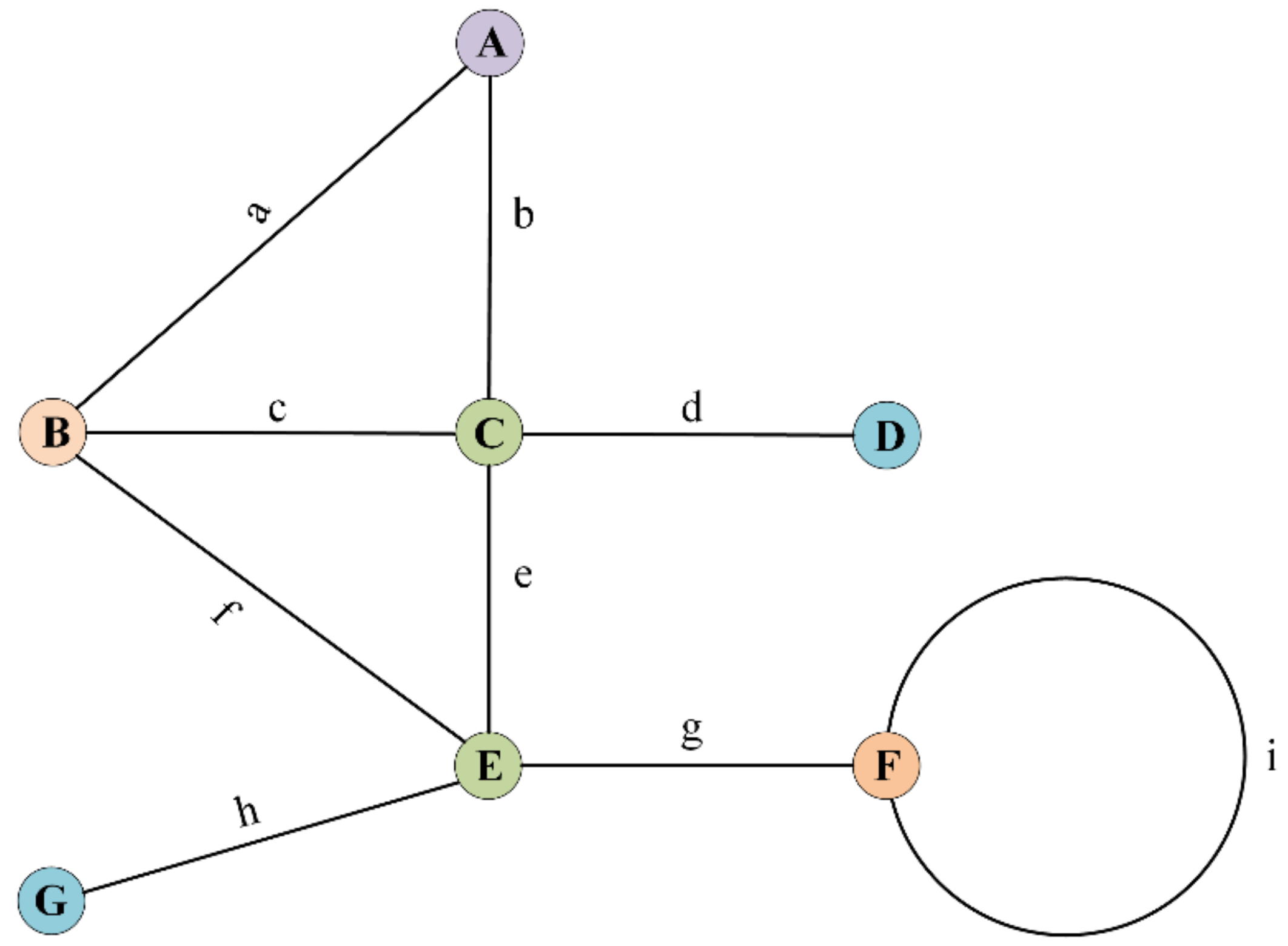
Connectedness indicates the degree of interconnection between basic units. In street networks, nodes are connected by streets, and streets intersect with streets to form new nodes (i.e., intersections). Figure 1 shows the basic network metrics. In this case, A, B, C, D, E, F, and G are nodes, where A, B, C, E, and F are intersection nodes, while D and G are dead ends. Moreover, a, b, c, d, e, f, g, h, and i are edges, and i is a self-looping edge. Given that two edges pass through it, node A is a two-way intersection. Similarly, nodes B and F are three-way intersections, and nodes C and E are four-way intersections. The proportion of node types (e.g., dead ends, three-way intersections, or four-way intersections) indicates the proportion of nodes in a street network with branches 1, 2, 3, 4, …, and n. The self-loop proportion refers to the proportion of edges with a single incident node. The metric “average streets per node” indicates the average number of edges passing through a node. It is frequently used to measure connectedness. In our study, the “average streets per node” in an undirected graph was selected as the metric for measuring the connectedness of a street network.
3.2.2. Circuity
Circuity refers to the degree of tortuous path. It is commonly used to measure the additional cost of travel to urban residents due to distance factors. In our study, 50,000 pairs of nodes with starting and ending points were simulated as random routes for each city and network type.
The circuity of each route was calculated by using Equation (2).
where represents circuity, represents the distance of the shortest path between the starting and ending points of a route, and represents the great circle distance between these nodes. Therefore, is the ratio of the network distance of the shortest path from the start to the end of each route to the great circle distance. Average circuity was selected as a metric for measuring the tortuous degree of a street network in our study.
3.2.3. Street Network Orientation Entropy
Information entropy has been used in street network research: the orientation property of a street is considered the target, and street network orientation entropy is used to measure the nature of spatial order/disorder in the orientations of street networks [29].
The simplified street network orientation entropy (without considering length weighting) was calculated by using Equation (3).
where represents the number of bins, and each bin represents a certain range around the orientation of a street. represents the index value of a bin, represents the frequency of a street falling into the th bin, and represents the proportion (probability) of a street falling into the th bin. Street network orientation entropy , which is measured in a dimensionless unit called “nats” or the natural unit of an information bit (1 nat ≈ 1.44 bits).
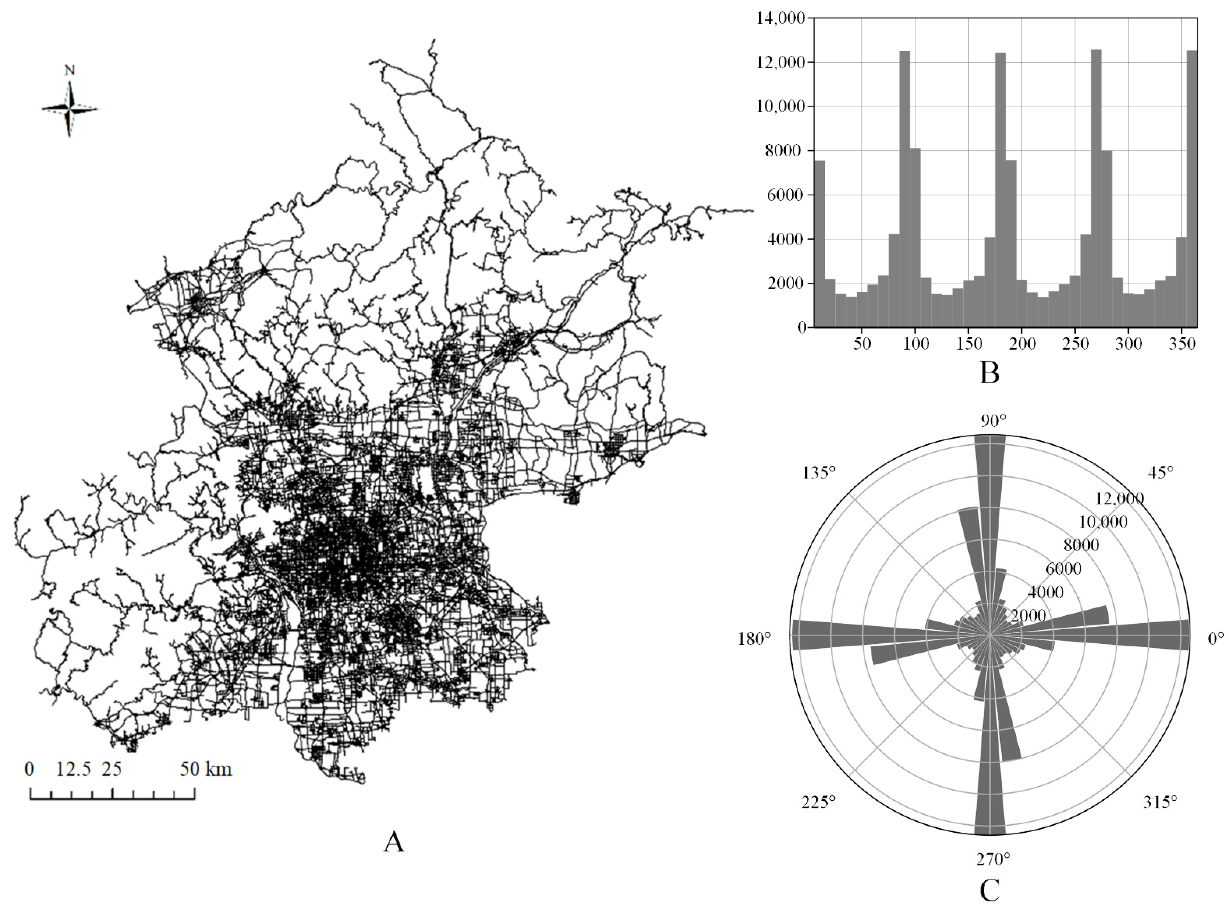
A total of 36 bins with the same size were divided for street frequency statistics, with each bin having a range of 10°. Each bin was shifted by −5° to ensure that the values are distributed in the center of the bin [29]. The orientation angles of each street segment were calculated and counted in the corresponding bin. The histogram and rose illustration were obtained, using OSMnx, on the basis of the frequency of street segments in the bin. The entropy of the street orientations was calculated by using Equation (3). For example, a street network in Beijing (Figure 2A) was used to calculate the street orientation histogram and rose illustration, as shown in Figure 2B,C, respectively. From Equation (3), the highest value of the street network orientation entropy is equal to the logarithm of the number of bins n. At this moment,; that is, the entropy of the street orientations is distributed perfectly in all the bins. If the number of bins is 36, then the highest entropy of the street orientation will be 3.584 nats. When all the street orientations are located in the same bin, the entropy of the street orientation will have the lowest value of 0. The entropy of the street orientation is 1.386 nats when all the streets are distributed in equal proportions in the bins in the east–south–west–north directions of the rose illustration.
4. Results
4.1. Spatial Distribution Characteristics of RDLS
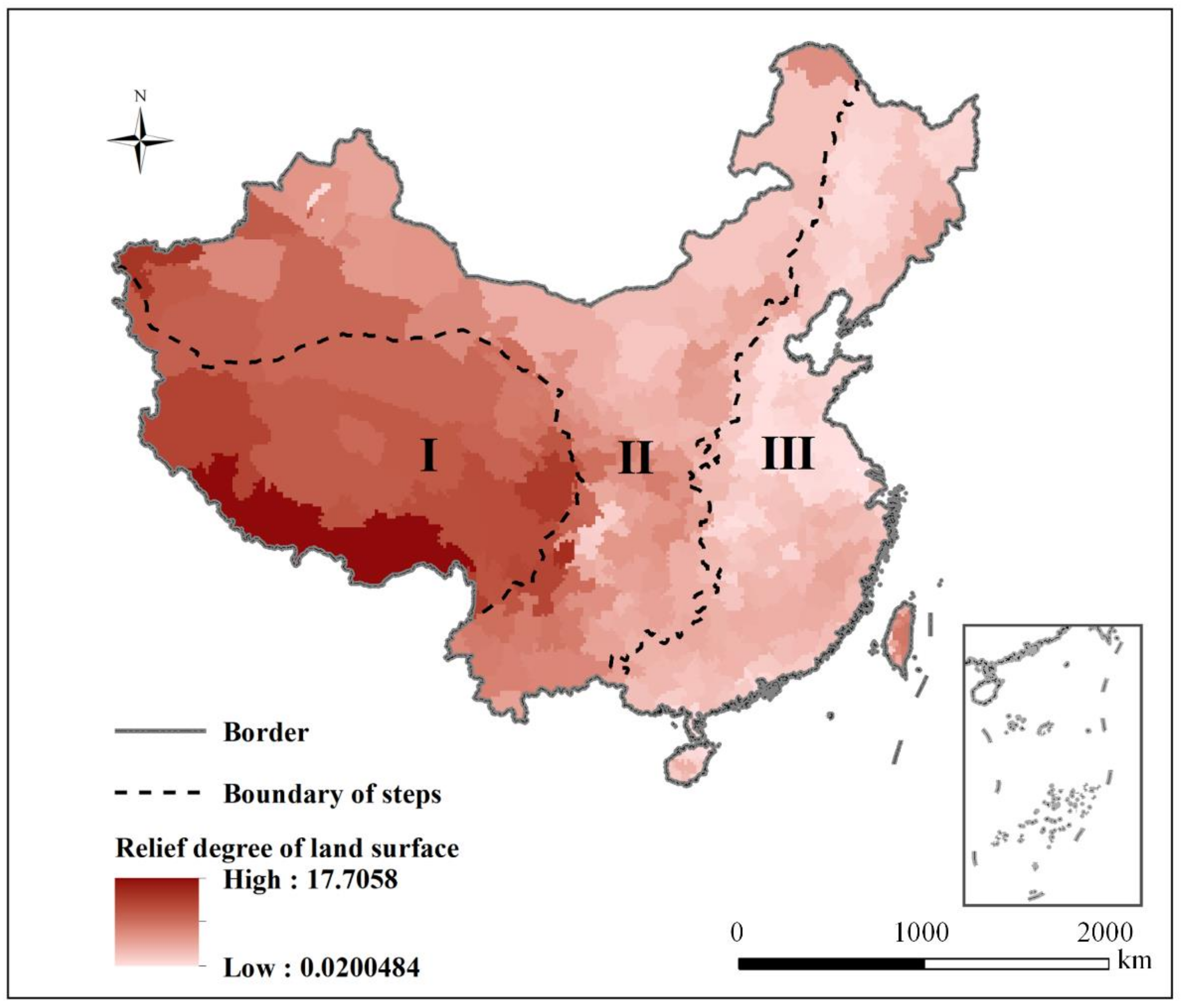
Equation (1) was used to calculate RDLS at the municipal levels, which ranged from 0 to 17.7. The result presented evident regional differences and a clear stair-stepping characteristic in the east–west direction. Such finding is basically consistent with the three steps of China’s terrain (Figure 3).
4.2. Graduation Statistics of RDLS
In our study, the basic network metrics were calculated by using the aforementioned method. The metrics included grain (), average circuity () and connectedness (the average streets per node (), proportion of dead ends (), proportion of three-way intersections (), and proportion of four-way intersections ()). The street orientation histogram and rose illustration were generated by calculating the angle of street orientation. The street network orientation entropy () for each municipal street network in the country was calculated by using Equation (3). Finally, ALT and RDLS were obtained by using Equation (1). Table 1 provides the partial results of each metric for prefecture-level cities in China. The details of the results for all the cities can be found in the Appendix A.
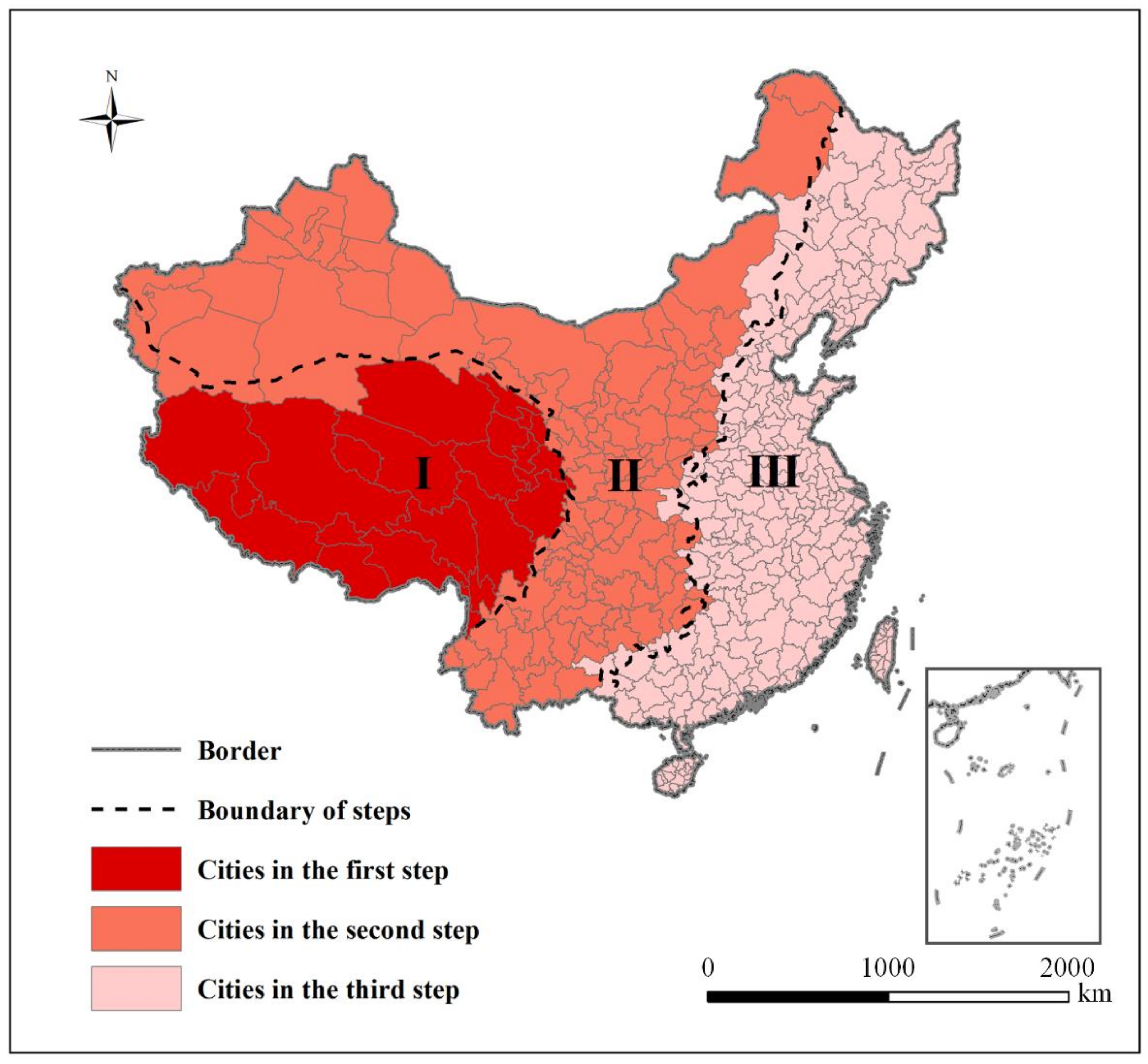
China, in topography, forms a three-step “staircase” according to altitude. As shown in Figure 4, the dotted lines are the dividing lines of the three steps on the surface. All cities are divided into three categories based on the dotted lines. The street network of cities with a high street density is frequently located in the city’s administrative center [37]. Therefore, some cities that cross the dotted line are classified according to the location of their administrative center. The classification results are presented in Figure 4, with 20 cities in the first step, 127 cities in the second step, and 244 cities in the third step.
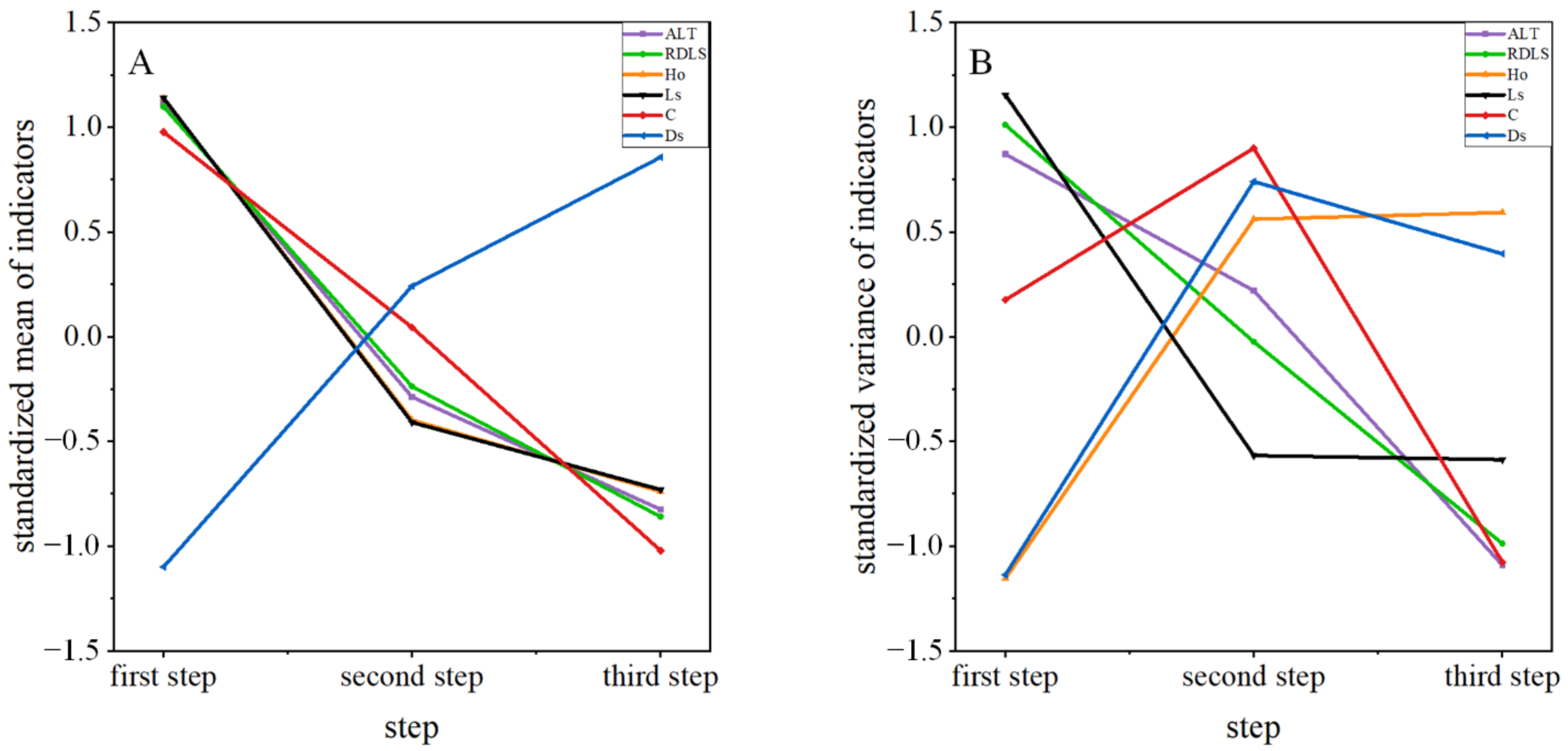
Table 2 shows the mean, maximum, minimum, and variance of street complexity-related metrics that correspond to the three steps. The mean and variance of topography, orientation entropy, grain, average circuity, and connectedness metrics were standardized by using the Z-score method. The performance of each metric in different steps was compared, as shown in Figure 5.
As shown in Figure 5, on average, the city street network in the first step exhibits the greatest RDLS, street orientation entropy, grain, and average circuity, but the lowest node connectivity. The city street network in the third step presents the smallest RDLS, street orientation entropy, grain, and path average circuity, but the highest node connectivity. For all the metrics, street network complexity exhibits the following order: first step > second step > third step. A clear correlation is also observed between street network complexity and RDLS. When evaluated in terms of grain, connectedness, circuity, and orientation entropy, the more topographic relief in a region, the higher its street network complexity.
With regard to variance, the average elevation, RDLS, and average street length of the city street network in the first step exhibit the largest dispersion, followed by that in the second step and then that in the third step. Street network orientation entropy presents the opposite degree of dispersion in the three major orders of cities, with the first step being the smallest, followed by the second step, and the third step being the largest. The urban street network in the second step has the largest dispersion in terms of circuity and average streets per node. The dispersion degree of circuity in the second step achieves the highest value, followed by that in the first step and then that in the third step. The dispersion degree of average streets per node in the three steps is ordered as follows: second step > third step > first step.
4.3. Correlation Analysis of RDLS and Street Network Complexity
Correlation analysis is a statistical analysis method for investigating the degree of correlation between two random variables in equal positions. The closeness of the relationship between two random variables (i.e., correlation) is frequently expressed by the correlation factor r. In our study, the Pearson correlation coefficient was selected for correlating RDLS with street network complexity. This coefficient is calculated by using Equation (4) [38].
where and ( = 1, 2, 3, …, n) represent the sample values of the random variables and , respectively; and and represent the sample means of the random variables and , respectively.
The correlation factor has values between −1 and 1. A correlation factor of 1 indicates that the two random variables are completely linearly and positively correlated. A correlation factor of −1 indicates that the two variables are completely negatively correlated. A correlation factor of 0 indicates that the two variables are completely uncorrelated. The closer the correlation factor is to 1 (or −1), the stronger the correlation between two random variables (positive or negative correlation). Conversely, the closer the correlation factor is to 0, the weaker the correlation between two random variables.
The total proportion of intersections with two-ways and more ways that four-ways was less than 1%, and, thus, was not considered in this study. Only the proportions of dead ends, three-way intersections, and four-way intersections were selected for analysis and research. The correlation factor between street network complexity-related metrics and RDLS was calculated separately, using Equation (4). To verify the authenticity of the linear relationship between variables, we also conducted hypothesis testing on the correlation factor by using SPSS software, as shown in Table 3.
As shown in Table 3, means street network orientation entropy (nat), means average street length (m), means average circuity, means average streets per node, means proportion of dead ends, means proportion of three-way intersections, means proportion of four-way intersections, and RDLS means relief degree of land surface.
From the results of the hypothesis testing, we see that a majority of the variables are linearly correlated with one another and significantly correlated at the 0.01 level. Only and RDLS are not significantly correlated with . As indicated in Table 3, the following conclusions can be drawn for RDLS.
- (1)
- RDLS exhibits the strongest correlation with street network circuity, with a correlation coefficient of 0.612. This result illustrates that, when RDLS is greater, the urban street network is more circuitous, and the additional travel costs for urban citizens are higher.
- (2)
- The correlation between RDLS and average street length is 0.493, indicating that, the flatter the topography, the shorter the average street network length. The average street length is largely determined by the proportions of dead ends, three-way intersections, and four-way intersections. The correlation between RDLS and dead-end proportion is 0.444, demonstrating that more dead-end nodes exist in places with greater topographic relief. This finding is probably caused by topographic relief affecting the extension and construction of roads and leading to dead-end nodes. Three-way intersection proportion exhibits an insignificant correlation with RDLS. By contrast, four-way-intersection proportion demonstrates a larger and negative correlation with RDLS (−0.499). Increasing one branch from three-way intersection to four-way intersection enhances the effect of topography; that is, regions with large RDLS are unsuitable for the construction of four-way intersections.
- (3)
- The correlation between RDLS and street network orientation entropy is 0.331, exhibiting a certain correlation. That is, when RDLS is greater, the street network is more predisposed to being distributed in different directions.
5. Discussion
A quantitative approach was used in this study to capture the pattern of street networks for a whole country. Specifically, the relationship between street network and topographic relief was analyzed quantitatively. The street network is considered to be the skeleton of the country and can reflect the physical structure [39]. We used OSMnx to extract street data of different cities from OpenStreetMap. In fact, the accuracy of OpenStreetMap data is different in different cities. Larger cities usually have higher accuracy than smaller, lesser-known cities. We recommend that the accuracy of the street network data be consistent for each city in future studies.
In addition, RDLS is an important element in the description of landforms at the macroscopic scale [36]. We used a DEM with a resolution of 30 m in calculating RDLS. We believe that, the higher the DEM resolution, the more accurate the RDLS calculation results will be. The high-resolution DEM data are expected to improve the research results. Topography was shaped by the movement of the earth’s crust, and, as described in existing studies, complex topography (such as mountains or basins) can impose constraints on the orientation of streets and their associated networks [40,41]. Topography has a strong influence on the evolving direction of the urban street network [42], while fast-growing cities lead to problems, such as efficacy of land use [43] and sustainable development [44]. Analyzing the relationship between the street network and RDLS specifically may facilitate a better understanding of the layout and development of street network patterns and their associated urban forms in China. On this basis, urban designers can plan the street layout according to the local topographic features in the fast-growing cities, not only in China, but also South America and Asia.
Previous studies on urban street networks are mostly limited to small-scale areas because of the lack of tools for obtaining standardized data sources (i.e., inconvenience of data acquisition), and thus, they cannot reflect the overall characteristics of street networks at large scales. On the basis of the spatial distribution characteristics of topographic relief at the municipal level in China, we used OSMnx-based metrics of street network complexity (i.e., grain, connectedness, circuity, and street network orientation entropy) to calculate complexity metrics for each prefecture-level city. The type of road (one-way road, two-way road, etc.), the class of street (major street, minor street, etc.), etc., were not covered; thus, they can be added to relevant studies in the future.
6. Conclusions
The contributions of this study can be reflected in three aspects:
- (1)
- On the basis of the spatial distribution characteristics of topographic relief at the municipal level in China, we determined that the spatial distribution of topographic relief was non-uniform, and the east–west direction exhibited a pattern of “high in the west and low in the east”. This finding is generally consistent with the three steps of China’s terrain. It is also similar to the results obtained by Feng et al. [36,45].
- (2)
- The dividing lines of the three terrain steps were used as the boundary for classifying the metrics of municipal street networks in China. The street network complexity presented the following order: first step > second step > third step. This result indicated that, the more undulating the topography, the higher the complexity of a street network.
- (3)
- RDLS was significantly correlated with street network complexity metrics, including street network orientation entropy, average street length, average circuity, average streets per node, dead-end proportion, and four-way intersection proportion. Among these metrics, RDLS was positively correlated with street network orientation entropy, average street length, average circuity, and the dead-end proportion. Meanwhile, it was negatively correlated with average streets per node and the four-way intersection proportion.
This study extended the research on the correlation between topographic relief and street network to a certain extent, while complementing the research methods and results on the complexity of urban street networks in China. A higher-resolution DEM and higher-accuracy street network data will help improve the research results in future studies.
Author Contributions
Study design, data analysis, and writing—original draft preparation, Nai Yang and Yi Chao; data analysis, writing result analysis, and writing—review and editing, Le Jiang and Yang Li; providing useful suggestion on data and result analysis, writing—review and editing, and supervision, Pengcheng Liu. All authors have read and agreed to the published version of the manuscript.
Funding
This research was funded by the National Natural Science Foundation of China (No. 42171438, 42071455).
Institutional Review Board Statement
Not applicable.
Informed Consent Statement
Not applicable.
Conflicts of Interest
The authors declare that they have no known competing financial interests or personal relationships that could have appeared to influence the work reported in this paper.
Appendix A

Table A1.
Calculation results of each index for prefecture-level cities.
| Beijing | 3.26 | 329 | 1.09 | 2.97 | 0.14 | 0.61 | 0.23 | 355 | 3.4 |
| Tianjin | 3.49 | 371 | 1.05 | 3 | 0.16 | 0.52 | 0.31 | 19 | 0.25 |
| Shijiazhuang | 2.75 | 328 | 1.06 | 2.93 | 0.17 | 0.56 | 0.27 | 270 | 2.56 |
| Cangzhou | 3.1 | 320 | 1.04 | 2.87 | 0.16 | 0.64 | 0.2 | 10 | 0.1 |
| Hengshui | 2.98 | 370 | 1.04 | 2.86 | 0.16 | 0.67 | 0.17 | 22 | 0.16 |
| Handan | 2.86 | 396 | 1.04 | 2.88 | 0.16 | 0.65 | 0.19 | 239 | 1.73 |
| Xingtai | 2.82 | 367 | 1.05 | 2.93 | 0.15 | 0.61 | 0.23 | 168 | 1.47 |
| Baoding | 3.02 | 543 | 1.07 | 2.92 | 0.15 | 0.61 | 0.23 | 341 | 2.59 |
| Zhangjiakou | 3.46 | 767 | 1.11 | 2.74 | 0.21 | 0.62 | 0.16 | 1254 | 4.34 |
| Chengde | 3.57 | 1027 | 1.15 | 2.5 | 0.28 | 0.64 | 0.07 | 936 | 4.72 |
| Tangshan | 3.31 | 636 | 1.06 | 2.8 | 0.21 | 0.56 | 0.22 | 57 | 0.46 |
| Qinhuangdao | 3.47 | 627 | 1.1 | 2.85 | 0.18 | 0.6 | 0.21 | 214 | 2.03 |
| Langfang | 3.12 | 459 | 1.04 | 2.9 | 0.19 | 0.54 | 0.27 | 11 | 0.41 |
| Shenyang | 3.52 | 576 | 1.06 | 3.1 | 0.11 | 0.58 | 0.29 | 56 | 0.54 |
| Huludao | 3.55 | 908 | 1.12 | 2.94 | 0.16 | 0.58 | 0.25 | 235 | 1.82 |
| Chaoyang | 3.56 | 1839 | 1.11 | 2.92 | 0.16 | 0.60 | 0.23 | 462 | 2.09 |
| Fuxin | 3.52 | 1418 | 1.10 | 2.91 | 0.15 | 0.63 | 0.21 | 200 | 0.98 |
| Jinzhou | 3.36 | 1195 | 1.09 | 2.98 | 0.14 | 0.58 | 0.26 | 81 | 0.87 |
| Panjin | 3.41 | 983 | 1.06 | 3.16 | 0.12 | 0.48 | 0.38 | 9 | 0.02 |
| Fushun | 3.46 | 1117 | 1.15 | 2.86 | 0.16 | 0.66 | 0.17 | 409 | 2.85 |
| Yingkou | 3.42 | 879 | 1.08 | 3.03 | 0.15 | 0.51 | 0.33 | 167 | 1.33 |
| Dalian | 3.55 | 602 | 1.11 | 2.95 | 0.14 | 0.64 | 0.21 | 79 | 0.97 |
| Dandong | 3.56 | 1353 | 1.19 | 2.78 | 0.20 | 0.63 | 0.17 | 255 | 2.14 |
| Benxi | 3.56 | 1063 | 1.23 | 2.97 | 0.13 | 0.64 | 0.22 | 469 | 2.72 |
| Liaoyang | 3.48 | 892 | 1.10 | 2.87 | 0.19 | 0.57 | 0.24 | 154 | 1.44 |
| Anshan | 3.46 | 1043 | 1.11 | 2.97 | 0.16 | 0.56 | 0.28 | 166 | 1.30 |
| Tieling | 3.55 | 984 | 1.10 | 2.73 | 0.22 | 0.60 | 0.17 | 182 | 1.17 |
| Changchun | 3.49 | 465 | 1.06 | 2.99 | 0.15 | 0.56 | 0.28 | 197 | 0.75 |
| Jilin | 3.49 | 322 | 1.09 | 2.46 | 0.33 | 0.55 | 0.12 | 383 | 2.12 |
| Baishan | 3.56 | 1369 | 1.27 | 2.68 | 0.24 | 0.59 | 0.16 | 831 | 4.21 |
| Yanbian | 3.53 | 621 | 1.16 | 2.74 | 0.23 | 0.58 | 0.19 | 658 | 4.56 |
| Tonghua | 3.56 | 1106 | 1.15 | 2.69 | 0.23 | 0.60 | 0.16 | 527 | 2.84 |
| Liaoyuan | 3.55 | 1140 | 1.10 | 2.79 | 0.20 | 0.61 | 0.18 | 364 | 1.20 |
| Siping | 3.48 | 679 | 1.06 | 2.61 | 0.27 | 0.56 | 0.16 | 192 | 0.72 |
| Songyuan | 3.47 | 1104 | 1.06 | 2.82 | 0.18 | 0.65 | 0.17 | 153 | 0.38 |
| Baicheng | 3.37 | 698 | 1.06 | 2.74 | 0.22 | 0.61 | 0.17 | 155 | 0.54 |
| Harbin | 3.50 | 607 | 1.10 | 2.84 | 0.20 | 0.56 | 0.23 | 241 | 2.05 |
| Mudanjiang | 3.53 | 454 | 1.15 | 2.75 | 0.24 | 0.55 | 0.22 | 528 | 2.75 |
| Jixi | 3.54 | 382 | 1.10 | 2.68 | 0.25 | 0.58 | 0.17 | 166 | 0.97 |
| Qitaihe | 3.51 | 496 | 1.08 | 3.02 | 0.13 | 0.60 | 0.25 | 270 | 1.17 |
| Shuangyashan | 3.38 | 648 | 1.09 | 2.84 | 0.20 | 0.57 | 0.23 | 149 | 1.02 |
| Jiamusi | 3.14 | 349 | 1.08 | 2.80 | 0.20 | 0.60 | 0.20 | 95 | 0.73 |
| Suihua | 3.36 | 863 | 1.07 | 2.76 | 0.21 | 0.61 | 0.18 | 196 | 0.78 |
| Yichun | 3.53 | 930 | 1.13 | 2.73 | 0.24 | 0.55 | 0.21 | 404 | 2.15 |
| Hegang | 3.35 | 912 | 1.08 | 2.88 | 0.18 | 0.57 | 0.25 | 200 | 1.24 |
| Daqing | 3.48 | 859 | 1.06 | 2.99 | 0.14 | 0.58 | 0.27 | 132 | 0.25 |
| Qiqihar | 3.42 | 781 | 1.07 | 2.83 | 0.20 | 0.58 | 0.22 | 198 | 0.65 |
| Daxinganling | 3.32 | 1420 | 1.18 | 2.87 | 0.20 | 0.53 | 0.27 | 571 | 6.20 |
| Heihe | 3.39 | 764 | 1.11 | 2.80 | 0.22 | 0.55 | 0.23 | 364 | 0.96 |
| Huhhot | 3.30 | 577 | 1.08 | 2.82 | 0.20 | 0.59 | 0.21 | 1369 | 3.11 |
| Baotou | 3.31 | 418 | 1.06 | 2.78 | 0.21 | 0.60 | 0.19 | 1396 | 2.68 |
| Bayannur | 3.40 | 906 | 1.07 | 2.75 | 0.21 | 0.63 | 0.16 | 1275 | 2.57 |
| Eerduosi | 3.53 | 887 | 1.06 | 3.12 | 0.13 | 0.48 | 0.38 | 1296 | 1.94 |
| Wuhai | 3.18 | 591 | 1.07 | 3.06 | 0.13 | 0.51 | 0.34 | 1319 | 2.82 |
| Alxa | 3.09 | 1190 | 1.07 | 2.74 | 0.21 | 0.62 | 0.17 | 1263 | 3.83 |
| Ulanqab | 3.43 | 676 | 1.08 | 2.79 | 0.19 | 0.63 | 0.18 | 1406 | 2.87 |
| Xilingol | 3.44 | 1704 | 1.09 | 2.79 | 0.22 | 0.55 | 0.23 | 1104 | 1.96 |
| Chifeng | 3.51 | 665 | 1.10 | 2.79 | 0.20 | 0.64 | 0.16 | 868 | 2.75 |
| Tongliao | 3.23 | 604 | 1.07 | 2.84 | 0.19 | 0.58 | 0.22 | 334 | 1.25 |
| Hinggan | 3.51 | 1030 | 1.09 | 2.76 | 0.23 | 0.54 | 0.22 | 589 | 2.59 |
| Hulunbuir | 3.49 | 1130 | 1.12 | 2.79 | 0.21 | 0.58 | 0.21 | 697 | 2.34 |
| Taiyuan | 3.32 | 434 | 1.11 | 3.01 | 0.13 | 0.60 | 0.26 | 1262 | 4.44 |
| Lvliang | 3.46 | 813 | 1.14 | 2.67 | 0.25 | 0.60 | 0.15 | 1225 | 5.16 |
| Jinzhong | 3.44 | 666 | 1.11 | 2.75 | 0.22 | 0.61 | 0.17 | 1176 | 4.42 |
| Yangquan | 3.53 | 781 | 1.13 | 2.65 | 0.25 | 0.59 | 0.15 | 1033 | 3.75 |
| Xinzhou | 3.52 | 839 | 1.14 | 2.61 | 0.26 | 0.61 | 0.13 | 1399 | 5.42 |
| Shuozhou | 3.31 | 735 | 1.08 | 2.78 | 0.21 | 0.58 | 0.20 | 1350 | 3.16 |
| Datong | 3.37 | 721 | 1.10 | 2.76 | 0.22 | 0.58 | 0.19 | 1302 | 3.62 |
| Linfen | 3.52 | 993 | 1.17 | 2.64 | 0.25 | 0.59 | 0.15 | 992 | 4.56 |
| Changzhi | 3.45 | 619 | 1.11 | 2.75 | 0.23 | 0.55 | 0.21 | 1161 | 4.43 |
| Jincheng | 3.51 | 737 | 1.17 | 2.75 | 0.22 | 0.59 | 0.18 | 987 | 4.51 |
| Yuncheng | 3.46 | 864 | 1.12 | 2.78 | 0.22 | 0.55 | 0.22 | 609 | 3.10 |
| Zhengzhou | 3.12 | 387 | 1.05 | 3.14 | 0.12 | 0.49 | 0.38 | 236 | 1.67 |
| Kaifeng | 3.02 | 458 | 1.04 | 2.91 | 0.17 | 0.59 | 0.24 | 69 | 0.14 |
| Shangqiu | 3.13 | 984 | 1.03 | 3.00 | 0.17 | 0.48 | 0.33 | 48 | 0.19 |
| Sanmenxia | 3.51 | 1033 | 1.18 | 2.92 | 0.18 | 0.52 | 0.28 | 881 | 3.73 |
| Luoyang | 3.43 | 637 | 1.12 | 2.97 | 0.15 | 0.57 | 0.26 | 649 | 3.78 |
| Jiyuan | 2.84 | 579 | 1.11 | 3.17 | 0.12 | 0.47 | 0.40 | 415 | 2.90 |
| Jiaozuo | 3.02 | 307 | 1.04 | 2.90 | 0.19 | 0.53 | 0.28 | 180 | 1.52 |
| Xinxiang | 3.11 | 308 | 1.04 | 2.89 | 0.18 | 0.56 | 0.26 | 155 | 1.50 |
| Hebi | 2.95 | 248 | 1.05 | 2.88 | 0.20 | 0.51 | 0.28 | 154 | 1.17 |
| Anyang | 3.01 | 342 | 1.06 | 2.86 | 0.17 | 0.62 | 0.20 | 218 | 1.67 |
| Puyang | 3.00 | 387 | 1.03 | 2.93 | 0.15 | 0.61 | 0.23 | 50 | 0.13 |
| Pingdingshan | 3.30 | 639 | 1.07 | 3.01 | 0.13 | 0.61 | 0.25 | 253 | 2.71 |
| Xuchang | 3.12 | 798 | 1.05 | 3.04 | 0.16 | 0.48 | 0.35 | 129 | 1.01 |
| Luohe | 2.94 | 660 | 1.04 | 3.06 | 0.15 | 0.49 | 0.35 | 63 | 0.12 |
| Zhoukou | 3.05 | 938 | 1.04 | 2.91 | 0.19 | 0.50 | 0.29 | 47 | 0.23 |
| Zhumadian | 3.07 | 1132 | 1.05 | 2.94 | 0.17 | 0.54 | 0.28 | 93 | 0.91 |
| Xinyang | 3.38 | 935 | 1.06 | 2.81 | 0.20 | 0.57 | 0.22 | 118 | 1.53 |
| Nanyang | 3.43 | 1150 | 1.09 | 2.95 | 0.18 | 0.52 | 0.29 | 307 | 2.95 |
| Jinan | 3.28 | 449 | 1.09 | 3.04 | 0.13 | 0.56 | 0.29 | 162 | 1.19 |
| Liaocheng | 2.98 | 620 | 1.03 | 3.08 | 0.15 | 0.47 | 0.37 | 37 | 0.23 |
| Dezhou | 3.09 | 739 | 1.04 | 3.13 | 0.14 | 0.44 | 0.41 | 21 | 0.18 |
| Binzhou | 2.98 | 582 | 1.03 | 3.13 | 0.16 | 0.38 | 0.46 | 16 | 0.24 |
| Dongying | 2.96 | 719 | 1.03 | 3.20 | 0.12 | 0.43 | 0.43 | 11 | 0.21 |
| Zibo | 3.05 | 643 | 1.06 | 3.13 | 0.13 | 0.46 | 0.39 | 218 | 1.63 |
| Weifang | 2.85 | 454 | 1.04 | 3.12 | 0.15 | 0.44 | 0.41 | 108 | 0.98 |
| Yantai | 3.30 | 664 | 1.06 | 3.06 | 0.15 | 0.49 | 0.35 | 105 | 0.86 |
| Weihai | 3.35 | 501 | 1.06 | 3.05 | 0.14 | 0.51 | 0.33 | 62 | 0.84 |
| Qingdao | 3.20 | 298 | 1.04 | 2.96 | 0.18 | 0.50 | 0.31 | 53 | 0.82 |
| Rizhao | 3.24 | 636 | 1.06 | 3.13 | 0.14 | 0.46 | 0.38 | 137 | 0.84 |
| Linyi | 3.14 | 455 | 1.05 | 2.94 | 0.18 | 0.53 | 0.27 | 155 | 1.38 |
| Taian | 3.31 | 601 | 1.07 | 2.91 | 0.18 | 0.55 | 0.27 | 158 | 1.57 |
| Jining | 3.00 | 621 | 1.04 | 3.13 | 0.14 | 0.44 | 0.41 | 63 | 0.60 |
| Zaozhuang | 3.02 | 376 | 1.05 | 3.02 | 0.15 | 0.54 | 0.30 | 94 | 0.73 |
| Heze | 2.98 | 782 | 1.04 | 3.01 | 0.15 | 0.54 | 0.31 | 52 | 0.20 |
| Nanjing | 3.55 | 408 | 1.07 | 3.06 | 0.13 | 0.55 | 0.30 | 27 | 0.53 |
| Zhenjiang | 3.48 | 419 | 1.05 | 2.96 | 0.16 | 0.57 | 0.26 | 29 | 0.40 |
| Changzhou | 3.37 | 381 | 1.05 | 3.10 | 0.12 | 0.53 | 0.33 | 21 | 0.28 |
| Wuxi | 3.47 | 311 | 1.05 | 3.08 | 0.13 | 0.52 | 0.33 | 21 | 0.16 |
| Suzhou | 3.46 | 398 | 1.06 | 3.11 | 0.12 | 0.53 | 0.34 | 11 | 0.06 |
| Nantong | 3.40 | 465 | 1.04 | 3.01 | 0.17 | 0.49 | 0.33 | 9 | 0.02 |
| Taizhou | 3.41 | 385 | 1.05 | 2.74 | 0.24 | 0.53 | 0.22 | 10 | 0.02 |
| Yangzhou | 3.33 | 434 | 1.04 | 2.70 | 0.26 | 0.53 | 0.21 | 9 | 0.13 |
| Suqian | 3.21 | 707 | 1.04 | 3.01 | 0.17 | 0.47 | 0.35 | 10 | 0.15 |
| Huaian | 3.35 | 723 | 1.04 | 3.00 | 0.17 | 0.49 | 0.33 | 12 | 0.24 |
| Yancheng | 3.44 | 710 | 1.04 | 2.92 | 0.20 | 0.46 | 0.33 | 9 | 0.02 |
| Lianyungang | 3.37 | 616 | 1.05 | 3.00 | 0.18 | 0.48 | 0.33 | 20 | 0.25 |
| Xuzhou | 3.28 | 725 | 1.04 | 3.00 | 0.16 | 0.52 | 0.31 | 29 | 0.41 |
| Hefei | 3.44 | 446 | 1.06 | 3.09 | 0.14 | 0.50 | 0.35 | 37 | 0.55 |
| Huainan | 3.42 | 599 | 1.06 | 2.75 | 0.23 | 0.56 | 0.21 | 23 | 0.16 |
| Luan | 3.47 | 786 | 1.11 | 2.95 | 0.17 | 0.52 | 0.30 | 212 | 2.20 |
| Fuyang | 3.25 | 551 | 1.05 | 2.93 | 0.17 | 0.57 | 0.25 | 33 | 0.22 |
| Bozhou | 3.03 | 785 | 1.04 | 3.01 | 0.15 | 0.54 | 0.31 | 28 | 0.14 |
| Huaibei | 3.03 | 605 | 1.04 | 2.95 | 0.20 | 0.45 | 0.34 | 24 | 0.28 |
| Suzhou | 3.13 | 819 | 1.04 | 3.12 | 0.14 | 0.44 | 0.40 | 27 | 0.33 |
| Bengbu | 3.30 | 656 | 1.05 | 3.09 | 0.14 | 0.48 | 0.36 | 15 | 0.39 |
| Chuzhou | 3.44 | 808 | 1.07 | 2.93 | 0.19 | 0.49 | 0.31 | 44 | 0.71 |
| Maanshan | 3.43 | 522 | 1.09 | 2.85 | 0.19 | 0.58 | 0.22 | 22 | 0.61 |
| Wuhu | 3.46 | 627 | 1.07 | 2.99 | 0.14 | 0.57 | 0.28 | 30 | 0.76 |
| Tongling | 3.58 | 972 | 1.07 | 2.97 | 0.15 | 0.57 | 0.27 | 43 | 0.76 |
| Anqing | 3.57 | 895 | 1.13 | 2.95 | 0.17 | 0.54 | 0.28 | 216 | 2.52 |
| Chizhou | 3.52 | 1189 | 1.13 | 2.86 | 0.19 | 0.56 | 0.24 | 182 | 3.05 |
| Huangshan | 3.57 | 966 | 1.27 | 2.56 | 0.28 | 0.60 | 0.12 | 381 | 3.75 |
| Xuancheng | 3.53 | 963 | 1.12 | 2.84 | 0.20 | 0.54 | 0.25 | 206 | 2.21 |
| Shanghai | 3.49 | 339 | 1.04 | 3.02 | 0.15 | 0.52 | 0.31 | 9 | 2.21 |
| Hangzhou | 3.52 | 419 | 1.14 | 2.90 | 0.18 | 0.55 | 0.26 | 286 | 3.04 |
| Huzhou | 3.46 | 600 | 1.09 | 2.98 | 0.17 | 0.52 | 0.31 | 120 | 1.53 |
| Jiaxing | 3.36 | 508 | 1.05 | 3.07 | 0.15 | 0.48 | 0.36 | 9 | 0.03 |
| Shaoxing | 3.53 | 555 | 1.12 | 2.89 | 0.19 | 0.54 | 0.26 | 187 | 2.52 |
| Ningbo | 3.54 | 395 | 1.10 | 3.03 | 0.15 | 0.51 | 0.33 | 146 | 1.32 |
| Zhoushan | 3.56 | 418 | 1.10 | 3.00 | 0.15 | 0.55 | 0.29 | 57 | 0.59 |
| Taizhou | 3.54 | 565 | 1.13 | 2.93 | 0.17 | 0.56 | 0.27 | 257 | 2.32 |
| Quzhou | 3.57 | 513 | 1.15 | 2.69 | 0.25 | 0.56 | 0.18 | 338 | 2.69 |
| Jinhua | 3.54 | 403 | 1.11 | 2.96 | 0.17 | 0.54 | 0.28 | 300 | 2.66 |
| Lishui | 3.58 | 1005 | 1.37 | 2.68 | 0.24 | 0.59 | 0.16 | 628 | 4.22 |
| Wenzhou | 3.58 | 479 | 1.16 | 2.91 | 0.19 | 0.53 | 0.27 | 368 | 2.96 |
| Nanchang | 3.51 | 457 | 1.09 | 2.97 | 0.14 | 0.60 | 0.24 | 34 | 0.72 |
| Jiujiang | 3.53 | 831 | 1.10 | 2.89 | 0.17 | 0.58 | 0.23 | 215 | 2.80 |
| Jingdezhen | 3.57 | 680 | 1.13 | 2.49 | 0.31 | 0.58 | 0.10 | 142 | 2.92 |
| Shangrao | 3.58 | 665 | 1.17 | 2.47 | 0.32 | 0.57 | 0.11 | 206 | 3.45 |
| Yingtan | 3.49 | 497 | 1.10 | 2.77 | 0.22 | 0.57 | 0.20 | 165 | 2.58 |
| Fuzhou | 3.57 | 1070 | 1.12 | 2.78 | 0.21 | 0.60 | 0.18 | 226 | 2.97 |
| Xinyu | 3.36 | 1074 | 1.10 | 2.95 | 0.17 | 0.53 | 0.29 | 122 | 1.41 |
| Yichun | 3.56 | 1146 | 1.14 | 2.88 | 0.18 | 0.57 | 0.24 | 222 | 2.70 |
| Pingxiang | 3.57 | 990 | 1.14 | 2.88 | 0.17 | 0.61 | 0.21 | 332 | 3.33 |
| Jian | 3.54 | 1134 | 1.14 | 2.80 | 0.21 | 0.57 | 0.22 | 251 | 3.28 |
| Ganzhou | 3.55 | 631 | 1.15 | 2.81 | 0.20 | 0.58 | 0.21 | 365 | 3.72 |
| Fuzhou | 3.56 | 483 | 1.19 | 2.93 | 0.15 | 0.61 | 0.23 | 365 | 2.74 |
| Ningde | 3.56 | 1067 | 1.38 | 2.74 | 0.21 | 0.62 | 0.16 | 575 | 3.47 |
| Sanming | 3.58 | 1106 | 1.25 | 2.73 | 0.19 | 0.68 | 0.12 | 557 | 3.99 |
| Putian | 3.57 | 744 | 1.16 | 2.89 | 0.18 | 0.58 | 0.24 | 348 | 2.87 |
| Nanping | 3.45 | 722 | 1.24 | 2.36 | 0.09 | 0.32 | 0.06 | 500 | 4.50 |
| Quanzhou | 3.56 | 380 | 1.14 | 2.56 | 0.11 | 0.37 | 0.14 | 443 | 3.37 |
| Xiamen | 3.55 | 271 | 1.09 | 3.04 | 0.11 | 0.63 | 0.25 | 195 | 1.70 |
| Zhangzhou | 3.57 | 419 | 1.13 | 2.77 | 0.19 | 0.65 | 0.16 | 306 | 2.67 |
| Longyan | 3.57 | 1084 | 1.25 | 2.76 | 0.19 | 0.67 | 0.13 | 584 | 3.88 |
| Taipei | 3.45 | 127 | 1.08 | 3.11 | 0.11 | 0.56 | 0.31 | 78 | 1.16 |
| New Taipei | 3.58 | 224 | 1.20 | 2.84 | 0.19 | 0.59 | 0.21 | 384 | 4.00 |
| Taoyuan | 3.57 | 187 | 1.09 | 2.84 | 0.20 | 0.57 | 0.22 | 400 | 3.03 |
| Taichung | 3.51 | 163 | 1.10 | 2.93 | 0.18 | 0.55 | 0.27 | 1004 | 6.80 |
| Tainan | 3.49 | 323 | 1.09 | 3.26 | 0.07 | 0.53 | 0.38 | 80 | 1.14 |
| Kaohsiung | 3.54 | 146 | 1.08 | 3.07 | 0.12 | 0.56 | 0.30 | 776 | 6.71 |
| Keelung | 3.55 | 149 | 1.14 | 2.84 | 0.19 | 0.57 | 0.21 | 126 | 1.32 |
| Hsinchu | 3.53 | 200 | 1.16 | 2.81 | 0.21 | 0.57 | 0.21 | 792 | 7.40 |
| Chiayi | 3.50 | 310 | 1.18 | 2.84 | 0.18 | 0.62 | 0.19 | 537 | 4.57 |
| Miaoli County | 3.55 | 308 | 1.16 | 2.96 | 0.15 | 0.59 | 0.24 | 676 | 5.78 |
| Changhua County | 3.51 | 244 | 1.05 | 2.94 | 0.17 | 0.57 | 0.25 | 35 | 0.29 |
| Yunlin County | 3.50 | 290 | 1.06 | 2.94 | 0.16 | 0.60 | 0.24 | 72 | 1.05 |
| Nantou County | 3.56 | 341 | 1.30 | 2.81 | 0.19 | 0.61 | 0.19 | 1250 | 8.19 |
| Yilan County | 3.55 | 206 | 1.08 | 2.94 | 0.16 | 0.59 | 0.24 | 919 | 7.33 |
| Taitung County | 3.57 | 255 | 1.19 | 2.81 | 0.21 | 0.58 | 0.21 | 1070 | 7.73 |
| Hualien County | 3.43 | 223 | 1.12 | 2.95 | 0.16 | 0.56 | 0.27 | 1389 | 8.39 |
| Pingtung County | 3.52 | 236 | 1.08 | 2.85 | 0.18 | 0.60 | 0.21 | 387 | 3.92 |
| Kinmen County | 3.48 | 218 | 1.07 | 2.77 | 0.19 | 0.65 | 0.15 | 21 | 0.13 |
| Lianjiang County | 3.49 | ||||||||
| Penghu County | 3.49 | ||||||||
| Guangzhou | 3.54 | 264 | 1.09 | 2.93 | 0.14 | 0.66 | 0.19 | 113 | 1.55 |
| Dongguan | 3.58 | 291 | 1.06 | 2.99 | 0.14 | 0.60 | 0.25 | 42 | 0.65 |
| Shenzhen | 3.53 | 209 | 1.08 | 3.00 | 0.12 | 0.64 | 0.23 | 79 | 1.13 |
| Huizhou | 3.56 | 579 | 1.13 | 2.79 | 0.19 | 0.62 | 0.17 | 165 | 1.87 |
| Shanwei | 3.56 | 548 | 1.10 | 2.71 | 0.23 | 0.59 | 0.17 | 145 | 1.61 |
| Shantou | 3.57 | 378 | 1.08 | 2.85 | 0.18 | 0.60 | 0.21 | 49 | 0.48 |
| Jieyang | 3.54 | 626 | 1.09 | 2.82 | 0.21 | 0.56 | 0.23 | 157 | 1.64 |
| Chaozhou | 3.58 | 340 | 1.12 | 2.70 | 0.22 | 0.64 | 0.14 | 220 | 2.33 |
| Meizhou | 3.58 | 1074 | 1.19 | 2.80 | 0.18 | 0.67 | 0.15 | 299 | 3.01 |
| Heyuan | 3.57 | 1167 | 1.21 | 2.71 | 0.21 | 0.65 | 0.13 | 294 | 2.72 |
| Shaoguan | 3.58 | 1076 | 1.21 | 2.73 | 0.20 | 0.66 | 0.13 | 416 | 3.69 |
| Qingyuan | 3.55 | 575 | 1.16 | 2.85 | 0.19 | 0.60 | 0.21 | 348 | 3.30 |
| Foshan | 3.52 | 240 | 1.07 | 2.92 | 0.14 | 0.66 | 0.19 | 31 | 0.58 |
| Zhaoqing | 3.57 | 652 | 1.16 | 2.81 | 0.19 | 0.61 | 0.19 | 223 | 3.20 |
| Zhongshan | 3.55 | 216 | 1.07 | 2.91 | 0.14 | 0.66 | 0.19 | 27 | 0.40 |
| Zhuhai | 3.52 | 273 | 1.09 | 3.01 | 0.11 | 0.65 | 0.23 | 38 | 0.54 |
| Jiangmen | 3.57 | 364 | 1.11 | 2.86 | 0.16 | 0.64 | 0.18 | 89 | 1.56 |
| Yunfu | 3.57 | 635 | 1.17 | 2.91 | 0.16 | 0.62 | 0.22 | 215 | 2.52 |
| Yangjiang | 3.54 | 544 | 1.10 | 2.91 | 0.17 | 0.58 | 0.25 | 157 | 2.06 |
| Maoming | 3.53 | 707 | 1.13 | 2.79 | 0.17 | 0.69 | 0.13 | 194 | 2.66 |
| Zhenjiang | 3.55 | 682 | 1.11 | 2.90 | 0.15 | 0.67 | 0.18 | 37 | 0.37 |
| Haikou | 3.54 | 361 | 1.09 | 2.82 | 0.19 | 0.61 | 0.19 | 46 | 0.18 |
| Wenchang | 3.54 | 677 | 1.11 | 2.50 | 0.32 | 0.54 | 0.14 | 33 | 0.33 |
| Qionghai | 3.55 | 738 | 1.15 | 2.74 | 0.21 | 0.64 | 0.14 | 84 | 1.50 |
| Wanning | 3.52 | 712 | 1.11 | 2.82 | 0.19 | 0.61 | 0.19 | 112 | 1.19 |
| Lingshui County | 3.56 | 456 | 1.12 | 2.75 | 0.21 | 0.59 | 0.18 | 69 | 0.78 |
| Sanya | 3.55 | 369 | 1.12 | 2.81 | 0.19 | 0.63 | 0.17 | 154 | 1.41 |
| Dongfang City | 3.50 | 877 | 1.14 | 2.62 | 0.26 | 0.58 | 0.15 | 202 | 1.83 |
| Changjiang County | 3.48 | 743 | 1.13 | 2.83 | 0.17 | 0.66 | 0.17 | 276 | 2.57 |
| Ledong County | 3.56 | 850 | 1.13 | 2.60 | 0.28 | 0.56 | 0.16 | 211 | 1.70 |
| Danzhou | 3.55 | 673 | 1.10 | 2.67 | 0.26 | 0.56 | 0.18 | 113 | 1.27 |
| Lingao County | 3.56 | 884 | 1.08 | 2.59 | 0.28 | 0.56 | 0.15 | 77 | 0.41 |
| Chengmai County | 3.55 | 645 | 1.13 | 2.63 | 0.25 | 0.60 | 0.14 | 86 | 0.64 |
| Tunchang County | 3.50 | 608 | 1.16 | 2.68 | 0.23 | 0.61 | 0.15 | 183 | 1.20 |
| Baisha County | 3.51 | 1292 | 1.32 | 2.51 | 0.31 | 0.58 | 0.11 | 492 | 3.67 |
| Qiongzhong County | 3.56 | 1156 | 1.27 | 2.40 | 0.33 | 0.61 | 0.06 | 442 | 3.54 |
| Dingan County | 3.56 | 789 | 1.14 | 2.59 | 0.25 | 0.63 | 0.63 | 95 | 0.53 |
| Baoting County | 3.54 | 1034 | 1.22 | 2.47 | 0.3 | 0.63 | 0.07 | 316 | 2.46 |
| Wuzhishan | 3.56 | 1357 | 1.33 | 2.47 | 0.3 | 0.64 | 0.06 | 619 | 3.7 |
| Sansha | 2.53 | 255 | 1.04 | 3.02 | 0.05 | 0.83 | 0.12 | 0 | 0.00 |
| Hong Kong | 3.58 | 157 | 1.13 | 2.86 | 0.14 | 0.68 | 0.16 | 121 | 1.37 |
| Macau | 3.55 | 93 | 1.09 | 3.01 | 0.08 | 0.73 | 0.17 | 10 | 0.07 |
| Nanning | 3.54 | 818 | 1.10 | 2.88 | 0.18 | 0.57 | 0.24 | 195 | 3.04 |
| Laibin | 3.54 | 1145 | 1.16 | 2.65 | 0.23 | 0.64 | 0.12 | 282 | 3.05 |
| Guigang | 3.54 | 1031 | 1.11 | 2.71 | 0.24 | 0.58 | 0.18 | 159 | 2.42 |
| Liuzhou | 3.50 | 675 | 1.13 | 2.90 | 0.17 | 0.58 | 0.23 | 347 | 3.65 |
| Hechi | 3.58 | 1361 | 1.30 | 2.45 | 0.31 | 0.62 | 0.07 | 549 | 3.56 |
| Baise | 3.56 | 954 | 1.30 | 2.65 | 0.25 | 0.58 | 0.16 | 750 | 4.66 |
| Chongzuo | 3.56 | 1319 | 1.19 | 2.60 | 0.27 | 0.60 | 0.13 | 307 | 2.53 |
| Fangchenggang | 3.53 | 472 | 1.15 | 2.64 | 0.26 | 0.58 | 0.16 | 254 | 2.52 |
| Qinzhou | 3.52 | 786 | 1.12 | 2.71 | 0.23 | 0.58 | 0.18 | 103 | 1.49 |
| Beihai | 3.50 | 673 | 1.08 | 2.96 | 0.16 | 0.54 | 0.29 | 28 | 0.30 |
| Wuzhou | 3.55 | 863 | 1.18 | 2.79 | 0.20 | 0.61 | 0.19 | 222 | 2.77 |
| Yulin | 3.57 | 932 | 1.12 | 2.75 | 0.23 | 0.56 | 0.20 | 183 | 2.34 |
| Hezhou | 3.55 | 1572 | 1.17 | 2.70 | 0.21 | 0.66 | 0.12 | 380 | 3.62 |
| Guilin | 3.57 | 852 | 1.18 | 2.61 | 0.26 | 0.59 | 0.14 | 521 | 4.11 |
| Changsha | 3.43 | 386 | 1.09 | 2.97 | 0.15 | 0.57 | 0.27 | 164 | 2.32 |
| Zhuzhou | 3.57 | 692 | 1.13 | 2.65 | 0.24 | 0.61 | 0.14 | 303 | 3.47 |
| Xiangtan | 3.52 | 622 | 1.10 | 2.85 | 0.20 | 0.57 | 0.23 | 116 | 1.06 |
| Hengyang | 3.52 | 790 | 1.14 | 2.73 | 0.21 | 0.64 | 0.14 | 163 | 2.02 |
| Binzhou | 3.56 | 930 | 1.20 | 2.62 | 0.25 | 0.62 | 0.12 | 496 | 3.89 |
| Yongzhou | 3.53 | 1054 | 1.13 | 2.69 | 0.23 | 0.61 | 0.15 | 430 | 3.52 |
| Shaoyang | 3.56 | 1006 | 1.18 | 2.71 | 0.24 | 0.58 | 0.18 | 557 | 3.63 |
| Huaihua | 3.57 | 1345 | 1.24 | 2.60 | 0.27 | 0.58 | 0.14 | 430 | 3.74 |
| Loudi | 3.54 | 889 | 1.20 | 2.64 | 0.24 | 0.61 | 0.13 | 359 | 2.88 |
| Xiangxi | 3.57 | 1816 | 1.27 | 2.53 | 0.28 | 0.63 | 0.09 | 550 | 3.66 |
| Zhangjiajie | 3.56 | 1383 | 1.32 | 2.61 | 0.26 | 0.60 | 0.13 | 546 | 3.95 |
| Changde | 3.52 | 828 | 1.13 | 2.74 | 0.23 | 0.56 | 0.20 | 196 | 3.07 |
| Yiyang | 3.51 | 611 | 1.10 | 2.77 | 0.22 | 0.57 | 0.20 | 212 | 2.94 |
| Yueyang | 3.50 | 714 | 1.11 | 2.71 | 0.23 | 0.61 | 0.15 | 131 | 1.82 |
| Wuhan | 3.54 | 356 | 1.07 | 2.91 | 0.16 | 0.61 | 0.21 | 37 | 0.77 |
| Qianjiang | 3.39 | 762 | 1.06 | 2.78 | 0.21 | 0.56 | 0.21 | 28 | 0.19 |
| Xiantao | 3.43 | 811 | 1.06 | 2.84 | 0.22 | 0.51 | 0.27 | 26 | 0.08 |
| Tianmen | 3.48 | 1055 | 1.05 | 2.77 | 0.25 | 0.48 | 0.26 | 32 | 0.17 |
| Shennongjia | 3.54 | 2057 | 1.65 | 2.44 | 0.31 | 0.62 | 0.07 | 1702 | 6.84 |
| Enshi | 3.57 | 1764 | 1.42 | 2.63 | 0.25 | 0.63 | 0.12 | 1077 | 6.54 |
| Yichang | 3.58 | 1013 | 1.28 | 2.74 | 0.22 | 0.60 | 0.17 | 675 | 4.96 |
| Jinzhou | 3.50 | 984 | 1.07 | 2.79 | 0.22 | 0.55 | 0.22 | 43 | 0.73 |
| Xianning | 3.57 | 1124 | 1.10 | 2.83 | 0.18 | 0.63 | 0.19 | 184 | 2.28 |
| Ezhou | 3.33 | 584 | 1.09 | 2.65 | 0.27 | 0.54 | 0.18 | 32 | 0.42 |
| Huangshi | 3.46 | 871 | 1.08 | 2.89 | 0.18 | 0.57 | 0.24 | 110 | 1.35 |
| Huanggang | 3.58 | 927 | 1.11 | 2.84 | 0.19 | 0.58 | 0.22 | 163 | 2.45 |
| Xiaogan | 3.48 | 796 | 1.08 | 2.76 | 0.22 | 0.56 | 0.20 | 73 | 0.82 |
| Jingmen | 3.47 | 779 | 1.09 | 2.71 | 0.26 | 0.51 | 0.23 | 119 | 1.43 |
| Suizhou | 3.55 | 1072 | 1.09 | 2.76 | 0.22 | 0.57 | 0.2 | 183 | 1.46 |
| Xiangyang | 3.47 | 628 | 1.11 | 2.81 | 0.21 | 0.55 | 0.23 | 358 | 3.08 |
| Shiyan | 3.57 | 1357 | 1.31 | 2.58 | 0.27 | 0.59 | 0.12 | 749 | 5.76 |
| Chongqing | 3.56 | 724 | 1.28 | 2.82 | 0.19 | 0.61 | 0.19 | 723 | 5.48 |
| Guiyang | 3.56 | 583 | 1.17 | 2.91 | 0.15 | 0.63 | 0.21 | 1185 | 3.29 |
| Anshun | 3.58 | 961 | 1.18 | 2.79 | 0.20 | 0.59 | 0.19 | 1207 | 3.94 |
| Bijie | 3.58 | 1220 | 1.28 | 2.57 | 0.26 | 0.62 | 0.10 | 1689 | 6.13 |
| Liupanshui | 3.58 | 1197 | 1.35 | 2.73 | 0.20 | 0.65 | 0.14 | 1724 | 5.88 |
| Zunyi | 3.58 | 888 | 1.26 | 2.70 | 0.23 | 0.61 | 0.15 | 982 | 4.63 |
| Tongren | 3.57 | 1467 | 1.28 | 2.60 | 0.25 | 0.63 | 0.11 | 750 | 5.13 |
| Qiandongnan | 3.58 | 1626 | 1.32 | 2.64 | 0.25 | 0.60 | 0.13 | 766 | 4.65 |
| Qiannan | 3.57 | 1296 | 1.22 | 2.69 | 0.23 | 0.62 | 0.14 | 996 | 4.09 |
| Qianxinan | 3.58 | 1051 | 1.30 | 2.67 | 0.23 | 0.64 | 0.12 | 1149 | 4.82 |
| Kunming | 3.57 | 597 | 1.25 | 2.89 | 0.16 | 0.61 | 0.21 | 2099 | 8.43 |
| Zhaotong | 3.57 | 779 | 1.43 | 2.32 | 0.21 | 0.42 | 0.05 | 1708 | 8.90 |
| Qujing | 3.57 | 1024 | 1.23 | 2.73 | 0.22 | 0.59 | 0.18 | 2012 | 7.75 |
| Wenshan | 3.56 | 881 | 1.32 | 2.77 | 0.21 | 0.60 | 0.19 | 1369 | 6.72 |
| Honghe | 3.58 | 1194 | 1.44 | 2.61 | 0.27 | 0.60 | 0.13 | 1493 | 7.00 |
| Yuxi | 3.56 | 842 | 1.35 | 2.75 | 0.22 | 0.60 | 0.18 | 1662 | 6.77 |
| Xishuangbanna | 3.57 | 755 | 1.30 | 2.61 | 0.26 | 0.62 | 0.12 | 1110 | 4.82 |
| Puer | 3.57 | 1336 | 1.52 | 2.54 | 0.28 | 0.61 | 0.10 | 1456 | 7.27 |
| Baoshan | 3.56 | 958 | 1.38 | 2.79 | 0.21 | 0.59 | 0.20 | 1829 | 7.82 |
| Lincang | 3.57 | 955 | 1.50 | 2.51 | 0.30 | 0.59 | 0.10 | 1620 | 7.62 |
| Dehong | 3.57 | 513 | 1.25 | 2.67 | 0.24 | 0.60 | 0.15 | 1421 | 6.89 |
| Nujiang | 3.47 | 2558 | 1.48 | 2.38 | 0.34 | 0.61 | 0.05 | 2747 | 13.15 |
| Diqing | 3.56 | 1920 | 1.48 | 2.54 | 0.27 | 0.64 | 0.08 | 3448 | 11.44 |
| Lijiang | 3.43 | 741 | 1.42 | 2.70 | 0.23 | 0.62 | 0.15 | 2603 | 11.21 |
| Dali | 3.50 | 663 | 1.31 | 2.69 | 0.23 | 0.62 | 0.15 | 2253 | 8.74 |
| Chuxiong | 3.58 | 967 | 1.49 | 2.37 | 0.13 | 0.34 | 0.07 | 1928 | 7.70 |
| Chengdu | 3.57 | 372 | 1.09 | 2.99 | 0.14 | 0.58 | 0.27 | 818 | 10.08 |
| Meishan | 3.51 | 560 | 1.12 | 2.82 | 0.19 | 0.60 | 0.20 | 686 | 5.26 |
| Leshan | 3.57 | 919 | 1.23 | 2.75 | 0.20 | 0.64 | 0.15 | 1081 | 14.56 |
| Yaan | 3.58 | 1051 | 1.29 | 2.54 | 0.28 | 0.60 | 0.11 | 2083 | 11.73 |
| Liangshan | 3.58 | 972 | 1.46 | 2.25 | 0.26 | 0.40 | 0.05 | 2633 | 12.62 |
| Panzhihua | 3.58 | 941 | 1.40 | 2.57 | 0.25 | 0.68 | 0.06 | 1864 | 7.87 |
| Luzhou | 3.58 | 779 | 1.25 | 2.87 | 0.17 | 0.59 | 0.22 | 704 | 3.41 |
| Yibin | 3.57 | 954 | 1.24 | 2.78 | 0.21 | 0.57 | 0.21 | 586 | 4.09 |
| Neijiang | 3.51 | 695 | 1.15 | 3.11 | 0.11 | 0.55 | 0.33 | 406 | 1.47 |
| Zigong | 3.55 | 604 | 1.13 | 2.89 | 0.16 | 0.61 | 0.21 | 371 | 1.47 |
| Ziyang | 3.58 | 780 | 1.17 | 2.72 | 0.22 | 0.60 | 0.17 | 407 | 1.43 |
| Suining | 3.56 | 715 | 1.16 | 2.83 | 0.19 | 0.58 | 0.22 | 359 | 1.07 |
| Nanchong | 3.57 | 721 | 1.21 | 2.70 | 0.23 | 0.59 | 0.16 | 407 | 1.43 |
| Guangan | 3.56 | 790 | 1.18 | 2.66 | 0.25 | 0.58 | 0.16 | 410 | 2.64 |
| Dazhou | 3.57 | 723 | 1.24 | 2.51 | 0.29 | 0.61 | 0.10 | 677 | 4.53 |
| Bazhong | 3.58 | 1084 | 1.39 | 2.53 | 0.28 | 0.63 | 0.09 | 795 | 4.95 |
| Guangyuan | 3.56 | 1411 | 1.36 | 2.67 | 0.23 | 0.63 | 0.13 | 903 | 4.25 |
| Mianyang | 3.57 | 706 | 1.19 | 2.81 | 0.21 | 0.56 | 0.22 | 1229 | 9.36 |
| Ngawa | 3.57 | 1307 | 1.31 | 2.46 | 0.30 | 0.64 | 0.06 | 3632 | 13.54 |
| Garze | 3.57 | 2298 | 1.37 | 2.32 | 0.36 | 0.60 | 0.04 | 4195 | 16.35 |
| Deyang | 3.53 | 670 | 1.08 | 2.99 | 0.16 | 0.51 | 0.31 | 792 | 9.44 |
| Lhasa | 3.48 | 847 | 1.14 | 2.69 | 0.24 | 0.56 | 0.18 | 4818 | 11.27 |
| Chamdo | 3.57 | 4498 | 1.42 | 2.36 | 0.34 | 0.61 | 0.05 | 4451 | 14.60 |
| Nyingchi | 3.56 | 2126 | 1.26 | 2.60 | 0.25 | 0.65 | 0.09 | 3655 | 21.27 |
| Shannan | 3.54 | 2205 | 1.33 | 2.49 | 0.29 | 0.62 | 0.08 | 3648 | 17.43 |
| Nagqu | 3.55 | 6882 | 1.23 | 2.45 | 0.32 | 0.60 | 0.08 | 4973 | 10.65 |
| Rikaze | 3.56 | 1930 | 1.24 | 2.51 | 0.30 | 0.10 | 0.00 | 4990 | 17.71 |
| Ngari | 3.58 | 2100 | 1.29 | 2.12 | 0.06 | 0.14 | 0.02 | 5038 | 12.76 |
| Xining | 3.56 | 552 | 1.11 | 2.74 | 0.22 | 0.59 | 0.18 | 3101 | 7.72 |
| Haidong | 3.55 | 1127 | 1.23 | 2.67 | 0.24 | 0.61 | 0.14 | 2786 | 8.06 |
| Haibei | 3.54 | 1415 | 1.14 | 2.56 | 0.29 | 0.58 | 0.13 | 3667 | 7.85 |
| Haixi | 3.42 | 2444 | 1.11 | 2.70 | 0.23 | 0.61 | 0.16 | 3788 | 9.44 |
| Hainan | 3.57 | 1947 | 1.22 | 2.53 | 0.29 | 0.58 | 0.12 | 3526 | 8.13 |
| Huangnan | 3.55 | 1725 | 1.23 | 2.45 | 0.31 | 0.61 | 0.07 | 3642 | 8.75 |
| Golog | 3.56 | 3825 | 1.21 | 2.48 | 0.29 | 0.62 | 0.07 | 4334 | 9.89 |
| Yushu | 3.56 | 950 | 1.24 | 2.38 | 0.13 | 0.37 | 0.07 | 4699 | 10.79 |
| Lanzhou | 3.52 | 479 | 1.15 | 2.73 | 0.24 | 0.56 | 0.19 | 2081 | 5.80 |
| Linxia | 3.56 | 625 | 1.21 | 2.58 | 0.26 | 0.63 | 0.10 | 2261 | 7.28 |
| Gannan | 3.52 | 1232 | 1.25 | 2.62 | 0.27 | 0.57 | 0.16 | 3363 | 11.02 |
| Dingxi | 3.57 | 1001 | 1.24 | 2.54 | 0.28 | 0.61 | 0.10 | 2279 | 6.77 |
| Longnan | 3.58 | 1415 | 1.33 | 2.49 | 0.30 | 0.61 | 0.09 | 1783 | 8.74 |
| Tianshui | 3.55 | 782 | 1.28 | 2.54 | 0.28 | 0.63 | 0.09 | 1725 | 5.83 |
| Qingyang | 3.53 | 1201 | 1.23 | 2.63 | 0.25 | 0.61 | 0.13 | 1423 | 3.56 |
| Pingliang | 3.56 | 932 | 1.23 | 2.65 | 0.23 | 0.65 | 0.11 | 1548 | 4.70 |
| Baiyin | 3.54 | 947 | 1.19 | 2.64 | 0.25 | 0.62 | 0.13 | 1861 | 4.96 |
| Wuwei | 3.52 | 1091 | 1.10 | 2.56 | 0.30 | 0.54 | 0.16 | 1912 | 6.12 |
| Jinchang | 3.51 | 774 | 1.05 | 2.64 | 0.26 | 0.56 | 0.17 | 1954 | 4.64 |
| Zhangye | 3.50 | 834 | 1.07 | 2.53 | 0.32 | 0.52 | 0.16 | 2649 | 9.00 |
| Jiayuguan | 3.16 | 475 | 1.06 | 2.93 | 0.16 | 0.56 | 0.26 | 1874 | 4.13 |
| Jiuquan | 3.39 | 1467 | 1.08 | 2.70 | 0.25 | 0.55 | 0.20 | 1947 | 6.58 |
| Xian | 3.08 | 378 | 1.07 | 2.98 | 0.17 | 0.51 | 0.31 | 1041 | 6.08 |
| Xianyang | 3.31 | 657 | 1.10 | 2.83 | 0.20 | 0.56 | 0.23 | 891 | 3.03 |
| Baoji | 3.45 | 766 | 1.19 | 2.74 | 0.23 | 0.58 | 0.19 | 1363 | 7.08 |
| Hanzhong | 3.50 | 982 | 1.23 | 2.69 | 0.23 | 0.61 | 0.15 | 1128 | 5.95 |
| Ankang | 3.57 | 2027 | 1.40 | 2.50 | 0.28 | 0.64 | 0.07 | 1047 | 7.74 |
| Weinan | 3.26 | 928 | 1.11 | 2.87 | 0.19 | 0.55 | 0.25 | 674 | 3.49 |
| Shangluo | 3.56 | 1463 | 1.32 | 2.56 | 0.27 | 0.61 | 0.09 | 1085 | 5.72 |
| Tongchuan | 3.55 | 1057 | 1.21 | 2.59 | 0.24 | 0.61 | 0.11 | 1131 | 3.17 |
| Yanan | 3.57 | 1428 | 1.22 | 2.54 | 0.25 | 0.62 | 0.09 | 1251 | 3.74 |
| Yulin | 3.54 | 1276 | 1.15 | 2.71 | 0.22 | 0.61 | 0.16 | 1226 | 3.01 |
| Yinchuan | 3.30 | 641 | 1.04 | 3.09 | 0.13 | 0.51 | 0.35 | 1279 | 3.34 |
| Shizuishan | 3.46 | 903 | 1.04 | 3.02 | 0.15 | 0.53 | 0.31 | 1278 | 3.56 |
| Wuzhong | 3.46 | 557 | 1.07 | 2.84 | 0.20 | 0.56 | 0.24 | 1482 | 2.99 |
| Zhongwei | 3.48 | 1108 | 1.10 | 2.73 | 0.24 | 0.55 | 0.21 | 1651 | 3.94 |
| Guyuan | 3.56 | 1022 | 1.23 | 2.68 | 0.23 | 0.62 | 0.14 | 1888 | 4.51 |
| Urumqi | 3.54 | 433 | 1.07 | 2.79 | 0.21 | 0.57 | 0.21 | 1570 | 6.84 |
| Tulufan | 3.50 | 1348 | 1.07 | 2.72 | 0.24 | 0.55 | 0.20 | 1010 | 5.48 |
| Hami | 3.53 | 1389 | 1.08 | 2.73 | 0.22 | 0.59 | 0.18 | 1196 | 5.66 |
| Bayingolin | 3.44 | 1068 | 1.09 | 2.79 | 0.21 | 0.57 | 0.21 | 2198 | 9.32 |
| Tiemenguan | 3.04 | 360 | 1.03 | 2.84 | 0.21 | 0.52 | 0.26 | 904 | 1.03 |
| Hotan | 3.39 | 1090 | 1.06 | 2.89 | 0.21 | 0.48 | 0.31 | 2778 | 10.14 |
| Kunyu | 2.48 | 342 | 1 | 3.1 | 0.17 | 0.38 | 0.45 | 1380 | 2.88 |
| Kashgar | 3.52 | 945 | 1.06 | 2.82 | 0.23 | 0.48 | 0.28 | 2521 | 11.02 |
| Kumul | 2.99 | 886 | 1.08 | 3 | 0.14 | 0.58 | 0.27 | 1101 | 1.34 |
| Kizilsu | 3.53 | 1530 | 1.12 | 2.69 | 0.25 | 0.56 | 0.19 | 3125 | 14.03 |
| Aksu | 3.54 | 1283 | 1.06 | 2.76 | 0.23 | 0.54 | 0.23 | 1519 | 6.97 |
| Aral | 3.22 | 1353 | 1.05 | 2.76 | 0.23 | 0.55 | 0.21 | 1011 | 1.06 |
| Ili | 3.42 | 586 | 1.09 | 2.82 | 0.22 | 0.52 | 0.25 | 2016 | 10.92 |
| Kokdala | 2.71 | 305 | 1.02 | 3.16 | 0.17 | 0.33 | 0.5 | 593 | 0.69 |
| Shuanghe | 3.17 | 726 | 1.06 | 2.73 | 0.19 | 0.69 | 0.12 | 369 | 0.65 |
| Bortala | 3.29 | 1197 | 1.11 | 2.81 | 0.21 | 0.57 | 0.22 | 1423 | 6.22 |
| Tacheng | 3.47 | 896 | 1.07 | 2.65 | 0.28 | 0.52 | 0.20 | 1092 | 5.71 |
| Karamay | 3.47 | 952 | 1.05 | 2.97 | 0.17 | 0.53 | 0.30 | 295 | 0.37 |
| Huyanghe | 3.21 | 942 | 1.06 | 2.79 | 0.23 | 0.52 | 0.25 | 317 | 0.38 |
| Shihezi | 2.93 | 512 | 1.05 | 3.05 | 0.12 | 0.58 | 0.29 | 569 | 1.14 |
| Changji | 3.3 | 685 | 1.08 | 2.97 | 0.19 | 0.47 | 0.34 | 1057 | 5.36 |
| Wujiaqu | 2.91 | 1025 | 1.06 | 2.81 | 0.24 | 0.46 | 0.3 | 449 | 0.57 |
| Altay | 3.49 | 1125 | 1.12 | 2.55 | 0.31 | 0.51 | 0.17 | 1175 | 4.88 |
| Beitun | 3.21 | 585 | 1.05 | 2.81 | 0.23 | 0.48 | 0.28 | 544 | 0.58 |
References
- Naess, P. Urban planning and sustainable development. Eur. Plan. Stud. 2001, 9, 503–524. [Google Scholar] [CrossRef]
- Oliveira, V.; Pinho, P. Evaluation in Urban Planning: Advances and Prospects. J. Plan. Lit. 2010, 24, 343–361. [Google Scholar] [CrossRef]
- LOBsang, T.; Zhen, F.; Zhang, S. Can Urban Street Network Characteristics Indicate Economic Development Level? Evidence from Chinese Cities. ISPRS Int. J. Geo-Inf. 2019, 9, 3. [Google Scholar] [CrossRef] [Green Version]
- Porta, S.; Romice, O.; Maxwell, J.A.; Russell, P.; Baird, D. Alterations in scale: Patterns of change in main street networks across time and space. Urban Stud. 2014, 51, 3383–3400. [Google Scholar] [CrossRef] [Green Version]
- Rui, Y.; Ban, Y.; Wang, J.; Haas, J. Exploring the patterns and evolution of self-organized urban street networks through modeling. Eur. Phys. J. B 2013, 86, 74. [Google Scholar] [CrossRef]
- Serra, M.; Gil, J.; Pinho, P. Towards an understanding of morphogenesis in metropolitan street-networks. Environ. Plan. B Urban Anal. City Sci. 2016, 44, 272–293. [Google Scholar] [CrossRef]
- Viero, D.P.; Roder, G.; Matticchio, B.; Defina, A.; Tarolli, P. Floods, landscape modifications and population dynamics in anthropogenic coastal lowlands: The Polesine (Northern Italy) case study. Sci. Total. Environ. 2019, 651, 1435–1450. [Google Scholar] [CrossRef]
- Yang, C.; Zhao, M.; Wang, C.; Deng, K.; Jiang, L.; Xu, Y. Urban road DEM construction based on geometric and semantic characteristics. Earth Sci. Inform. 2020, 13, 1369–1382. [Google Scholar] [CrossRef]
- Pillsbury, R. Urban Street Patterns And Topography: A Pennsylvania Case Study. Prof. Geogr. 1970, 22, 21–25. [Google Scholar] [CrossRef]
- Yang, C.; Jiang, L.; Chen, X. Classification and expression of urban topographic features for DEM construction. J. Geo-Inf. Sci. 2017, 19, 317–325. [Google Scholar]
- Osama, A.; Sayed, T. Evaluating the impact of connectivity, continuity, and topography of sidewalk network on pedestrian safety. Accid. Anal. Prev. 2017, 107, 117–125. [Google Scholar] [CrossRef]
- Daniels, R.; Mulley, C. Planning public transport networks—The neglected influence of topography. J. Publ. Transp. 2012, 15, 2. [Google Scholar] [CrossRef] [Green Version]
- Szajowski, K.J.; Włodarczyk, K. A measure of the importance of roads based on topography and traffic intensity. Math. Game Theory Appl. 2021, 13, 28–58. [Google Scholar] [CrossRef]
- Zhang, K.G.; Meng, H.L.; Ba, M.T.; Sun, Y.M. Correlation Analysis of the Population and Land Use Distribution with the Relief Degree of Land Surface in Henan Province. DEStech Trans. Eng. Technol. Res. 2017. [Google Scholar] [CrossRef] [Green Version]
- Wang, Y.; Jin, C.; Lu, M.; Lu, Y. Assessing the suitability of regional human settlements environment from a different preferences perspective: A case study of Zhejiang Province, China. Habitat Int. 2017, 70, 1–12. [Google Scholar] [CrossRef]
- Peng, W.; Zhou, J. Development of Land Resources in Transitional Zones Based on Ecological Security Pattern: A Case Study in China. Nat. Resour. Res. 2018, 28, 43–60. [Google Scholar] [CrossRef]
- Pachauri, A.K.; Gupta, P.V.; Chander, R. Landslide zoning in a part of the Garhwal Himalayas. Environ. Earth Sci. 1998, 36, 325–334. [Google Scholar] [CrossRef]
- Raab, G.; Egli, M.; Norton, K.; Dahms, D.; Brandová, D.; Christl, M.; Scarciglia, F. Climate and relief-induced controls on the temporal variability of denudation rates in a granitic upland. Earth Surf. Process. Landf. 2019, 44, 2570–2586. [Google Scholar] [CrossRef]
- Zhang, J.; Zhu, W.; Zhu, L.; Cui, Y.; He, S.; Ren, H. Topographical relief characteristics and its impact on population and economy: A case study of the mountainous area in western Henan, China. J. Geogr. Sci. 2019, 29, 598–612. [Google Scholar] [CrossRef] [Green Version]
- Jiang, B. A topological pattern of urban street networks: Universality and peculiarity. Phys. A Stat. Mech. Appl. 2007, 384, 647–655. [Google Scholar] [CrossRef] [Green Version]
- Dupuy, G.; Stransky, V. Cities and highway networks in Europe. J. Transp. Geogr. 1996, 4, 107–121. [Google Scholar] [CrossRef]
- Latora, V.; Marchiori, M. Is the Boston subway a small-world network? Phys. A Stat. Mech. Appl. 2002, 314, 109–113. [Google Scholar] [CrossRef] [Green Version]
- Paolo, M.A.; Kiril, S.; Michael, B.; Hidalgo, C.A. Limited urban growth: London’s street network dynamics since the 18th century. PLoS ONE 2013, 8, e69469. [Google Scholar]
- Schrenk, M.; Popovich, V.V.; Zeile, P.; Elisei, P.; Meziani, R. Visibility Analysis of the Capital District in the 2030 Master Plan of Abu Dhabi. 2012. Available online: https://programm.corp.at/cdrom2012/papers2012/CORP2012_163.pdf (accessed on 13 October 2021).
- Boeing, G. OSMnx: A Python package to work with graph-theoretic OpenStreetMap street networks. J. Open Source Softw. 2017, 2, 215. [Google Scholar] [CrossRef] [Green Version]
- Marshall, S.; Gil, J.; Kropf, K.; Tomko, M.; Figueiredo, L. Street Network Studies: From Networks to Models and their Representations. Netw. Spat. Econ. 2018, 18, 735–749. [Google Scholar] [CrossRef] [Green Version]
- Boeing, G. OSMnx: New methods for acquiring, constructing, analyzing, and visualizing complex street networks. Comput. Environ. Urban Syst. 2017, 65, 126–139. [Google Scholar] [CrossRef] [Green Version]
- Yen, Y.; Zhao, P.; Sohail, M.T. The morphology and circuity of walkable, bikeable, and drivable street networks in Phnom Penh, Cambodia. Environ. Plan. B Urban Anal. City Sci. 2021, 48, 169–185. [Google Scholar] [CrossRef]
- Boeing, G. Urban spatial order: Street network orientation, configuration, and entropy. Appl. Netw. Sci. 2019, 4, 1–19. [Google Scholar] [CrossRef] [Green Version]
- Zhao, P.; Yen, Y.; Bailey, E.; Sohail, M.T. Analysis of Urban Drivable and Walkable Street Networks of the ASEAN Smart Cities Network. ISPRS Int. J. Geo-Inf. 2019, 8, 459. [Google Scholar] [CrossRef] [Green Version]
- Boeing, G. A multi-scale analysis of 27,000 urban street networks: Every US city, town, urbanized area, and Zillow neighborhood. Environ. Plan. B Urban Anal. City Sci. 2020, 47, 590–608. [Google Scholar] [CrossRef] [Green Version]
- Zhou, Q.; Lin, H.; Bao, J. Spatial autoregressive analysis of nationwide street network patterns with global open data. Environ. Plan. B Urban Anal. City Sci. 2021, 1–18. [Google Scholar] [CrossRef]
- Ma, C.; Zhang, Y. Effect of terrain relief on the transport cost on road of biomass raw materials: Energy conservation study of 9 cities and counties in China. J. Environ. Manag. 2020, 274, 111212. [Google Scholar] [CrossRef]
- Reina, G.; Leanza, A.; Messina, A. On the vibration analysis of off-road vehicles: Influence of terrain deformation and irregularity. J. Vib. Control. 2018, 24, 5418–5436. [Google Scholar] [CrossRef]
- Lin, J.; Ban, Y. Comparative Analysis on Topological Structures of Urban Street Networks. ISPRS Int. J. Geo-Inf. 2017, 6, 295. [Google Scholar] [CrossRef] [Green Version]
- Feng, Z.; Tang, Y.; Yang, Y.; Zhang, D. Relief degree of land surface and its influence on population distribution in China. J. Geogr. Sci. 2008, 18, 237–246. [Google Scholar] [CrossRef]
- Omer, I.; Goldblatt, R. Spatial patterns of retail activity and street network structure in new and traditional Israeli cities. Urban Geogr. 2015, 37, 629–649. [Google Scholar] [CrossRef]
- Vigiak, O.; Van Loon, E.; Sterk, G.; Van Loon, E.E. Modelling spatial scales of water erosion in the West Usambara Mountains of Tanzania. Geomorphology 2006, 76, 26–42. [Google Scholar] [CrossRef]
- Ma, D.; Guo, R.; Zheng, Y.; Zhao, Z.; He, F.; Zhu, W. Understanding Chinese Urban Form: The Universal Fractal Pattern of Street Networks over 298 Cities. ISPRS Int. J. Geo-Inf. 2020, 9, 192. [Google Scholar] [CrossRef] [Green Version]
- Mohajeri, N. Effects of landscape constraints on street patterns in cities: Examples from Khorramabad, Iran. Appl. Geogr. 2012, 34, 10–20. [Google Scholar] [CrossRef]
- Mohajeri, N.; Gudmundsson, A. The Evolution and Complexity of Urban Street Networks. Geogr. Anal. 2014, 46, 345–367. [Google Scholar] [CrossRef]
- Mohajeri, N.; Gudmundsson, A. Street networks in relation to landforms: Implications for fast-growing cities. J. Geogr. Sci. 2014, 24, 363–381. [Google Scholar] [CrossRef]
- Tan, M.; Guy, M.R.; Li, X. Urban spatial development and land use in Beijing: Implications from London’s experiences. J. Geogr. Sci. 2011, 21, 49–64. [Google Scholar] [CrossRef] [Green Version]
- Xu, Z.; Zhang, J.; Zhang, Z.; Li, C.; Wang, K. How to perceive the impacts of land supply on urban management efficiency: Evidence from China’s 315 cities. Habitat Int. 2020, 98, 102145. [Google Scholar] [CrossRef]
- Feng, Z.; Zhang, D.; Yang, Y. Relief degree of land surface in China at county level based on GIS and its correlation between population density and economic development. Jilin Univ. J. Soci. Sci. Ed. 2011, 51, 146–151. [Google Scholar]
Figure 1.
Illustration of basic network metrics. (A)–(G) are nodes, where (A)–(C), (E), and (F) are intersection nodes, while (D) and (G) are dead ends. Moreover, (a)–(i) are edges, and (i) is a self-looping edge.
Figure 1.
Illustration of basic network metrics. (A)–(G) are nodes, where (A)–(C), (E), and (F) are intersection nodes, while (D) and (G) are dead ends. Moreover, (a)–(i) are edges, and (i) is a self-looping edge.

Figure 2.
(A) Street network in Beijing. (B) Street orientation histogram of Beijing, where the horizontal coordinates indicate the orientation angles and the vertical coordinates indicate the frequency of a street falling into the corresponding bin. (C) Street orientation rose illustration of Beijing, where the outer side of the circle represents the street orientation, and the inner data are the same as the vertical coordinate in (B).

Figure 3.
Spatial-distribution map based on RDLS; the black dotted line represents the dividing line of the three terrain steps (I, II, and III).
Figure 3.
Spatial-distribution map based on RDLS; the black dotted line represents the dividing line of the three terrain steps (I, II, and III).

Figure 4.
Distribution map based on the three steps of China’s terrain.

Figure 5.
Comparison of index dispersions for the three steps of China’s terrain by using the standardized value. (A) Mean value. (B) Variance value. Note: ALT means average altitude, RDLS means relief degree of land surface, Ho means street network orientation entropy, Ls means average street length, C means average circuity, and Ds means average streets per node.

Table 1.
Calculation results of each index for prefecture-level cities.
| Ho | LS | C | DS | PDE | P3W | P4W | ALT | RDLS | |
|---|---|---|---|---|---|---|---|---|---|
| Beijing | 3.26 | 329 | 1.09 | 2.97 | 0.14 | 0.61 | 0.23 | 355 | 3.4 |
| Tianjin | 3.49 | 371 | 1.05 | 3 | 0.16 | 0.52 | 0.31 | 19 | 0.25 |
| Shijiazhuang | 2.75 | 328 | 1.06 | 2.93 | 0.17 | 0.56 | 0.27 | 270 | 2.56 |
| Cangzhou | 3.1 | 320 | 1.04 | 2.87 | 0.16 | 0.64 | 0.2 | 10 | 0.1 |
| Hengshui | 2.98 | 370 | 1.04 | 2.86 | 0.16 | 0.67 | 0.17 | 22 | 0.16 |
| Handan | 2.86 | 396 | 1.04 | 2.88 | 0.16 | 0.65 | 0.19 | 239 | 1.73 |
| Xingtai | 2.82 | 367 | 1.05 | 2.93 | 0.15 | 0.61 | 0.23 | 168 | 1.47 |
| Baoding | 3.02 | 543 | 1.07 | 2.92 | 0.15 | 0.61 | 0.23 | 341 | 2.59 |
| Chengde | 3.57 | 1027 | 1.15 | 2.5 | 0.28 | 0.64 | 0.07 | 936 | 4.72 |
| Tangshan | 3.31 | 636 | 1.06 | 2.8 | 0.21 | 0.56 | 0.22 | 57 | 0.46 |
| Qinhuangdao | 3.47 | 627 | 1.1 | 2.85 | 0.18 | 0.6 | 0.21 | 214 | 2.03 |
| Langfang | 3.12 | 459 | 1.04 | 2.9 | 0.19 | 0.54 | 0.27 | 11 | 0.41 |
| Shenyang | 3.52 | 576 | 1.06 | 3.1 | 0.11 | 0.58 | 0.29 | 56 | 0.54 |
| … | … | … | … | … | … | … | … | … | … |
Table 2.
Graduation statistics results based on RDLS.
| Evaluation Factor | Measure | Statistical Content | First Step | Second Step | Third Step |
|---|---|---|---|---|---|
| topography | average altitude (m) | mean | 3925.050 | 1252.709 | 227.319 |
| maximum | 5038.000 | 3125.000 | 1389.000 | ||
| minimum | 2747.000 | 180.000 | 9.000 | ||
| variance | 518,533.418 | 364,182.764 | 53,705.552 | ||
| RDLS | mean | 12.091 | 5.125 | 1.890 | |
| maximum | 21.270 | 14.560 | 8.390 | ||
| minimum | 7.720 | 0.370 | 0.020 | ||
| variance | 14.238 | 8.219 | 2.625 | ||
| orientation entropy | street network orientation entropy (nat) | mean | 3.540 | 3.454 | 3.432 |
| maximum | 3.580 | 3.580 | 3.580 | ||
| minimum | 3.420 | 2.480 | 2.750 | ||
| variance | 0.002 | 0.034 | 0.034 | ||
| grain | average street length (m) | mean | 2194.400 | 935.425 | 673.882 |
| maximum | 6882.000 | 2057.000 | 1839.000 | ||
| minimum | 552.000 | 307.000 | 93.000 | ||
| variance | 2,110,879.200 | 121,476.246 | 99,816.433 | ||
| average circuity | average circuity | mean | 1.265 | 1.187 | 1.108 |
| maximum | 1.480 | 1.650 | 1.380 | ||
| minimum | 1.110 | 1.000 | 1.030 | ||
| variance | 0.012 | 0.016 | 0.004 | ||
| connectedness | average streets per node | mean | 2.503 | 2.738 | 2.854 |
| maximum | 2.740 | 3.170 | 3.260 | ||
| minimum | 2.120 | 2.250 | 2.360 | ||
| variance | 0.022 | 0.027 | 0.026 |
Table 3.
Calculation results of the correlation coefficient and hypothesis testing.
| Ho | LS | C | DS | PDE | P3W | P4W | RDLS | ||
|---|---|---|---|---|---|---|---|---|---|
| Ho | correlation factor | 1 | |||||||
| sig | |||||||||
| LS | correlation factor | 0.233 | 1 | ||||||
| sig | 0.000 | ||||||||
| C | correlation factor | 0.490 | 0.461 | 1 | |||||
| sig | 0.000 | 0.000 | |||||||
| DS | correlation factor | −0.481 | −0.504 | −0.673 | 1 | ||||
| sig | 0.000 | 0.000 | 0.000 | ||||||
| PDE | correlation factor | 0.363 | 0.491 | 0.504 | −0.810 | 1 | |||
| sig | 0.000 | 0.000 | 0.000 | 0.000 | |||||
| P3W | correlation factor | 0.295 | 0.053 | 0.220 | −0.156 | 0.187 | 1 | ||
| sig | 0.000 | 0.297 | 0.000 | 0.002 | 0.000 | ||||
| P4W | correlation factor | −0.527 | −0.420 | −0.660 | 0.865 | −0.622 | −0.424 | 1 | |
| sig | 0.000 | 0.000 | 0.000 | 0.000 | 0.000 | 0.000 | |||
| RDLS | correlation factor | 0.331 | 0.493 | 0.612 | −0.549 | 0.444 | −0.012 | −0.499 | 1 |
| sig | 0.000 | 0.000 | 0.000 | 0.000 | 0.000 | 0.820 | 0.000 |
Note: Units with gray background indicate insignificant results.
Publisher’s Note: MDPI stays neutral with regard to jurisdictional claims in published maps and institutional affiliations. |
© 2021 by the authors. Licensee MDPI, Basel, Switzerland. This article is an open access article distributed under the terms and conditions of the Creative Commons Attribution (CC BY) license (https://creativecommons.org/licenses/by/4.0/).
Share and Cite
MDPI and ACS Style
Yang, N.; Jiang, L.; Chao, Y.; Li, Y.; Liu, P. Influence of Relief Degree of Land Surface on Street Network Complexity in China. ISPRS Int. J. Geo-Inf. 2021, 10, 705. https://0-doi-org.brum.beds.ac.uk/10.3390/ijgi10100705
AMA Style
Yang N, Jiang L, Chao Y, Li Y, Liu P. Influence of Relief Degree of Land Surface on Street Network Complexity in China. ISPRS International Journal of Geo-Information. 2021; 10(10):705. https://0-doi-org.brum.beds.ac.uk/10.3390/ijgi10100705
Chicago/Turabian StyleYang, Nai, Le Jiang, Yi Chao, Yang Li, and Pengcheng Liu. 2021. "Influence of Relief Degree of Land Surface on Street Network Complexity in China" ISPRS International Journal of Geo-Information 10, no. 10: 705. https://0-doi-org.brum.beds.ac.uk/10.3390/ijgi10100705
Note that from the first issue of 2016, this journal uses article numbers instead of page numbers. See further details here.