Article

Assessing Potential Climatic and Human Pressures in Indonesian Coastal Ecosystems Using a Spatial Data-Driven Approach

by
Adam Irwansyah Fauzi
1,2,3,
Anjar Dimara Sakti
3,4,5,*,
Balqis Falah Robbani
1,2,3,
Mita Ristiyani
1,2,3,
Rahiska Tisa Agustin
1,2,3,
Emi Yati
6,
Muhammad Ulin Nuha
1,2,
Nova Anika
7,
Raden Putra
8,
Diyanti Isnani Siregar
9,
Budhi Agung Prasetyo
10,
Atriyon Julzarika
6 and
Ketut Wikantika
4,5
1
Department of Geomatics Engineering, Faculty of Regional and Infrastructure Technology, Institut Teknologi Sumatera, Lampung Selatan 35365, Indonesia
2
Research and Innovation Center for Geospatial Information Science, Institut Teknologi Sumatera, Lampung Selatan 35365, Indonesia
3
Geospatial Institute for Sustainability Action, Bandung 40132, Indonesia
4
Remote Sensing and Geographic Information Science Research Group, Faculty of Earth Sciences and Technology, Institut Teknologi Bandung, Bandung 40132, Indonesia
5
Center for Remote Sensing, Institut Teknologi Bandung, Bandung 40132, Indonesia
6
Research Organization for Aeronautics and Space (LAPAN), National Research and Innovation Agency (BRIN), Jakarta 13710, Indonesia
7
Department of Biosystems Engineering, Institut Teknologi Sumatera, Lampung Selatan 35365, Indonesia
8
Department of Environmental Engineering, Institut Teknologi Sumatera, Lampung Selatan 35365, Indonesia
9
Department of Forestry Engineering, Institut Teknologi Sumatera, Lampung Selatan 35365, Indonesia
10
Department of Marine Environmental Science, Institut Teknologi Sumatera, Lampung Selatan 35365, Indonesia
*
Author to whom correspondence should be addressed.
ISPRS Int. J. Geo-Inf. 2021, 10(11), 778; https://0-doi-org.brum.beds.ac.uk/10.3390/ijgi10110778
Submission received: 6 September 2021 / Revised: 5 November 2021 / Accepted: 12 November 2021 / Published: 15 November 2021

Abstract

:
Blue carbon ecosystems are key for successful global climate change mitigation; however, they are one of the most threatened ecosystems on Earth. Thus, this study mapped the climatic and human pressures on the blue carbon ecosystems in Indonesia using multi-source spatial datasets. Data on moderate resolution imaging spectroradiometer (MODIS) ocean color standard mapped images, VIIRS (visible, infrared imaging radiometer suite) boat detection (VBD), global artificial impervious area (GAIA), MODIS surface reflectance (MOD09GA), MODIS land surface temperature (MOD11A2), and MODIS vegetation indices (MOD13A2) were combined using remote sensing and spatial analysis techniques to identify potential stresses. La Niña and El Niño phenomena caused sea surface temperature deviations to reach −0.5 to +1.2 °C. In contrast, chlorophyll-a deviations reached 22,121 to +0.5 mg m−3. Regarding fishing activities, most areas were under exploitation and relatively sustained. Concerning land activities, mangrove deforestation occurred in 560.69 km2 of the area during 2007–2016, as confirmed by a decrease of 84.9% in risk-screening environmental indicators. Overall, the potential pressures on Indonesia’s blue carbon ecosystems are varied geographically. The framework of this study can be efficiently adopted to support coastal and small islands zonation planning, conservation prioritization, and marine fisheries enhancement.

1. Introduction

Blue carbon ecosystems are coastal and marine ecosystems that can capture and store large amounts of carbon [1,2,3]. Although these ecosystems cover <2% of the world’s marine areas, they significantly mitigate carbon dioxide (CO2) emissions and adapt to global climate change because oceans can store more than 50% of the carbon [4,5,6]. Numerous previous studies have revealed that the dimension of blue carbon ecosystems includes mangrove, seagrass, and salt marsh ecosystems [1,2]. However, some researchers suggested that the adjacent ecosystem, for example, coral reef, also supports seagrass and mangrove forests through sedimentation enhancement [6]. Recent studies also reported that seagrass in the reef lagoon stores a higher carbon sink [7]. The loss of coral reef structure could reduce its carbon-storing capacity [7,8]. Hence, mangrove, seagrass, and coral reef ecosystems are considered interdependent ecosystems where their connective relation has global implications for carbon sequestration in tropical coastal areas [8,9,10].
Southeast Asia, located in the tropics and exhibiting unique geological and marine conditions, is the world’s largest blue carbon concentration region [11,12]. Thorhaug [11] stated that the total carbon stock in Southeast Asia is estimated at 4.78 Pg Corg. Among Southeast Asian countries, Indonesia ranks first in the total carbon stock. The seagrass and mangrove ecosystems of Indonesia contribute to approximately 17% of the world’s total blue carbon reserves [13]. In addition, Indonesia, which has one of the largest coral reef ecosystems in the world, has higher average coral reef fish biomass than any other trophic area [14].
Despite their ecological significance, the blue carbon ecosystems are one of the most threatened ecosystems on Earth that release approximately 0.15–1.02 Pg Corg into the atmosphere annually [15,16]. A previous study revealed that approximately 62% of global mangroves were deforested between 2000 and 2016 [17], and the area of seagrass ecosystems decreased from the meter to square kilometer scale [18]. Furthermore, the world’s annual mangrove and seagrass ecosystem land conversion rates were approximately 1.9 and 1.5%, respectively [16]. Based on the data collected from 1985 to 2012, the area of coral reefs decreased by approximately 13.8–28%, at a current average rate of approximately 1.45% per year; additionally, 60% of the coral reefs have been predicted to be lost by 2030 [19,20]. The decreasing proportions are caused by land conversion, coastal development, dredging, pollution, aquaculture expansion, fishing with poisons, explosives, nets, diseases, storms, extreme droughts, and climate change [21,22,23,24,25].
Concerning climate threats, climate anomaly factors, such as El Niño and La Niña phenomena, significantly affect the interannual fluctuations of sea surface temperatures (SST) and chlorophyll-a [26,27]. The variations in these two parameters further considerably affect the blue carbon ecosystems [28,29]. Regarding human activity threats in the sea, Zu [30] stated that fishing is strongly associated with mangrove ecosystems, with Indonesia ranking first in mangrove-dependent fisheries. Overfishing has damaged seagrass and coral reef ecosystems due to the excessive use of boat propellers and fishing gear [24,31]. Several studies have reported that mangrove and seagrass ecosystems are significantly threatened by human activities, such as land pollution and waste dumping [31,32]. Another study comprehensively explained that changes in the land use and land cover considerably reduce the carbon stocks in blue carbon ecosystems by more than 20% [33].
A spatial model of the threats to the blue carbon ecosystems can provide an overview of various potential stresses and assist in the quantitative assessment of their impacts [34,35,36,37,38,39,40]. Pressures on mangrove ecosystems have been mapped based on rainfall and temperature factors [41], road network expansion and land use [42], aquaculture [43], climate change and sea-level rise [44], wave power [45], and plastic dispersal [46]. Several studies have investigated using a multi-stressor approach for local seagrass and coral reef ecosystems [47,48]. In addition, studies on damage factors and land suitability based on multi-source remote sensing data products have been conducted at the regional level [49,50,51,52,53]. Hence, a data-driven approach exposed an opportunity to extensively observe potential stressors of blue carbon ecosystems from multiple aspects [54,55].
On the other hand, previous studies also unveiled that blue carbon threats investigation based on spatial approach remain organized individually as a separate entity. At the same time, some researchers initiated an integrated study [56,57]. In the context of the Indonesia archipelago, the salt marsh ecosystem does not exist significantly. In contrast, mangrove, seagrass, and coral reef ecosystems are closely tied and densely concentrated throughout the Indonesian inter-island waters [58]. In this case, a holistic and seascape-wide approach is necessary to effectively conserve blue carbon ecosystems and their associated services [57]. Thus, this study aimed to investigate the potential pressures on the mangrove, seagrass, and coral reef ecosystems in Indonesia concerning climate, marine activity, and land activity by integrating multi-source spatial datasets using remote sensing and spatial analysis techniques. In this article, we used an inter-ecosystem and interdisciplinary approach where mangrove, seagrass, and coral reef ecosystem are defined as integrated elements of Indonesian blue carbon ecosystems.

2. Materials and Methods

2.1. Data

This study explored various open-access remote sensing data products to analyze the potential disturbances to the blue carbon ecosystems in Indonesia. The specifications of the data products are shown in Table 1.
In general, data products can be classified based on their intended use in this study. Some data were used for more than one analysis purpose (Table 2).

2.1.1. Global Mangrove Watch

The GMW is a global mangrove forest data product produced by the Global Wetlands Observation System with a spatial resolution of 25 m and a time series of 1996, 2007, 2008, 2009, 2010, 2015, and 2016. It was developed based on Advanced Land Observation System Phased-Array Synthetic-Aperture Radar and Landsat satellite data using the random forest method [60]. The GMW data product was validated by comparing the observed changes in radar data with dense time-series Landsat images from 1984 to 2012 and high-resolution imageries from Google Earth. The quality of GMW data in 2018 was tested using 53,800 sample points in 20 randomly selected regions, which resulted in an accuracy of 95.25% [69].

2.1.2. Global Distribution of Seagrass

The GDS data product provides spatial data of global seagrass distribution in vector format compiled from 1934 to 2020 by the United Nations Environmental Programme—World Conservation Monitoring Centre (UNEP-WCMC) in collaboration with various global research institutions. It is generated in various scale maps from various sources from 128 countries and samples and interpolations from experts. Seagrass maps or locations were reviewed based on published reports, peer-reviewed articles, and expert consultations. The first version of this data product was validated through a global seagrass workshop, which included experts from 23 countries [61].

2.1.3. Global Distribution of Coral Reefs

The GDCR data product presents the global distribution of coral reefs in vector format from 1954 to 2009 compiled from UNEP-WCMC and the WorldFish Center data, and collaboration with the World Resources Institution and The Nature Conservancy. Approximately 85% of this dataset comes from the Millennium Coral Mapping Project, of which 35% has been validated by the Institute of Marine Remote Sensing—University of South Florida and the Institute of Research Development—Noumea; 50% has been interpreted by UNEP-WCMC [62].

2.1.4. MODIS Ocean Color Standard Mapped Images Aqua

The MODIS OCSMI Aqua data presents several data products, including those used in this study, SST, and chlorophyll-a data with a spatial resolution of 500 m. These data were developed based on the empirical relationship between the reflectance measured by the satellite sensor and in situ measurements. MODIS OCSMI Aqua data can be used to study the biology and hydrology of coastal zones, changes in the diversity and geographic distribution of coastal marine habitats, biogeochemical fluxes, and their effects on the oceans and Earth’s climate over time, and the impacts of climate and environmental variability on marine ecosystems [70].

2.1.5. Visible Infrared Imaging Radiometer Suite Boat Detection

The VBD data product provides monthly ship distribution data with a spatial resolution of 15 arc seconds from 2015 to 2019. VBD is generated based on a VIIRS day/night band (DNB) data using an algorithm developed by Elvidge to identify vessels automatically [64]. These data were validated using a cross-matching method between VBD data and vessel monitoring system data, with 96% matches when the ship was fishing [71].

2.1.6. Global Artificial Impervious Area

The GAIA product is an annual built-up land area data product with a spatial resolution of 30 m from 1985 to 2018. It is used as the leading indicator of human settlement development [65]. This data product was developed based on a complete archive of Landsat images through the Google Earth Engine platform using the “Exclusion/Inclusion” algorithm. The results were validated by interpreting Landsat images, high-resolution Google Earth satellite images, and normalized difference vegetation index (NDVI) time-series data, including 2000 samples. Validation of GAIA data using a randomly selected sample unit demonstrated a consistent accuracy of over 89% on a global scale [72].

2.1.7. MOD09GA

The MOD09GA data product contains daily spectral reflectance information of the surface of the Earth from geometrically and atmospherically corrected MODIS images with a spatial resolution of 500 and 1000 m [73]. This data product stores spectral reflectance information into seven bands, with data from 2000 to the present [66].

2.1.8. MOD11A2

The MOD11A2 data product contains information of an average of 8 d of land surface temperature (LST) and emissivity of the Earth’s surface using MODIS images with a spatial resolution of 1000 m. This data product also provides quality control bands of day and night surface temperature, observation time, zenith angle of view, and clear sky coverage with data available from 2000 to the present [67].

2.1.9. MOD13A2

The MOD13A2 V6 product provides two vegetation indices: NDVI and enhanced vegetation index (EVI) with a spatial resolution of 1000 m and a temporal resolution of 16 d [74]. The algorithm selects the best available pixel value from all data acquisitions over a 16-day period based on the minimum cloud cover, low viewing angle, and the highest NDVI/EVI value. This data product contains a vegetation band, two layers of data quality assurance, and four observation bands (reflectance red, near-infrared, blue, and mid-infrared), with data available from 2000 to the present [68].

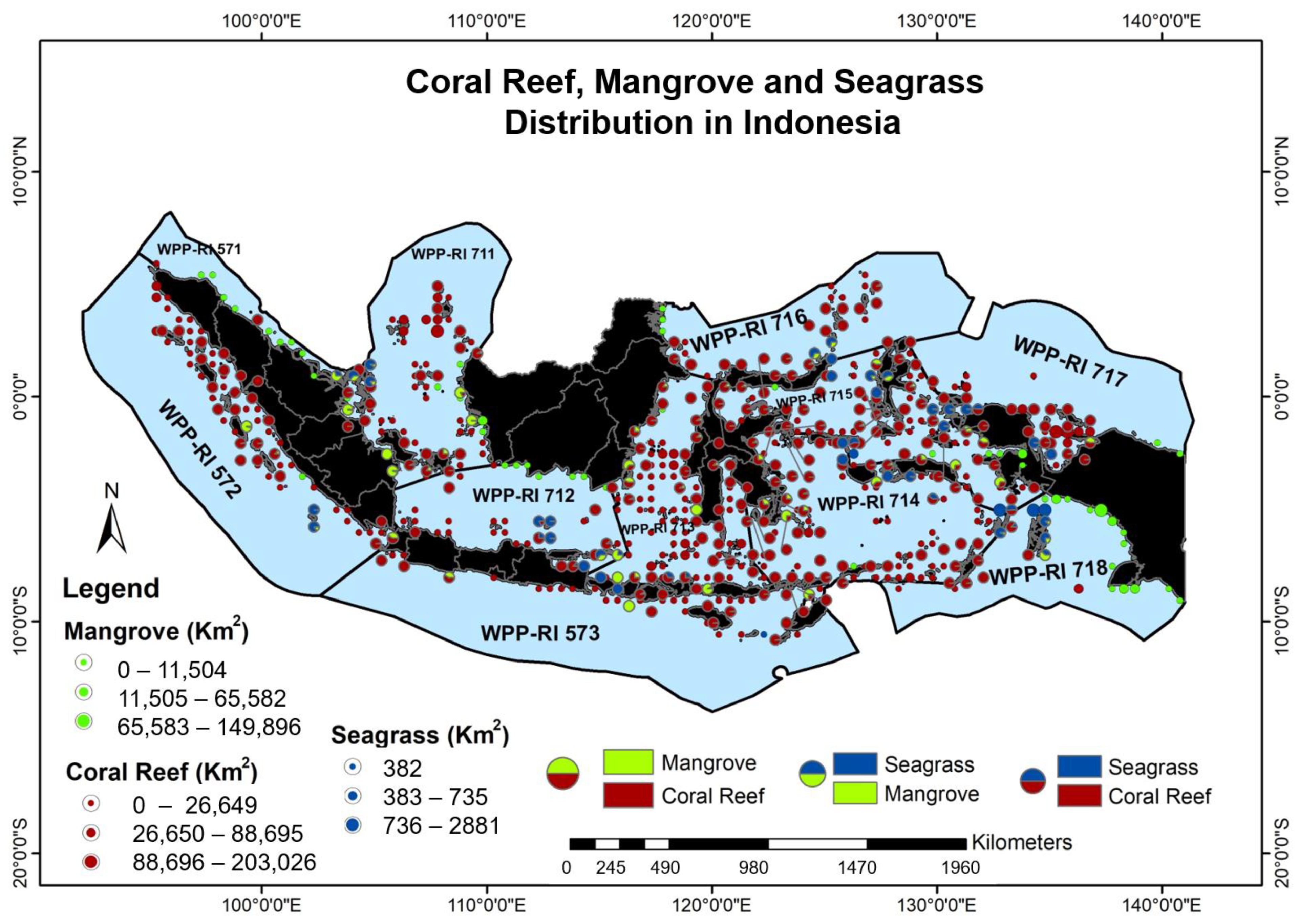
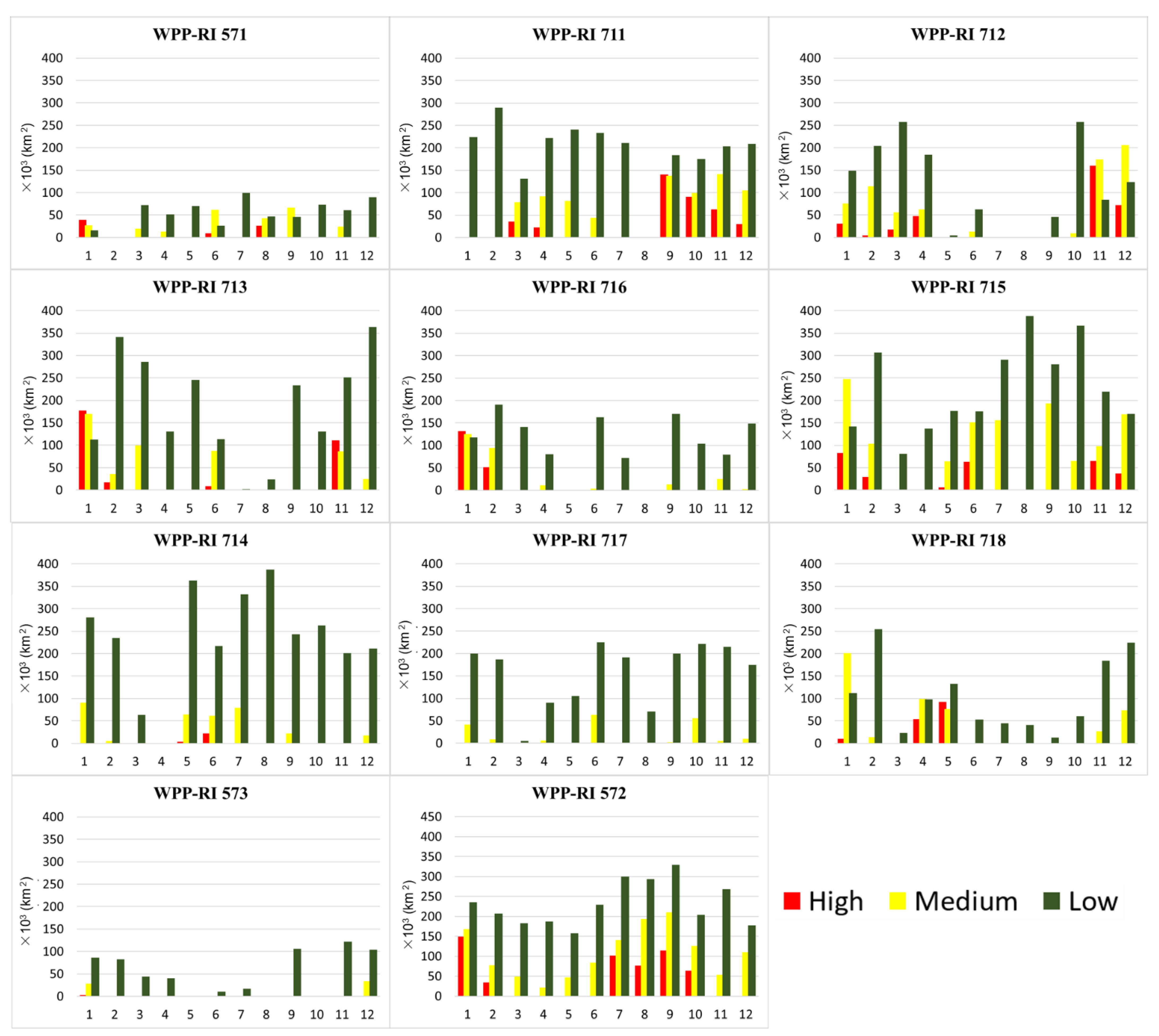
2.2. Indonesian Blue Carbon and Fisheries Management Area

Indonesia, one of the countries with the largest blue carbon ecosystem globally, was selected as the study area for this research. The blue carbon ecosystems studied include mangrove, seagrass, and coral reef ecosystems based on the UNEP-WCMC data. The mangrove, seagrass, and coral reef ecosystems spread throughout Indonesian waters divided based on the Fisheries Management Area of Indonesia Republic (WPP-RI) to facilitate analysis and evaluation (Figure 1).
WPP-RI is a management area used for fishing. It comprises deep waters, archipelagic waters, territorial seas, exclusive economic zones, and additional zones. According to the Regulation of the Minister of Maritime Affairs and Fisheries of the Republic of Indonesia Number 18/PERMENKP/2014 Article 2 [59], WPP-RI is divided into the following 11 fisheries management areas:
  • WPP-RI 571: Includes the waters of the Malacca Strait and the Andaman Sea.
  • WPP-RI 572: Includes the waters of the Indian Ocean west of Sumatra and the Sunda Strait.
  • WPP-RI 573: Includes the waters of the Indian Ocean south of Java to the south of Nusa Tenggara, the Savu Sea, and the western Timor Sea.
  • WPP-RI 711: Includes the waters of the Karimata Strait, Natuna Sea, and the South China Sea.
  • WPP-RI 712: Includes the waters of the Java Sea.
  • WPP-RI 713: Includes the waters of the Makassar Strait, Bone Bay, Flores Sea, and the Bali Sea.
  • WPP-RI 714: Includes the waters of Tolo Bay and Banda Se.
  • WPP-RI 715: Includes the waters of Tomini Bay, Maluku Sea, Halmahera Sea, Seram Sea, and Berau Bay.
  • WPP-RI 716: Includes the waters of the Sulawesi Sea and northern Halmahera Island.
  • WPP-RI 717: Includes the waters of Cendrawasih Bay and the Pacific Ocean.
  • WPP-RI 718: Includes the waters of the Aru Sea, Arafuru Sea, and the East Timor Sea.
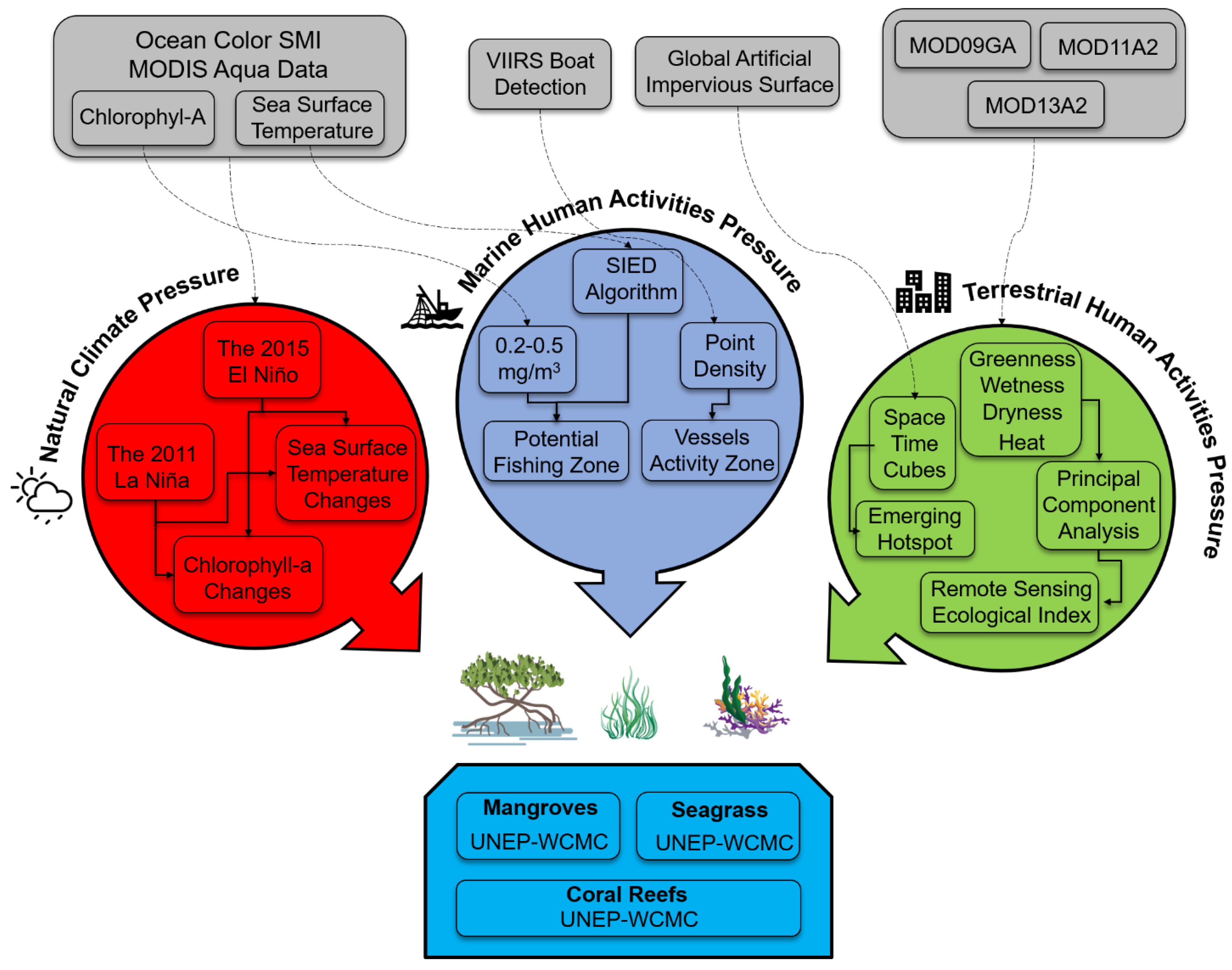
2.3. Methodology

The potential disturbances in the blue carbon ecosystem are divided into three main parts: natural climate pressure, marine human activity pressure, and terrestrial human activity pressure (Figure 2).

2.3.1. Marine Human Activity Pressure

Potential fishing zone (PFZ) was assessed using chlorophyll-a data with a range of 0.2–0.5 mg/m3 [75] and SST using the single-image edge detection algorithm [76] with a threshold of 0.5 °C [75] that subsequently produced a thermal front. Afterward, the chlorophyll-a and SST data for each month were overlaid to generate the potential fishing points, which were then averaged to obtain results for 2018. Subsequently, modeling and classification of the points were conducted based on the density of potential fishing points, divided into very low, low, medium, high, and very high classes.
Vessel activity zone (VAZ) processing used VBD data [64] with a temporal resolution of one month from January to December 2018. Initially, raster data were converted into vector format to produce a monthly point distribution of ships in the Indonesian waters. This distribution was then averaged to obtain results for 2018. Later, VAZs were classified based on the vessel density per area, divided into very low, low, medium, high, and very high classes. Finally, PFZ and VAZ were overlaid with the Indonesian blue carbon ecosystem data to produce a map of fishing effectiveness and its impact on the blue carbon ecosystem. The map comprised of nine classes, i.e., high productivity and high blue-carbon risk, moderate productivity and moderate blue-carbon risk, low productivity and low blue-carbon risk, overexploitation and high blue-carbon risk, overexploitation and medium blue carbon risk, under exploitation and moderate blue carbon risk, under exploitation and low blue carbon risk, under exploitation and sustainable blue carbon, and sustainable blue carbon.

2.3.2. Natural Climate Pressure

The MODIS OCSMI data product [70] was used to investigate the effects of climate pressure, in terms of changes in the chlorophyll-a and SST values during the La Niña (2011) and El Niño (2015) periods, on the waters of the Indonesian blue carbon ecosystem [77]. Chlorophyll-a and SST data were initially selected based on La Niña, normal (2013), and El Niño periods referring to El Niño Southern Oscillation (ENSO) data. Later, the changes in the chlorophyll-a were observed by calculating their differences during the three periods. SST changes were calculated using the same procedure. Furthermore, an overlay analysis was conducted on the blue carbon ecosystem data and the SST and chlorophyll-a differences to observe the extreme changes that occurred during the three periods in each blue carbon ecosystem.

2.3.3. Terrestrial Human Activity Pressure

During the early stages of the analysis using the emerging hotspot method [78], the GAIA data product [65] with a range of 2007–2016 was processed using the spatiotemporal cube feature at a distance interval of 2 km. Subsequently, the emerging hotspots were processed to classify the increase in Indonesia’s built-up areas for ten years based on deforestation trends. During the second stage, the ecological conditions of coastal areas in 2007 and 2016 were analyzed using the risk-screening environmental indicator (RSEI) method [79]. This method evaluates four main ecological parameters (greenness, wetness, dryness, and heat). The greenness parameter was obtained based on the EVI method using the MOD13A2 data product [68]. Temperature parameters were obtained based on the LST data using the MOD11A2 data product [67]. Further, the dryness and wetness parameters were estimated based on normalized difference build-up and soil index processing and the wet index calculations using the MOD09GA data product [66]. Subsequently, the values of the four parameters were standardized and weighed using principal component analysis to obtain the RSEI [80]. Later, the difference between the 2007 and 2016 RSEI values was calculated to evaluate the ecosystem conditions’ changes over ten years. In the last stage, mangrove data for 2007 and 2016 were subtracted to obtain the deforested mangrove area. Furthermore, emerging hotspots in built areas and RSEI changes were overlaid on the acquired deforested mangrove areas.

3. Results

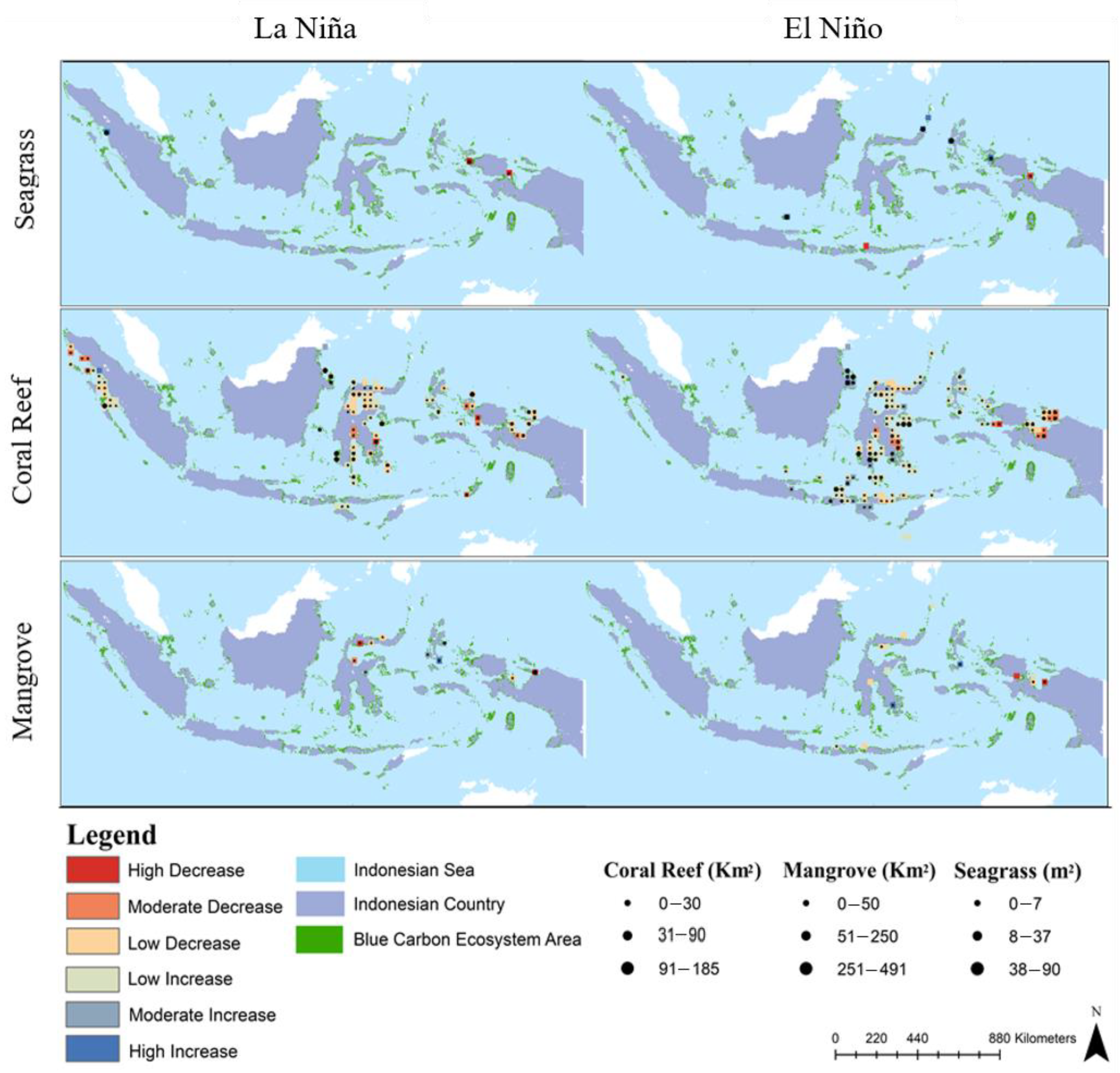
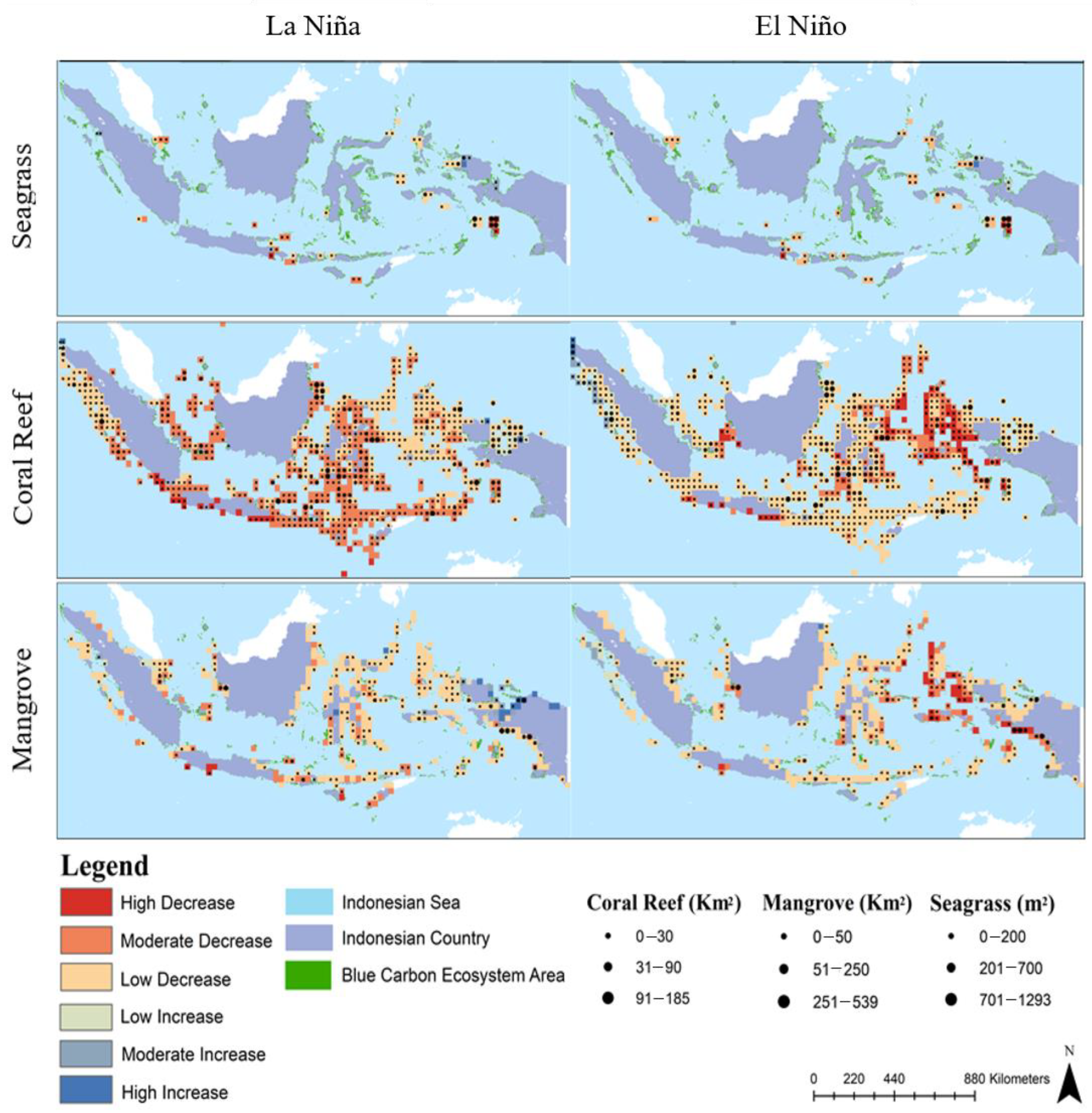
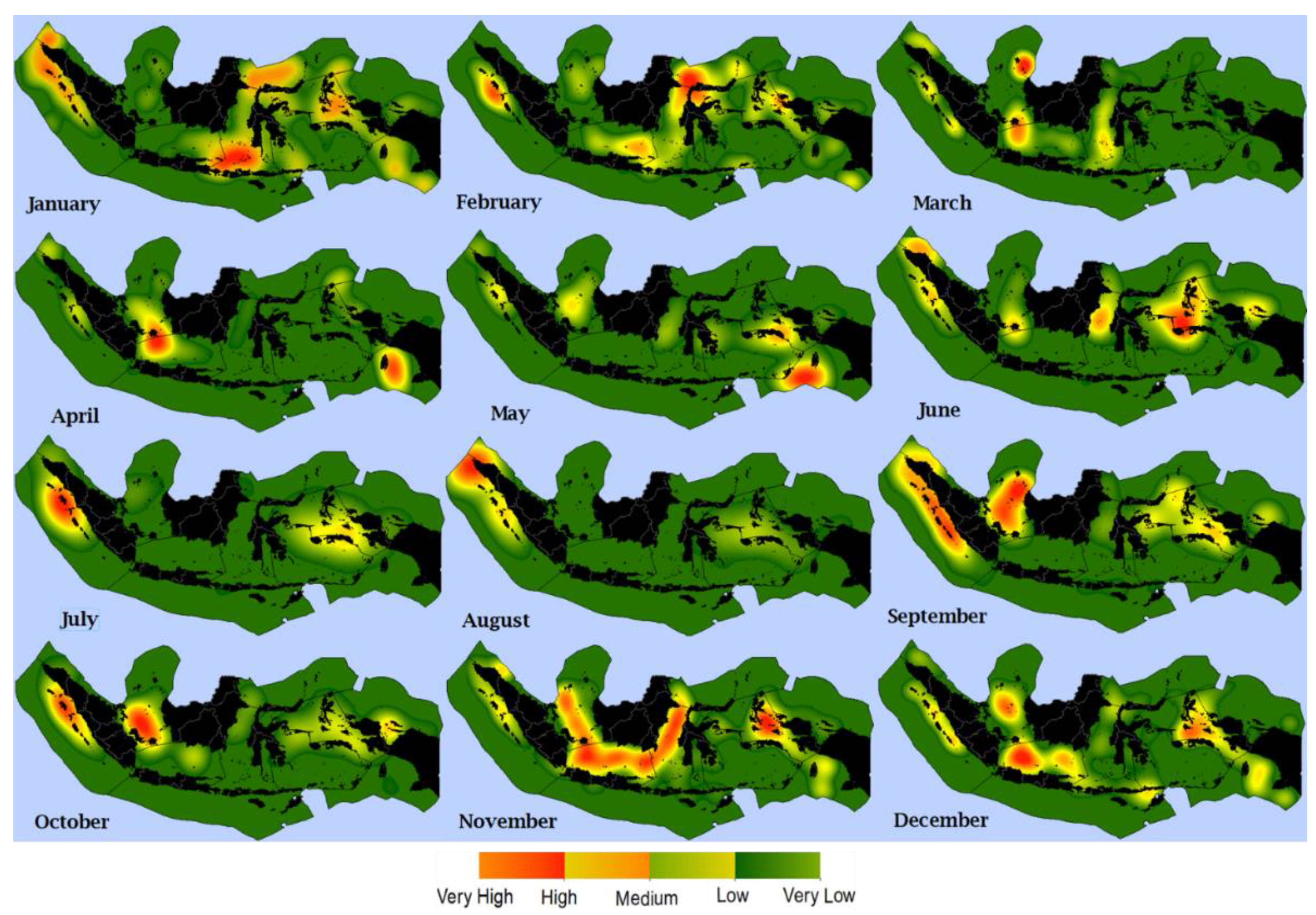
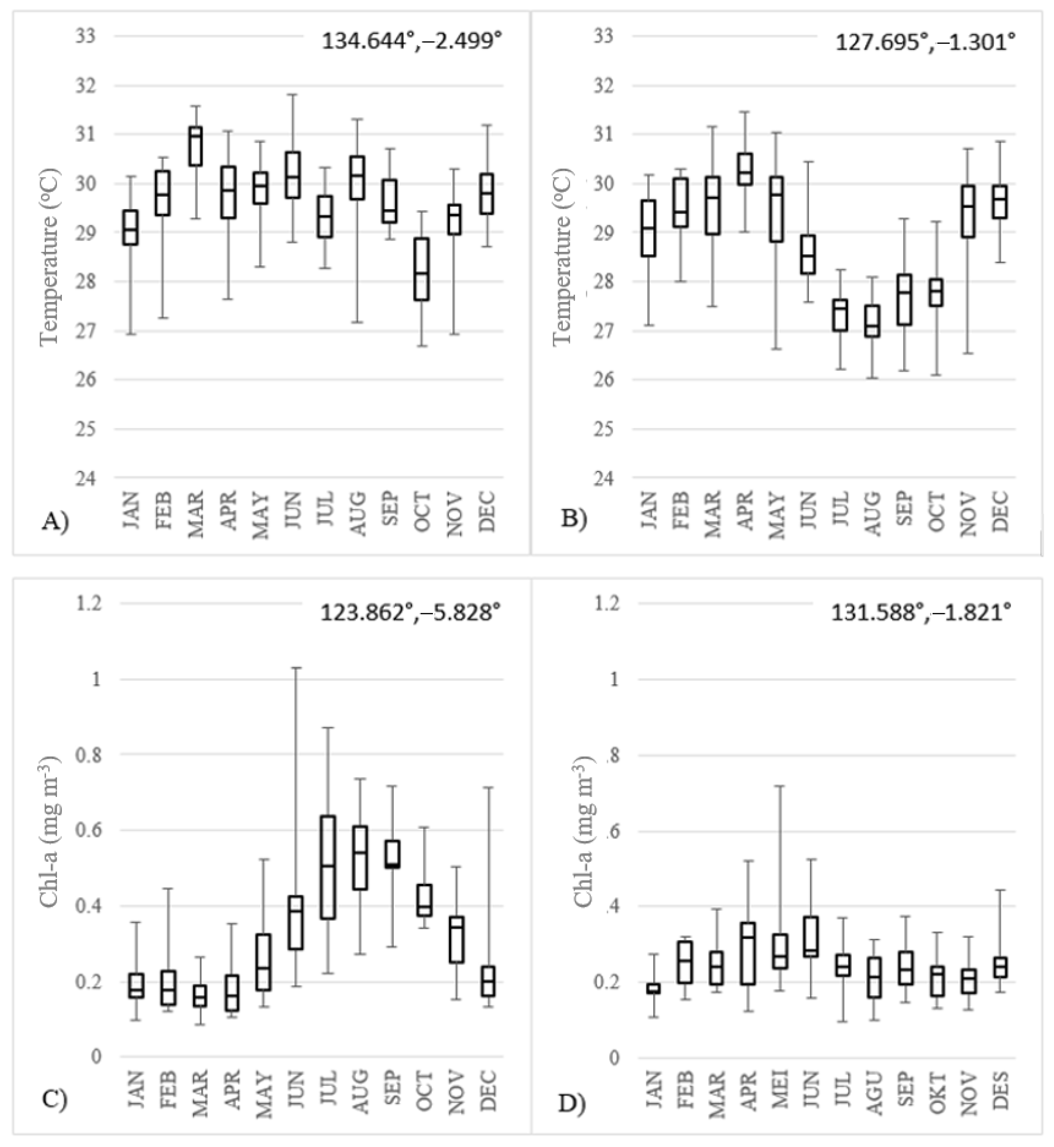
3.1. Chlorophyll-a and SST Variability during the 2011 La Niña and the 2015 El Niño Periods

Changes in chlorophyll-a during the 2011 La Niña and the 2015 El Niño periods were divided into six classes: high reduction with a range of −1 mg/m3 to −0.5 mg/m3, −0.49 mg/m3 to −0.50 mg/m3, and −0.2 mg/m3 for moderate decreases, −0.19 mg/m3 to 0 mg/m3 for low decreases, 0 mg/m3 to 0.06 mg/m3 for low increases, 0.07 mg/m3 to 0.1 mg/m3 for moderate increases, and 0.11 mg/m3 to 0.5 mg/m3 for high increases (Figure 3). The chlorophyll-a concentration significantly increased during the El Niño phenomenon in WPP-RI 714. Moreover, the chlorophyll-a concentration significantly decreased during the La Niña phenomenon in WPP-RI 715. Particularly in seagrass ecosystems, the chlorophyll-a concentration decreased during the La Niña years in WPP-RI 717. It increased during the El Niño years in WPP-RI 715.
In the coral reef ecosystems, the chlorophyll-a concentration decreased during the La Niña years in WPP-RI 572 and WPP-RI 715. In contrast, it increased during the El Niño years in WPP-RI 716 and WPP-RI 713. In the mangrove ecosystems, the chlorophyll-a concentration decreased during La Niña in WPP-RI 715. It increased during El Niño in WPP-RI 714. Changes in the SST values during La Niña and El Niño were divided into six classes: high reduction with a range of −0.5 to −0.3 °C and −0.29 to −0.1 °C for moderate decreases, −0.09 to 0 °C for low decreases, 0 to 0.5 °C for low increases, 0.51 to 0.7 °C for moderate increases, and 0.71 to 1.2 °C for high increases (Figure 4). SST significantly increased during the La Niña phenomenon in WPP-RI 717. In contrast, it significantly decreased during the El Niño phenomenon in WPP-RI 715. In the seagrass ecosystem, SST increased during La Niña in WPP-RI 572 and WPP-RI 715 and decreased during El Niño in WPP-RI 718. In the coral reef ecosystems, SST increased during the La Niña years in WPP-RI 572 and WPP-RI 717, while it decreased during the El Niño years in WPP-RI 715. In the mangrove ecosystems, SST increased during La Niña in WPP-RI 717 and decreased during El Niño in WPP-RI 715 and WPP-RI 718.

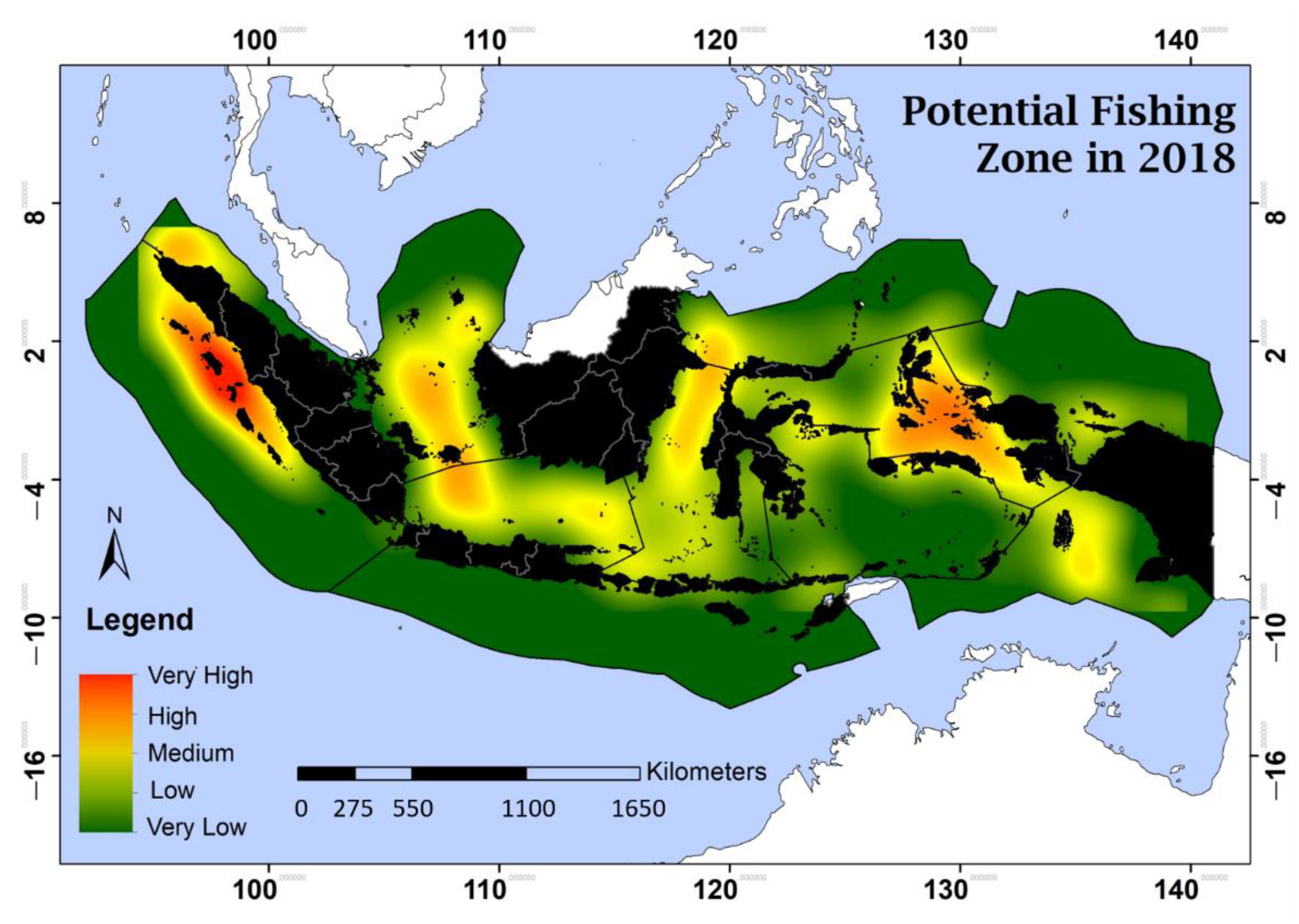
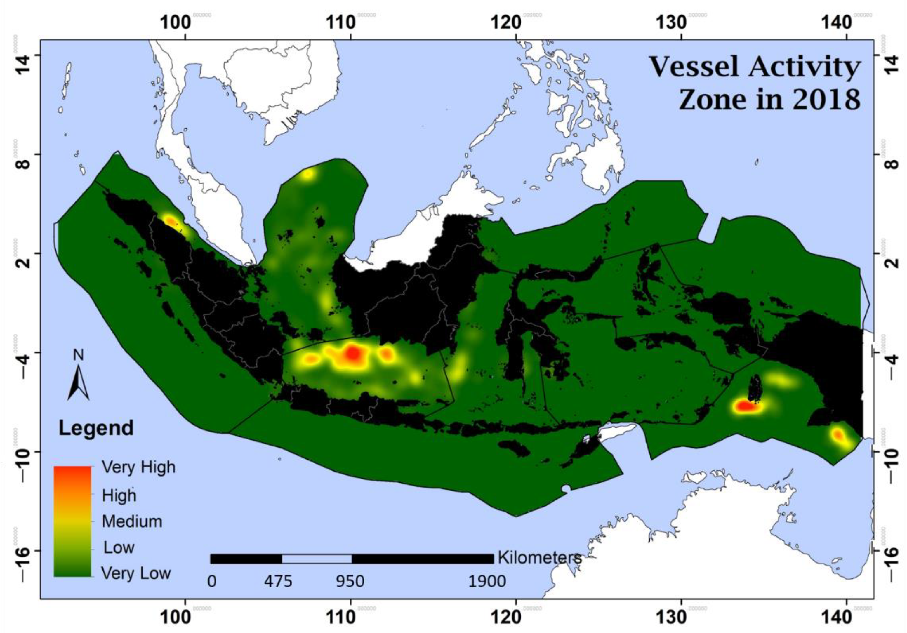
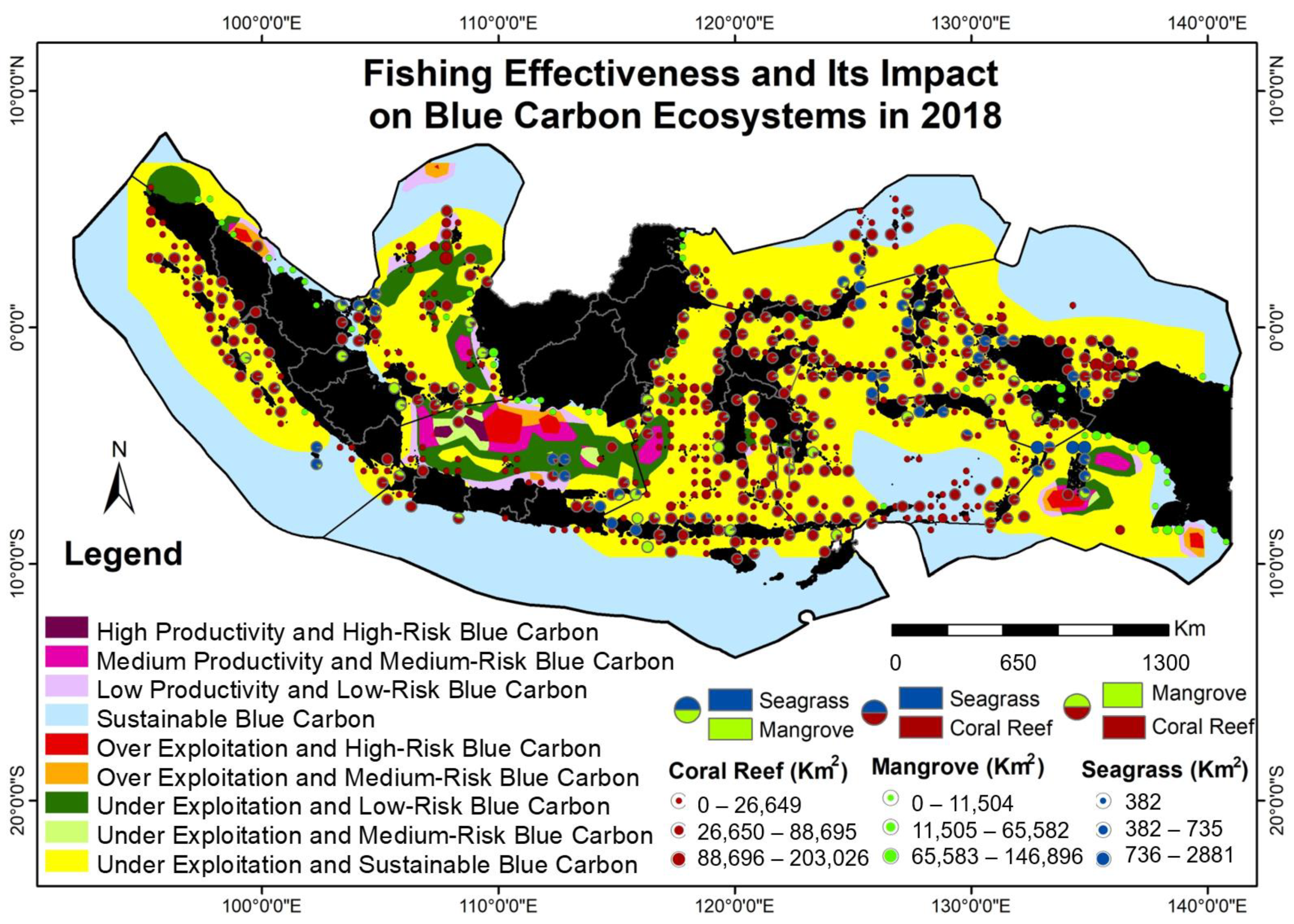
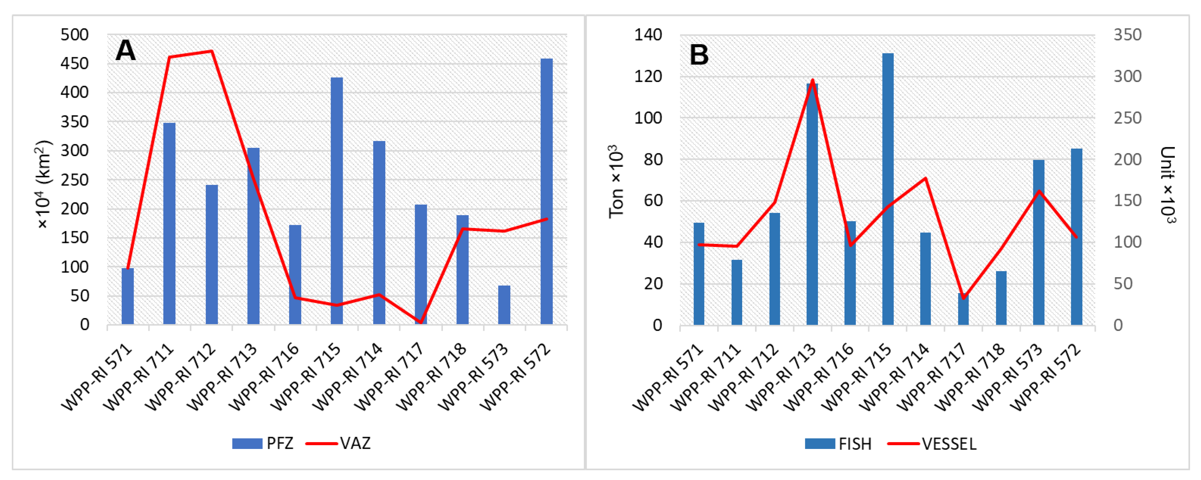
3.2. Potential Fishing Zone and Vessel Activity Zone

In 2018, the PFZ in Indonesia was divided into five classes: very low, low, medium, high, and very high, and the location of each class varied monthly and was relatively dynamic throughout the year (Figure 5). In Figure 5, the location of each PFZ class has been given concerning the WPP zones shown in Figure 1. A high PFZ was found in January, June, and August in WPP-RI 571, in March–April, and September–December in WPP-RI 711. Further, a high PFZ was found in January–April and November–December in WPP-RI 712, January–February, June, and November in WPP-RI 713, and only in January–February in WPP-RI 716.
A high PFZ was found in January–February, May–June, and November–December in WPP-RI 715, only in May–June in WPP-RI 714, in January and April–May in WPP-RI 718, only in January in WPP-RI 573, and in January–February, and July–October in WPP-RI 572. However, in WPP-RI 717, no high PFZ was observed.
Figure 6 shows that WPP-RI 572 had the largest PFZ area, whereas WPP-RI 573 had the smallest PFZ area.
Figure 6 shows that WPP-RI 712, WPP-RI 713, WPP-RI 716, and WPP-RI 715 showed medium–high potential periods from September to April with peaks in January–December. Other fish catch potential dynamics patterns of medium-high potential from July to December, with peaks in September, were observed in WPP-RI 711 and WPP-RI 572. The potential dynamics patterns were not observed comprehensively in other WPP-RIs.
The average fishing potential in Indonesian waters in 2018 was generally dominated by medium to high classes in all areas of WPP-RI, except WPP-RI 573, WPP-RI 714, and WPP-RI 717, as shown in Figure 7.
Regions with a high monthly average potential dominance during 2018 were WPP-RI 572 and WPP-RI 715. Moreover, WPP-RI 711, WPP-RI 712, and WPP-RI 718 showed medium potential. VAZ in Indonesia in 2018 was divided into three classes: low, medium, and high, and the location of each class varied monthly, particularly in WPP-RI 571, WPP-RI 712, and WPP-RI 718 (Figure 8). WPP-RI 571, with high VAZ, was observed in February–May and November–December. A high VAZ was observed every month in WPP-RI 712 from January to December and in WPP-RI 718 in January–April and July–December.
Figure 9 shows that the average ship activity in 2018 was concentrated only in WPP-RI 571, WPP-RI 711, WPP-RI 712, WPP-RI 713, and WPP-RI 718. In particular, medium–high VAZ was concentrated only in WPP-RI 571, WPP-RI 712, and WPP-RI 718.
The acquired PFZ and VAZ results were combined with the blue carbon ecosystem distribution data to map fisheries’ effectiveness and blue carbon ecosystem threats. The resultant map was divided into the following nine area classes (Figure 10):
  • High productivity and high blue-carbon risk: characterized by high potential and high ship activity; thus, this area has a high fishery yield. However, the blue carbon ecosystem around this area faces high pressures due to the high ship activity.
  • Moderate productivity and moderate blue-carbon risk: these areas have a moderate level of fisheries potential and moderate ship activity; therefore, these areas have moderate fishery production, and the blue carbon ecosystem experiences moderate levels of damage.
  • Low productivity and low blue-carbon risk: these areas have a low level of fisheries potential and low ship activity; thus, they have low fishery production yields and experience low levels of blue carbon ecosystem damages.
  • Overexploitation and high blue-carbon risk: these areas have a low-to-moderate level of fishery potential but a high level of ship activity; thus, these areas are overexploited and have high levels of damage to the blue carbon ecosystem.
  • Overexploitation and medium blue carbon risk: these areas have a low fishery potential but a moderate level of ship activity; thus, these areas are overexploited and have moderate levels of damages to the blue carbon ecosystem.
  • Under exploitation and moderate blue carbon risk: these areas have a high fishery potential but a moderate ship activity. Therefore, these areas are less exploited and have moderate levels of damages to the blue carbon ecosystems.
  • Under exploitation and low blue carbon risk: these areas have a moderate level of fishery potential but a low level of ship activity; therefore, these areas are less exploited and have low levels of damages to the blue carbon ecosystems.
  • Under exploitation and sustainable blue carbon: these areas have a low to a high level of fishery potential but minimal ship activity; thus, these areas are less exploited, and the blue carbon ecosystem is relatively sustained.
  • Sustainable blue carbon: the areas belonging to this class have a very low fishery potential and ship activity level. Thus, the blue carbon ecosystems are relatively maintained.
Figure 10 shows that the effectiveness of fishing and its impact on the blue carbon ecosystems in Indonesia were mostly underexploited and sustainable in most WPP-RIs. However, the overexploitation and high blue carbon risk classes, which were of major concern, were observed only in WPP-RI 571, WPP-RI 712, WPP-RI 711, WPP-RI 713, and WPP-RI 718.

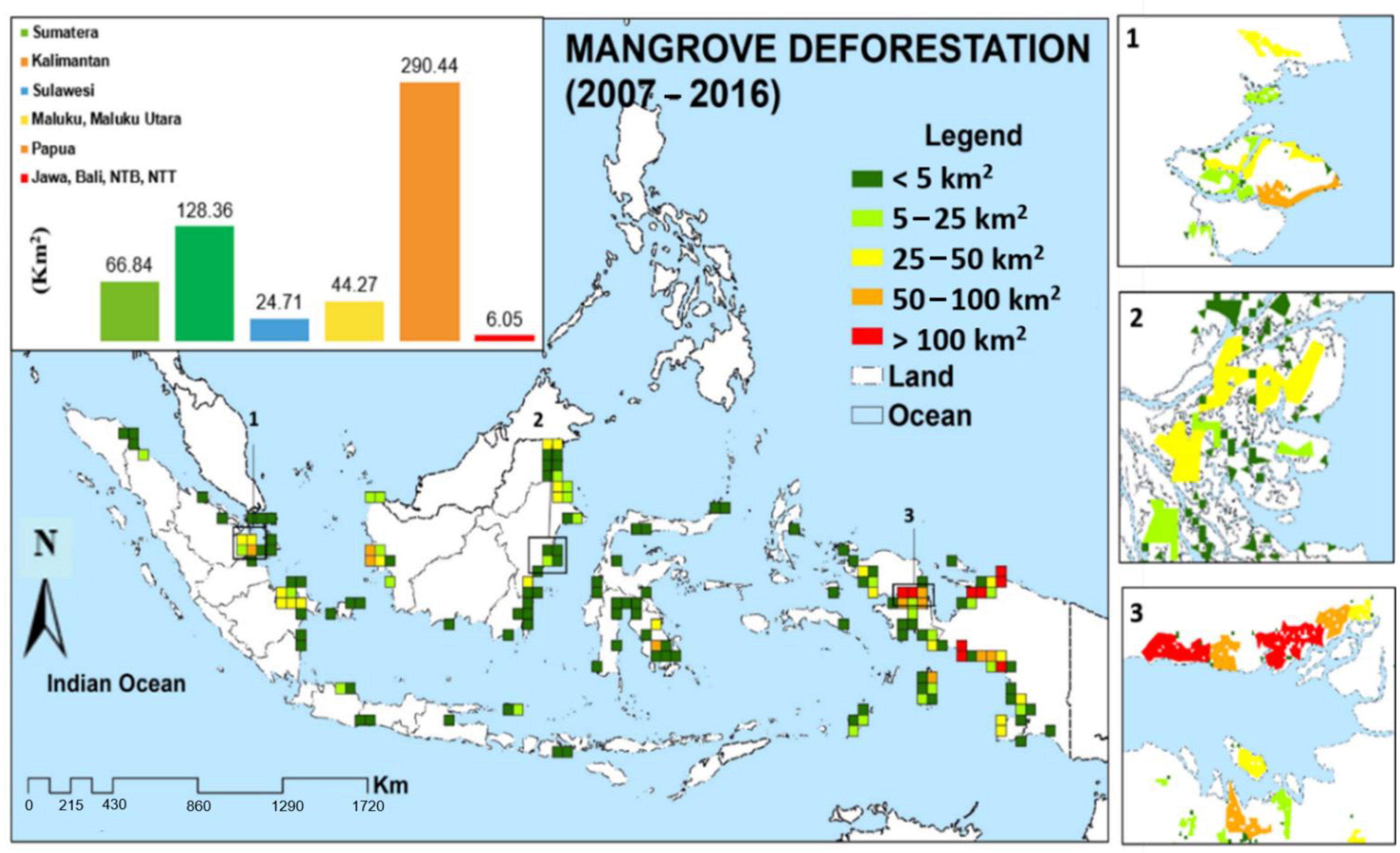
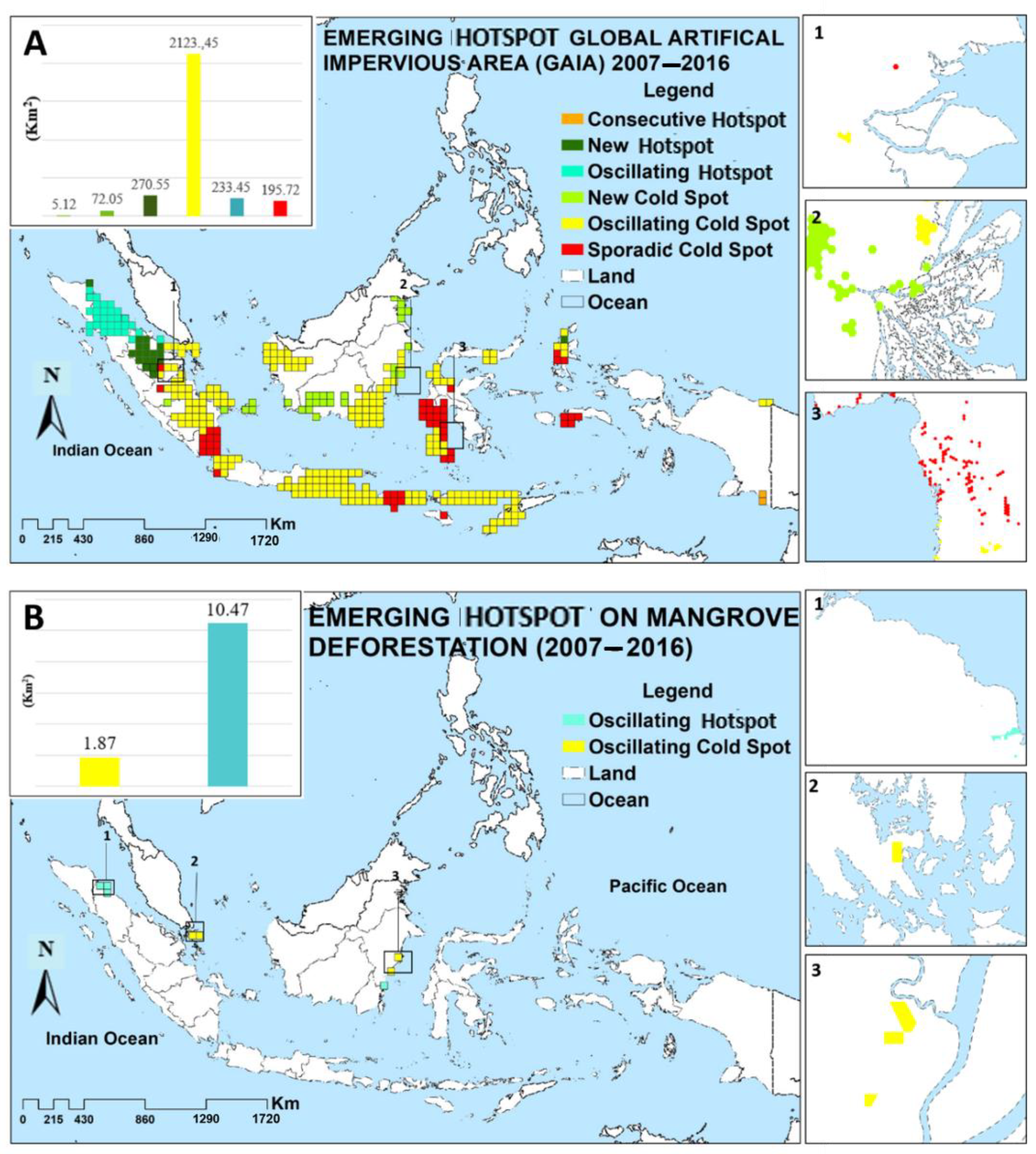
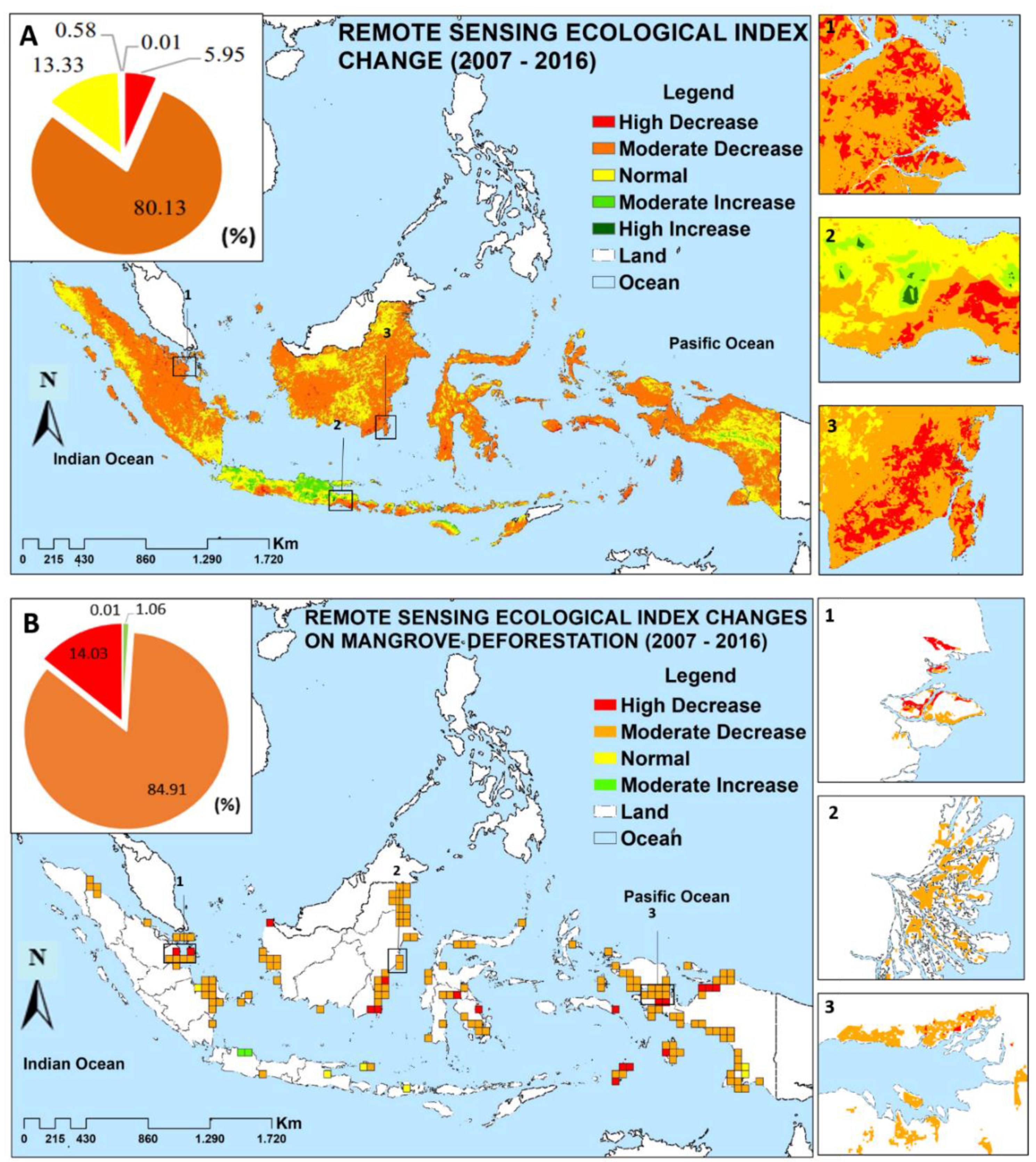
3.3. Coastal Urbanization and RSEI Changes on Deforested Mangrove Forests

The results of mangrove deforestation based on the GMW data from 2007 to 2016 included five deforestation classes: <5, 5–25, 25–50, 50–100, and >100 km2 (Figure 11). Based on visual observations, mangrove deforestation with <500 ha was evenly distributed in every region (Kalimantan, Sumatra, Sulawesi, Maluku, and Java). Mangrove deforestation in the class range of 5–25, 25–50, and 50–100 km2 primarily occurred in Kalimantan and Papua, Sumatra and Kalimantan, and Papua, respectively.
Papua showed the largest mangrove deforestation area (290.44 km2). In contrast, Java, Bali, West Nusa Tenggara, and East Nusa Tenggara showed the smallest deforestation area (6.05 km2). The proportion of deforestation areas in Kalimantan, Sumatra, Maluku, North Maluku, and Sulawesi was 128.36, 66.84, 44.27, and 24.71 km2, respectively.
The GAIA data processing results for 2007–2016 were classified into six classes of incident trends: consecutive hotspots, new hotspots, oscillating hotspots, new cold spots, oscillating cold spots, and sporadic cold spots, as shown in Figure 12. Oscillating cold spots, areas with periodic urban growth and a below-average frequency value, had the largest area (2123.45 km2). Consecutive hotspot class, characterized by successive urban growth and an above-average frequency, covered an area of 5.12 km2. The new cold spot class, characterized by areas that witnessed urban growth recently and characterized by below-average frequency, covered an area of 72.05 km2. The new hotspot class, with areas that witnessed urban growth recently and an above-average frequency, covered an area of 270.55 km2. The oscillating hotspot class, characterized by periodic urban growth and an above-average frequency, covered an area of 233.48 km2. Moreover, the sporadic cold spot class, characterized by random urban growth and a below-average, had an area of 195.72 km2.
Emerging hotspots on mangrove deforestation were found in only two classes: oscillating hotspots that dominated North Sumatra and cold spots that dominated the East Kalimantan and Riau Islands (Figure 12B). The areas covered by the oscillating hot and cold spot classes were 10.47 and 1.87 km2, respectively.
Based on the RSEI changes during 2007–2016, five changes were obtained: high decrease, moderate decrease, normal, moderate increase, and high increase (Figure 13).
In all regions of Indonesia, the most dominant changes in the RSEI during 2007–2016 occurred in the medium decrease class (80.13%). Further, the RSEI changes in the normal, high decrease, and moderate improvement classes were 13.33, 5.95, and 0.58%, respectively; however, RSEI changes were almost negligible in the high improvement class (0.01%). Moreover, the RSEI changes in the deforested mangrove areas occurred only in four classes: moderate increase (0.01%), normal (0.58%), medium decrease (84.91%), and high decrease (14.01%).

4. Discussion

The main results presented in the third section are classified based on three potential pressures and briefly summarized in Table 3. These findings were discussed further in subsection four.

4.1. Impact of the 2011 La Niña and 2015 El Niño Phenomena on the Blue Carbon Ecosystems in Indonesia

Indonesian waters experience a decrease in the chlorophyll-a concentration and an increase in the SST during La Niña. Furthermore, during the El Niño phenomenon, the dominant chlorophyll-a value increased, and the dominant SST decreased (Figure 14). Seprianto [81] stated that the value of chlorophyll-a in Karimun Jawa waters increased during the El Niño phenomenon and decreased during the La Niña phenomenon. Similarly, other previous studies reported that the SST temporarily decreased during the El Niño phenomenon, while it increased during the La Niña phenomenon [26,82]. This occurs because ocean–atmosphere climate interactions, such as those resulting from the ENSO, affect the sea level, SST, air temperature, chlorophyll-a, and upwelling intensity. During the El Niño period, the upwelling intensity increased, followed by an increase in the chlorophyll-a concentration; in contrast, during the La Niña period, the upwelling intensity decreased followed by a decrease in the chlorophyll-a concentration [26,82,83,84,85].
The SST increased significantly in the blue carbon ecosystem in 2011 (La Niña), with an average value of 29.6 °C and the highest value of 31.8 °C in June. Moreover, the SST decreased significantly in 2015 (El Niño), with an average value of 28.8 °C and the lowest value of 26 °C in August. These results were confirmed by the observations by Nabilah [82], who conducted research on the Java Sea and indicated that during El Niño, the SST was in the range of 27–28 °C with an average value of 27.71 °C; moreover, during La Niña, the SST was in the range of 29–30 °C with an average value of 29.06 °C.
The chlorophyll-a concentration significantly increased in the blue carbon ecosystem in 2015 (El Niño), with the highest value of 1.02 mg m−3 in June and an average value of 0.3 mg m−3. However, in 2011 (La Niña), chlorophyll-a concentration decreased significantly with an average value of 0.2 mg m−3 and a lowest value of 0.09 mg m−3 in July. These results were confirmed by Sari [86], who conducted similar research in Tomini Bay, Sulawesi, and found that during El Niño, the chlorophyll-a concentration increased to >0.1 mg m−3, while during La Niña, it decreased to <0.1 mg m−3.
Significant changes in the SST and chlorophyll-a concentrations considerably affect the vulnerable and sensitive blue carbon ecosystems [87]. Heron [88] showed that corals in coral reef ecosystems can experience bleaching when exposed to temperatures of 1 °C above normal. Several studies on mangrove ecosystems have revealed that climatic factors significantly influence the development of mangroves and their ability to store carbon [89,90]. Moreover, other studies on seagrass ecosystems separately reported the threats to and mass death of seagrass beds triggered by hypersalinity and acidification caused by increased SSTs [91,92].

4.2. Comparison of the Potential Fishing Zone and Vessel Activity Zone with Production Data and the Number of Fishing Vessels of the Ministry of Maritime Affairs and Fisheries

In general, the average fishing potential in Indonesian waters in 2018 was dominated by classes with medium to high potential levels covering almost all WPP-RIs, except WPP-RI 573, WPP-RI 714, and WPP-RI 717. Insanu [93] reported that in the waters of the Mahakam Delta and Makassar Strait, the high fishing zone occurs south of the Mahakam Delta, and in the middle of the Makassar Strait. Furthermore, Suhadha [75] reported water areas with high fishing potential in WPP-RI 715 and WPP-RI 712. Similar patterns were also observed according to the PFZ in Indonesian waters, and the results of the Institute of Aeronautics and Space Indonesia (SPBN lapan.go.id).
The high level of PFZ is attributed to the location of the mesotrophic area, which has a sufficiently high chlorophyll-a concentration; therefore, the seawaters of this PFZ has moderate biological productivity, sufficient water quality, and high nutrient richness [75,94,95]. PFZ is also influenced by temperature. Insanu [93] reported that high potential fishing areas have SSTs ranging from 27 to 30 °C and high chlorophyll-a concentrations [75,96,97]. Based on our results, VAZs in Indonesia in 2018 were dominant in WPP-RI 712, WPP-RI 571, and WPP-RI 718. This was consistent with the findings by Hsu [71] and Lumban [98], who reported that VAZ was dominant because it is used as a fishing ground and a shipping area. In particular, WPP-RI 718 and WPP-RI 712, which are located around the Sunda Strait, are gateways for shipping vessels used for economic trade activities with China and other countries [99].
Figure 15 shows the comparison between the results of our study and the data from the Ministry of Maritime Affairs and Fisheries (MMAF a.k.a. KKP) The distribution of potential fish catch areas has not been represented by the distribution of fishery production in each WPP-RI. This is because most areas were underexploited. Further, the distribution of the VAZ vessels was not uniform with the number of vessels based on the MMAF data. This is because VAZ is a general vessel, while MMAF provides information on the fishing vessel data.
In WPP-R1 715, WPP-R1 714, WPP-R1 717, and WPP-RI 572, data from both sources showed an under-exploitation status, with the MMAF data showing lower number of production and fishing vessels in the above-mentioned areas than other areas, and the results of our study showed that these areas had high fishing potential. WPP-R1 711, WPP-R1 712, WPP-RI 713, and WPP-RI 573 indicated overexploitation based on the high production level and number of fishing vessels based on the MMAF data; additionally, our study results showed low fishing potential and high ship activity. These observations were consistent with the findings by Darmawan [100], who stated that the high damages in WPP-RI 712 occurred due to waste pollution, and thus, coral reefs were not preserved. Noviyanti [101] reported that mangroves were damaged in this area. Another study stated that coral reef damage in WPP-RI 713 was reported to be caused by tourism and fishing activities that were not environmentally friendly [102]. Syukur [103] also reported damages to seagrass beds in WPP-RI 713 on the island of Lombok that were caused by overexploitation.

4.3. Mangrove Deforestation and the Decline in the RSEI in Indonesia during 2007–2016

The rate of mangrove deforestation in Indonesia during 2007–2016 was 56.068 km2/year. A previous study has shown that the rate of mangrove deforestation in Indonesia during the 2000–2012 was 57.74 km2/year [104]. Therefore, mangrove deforestation has gradually decreased, despite the percentage decrease of only approximately 1.68 km2 or 2.9% of the total. Coastal urbanization contributes only 12.34 km2 or 2.2% [49], indicating that urban growth is not a significant factor causing mangrove deforestation in Indonesia.
The largest mangrove deforestation incident during 2007–2016 occurred in the Papua region (290.44 km2). A study conducted on the coast of the South Manokwari District, particularly at Wasti Sowi IV Lake, indicated a decrease in the mangrove forest area from 2006 to 2018 because of the use of mangrove plants as building construction materials, fuel wood, medicinal resources, and other essential supplies [105]. Mangrove deforestation due to urban expansion marginally contributes to the total mangrove deforestation and occurs in North Sumatra, East Kalimantan, and the Riau Islands. Among these, development in the coastal areas of East Kalimantan has been conducted since 2007 to develop the area as a tourist destination [106].
In this study, correlation analysis was conducted using 100 samples randomly collected in intersecting regions of deforested mangrove forest and RSEI decline. Subsequently, a correlation coefficient of 0.72 was obtained (Figure 16), indicating a strong relationship between the two variables [107]. Thus, the RSEI can be used to measure the level of damage in deforested mangrove areas.

4.4. Study Limitations

This study is limited by several factors, including topic limitations, data availability, analytical methods, and data validation. Regarding topic limitations, the blue carbon ecosystem research did not include salt marsh ecosystems due to the lack of distribution data of such ecosystems in the Indonesian regions. Further, while investigating the pressures due to climatic factors, natural phenomena were considered based on only the conditions of the extreme La Niña and El Niño phenomena. In addition, only changes that occurred in two oceanographic parameters of the sea (SST and chlorophyll-a) were considered. Regarding data availability, several gaps existed with incomplete monthly datasets for both SS and chlorophyll-a. During data preprocessing, no data gap-filling or interpolation processes were conducted to obtain a comprehensive understanding.
While investigating the potential stresses due to human activities in the sea, the distribution model of fishing potential used only oceanographic parameters of SST and chlorophyll-a, while the criteria for the range of values of these two parameters were used only for pelagic fish species. The VBD data included the VAZ distribution, which was general vessel activity, and did not refer to the type of vessels specifically used for fishing activities. In addition, the classification of monthly fishing potential and vessel activity referred to the range of monthly values, instead of the absolute values used as standards.
Furthermore, the investigation of pressures due to human activities in coastal areas only analyzed the blue carbon areas of mangrove ecosystems. This was because of the unavailability of multi-temporal seagrass and coral reef data that could assist in further analyzing the changes. In addition, the seagrass and coral reef ecosystems were not assessed during the analysis using the hotspot method and RSEI because of difficulty of access of these ecosystems through the method based on land area data. Moreover, all data analyses in this study relied only on previous similar studies, reliable literature, and secondary data to validate the accuracy of the acquired results. This was because of the limitations of comparative data and limitations in conducting field surveys in the selected large study area.

4.5. Future Research Directives

Several future research avenues can be explored further to supplement and improve the accuracy of the results acquired in this study. The analysis of climate effects can apply various methods, such as the data interpolating empirical orthogonal functions [108] and fixed rank kriging [109] to fill the gaps in the chlorophyll-a and SST data occurring due to cloud cover. In addition, several other climatic phenomena, such as typhoons [110], storms [111,112], heat waves [113], and droughts [114] have been reported to significantly affect the blue carbon ecosystems; thus, these climatic events should be comprehensively studied. Additionally, physiochemical parameters, such as salinity [115,116,117], total suspended solids [118], and colored dissolved organic matter [119], that can be extracted through remote sensing can be used to build more complex and comprehensive models. Moreover, several studies have acquired data directly in the field to determine the actual conditions and to validate the acquired results [120,121].
During the analysis of pressure due to fishery activities, PFZ can be modeled using more parameters, such as TSS, sea surface height [122], sea surface salinity [123,124], and merged sea level of anomaly [125]; additionally, the PFZ can be quantitatively converted to the potential fish catch weight per area. Another important research consideration is the classification of the VBD data using specific algorithms to separate fishing vessels from other vessel types [71,126]. In addition, future research can formulate and recommend ideal fishing zones and blue carbon conservation zones to mutually encourage fishing productivity while preserving ecosystems to support the implementation of a blue economy [127].
The current data on the distribution of seagrass and coral reefs regarding land disturbances are still limited. However, several mapping methods based on remote sensing have been developed and proven to be able to map these ecosystems efficiently [128]. Future research should focus on monitoring the quantity and quality of blue carbon ecosystems in Indonesia by utilizing a proven methodology using basic data for conserving coastal and marine ecosystems by developing global climate change mitigation strategies and exploring the potential for ecotourism in the tropical regions [128,129]. In addition, other spatial data products, such as nighttime lights, population, and accessibility, can be integrated to develop an indicator of human activity pressure in coastal areas to detect potential degradation of aquatic waste [79,130].
From the perspective of maritime ecosystem conservation, this study serves as a basis that can promote the development of a spatial model of ecosystem services and threats to the blue carbon ecosystem using complex parameters and methods based on extensive data from remote sensing, cloud computing, and artificial intelligence to expand regional study areas to a global scale [34,131,132]. Furthermore, the model can be studied through not only the physical aspect of the environment but also the socio-economic aspects by involving multiple stakeholders, including a multidisciplinary research team, the government, and local residents [133].

5. Conclusions

Based on the findings of the study, we can conclude that several blue carbon ecosystems in Indonesia are threatened due to significant changes in the chlorophyll-a concentration and SST during the La Niña period (2011). During this period, 52.46 km2 of the total blue carbon ecosystem experienced a decrease in the chlorophyll-a concentration reaching −1 mg/m3, and 19.83 km2 of these ecosystems experienced an increase in the SST of up to +1.2 °C. Further, from the perspective of pressures in the sea, most blue carbon ecosystems in the Indonesian waters are underexploited and are sustainable, while WPP-RI 571, WPP-RI 712, WPP-RI 711, WPP-RI 713, and WPP-RI 718 experienced overexploitation and were included in the high-risk blue carbon class. Regarding terrestrial pressures, mangrove deforestation during 2007–2016 occurred in 560.69 km2, as confirmed by the decrease in the RSEI (84.9%). Coastal urbanization contributed to only 12.34 km2 or 2.2% of the total mangrove deforestation. Overall, this study could successfully map the potential pressures on Indonesia’s blue carbon ecosystems, which have varied geographical characteristics. The results obtained can be used as a reference for the development of habitat threat models to support the planning of conservation priority areas. Equipped with a service ecosystem model that integrates physical and socio-economic aspects, the main goals of sustainable development goals (SDGs) 2 (zero hunger), 13 (climate action), and 14 (life below water) can be achieved through simultaneous efforts to increase fisheries’ productivity, conservation, and restoration of blue carbon ecosystems based on the blue economy. In the near future, spatial data can explore further opportunities to study the food–marine biodiversity–climate nexus interaction approach to achieve a global maritime ecological balance.

Author Contributions

Conceptualization, Adam Irwansyah Fauzi and Anjar Dimara Sakti; methodology, Balqis Falah Robbani , Mita Ristiyani, Rahiska Tisa Agustin and Emi Yati; software, Balqis Falah Robbani , Mita Ristiyani and Rahiska Tisa Agustin; validation, Adam Irwansyah Fauzi, Anjar Dimara Sakti, Balqis Falah Robbani , Mita Ristiyani and Rahiska Tisa Agustin; formal analysis, Adam Irwansyah Fauzi and Anjar Dimara Sakti; investigation, Adam Irwansyah Fauzi and Anjar Dimara Sakti; resources, Balqis Falah Robbani , Mita Ristiyani, Rahiska Tisa Agustin and Emi Yati; data curation, Balqis Falah Robbani , Mita Ristiyani and Rahiska Tisa Agustin; writing—original draft preparation, Adam Irwansyah Fauzi, Balqis Falah Robbani , Mita Ristiyani and Rahiska Tisa Agustin; writing—review and editing, Adam Irwansyah Fauzi, Anjar Dimara Sakti, Nova Anika, Raden Putra, Diyanti Isnani Siregar, Budhi Agung Prasetyo, and Atriyon Julzarika; supervision, Ketut Wikantika; project administration, Muhammad Ulin Nuha; funding acquisition, Adam Irwansyah Fauzi and Muhammad Ulin Nuha. All authors have read and agreed to the published version of the manuscript.

Funding

This research was funded by Institut Teknologi Sumatera through “Hibah Penelitian ITERA 2021” grant number (No. B/496/IT9.C/PT.01.03/2021) and Capacity Building Research Program for ITB Young Scientists by the Institute of Research and Community Service, Institut Teknologi Bandung.

Institutional Review Board Statement

Not applicable.

Informed Consent Statement

Not applicable.

Data Availability Statement

The datasets generated during and/or analyzed during the current study are available from the corresponding author on reasonable request. The data used in this study were mainly provided by the institution introduced in Section 2.1. Fishing Management Zone (WPP-RI) is available at (http://pusriskel.litbang.kkp.go.id/index.php/en/data/perairan-indonesia/category/70-shape-file-laut-indonesia/; accessed on 3 February 2021). Global Mangrove Watch (GMW) data are available at (https://data.unep-wcmc.org/datasets/45; accessed on 3 March 2021). Global Distribution of Seagrasses (GDS) data are available at (https://data.unep-wcmc.org/datasets/7; accessed on 8 April 2021). Global Distribution of Coral Reefs (GDCR) data are available at (https://data.unep-wcmc.org/datasets/1; accessed on 20 March 2021). MODIS Ocean Color Standard Mapped Image data are available at (https://developers.google.com/earth-engine/datasets/catalog/NASA_OCEANDATA_MODIS-Aqua_L3SMI; accessed on 27 February 2021 from GEE). VIIRS Boat Detection data are available at (https://eogdata.mines.edu/vbd/; accessed on 12 March 2021). Global Artificial Impervious Area (GAIA) data are available at (https://developers.google.com/earth-engine/datasets/catalog/Tsinghua_FROM-GLC_GAIA_v10?hl=en#citations; accessed on 2 April 2021 from GEE). MOD09GA data are available at (https://developers.google.com/earth-engine/datasets/catalog/MODIS_006_MOD09GA?hl=en; accessed on 17 March 2021 from GEE).MOD11A2 data are available at (https://developers.google.com/earth-engine/datasets/catalog/MODIS_006_MOD11A2?hl=en; accessed on 15 March 2021 from GEE). MOD13A2 data are available at (https://developers.google.com/earth-engine/datasets/catalog/MODIS_006_MOD13A2?hl=en; accessed on 20 March 2021 from GEE).

Acknowledgments

The authors are grateful to acknowledge the support from Institut Teknologi Sumatera and Institut Teknologi Bandung. We also thank the anonymous reviewers whose critical and constructive comments greatly helped us to prepare an improved and clearer version of this paper. All persons and institutes who kindly made their data available for this research are acknowledged.

Conflicts of Interest

The authors declare no conflict of interest.

References

  1. Nellemann, C.; Corcoran, E.; Duarte, C.M.; Valdés, L.; De Young, C.; Fonseca, L.; Grimsditch, G. Blue Carbon: A Rapid Response Assessment; United Nations Environment Programme; GRID-Arendal: Arendal, Norway, 2009. [Google Scholar]
  2. Duarte, C.M.; Losada, I.J.; Hendriks, I.E.; Mazarrasa, I.; Marbà, N. The role of coastal plant communities for climate change mitigation and adaptation. Nat. Clim. Chang. 2013, 3, 961–968. [Google Scholar] [CrossRef] [Green Version]
  3. Howard, J.; Hoyt, S.; Isensee, K.; Pidgeon, E.; Telszewski, M. Coastal Blue Carbon: Methods for Assessing Carbon Stocks and Emissions Factors in Mangroves, Tidal Salt Marshes, and Seagrass Meadows. In Conservation International, Intergovernmental Oceanographic Commission of UNESCO; International Union for Conservation of Nature: Arlington, VA, USA, 2014. [Google Scholar]
  4. Bulmer, R.H.; Stephenson, F.; Jones, H.F.E.; Townsend, M.; Hillman, J.R.; Schwendenmann, L.; Lundquist, C.J. Blue Carbon Stocks and Cross-Habitat Subsidies. Front. Mar. Sci. 2020, 7, 380. [Google Scholar] [CrossRef]
  5. Lovelock, C.E.; Duarte, C.M. Dimensions of blue carbon and emerging perspectives. Biol. Lett. 2019, 15, 20180781. [Google Scholar] [CrossRef] [PubMed]
  6. Chen, Y.; Xu, C. Exploring New Blue Carbon Plants for Sustainable Ecosystems. Trends Plant Sci. 2020, 25, 1067–1070. [Google Scholar] [CrossRef]
  7. Guerra-Vargas, L.A.; Gillis, L.G.; Mancera-Pineda, J.E. Stronger Together: Do Coral Reefs Enhance Seagrass Meadows “Blue Carbon” Potential? Front. Mar. Sci. 2020, 7, 628. [Google Scholar] [CrossRef]
  8. Huxham, M.; Whitlock, D.; Githaiga, M.; Dencer-Brown, A. Carbon in the coastal seascape: How interactions between mangrove forests, seagrass meadows and tidal marshes influence carbon storage. Curr. For. Rep. 2018, 4, 101–110. [Google Scholar] [CrossRef] [Green Version]
  9. Watanabe, A.; Nakamura, T. Carbon Dynamics in Coral Reefs. In Blue Carbon in Shallow Coastal Ecosystems; Springer: Singapore, 2019; pp. 273–293. [Google Scholar]
  10. Gillis, L.G.; Bouma, T.J.; Jones, C.G.; Van Katwijk, M.M.; Nagelkerken, I.; Jeuken, C.J.L.; Herman, P.M.J.; Ziegler, A.D. Potential for landscape-scale positive interactions among tropical marine ecosystems. Mar. Ecol. Prog. Ser. 2014, 503, 289–303. [Google Scholar] [CrossRef] [Green Version]
  11. Thorhaug, A.; Gallagher, J.B.; Kiswara, W.; Prathep, A.; Huang, X.; Yap, T.K.; Dorward, S.; Berlyn, G. Coastal and estuarine blue carbon stocks in the greater Southeast Asia region: Seagrasses and mangroves per nation and sum of total. Mar. Pollut. Bull. 2020, 160, 111168. [Google Scholar] [CrossRef]
  12. Stankovic, M.; Ambo-Rappe, R.; Carly, F.; Dangan-Galon, F.; Fortes, M.D.; Hossain, M.S.; Kiswara, W.; Van Luong, C.; Minh-Thu, P.; Mishra, A.K.; et al. Quantification of blue carbon in seagrass ecosystems of Southeast Asia and their potential for climate change mitigation. Sci. Total Environ. 2021, 783, 146858. [Google Scholar] [CrossRef] [PubMed]
  13. Alongi, D.M.; Murdiyarso, D.; Fourqurean, J.W.; Kauffman, J.B.; Hutahaean, A.; Crooks, S.; Lovelock, C.E.; Howard, J.; Herr, D.; Fortes, M.; et al. Indonesia’s blue carbon: A globally significant and vulnerable sink for seagrass and mangrove carbon. Wetl. Ecol. Manag. 2016, 24, 3–13. [Google Scholar] [CrossRef]
  14. Campbell, S.J.; Edgar, G.J.; Stuart-Smith, R.D.; Soler, G.; Bates, A.E. Fishing-gear restrictions and biomass gains for coral reef fishes in marine protected areas. Conserv. Biol. 2018, 32, 401–410. [Google Scholar] [CrossRef] [PubMed]
  15. Serrano, O.; Kelleway, J.J.; Lovelock, C.; Lavery, P.S. Conservation of blue carbon ecosystems for climate change mitigation and adaptation. In Coastal Wetlands: An Integrated Ecosystem Approach; Elsevier: Amsterdam, The Netherlands, 2018; pp. 965–996. ISBN 9780444638939. [Google Scholar]
  16. Pendleton, L.; Donato, D.C.; Murray, B.C.; Crooks, S.; Jenkins, W.A.; Sifleet, S.; Craft, C.; Fourqurean, J.W.; Kauffman, J.B.; Marbà, N.; et al. Estimating Global “Blue Carbon” Emissions from Conversion and Degradation of Vegetated Coastal Ecosystems. PLoS ONE 2012, 7, e43542. [Google Scholar] [CrossRef] [Green Version]
  17. Goldberg, L.; Lagomasino, D.; Thomas, N.; Fatoyinbo, T. Global declines in human-driven mangrove loss. Glob. Chang. Biol. 2020, 26, 5844–5855. [Google Scholar] [CrossRef] [PubMed]
  18. Orth, R.J.; Carruthers, T.J.B.; Dennison, W.C.; Duarte, C.M.; Fourqurean, J.W.; Heck, K.L.; Hughes, A.R.; Kendrick, G.A.; Kenworthy, W.J.; Olyarnik, S.; et al. A global crisis for seagrass ecosystems. Bioscience 2006, 56, 987–996. [Google Scholar] [CrossRef] [Green Version]
  19. Wilkinson, C. Status of Coral Reefs of the World; Australian Institute of Marine Science: Townsville, QLD, Australia, 2002. [Google Scholar]
  20. De’Ath, G.; Fabricius, K.E.; Sweatman, H.; Puotinen, M. The 27-year decline of coral cover on the Great Barrier Reef and its causes. Proc. Natl. Acad. Sci. USA 2012, 109, 17995–17999. [Google Scholar] [CrossRef] [PubMed] [Green Version]
  21. Sakti, A.D.; Rinasti, A.N.; Agustina, E.; Diastomo, H.; Muhammad, F.; Anna, Z.; Wikantika, K. Multi-Scenario Model of Plastic Waste Accumulation Potential in Indonesia Using Integrated Remote Sensing, Statistic and Socio-Demographic Data. ISPRS Int. J. Geo-Inf. 2021, 10, 481. [Google Scholar] [CrossRef]
  22. Palumbi, S.R.; Barshis, D.J.; Traylor-Knowles, N.; Bay, R.A. Mechanisms of reef coral resistance to future climate change. Science 2014, 344, 895–898. [Google Scholar] [CrossRef]
  23. Grech, A.; Chartrand-Miller, K.; Erftemeijer, P.; Fonseca, M.; McKenzie, L.; Rasheed, M.; Taylor, H.; Coles, R. A comparison of threats, vulnerabilities and management approaches in global seagrass bioregions. Environ. Res. Lett. 2012, 7, 024006. [Google Scholar] [CrossRef]
  24. Wilson, S.K.; Fisher, R.; Pratchett, M.S.; Graham, N.A.J.; Dulvy, N.K.; Turner, R.A.; Cakacaka, A.; Polunin, N.V.C. Habitat degradation and fishing effects on the size structure of coral reef fish communities. Ecol. Appl. 2010, 20, 442–451. [Google Scholar] [CrossRef] [Green Version]
  25. Adame, M.F.; Reef, R.; Santini, N.S.; Najera, E.; Turschwell, M.P.; Hayes, M.A.; Masque, P.; Lovelock, C.E. Mangroves in arid regions: Ecology, threats, and opportunities. Estuar. Coast. Shelf Sci. 2021, 248, 106796. [Google Scholar] [CrossRef]
  26. Dang, X.; Chen, X.; Bai, Y.; He, X.; Arthur Chen, C.T.; Li, T.; Pan, D.; Zhang, Z. Impact of ENSO events on phytoplankton over the Sulu Ridge. Mar. Environ. Res. 2020, 157, 104934. [Google Scholar] [CrossRef]
  27. Zhang, R.H.; Tian, F.; Wang, X. Ocean chlorophyll-induced heating feedbacks on ENSO in a coupled ocean physics-biology model forced by prescribed wind anomalies. J. Clim. 2018, 31, 1811–1832. [Google Scholar] [CrossRef]
  28. Claar, D.C.; Szostek, L.; McDevitt-Irwin, J.M.; Schanze, J.J.; Baum, J.K. Global patterns and impacts of El Niño events on coral reefs: A meta-analysis. PLoS ONE 2018, 13, e0190957. [Google Scholar] [CrossRef] [Green Version]
  29. Macreadie, P.I.; Hardy, S.S.S. Response of seagrass “Blue Carbon” stocks to increased water temperatures. Diversity 2018, 10, 115. [Google Scholar] [CrossRef] [Green Version]
  30. Harborne, A.R.; Green, A.L.; Peterson, N.A.; Beger, M.; Golbuu, Y.; Houk, P.; Spalding, M.D.; Taylor, B.M.; Terk, E.; Treml, E.A.; et al. Modelling and mapping regional-scale patterns of fishing impact and fish stocks to support coral-reef management in Micronesia. Divers. Distrib. 2018, 24, 1729–1743. [Google Scholar] [CrossRef]
  31. Unsworth, R.K.F.; Ambo-Rappe, R.; Jones, B.L.; La Nafie, Y.A.; Irawan, A.; Hernawan, U.E.; Moore, A.M.; Cullen-Unsworth, L.C. Indonesia’s globally significant seagrass meadows are under widespread threat. Sci. Total Environ. 2018, 634, 279–286. [Google Scholar] [CrossRef]
  32. Halpern, B.S.; Frazier, M.; Afflerbach, J.; Lowndes, J.S.; Micheli, F.; O’Hara, C.; Scarborough, C.; Selkoe, K.A. Recent pace of change in human impact on the world’s ocean. Sci. Rep. 2019, 9, 11609. [Google Scholar] [CrossRef] [PubMed] [Green Version]
  33. Sejati, A.W.; Buchori, I.; Kurniawati, S.; Brana, Y.C.; Fariha, T.I. Quantifying the impact of industrialization on blue carbon storage in the coastal area of Metropolitan Semarang, Indonesia. Appl. Geogr. 2020, 124, 102319. [Google Scholar] [CrossRef]
  34. Giakoumi, S.; Halpern, B.S.; Michel, L.N.; Gobert, S.; Sini, M.; Boudouresque, C.F.; Gambi, M.C.; Katsanevakis, S.; Lejeune, P.; Montefalcone, M.; et al. Towards a framework for assessment and management of cumulative human impacts on marine food webs. Conserv. Biol. 2015, 29, 1228–1234. [Google Scholar] [CrossRef]
  35. Tan, Y.M.; Saunders, J.E.; Yaakub, S.M. A proposed decision support tool for prioritising conservation planning of Southeast Asian seagrass meadows: Combined approaches based on ecosystem services and vulnerability analyses. Bot. Mar. 2018, 61, 305–320. [Google Scholar] [CrossRef]
  36. Veach, V.; Moilanen, A.; Minin, E. Di Threats from urban expansion, agricultural transformation and forest loss on global conservation priority areas. PLoS ONE 2017, 12, e0188397. [Google Scholar] [CrossRef]
  37. Noble, M.M.; Harasti, D.; Fulton, C.J.; Doran, B. Identifying spatial conservation priorities using Traditional and Local Ecological Knowledge of iconic marine species and ecosystem threats. Biol. Conserv. 2020, 249, 108709. [Google Scholar] [CrossRef]
  38. Hack, J.; Molewijk, D.; Beißler, M.R. A conceptual approach to modeling the geospatial impact of typical Urban threats on the habitat quality of river corridors. Remote Sens. 2020, 12, 1345. [Google Scholar] [CrossRef] [Green Version]
  39. Cattarino, L.; Hermoso, V.; Carwardine, J.; Kennard, M.J.; Linke, S. Multi-action planning for threat management: A novel approach for the spatial prioritization of conservation actions. PLoS ONE 2015, 10, e0128027. [Google Scholar] [CrossRef] [Green Version]
  40. Tulloch, V.J.D.; Tulloch, A.I.T.; Visconti, P.; Halpern, B.S.; Watson, J.E.M.; Evans, M.C.; Auerbach, N.A.; Barnes, M.; Beger, M.; Chadès, I.; et al. Why do We map threats? Linking threat mapping with actions to make better conservation decisions. Front. Ecol. Environ. 2015, 13, 91–99. [Google Scholar] [CrossRef] [Green Version]
  41. Rioja-Nieto, R.; Barrera-Falcón, E.; Torres-Irineo, E.; Mendoza-González, G.; Cuervo-Robayo, A.P. Environmental drivers of decadal change of a mangrove forest in the North coast of the Yucatan peninsula, Mexico. J. Coast. Conserv. 2017, 21, 167–175. [Google Scholar] [CrossRef]
  42. Hayashi, S.N.; Souza-Filho, P.W.M.; Nascimento, W.R.; Fernandes, M.E.B. The effect of anthropogenic drivers on spatial patterns of mangrove land use on the Amazon coast. PLoS ONE 2018, 14, e0217754. [Google Scholar] [CrossRef] [PubMed] [Green Version]
  43. Rahman, A.F.; Dragoni, D.; Didan, K.; Barreto-Munoz, A.; Hutabarat, J.A. Detecting large scale conversion of mangroves to aquaculture with change point and mixed-pixel analyses of high-fidelity MODIS data. Remote Sens. Environ. 2013, 130, 96–107. [Google Scholar] [CrossRef]
  44. Ellison, J.C. Vulnerability assessment of mangroves to climate change and sea-level rise impacts. Wetl. Ecol. Manag. 2015, 23, 115–137. [Google Scholar] [CrossRef] [Green Version]
  45. Constance, A.; Haverkamp, P.J.; Bunbury, N.; Schaepman-Strub, G. Extent change of protected mangrove forest and its relation to wave power exposure on Aldabra Atoll. Glob. Ecol. Conserv. 2021, 27, e01564. [Google Scholar] [CrossRef]
  46. Critchell, K.; Hamann, M.; Wildermann, N.; Grech, A. Predicting the exposure of coastal species to plastic pollution in a complex island archipelago. Environ. Pollut. 2019, 252, 982–991. [Google Scholar] [CrossRef]
  47. Grech, A.; Coles, R.; Marsh, H. A broad-scale assessment of the risk to coastal seagrasses from cumulative threats. Mar. Policy 2011, 35, 560–567. [Google Scholar] [CrossRef]
  48. Magris, R.A.; Grech, A.; Pressey, R.L. Cumulative human impacts on coral reefs: Assessing risk and management implications for brazilian coral reefs. Diversity 2018, 10, 26. [Google Scholar] [CrossRef] [Green Version]
  49. Fauzi, A.; Sakti, A.; Yayusman, L.; Harto, A.; Prasetyo, L.; Irawan, B.; Kamal, M.; Wikantika, K. Contextualizing mangrove forest deforestation in southeast asia using environmental and socio-economic data products. Forests 2019, 10, 952. [Google Scholar] [CrossRef] [Green Version]
  50. Sakti, A.D.; Fauzi, A.I.; Wilwatikta, F.N.; Rajagukguk, Y.S.; Sudhana, S.A.; Yayusman, L.F.; Syahid, L.N.; Sritarapipat, T.; Principe, J.A.; Quynh Trang, N.T.; et al. Multi-source remote sensing data product analysis: Investigating anthropogenic and naturogenic impacts on mangroves in southeast asia. Remote Sens. 2020, 12, 2720. [Google Scholar] [CrossRef]
  51. Fauzi., A.I.; Sakti, A.D.; Yayusman, L.F.; Harto, A.B.; Prasetyo, L.B.; Irawan, B.; Wikantika, K. Evaluating mangrove forest deforestation causes in Southeast Asia by analyzing recent environment and socio-economic data products. In Proceedings of the 39th Asian Conference on Remote Sensing: Remote Sensing Enabling Prosperity, ACRS 2018, Kuala Lumpur, Malaysia, 15–19 October 2018; Asian Association on Remote Sensing: Kuala Lumpur, Malaysia, 2018; Volume 2, pp. 880–889. [Google Scholar]
  52. Syahid, L.N.; Sakti, A.D.; Virtriana, R.; Windupranata, W.; Sudhana, S.A.; Wilwatikta, F.N.; Fauzi, A.I.; Wikantika, K. Land suitability analysis for global mangrove rehabilitation in Indonesia. In Proceedings of the IOP Conference Series: Earth and Environmental Science, Changchun, China, 21–23 August 2020; Volume 500. [Google Scholar]
  53. Syahid, L.N.; Sakti, A.D.; Virtriana, R.; Wikantika, K.; Windupranata, W.; Tsuyuki, S.; Caraka, R.E.; Pribadi, R. Determining optimal location for mangrove planting using remote sensing and climate model projection in southeast asia. Remote Sens. 2020, 12, 3734. [Google Scholar] [CrossRef]
  54. Sakti, A.D.; Takeuchi, W.; Wikantika, K. Development of Global Cropland Agreement Level Analysis by Integrating Pixel Similarity of Recent Global Land Cover Datasets. J. Environ. Prot. 2017, 8, 1509–1529. [Google Scholar] [CrossRef] [Green Version]
  55. Sakti, A.D.; Takeuchi, W. A data-intensive approach to address food sustainability: Integrating optic and microwave satellite imagery for developing long-term global cropping intensity and sowing month from 2001 to 2015. Sustainability 2020, 12, 3227. [Google Scholar] [CrossRef] [Green Version]
  56. Guannel, G.; Arkema, K.; Ruggiero, P.; Verutes, G. The power of three: Coral reefs, seagrasses and mangroves protect coastal regions and increase their resilience. PLoS ONE 2016, 11, e0158094. [Google Scholar] [CrossRef] [PubMed] [Green Version]
  57. Earp, H.S.; Prinz, N.; Cziesielski, M.J.; Andskog, M. For a World Without Boundaries: Connectivity Between Marine Tropical Ecosystems in Times of Change. In YOUMARES 8–Oceans Across Boundaries: Learning from Each Other; Springer: Cham, Switzerland, 2018. [Google Scholar]
  58. Ulumuddin, Y.I.; Prayudha, B.; Arafat, M.Y.; Indrawati, A.; Anggraini, K. The role of mangrove, seagrass and coral reefs for coral reef fish communities. In Proceedings of the IOP Conference Series: Earth and Environmental Science, Ekaterinburg, Russia, 21–22 October 2020; Volume 674. [Google Scholar]
  59. Ministry of Marine Affairs and Fisheries. Peraturan Menteri Kelautan dan Perikanan Republik Indonesia No.18/PERMEN-KP/2014 Tentang Wilayah Pengelolaan Perikanan Negara Republik Indonesia; MMAF: Jakarta, Indonesia, 2014. [Google Scholar]
  60. Bunting, P.; Rosenqvist, A.; Lucas, R.M.; Rebelo, L.M.; Hilarides, L.; Thomas, N.; Hardy, A.; Itoh, T.; Shimada, M.; Finlayson, C.M. The global mangrove watch-A new 2010 global baseline of mangrove extent. Remote Sens. 2018, 10, 1669. [Google Scholar] [CrossRef] [Green Version]
  61. UNEP-WCMC, Short FT (2021). Global Distribution of Seagrasses (Version 7.1). Seventh Update to the Data Layer Used in Green and Short (2003) Cambridge (UK): UN Environment Programme World Conservation Monitoring Centre. Available online: https://0-doi-org.brum.beds.ac.uk/10.34892/x6r3-d211 (accessed on 12 November 2021).
  62. UNEP-WCMC, WorldFish Centre, WRI, TNC (2021). Global Distribution of Coral Reefs, Compiled from Multiple Sources Including the Millennium Coral Reef Mapping Project. Version 4.1, Updated by UNEP-WCMC. Includes Contributions from IMaRS-USF and IRD (2005), IMaRS-USF (2005) and Spalding et al. (2001). Cambridge (UK): UN Environment Programme World Conservation Monitoring Centre. Available online: https://data.unep-wcmc.org/pdfs/1/WCMC_008_Global_Distribution_of_Coral_Reefs.pdf?1617121809 (accessed on 9 October 2021).
  63. NASA Goddard Space Flight Center, Ocean Ecology Laboratory, Ocean Biology Processing Group; (2014): MODIS-Aqua Ocean Color Data; NASA Goddard Space Flight Center, Ocean Ecology Laboratory, Ocean Biology Processing Group. Available online: http://0-dx-doi-org.brum.beds.ac.uk/10.5067/AQUA/MODIS_OC.2014.0 (accessed on 12 November 2021).
  64. Elvidge, C.D.; Zhizhin, M.; Baugh, K.; Hsu, F.C. Automatic boat identification system for VIIRS low light imaging data. Remote Sens. 2015, 7, 3020–3036. [Google Scholar] [CrossRef] [Green Version]
  65. Gong, P.; Li, X.; Wang, J.; Bai, Y.; Chen, B.; Hu, T.; Liu, X.; Xu, B.; Yang, J.; Zhang, W.; et al. Remote Sensing of Environment Annual maps of global arti fi cial impervious area (GAIA) between 1985 and 2018. Remote Sens. Environ. 2020, 236, 111510. [Google Scholar] [CrossRef]
  66. Vermote, E.; Wolfe, R. MOD09GA MODIS/Terra Surface Reflectance Daily L2G Global 1kmand 500m SIN Grid V006. 2015, Distributed by NASA EOSDIS Land Processes DAAC. Available online: https://0-doi-org.brum.beds.ac.uk/10.5067/MODIS/MOD09GA.006 (accessed on 12 November 2021).
  67. Sharma, L.D.; Kumar, M.; Gupta, J.K.; Rana, M.S.; Dangwal, V.S.; Dhar, G.M. Characterization and catalytic activity of Ni-W/SiO2-Al2O3 hydrocracking catalysts. Indian J. Chem. Technol. 2001, 8, 169–175. [Google Scholar]
  68. Didan, K.; Munoz, A.B.; Solano, R.; Huete, A. MODIS Vegetation Index User ’s Guide (Collection 6). Univ. Ariz. Veg. Index Phenol. Lab 2015, 2015, 31. [Google Scholar]
  69. Thomas, N.; Lucas, R.; Bunting, P.; Hardy, A.; Rosenqvist, A.; Simard, M. Distribution and drivers of global mangrove forest change, 1996-2010. PLoS ONE 2017, 12, e0179302. [Google Scholar] [CrossRef] [Green Version]
  70. Feldman, G.C. MODIS-Aqua, NASA; NASA: Washington, DC, USA, 2021. [Google Scholar]
  71. Hsu, F.C.; Elvidge, C.D.; Baugh, K.; Zhizhin, M.; Ghosh, T.; Kroodsma, D.; Susanto, A.; Budy, W.; Riyanto, M.; Nurzeha, R.; et al. Cross-matching VIIRS boat detections with vessel monitoring system tracks in Indonesia. Remote Sens. 2019, 11, 995. [Google Scholar] [CrossRef] [Green Version]
  72. Li, X.; Gong, P.; Zhou, Y.; Wang, J.; Bai, Y.; Chen, B.; Hu, T.; Xiao, Y.; Xu, B.; Yang, J.; et al. Mapping global urban boundaries from the global artificial impervious area (GAIA) data. Environ. Res. Lett. 2020, 15, 035001. [Google Scholar] [CrossRef]
  73. Liu, X.; Hu, G.; Ai, B.; Li, X.; Shi, Q. A Normalized Urban Areas Composite Index (NUACI) based on combination of DMSP-OLS and MODIS for mapping impervious surface area. Remote Sens. 2015, 7, 17168–17189. [Google Scholar] [CrossRef] [Green Version]
  74. Yan, J.; Zhang, X.; Liu, J.; Li, H.; Ding, G. MODIS-Derived estimation of soil respiration within five cold temperate coniferous forest sites in the eastern Loess Plateau, China. Forests 2020, 11, 131. [Google Scholar] [CrossRef] [Green Version]
  75. Argo Gallih, S.; Wikanti, A. Potential Fishing Zones Estimation Based on Approach of Area Matching Between Thermal Front and Mesotrophic Area. Ilmu dan Teknol. Kelaut. Trop. 2020, 2, 565–581. [Google Scholar]
  76. Cayula, J.F.; Cornillon, P. Edge detection algorithm for SST images. J. Atmos. Ocean Technol. 1992, 9, 67–80. [Google Scholar] [CrossRef]
  77. Glantz, M.H.; Ramirez, I.J. Reviewing the Oceanic Niño Index (ONI) to Enhance Societal Readiness for El Niño’s Impacts. Int. J. Disaster Risk Sci. 2020, 11, 394–403. [Google Scholar] [CrossRef]
  78. Harris, N.L.; Goldman, E.; Gabris, C.; Nordling, J.; Minnemeyer, S.; Ansari, S.; Lippmann, M.; Bennett, L.; Raad, M.; Hansen, M.; et al. Using spatial statistics to identify emerging hot spots of forest loss. Environ. Res. Lett. 2017, 12, 024012. [Google Scholar] [CrossRef]
  79. Zheng, Z.; Wu, Z.; Chen, Y.; Yang, Z.; Marinello, F. Exploration of eco-environment and urbanization changes in coastal zones: A case study in China over the past 20 years. Ecol. Indic. 2020, 119, 106847. [Google Scholar] [CrossRef]
  80. Ning, L.; Jiayao, W.; Fen, Q. The improvement of ecological environment index model RSEI. Arab. J. Geosci. 2020, 13, 403. [Google Scholar] [CrossRef]
  81. Seprianto, A.; Kunarso, K.; Wirasatriya, A. Studi Pengaruh El Nino Southern Oscillation (Enso) Dan Indian Ocean Dipole (Iod) Terhadap Variabilitas Suhu Permukaan Laut Dan Klorofil-a Di Perairan Karimunjawa. J. Oseanografi 2016, 5, 116334. [Google Scholar]
  82. Nabilah, F.; Prasetyo, Y.; Sukmono, A. Analisis pengaruh fenomena el nino dan la nina terhadap curah hujan tahun 1998–2016 menggunakan indikator oni (oceanic nino index) (studi kasus: Provinsi jawa barat). J. Geod. Undip 2017, 6, 402–412. [Google Scholar]
  83. Sukresno, B.; Jatisworo, D.; Kusuma, D.W. Multilayer Analysis of Upwelling Variability in South Java Sea. J. Kelaut. Nas. 2018, 1, 15–25. [Google Scholar] [CrossRef]
  84. Torregroza-Espinosa, A.C.; Restrepo, J.C.; Escobar, J.; Pierini, J.; Newton, A. Spatial and temporal variability of temperature, salinity and chlorophyll-a in the Magdalena River mouth, Caribbean Sea. J. South Am. Earth Sci. 2021, 105, 102978. [Google Scholar] [CrossRef]
  85. Purnama, D.R.; Zulistyawan, K.A.; Christian, B.; Okta Veanti, D.P. Dampak terjadinya el nino/la nina terhadap intensitas, masa hidup dan frekuensi siklon. J. Meteorol. Klimatol. dan Geofis. 2019, 5, 10–21. [Google Scholar] [CrossRef]
  86. Sari, Q.W.; Siswanto, E.; Setiabudidaya, D.; Yustian, I.; Iskandar, I. Spatial and temporal variability of surface chlorophyll-a in the gulf of Tomini, Sulawesi, Indonesia. Biodiversitas 2018, 19, 793–801. [Google Scholar] [CrossRef]
  87. Hickey, S.M.; Radford, B.; Callow, J.N.; Phinn, S.R.; Duarte, C.M.; Lovelock, C.E. ENSO feedback drives variations in dieback at a marginal mangrove site. Sci. Rep. 2021, 11, 8130. [Google Scholar] [CrossRef] [PubMed]
  88. Heron, S.F.; Liu, G.; Rauenzahn, J.L.; Christensen, T.R.L.; Skirving, W.J.; Burgess, T.F.R.; Eakin, C.M.; Morgan, J.A. Improvements to and continuity of operational global thermal stress monitoring for coral bleaching. J. Oper. Oceanogr. 2014, 7, 3–11. [Google Scholar] [CrossRef]
  89. Xia, P.; Meng, X.; Li, Z.; Feng, A.; Yin, P.; Zhang, Y. Mangrove development and its response to environmental change in Yingluo Bay (SW China) during the last 150years: Stable carbon isotopes and mangrove pollen. Org. Geochem. 2015, 85, 32–41. [Google Scholar] [CrossRef]
  90. Zhang, Y.; Meng, X.; Xia, P.; Li, Z. Response of Mangrove Development to Air Temperature Variation Over the Past 3000 Years in Qinzhou Bay, Tropical China. Front. Earth Sci. 2021, 9, 397. [Google Scholar] [CrossRef]
  91. Wilson, S.S.; Dunton, K.H. Hypersalinity During Regional Drought Drives Mass Mortality of the Seagrass Syringodium filiforme in a Subtropical Lagoon. Estuaries Coasts 2018, 41, 855–865. [Google Scholar] [CrossRef]
  92. Olsen, Y.S.; Collier, C.; Ow, Y.X.; Kendrick, G.A. Global warming and ocean acidification: Effects on Australian Seagrass Ecosystems. In Seagrasses of Australia: Structure, Ecology and Conservation; Springer International Publishing: Berlin/Heidelberg, Germany, 2018; pp. 705–742. ISBN 9783319713540. [Google Scholar]
  93. Insanu, R.K. Pemetaan zona tangkapan ikan (fishing ground) menggunakan citra satelit terra modis dan parameter oseanografi di perairan delta mahakam. Geoid 2017, 12, 111–119. [Google Scholar] [CrossRef] [Green Version]
  94. Hidayat, E.F.; Pujiyati, S.; Suman, A.; Hestirianoto, T. Estimating Potential Zones of Pelagic Fish in WPPNRI 711 (Study Case of Natuna Sea). J. Pengelolaan Sumberd. Alam dan Lingkung. 2019, 9, 92–96. [Google Scholar] [CrossRef]
  95. Kripa, V.; Mohamed, K.S.; Prema, D.; Mohan, A.; Abhilash, K.S. On the persistent occurrence of potential fishing zones in the southeastern Arabian Sea. Indian J. Geo Marine Sci. 2014, 43, 737–745. [Google Scholar]
  96. Syah, A.F.; Gaol, J.L.; Zainuddin, M.; Apriliya, N.R.; Berlianty, D.; Mahabrort, D. Detection of potential fishing zones of Bigeye tuna (Jhunnus obesus) at profundity of 155 M in the eastern Indian Ocean. Indones. J. Geogr. 2020, 52, 29–35. [Google Scholar] [CrossRef]
  97. Fitrianah, D.; Hidayanto, A.N.; Gaol, J.L.; Fahmi, H.; Arymurthy, A.M. A Spatio-Temporal Data-Mining Approach for Identification of Potential Fishing Zones Based on Oceanographic Characteristics in the Eastern Indian Ocean. IEEE J. Sel. Top. Appl. Earth Obs. Remote Sens. 2016, 9, 3720–3728. [Google Scholar] [CrossRef]
  98. Lumban-Gaol, J.; Syah, A.F.; Arhatin, R.E.; Natih, N.M.N.; Kusumaningrum, E.E. Distribution of fishing vessels derived Visible Infrared Imaging Radiometer Suite (VIIRS) Sensor and Vessel Monitoring System (VMS) in the Java Sea. IOP Conf. Ser. Earth Environ. Sci. 2020, 429, 012051. [Google Scholar] [CrossRef]
  99. Damuri, Y.R.; Atje, R.; Alexandra, L.A.; Soedjito, A. A Maritime Silk Road and Indonesia’s Perspective of Maritime State. CSIS Work. Pap. Ser. 2014, 1–41. [Google Scholar]
  100. Darmawan, B.; Mardianto, D. Analisis kerusakan terumbu karang akibat sampah di pulau panggang, kabupaten kepulauan seribu bani. J. Bumi Indones. 2015, 4, 63–70. [Google Scholar]
  101. Novianty, R.; Sasatrawibawa, S.; Juliandri, D. Identifikasi kerusakan dan upaya rehabilitasi ekosistem mangrove di pantai utara kabupaten subang. Perikan. dan Kelaut. 2012, 3, 41–47. [Google Scholar] [CrossRef]
  102. Nirwan; Syahdan, M.; Salim, D. Studi Kerusakan Ekosistem Terumbu Karang di Kawasan Wisata Bahari Pulau Liukang loe Kabupaten Bulukumba Provinsi Sulawesi Selatan Abstrak. 2017, Volume 1. Available online: https://docplayer.info/83842584-Studi-kerusakan-ekosistem-terumbu-karang-di-kawasan-wisata-bahari-pulau-liukang-loe-kabupaten-bulukumba-provinsi-sulawesi-selatan-abstrak.html (accessed on 9 October 2021).
  103. Syukur, A.; Yusli, W.; Muchsin, I.; Mukhlis, M.K. Kerusakan Lamun (Seagrass) dan Rumusan Konservasinya di Tanjung Luar Lombok Timur. J. Biol. Trop. 2017, 17, 69. [Google Scholar] [CrossRef] [Green Version]
  104. Hamilton, S.E.; Casey, D. Creation of a high spatio-temporal resolution global database of continuous mangrove forest cover for the 21st century (CGMFC-21). Glob. Ecol. Biogeogr. 2016, 25, 729–738. [Google Scholar] [CrossRef]
  105. Rumwaropen, Y.F.; Nugroho, B.; Sineri, A. Dampak alih fungsi hutan mangrove terhadap ekonomi masyarakat di Telaga Wasti Sowi IV Manokwari Papua Barat. Cassowary 2019, 2, 30–48. [Google Scholar] [CrossRef] [Green Version]
  106. Ministry of Public Works and Housing. In Arahan Kebijakan dan Rencana Strategis Infrastruktur Bidang Cipta Karya Kota Balikpapan Tahun 2016. Available online: https://sippa.ciptakarya.pu.go.id/sippa_online/# (accessed on 11 November 2021).
  107. Schober, P.; Schwarte, L.A. Correlation coefficients: Appropriate use and interpretation. Anesth. Analg. 2018, 126, 1763–1768. [Google Scholar] [CrossRef]
  108. Yang, M.; Khan, F.A.; Tian, H.; Liu, Q. Analysis of the monthly and spring-neap tidal variability of satellite chlorophyll-a and total suspended matter in a turbid coastal ocean using the dineof method. Remote Sens. 2021, 13, 632. [Google Scholar] [CrossRef]
  109. Zhu, Y.; Kang, E.; Bo, Y.; Tang, Q.; Cheng, J.; He, Y. A robust fixed rank kriging method for improving the spatial completeness and accuracy of satellite SST products. IEEE Trans. Geosci. Remote Sens. 2015, 53, 5021–5035. [Google Scholar] [CrossRef]
  110. Quevedo, J.M.D.; Uchiyama, Y.; Kohsaka, R. Perceptions of the seagrass ecosystems for the local communities of Eastern Samar, Philippines: Preliminary results and prospects of blue carbon services. Ocean Coast. Manag. 2020, 191, 105181. [Google Scholar] [CrossRef]
  111. Salmo, S.G.I.I.I. Mangrove blue carbon in the Verde Island Passage. Conserv. Int. Philipp. 2019, 30, 32. [Google Scholar]
  112. Arora, N.K.; Mishra, I. Ocean sustainability: Essential for blue planet. Environ. Sustain. 2020, 3, 1–3. [Google Scholar] [CrossRef] [Green Version]
  113. Sordo, L.; Santos, R.; Barrote, I.; Silva, J. Temperature amplifies the effect of high CO2 on the photosynthesis, respiration, and calcification of the coralline algae Phymatolithon lusitanicum. Ecol. EVolume 2019, 9, 11000–11009. [Google Scholar] [CrossRef] [PubMed] [Green Version]
  114. Peteet, D.; Nichols, J.; Pederson, D.; Kenna, T.; Chang, C.; Newton, B.; Vincent, S. Climate and anthropogenic controls on blue carbon sequestration in Hudson River tidal marsh, Piermont, New York. Environ. Res. Lett. 2020, 15, 065001. [Google Scholar] [CrossRef]
  115. Hillmann, E.R.; Rivera-Monroy, V.H.; Nyman, J.A.; La Peyre, M.K. Estuarine submerged aquatic vegetation habitat provides organic carbon storage across a shifting landscape. Sci. Total Environ. 2020, 717, 137217. [Google Scholar] [CrossRef] [PubMed]
  116. Rahman, M.S.; Donoghue, D.N.M.; Bracken, L.J. Is soil organic carbon underestimated in the largest mangrove forest ecosystems? Evidence from the Bangladesh Sundarbans. Catena 2021, 200, 105159. [Google Scholar] [CrossRef]
  117. Krauss, K.W.; Noe, G.B.; Duberstein, J.A.; Conner, W.H.; Stagg, C.L.; Cormier, N.; Jones, M.C.; Bernhardt, C.E.; Graeme Lockaby, B.; From, A.S.; et al. The Role of the Upper Tidal Estuary in Wetland Blue Carbon Storage and Flux. Glob. Biogeochem. Cycles 2018, 32, 817–839. [Google Scholar] [CrossRef]
  118. Geldenhuys, C.; Cotiyane, P.; Rajkaran, A. Understanding the creek dynamics and environmental characteristics that determine the distribution of mangrove and salt marsh communities at Nahoon Estuary. South Afr. J. Bot. 2016, 107, 137–147. [Google Scholar] [CrossRef]
  119. Cussioli, M.C.; Bryan, K.R.; Pilditch, C.A.; de Lange, W.P.; Bischof, K. Light penetration in a temperate meso-tidal lagoon: Implications for seagrass growth and dredging in Tauranga Harbour, New Zealand. Ocean Coast. Manag. 2019, 174, 25–37. [Google Scholar] [CrossRef]
  120. Ha, N.T.; Manley-Harris, M.; Pham, T.D.; Hawes, I. Detecting multi-decadal changes in seagrass cover in tauranga harbour, new zealand, using landsat imagery and boosting ensemble classification techniques. ISPRS Int. J. Geo-Inf. 2021, 10, 371. [Google Scholar] [CrossRef]
  121. Slamet, N.S.; Dargusch, P.; Aziz, A.A.; Wadley, D. Mangrove vulnerability and potential carbon stock loss from land reclamation in Jakarta Bay, Indonesia. Ocean Coast. Manag. 2020, 195, 105283. [Google Scholar] [CrossRef]
  122. Wang, J.; Yu, W.; Chen, X.; Lei, L.; Chen, Y. Detection of potential fishing zones for neon flying squid based on remote-sensing data in the Northwest Pacific Ocean using an artificial neural network. Int. J. Remote Sens. 2015, 36, 3317–3330. [Google Scholar] [CrossRef]
  123. Daqamseh, S.T.; Al-Fugara, A.; Pradhan, B.; Al-Oraiqat, A.; Habib, M. MODIS derived sea surface salinity, temperature, and chlorophyll-a data for potential fish zone mapping: West red sea coastal areas, Saudi Arabia. Sensors 2019, 19, 2069. [Google Scholar] [CrossRef] [Green Version]
  124. Ariana, M.; Suyasa, I.N.; Simbolon, D. Remote sensing for assessing the potential anchovy fishing ground in the pesisir selatan regency, west sumatra, indonesia. AACL Bioflux 2020, 13, 2273–2282. [Google Scholar]
  125. Priya, R.K.S.; Balaguru, B.; Ramakrishnan, S. Improved exploration of fishery resources through the integration of remotely sensed merged sea level anomaly, chlorophyll concentration, and sea surface temperature. In Proceedings of the Remote Sensing of the Ocean, Sea Ice, Coastal Waters, and Large Water Regions 2013, Dresden, Germany, 23–26 September 2013; Bostater, C.R., Mertikas, S.P., Neyt, X., Bruyant, J., Eds.; SPIE Remote Sensing: Dresden, Germany, 2013; Volume 8888, p. 888805. [Google Scholar]
  126. Li, X.L.; Xiao, Y.; Su, F.; Wu, W.; Zhou, L. AIS and VBD data fusion for marine fishing intensity mapping and analysis in the northern part of the south china sea. ISPRS Int. J. Geo-Inf. 2021, 10, 277. [Google Scholar] [CrossRef]
  127. Bennett, N.J. Navigating a just and inclusive path towards sustainable oceans. Mar. Policy 2018, 97, 139–146. [Google Scholar] [CrossRef] [Green Version]
  128. Dat Pham, T.; Xia, J.; Thang Ha, N.; Tien Bui, D.; Nhu Le, N.; Tekeuchi, W. A review of remote sensing approaches for monitoring blue carbon ecosystems: Mangroves, sea grasses and salt marshes during 2010–2018. Sensors 2019, 19, 1933. [Google Scholar] [CrossRef] [Green Version]
  129. Mitra, A.; Zaman, S. Blue Carbon Reservoir of the Blue Planet; Springer: Berlin/Heidelberg, Germany, 2015; ISBN 9788132221074. [Google Scholar]
  130. Rinasti, A.N.; Sakti, A.D.; Agustina, E.; Wikantika, K. Developing data approaches for accumulation of plastic waste modelling using environment and socio-economic data product. In Proceedings of the IOP Conference Series: Earth and Environmental Science; IOP Publishing Ltd.; Bristol, UK, 2020; Volume 592. [Google Scholar]
  131. De Araujo Barbosa, C.C.; Atkinson, P.M.; Dearing, J.A. Remote sensing of ecosystem services: A systematic review. Ecol. Indic. 2015, 52, 430–443. [Google Scholar] [CrossRef]
  132. Parente, L.; Taquary, E.; Silva, A.P.; Souza, C.; Ferreira, L. Next generation mapping: Combining deep learning, cloud computing, and big remote sensing data. Remote Sens. 2019, 11, 2881. [Google Scholar] [CrossRef] [Green Version]
  133. Di Minin, E.; Soutullo, A.; Bartesaghi, L.; Rios, M.; Szephegyi, M.N.; Moilanen, A. Integrating biodiversity, ecosystem services and socio-economic data to identify priority areas and landowners for conservation actions at the national scale. Biol. Conserv. 2017, 206, 56–64. [Google Scholar] [CrossRef]
Figure 1. Blue carbon ecosystem distribution in Indonesia and WPP-RI [61,62,63].
Ijgi 10 00778 g001
Figure 2. Research framework of this study. SIED: single image edge detection and UNEP-WCMC: the United Nations environment program world conservation monitoring center.
Ijgi 10 00778 g002
Figure 3. Changes in the average chlorophyll-a values in the Indonesian blue carbon ecosystem during the 2011 La Niña and 2015 El Niño years.
Ijgi 10 00778 g003
Figure 4. Changes in the average SST values in the Indonesian blue carbon ecosystem during the 2011 La Niña and 2015 El Niño years.
Ijgi 10 00778 g004
Figure 5. Monthly potential fishing zones in 2018.
Ijgi 10 00778 g005
Figure 6. Monthly potential fishing zone extents in Indonesia for high, medium, and low classes.
Ijgi 10 00778 g006
Figure 7. Average potential fishing zones in 2018.
Ijgi 10 00778 g007
Figure 8. Monthly vessel activity zones in 2018.
Ijgi 10 00778 g008
Figure 9. Average vessel activity zones in 2018.
Ijgi 10 00778 g009
Figure 10. Spatial variation of fishing activity and blue carbon risk status in Indonesia.
Ijgi 10 00778 g010
Figure 11. Distribution of mangrove deforestation in Indonesia during 2007–2016 with a grid visualization of 1 km.
Ijgi 10 00778 g011
Figure 12. Classification of urban growth based on the GAIA data and hotspot analysis for 2007–2016 with a grid visualization of 1 km. (A) Trends in urban growth in all regions of Indonesia; (B) trends of urban growth in deforested mangrove areas.
Ijgi 10 00778 g012
Figure 13. Changes in Indonesia’s remote sensing ecological index (RSEI) using the MODIS data product during 2007–2016 with a grid visualization of 1 km. (A) Changes in the RSEI in all regions of Indonesia; (B) changes in the RSEI in deforested mangrove areas.
Ijgi 10 00778 g013
Figure 14. Average monthly increase and decrease in the SST and chlorophyll-a values during the La Niña and El Niño periods: (A) Increase in the SST during the La Niña period; (B) decrease in the SST during the El Niño period; (C) increase in the chlorophyll-a concentration during the El Niño period; (D) decrease in the chlorophyll-a concentration during the La Niña period.
Ijgi 10 00778 g014
Figure 15. Comparison of the MMAF data and our study results: (A) Area of the potential fishing zone (PFZ) and vessel activity zone (VAZ); (B) fish production and number of fishing boats based on the data from the Ministry of Marine Affairs and Fisheries.
Ijgi 10 00778 g015
Figure 16. Correlation between the areas of RSEI decline and mangrove deforestation.
Ijgi 10 00778 g016
Table 1. Specifications of the data products. WPP-RI: fisheries management areas; GMW: global mangrove watch; GDS: global distribution of seagrass; GDCR: global distribution of coral reefs; MODIS OCSMI: moderate resolution imaging spectroradiometer ocean color standard mapped images; VBD: VIIRS (visible, infrared imaging radiometer suite) boat detection; GAIA: global artificial impervious area; MOD09GA: MODIS surface reflectance; MODIS11A2: MODIS land surface temperature; MOD13A2: MODIS vegetation indices; Chl-a: chlorophyll-a; SST: sea surface temperature, and LST: land surface temperature.
No.Data ProductData InformationData
Format
Spatial
Resolution
Temporal RangeReference
1WPP-RIFisheries Management AreaVector-2013[59]
2GMWMangrovesRaster25 m1996, 2000, 2007–2010, 2015, 2016[60]
3GDSSeagrassesVector-1934–2020[61]
4GDCRCoral ReefsVector-1954–2009[62]
5MODIS OCSMIChl-a and SSTRaster500 m2002–2020[63]
6VBDVesselsRaster15 arc degrees2015–2019[64]
7GAIAImpervious SurfaceRaster30 m1985–2018[65]
8MOD09GASurface ReflectanceRaster1 km2000–present[66]
9MOD11A2LSTRaster1 km2000–present[67]
10MOD13A2Vegetation IndicesRaster1 km2000–present[68]
Table 2. Classification of data products based on the purpose of the analysis.
Remote Sensing
Data Products
Natural Climate PressureMarine Human
Activities Pressure
Terrestrial Human Activities Pressure
GMW
GDS
GDCR
Chlor-A
SST
VBD
GAIA
MOD09GA
MOD11A2
MOD13A2
Table 3. Brief description of primary findings was discovered in this study.
Summary of Main Findings
Potential PressuresClimate
  • In the seagrass ecosystems, the chlorophyll-a concentration decreased during the La Niña years in WPP-RI 717, and increased during the El Niño years in WPP-RI 715.
  • In the coral reef ecosystems, the chlorophyll-a concentration decreased during the La Niña years in WPP-RI 572 and WPP-RI 715, whereas it increased during the El Niño years in WPP-RI 716 and WPP-RI 713.
  • In the mangrove ecosystems, the chlorophyll-a concentration decreased during La Niña in WPP-RI 715 and increased during El Niño in WPP-RI 714.
  • In the seagrass ecosystem, SST increased during La Niña in WPP-RI 572 and WPP-RI 715 and decreased during El Niño in WPP-RI 718.
  • In the coral reef ecosystems, SST increased during the La Niña years in WPP-RI 572 and WPP-RI 717, while it decreased during the El Niño years in WPP-RI 715.
  • In the mangrove ecosystems, SST increased during La Niña in WPP-RI 717 and decreased during El Niño in WPP-RI 715 and WPP-RI 718.
Marine
  • The average fishing potential in Indonesian waters was dominated by medium to high classes in all areas of WPP-RI, except WPP-RI 573, WPP-RI 714, and WPP-RI 717.
  • Regions with a high monthly average potential dominance were WPP RI 572 and WPP-RI 715.
  • The average ship activity was concentrated only in WPP-RI 571, WPP-RI 711, WPP-RI 712, WPP-RI 713, and WPP-RI 718.
  • The effectiveness of fishing and its impact on the blue carbon ecosystems in Indonesia were mostly underexploited and sustainable in most WPP-RIs.
  • The overexploitation and high blue carbon risk were observed in WPP-RI 571, WPP-RI 712, WPP-RI 711, WPP-RI 713, and WPP-RI 718.
Terrestrial
  • Papua showed the largest mangrove deforestation area (290.44 km2), while Java, Bali, West Nusa Tenggara, and East Nusa Tenggara showed the smallest deforestation area (6.05 km2).
  • The proportion of deforestation areas in Kalimantan, Sumatra, Maluku and North Maluku, and Sulawesi were 128.36, 66.84, 44.27, and 24.71 km2, respectively.
  • Emerging hotspots on mangrove deforestation were found in only two classes: oscillating hotspots that dominated North Sumatra and oscillating cold spots that dominated the East Kalimantan and Riau Islands.
  • In all regions of Indonesia, the most dominant changes in the RSEI during 2007–2016 occurred in the medium decrease class (80.13%).
Publisher’s Note: MDPI stays neutral with regard to jurisdictional claims in published maps and institutional affiliations.

