Dynamic Intervisibility Analysis of 3D Point Clouds

Abstract

With the popularity of ground and airborne three-dimensional laser scanning hardware and the development of advanced technologies for computer vision in geometrical measurement, intelligent processing of point clouds has become a hot issue in artificial intelligence. The intervisibility analysis in 3D space can use viewpoint, view distance, and elevation values and consider terrain occlusion to derive the intervisibility between two points. In this study, we first use the 3D point cloud of reflected signals from the intelligent autonomous driving vehicle’s 3D scanner to estimate the field-of-view of multi-dimensional data alignment. Then, the forced metrics of mechanical Riemann geometry are used to construct the Manifold Auxiliary Surface (MAS). With the help of the spectral analysis of the finite element topology structure constructed by the MAS, an innovative dynamic intervisibility calculation is finally realized under the geometric calculation conditions of the Mix-Planes Calculation Structure (MPCS). Different from advanced methods of global and interpolation pathway-based point clouds computing, we have removed the 99.54% high-noise background and reduced the computational complexity by 98.65%. Our computation time can reach an average processing time of 0.1044 s for one frame with a 25 fps acquisition rate of the original vision sensor. The remarkable experimental results and significant evaluations from multiple runs demonstrate that the proposed dynamic intervisibility analysis has high accuracy, strong robustness, and high efficiency. This technology can assist in terrain analysis, military guidance, and dynamic driving path planning, Simultaneous Localization And Mapping (SLAM), communication base station siting, etc., is of great significance in both theoretical technology and market applications.

1. Introduction

Autonomous driving has attracted increased attention in the field of automotive engineering research due to its safe, comfortable, convenient, efficient, and environmentally-friendly mode of transportation [1]. The framework of an autonomous driving vehicle is a complex artificial intelligence system based on multi-sensor data-driven calculations, including four modules: perception, planning, decision-making, and control [2]. The road environment perception of the driving scene is the basis of autonomous driving. Spatial analysis of buildings, roads, and infrastructure in the urban environment based on visibility analysis is an important part of environment perception for autonomous driving.

Visibility analysis belongs to the technology of Geographic Information Systems (GIS), including three types of calculations: the calculation of the intervisibility between two points, the calculation of the visual field, and the calculation of the visibility of the viewpoint. Most of the existing traditional solutions are based on three-dimensional models, such as grid digital terrain models and digital elevation models [3,4,5]. They can be obtained by remote sensing photogrammetry or contour modeling. The calculating visibility for these models generally adopts non-automated offline operations and uses the existing analysis software platforms for secondary development, such as ArcGIS and MapGIS, Cesium. Their visibility calculation principles are basically the same. They all pick up the viewpoint and the target point, and construct a Line-of-Sight (LoS) between them for interpolation calculation to determine whether the intersecting grid cells and points between the LoS are visible. Alternatively, a reference surface can be constructed in the space between the viewpoint and the target point to judge interpolation. The accuracy and automation levels of traditional 3D modeling construction and analysis are potentially error-prone and inadequate [6,7], thus making it challenging to meet the visibility analysis of autonomous driving environments. With the application development of vehicle-mounted laser scanning and Light Detection And Ranging (LiDAR) technology, which can obtain high-precision and high-density three-dimensional coordinates and attribute information, three-dimensional laser point clouds provide unique technical means for visibility analysis of large-scale traffic scenes with rich geometric and shape information [8]. In addition, point clouds can also be generated from two-dimensional data based on photogrammetry and computer vision [9,10,11,12].

The point cloud-based visibility analysis of the urban traffic environment mainly includes surface element-based, voxel-based and hidden point removal-based methods, while the 3D point cloud’s feature extraction methods are mainly based on supervised and unsupervised approaches. However, the dynamic calculation and understanding of data characteristics by the core unit of the autonomous driving system computer are complicated due to the massive, unstructured, disordered, spatial divergence, and uneven distribution of point clouds [13].

Surface element-based methods: For example, Pan et al. [14] proposed the visibility-based surface reconstruction method to design a three-level index structure to map points, cameras, and intervisible line-of-sight intersecting tetrahedrons to CUDA (i.e., Computational Unified Device Architecture model (CUDA) created by Nvidia) threads. In Loarie et al. [15] and Vukomanovic et al. [16], based on the terrain’s continuous and opaque surface treatment dominated by the visual occlusion and the interpolation calculation of the triangular mesh, the visual field was calculated by the slicing mesh algorithm. Although these methods are computationally accurate, the technical route of constructing a grid directly on the point cloud surface and traversing the grids for visibility analysis like this is time-consuming and inefficient. Such methods cannot meet the environmental applications of autonomous driving.

Voxel-based methods: For example, Zhong et al. [17] used voxel-based terrestrial laser scanning point clouds to estimate the fine-scale visibility. They investigated the potential impact of voxel size and provided a quick and quantitative understanding of the visibility of the structure. In Fisher et al. [18], the method of subdividing the point cloud into voxels realized the spatial intersection between the building and the grid of three-dimensional voxels while applying a sophisticated computation sequence that processes voxels at once. Choi et al. [19] used a voxel-visibility heuristic to construct efficient kd-trees for static scenes. This voxel-visibility heuristic method takes several minutes to construct the incident ray density due to the enhanced ray-tracing performance, and is only applicable to static scenes. Voxel-based methods provide insight for the operation of local voxelized point clouds, which can be used to effectively reduce the computational cost of global points visibility analysis paths. However, voxelized local points technology paths for visibility analysis methods such as these are difficult to apply in dynamic scenes of autonomous driving because the calculation volume in voxel construction is enormous, and the server memory requirement is quite high.

Hidden point removal-based methods: For example, Krishnan et al. [20] introduced a notion of visibility curves to decompose surfaces into non-overlapping visible and hidden surfaces by projections of silhouette and boundary curves to solve hidden surface removal in computer graphics. Further, Katz et al. [21] proposed a simple and fast hidden point removal operator that did not require the reconstruction of surfaces or estimation of normal surfaces. This method mapped the original point cloud to the inverse space according to the inverse relationship of the viewpoint’s distance and calculated the visible points on the convex hull of the point cloud [22]. Silva et al. [23] combined several image space technologies and used angular grids to generate approximate convex hulls using spatial decomposition of point clouds to realize hidden point removal-based visibility analysis. Similarly, such hidden point removal-based technical paths do not require the construction of global or local points surface meshes. However, processes of solving convex hulls have many problems, such as complex three-dimensional topological relationship construction and three-dimensional data structure storage. Therefore, these types of visibility analysis methods are rarely used in practical applications.

For point cloud geometric feature extraction and topological structure construction:

(1)

On the one hand, such as unsupervised methods: point cloud-constructed Delaunay triangle meshes can derive inactive triangulation [24], features extraction of point cloud information from point cloud Voronoi diagrams with different geometrical shapes of plates, spheres, and rods [25]; these similar pathway-based approaches [26,27] are time-consuming, susceptible to noise, and do not conform to the true surface topology of the point cloud.

(2)

On the other hand, such as supervised methods based on deep learning [28,29]: convolutional neural network-based feature map calculation by the maximum, minimum, and average value of the points in grids generates with the neighborhoods of points [30], features extraction and optimization of point cloud information from the probability distribution and decision tree are obtained by multi-scale convolutional neural network-based points cloud learning [31]; these similar pathway-based approaches [32] only extract the characteristics of independent points, lose part of the spatial information of the point cloud, and affect the generalization ability of the network [33,34,35].

In summary of the related state-of-the-art research works described above, we focus this paper on the intervisibility analysis of 3D point clouds, i.e., the viewshed analysis, which results from two viewpoints being viewable along a certain route within the Field-Of-View (FOV) [36]. Different from the above roundabout calculation methods, our goal is to be able to operate online in real-time and directly analyze the original point cloud data. Our focus is to create an effective topology for the point cloud and fully consider the spatial information of the point cloud to perform robust and efficient intervisibility analysis.

Methods of directly obtaining spatial global interpolation points on multi-view lines in 3D space to discriminate elevation values or obtaining intersected interpolation points between multi-view lines and scene areas to discriminate intervisibility of point clouds [37,38] have large amounts of computational redundancy. They are heavily dependent on the scene’s complexity due to the large data volume, uneven distribution, high sample dimensionality, and strong spatial discretization of 3D point clouds. Therefore, we propose a novel method based on the multi-dimensional vision to realize the 3D point cloud’s dynamic intervisibility analysis for autonomous driving. We consider the advantages of manifold learning under Riemannian geometry to improve calculation accuracy and avoid a large number of point-level calculations by constructing a topological structure for spectral analysis.

The main contributions of our method are summarized as follows.

(1)

Multi-dimensional points coordinates of camera-based images and LiDAR-based point clouds are aligned to estimate the spatial parameters and point clouds within the FOV of the traffic environment for autonomous driving, including the viewpoint location and FOV range. This contribution determines the effective FOV, reduces the impact of redundant noise, reduces the computational complexity of visual analysis, and is suitable for the dynamic needs of autonomous driving.

(2)

Point clouds computation is transferred from Euclidean space to Riemannian space for manifold learning to construct Manifold Auxiliary Surfaces (MAS) for through-view analysis. This contribution makes fast multi-dimensional data processing possible, effectively controls the problems of large amounts, spatial discreteness, and uneven distribution of original point clouds, and makes the calculation of the distance relationship between points more accurate for the real application scenarios of autonomous driving.

(3)

The spectral graph analysis for the finite element-composed topological structure of the manifold auxiliary surface is constructed to innovatively realize the intervisibility analysis of points and point clouds in the Mix-Planes Calculation Structure (MPCS). This contribution has resulted in fast, efficient, robust, and accurate results, which can dynamically handle every motion movement in autonomous driving.

The proposed dynamic intervisibility analysis can be extended to compute without limiting its data dimensionality. The method can process higher-dimensional data containing contextual semantic understanding information. This kind of analysis also has important application research values [39] in electronic engineering fields such as terrain analysis, remote sensing, military guidance, communication base station siting, autonomous path planning, etc.

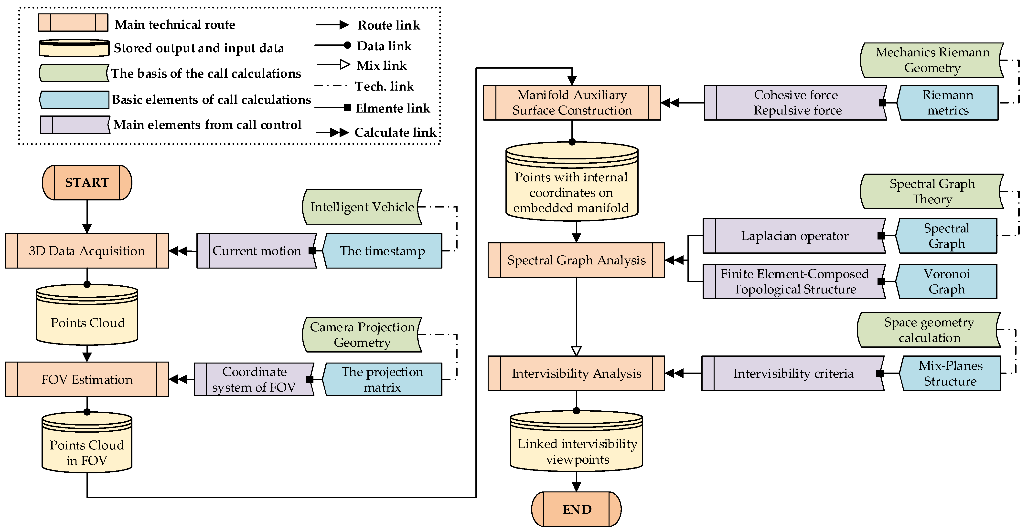
The remainder of this paper is organized as follows. Section 2 provides a streamlined, condensed, and key point-detailed introduction to the proposed method. Section 3 and Section 4 are the presentation and performance discussion of our results. Finally, Section 5 presents some concluding remarks. The roadmap of the method in this paper is shown in Figure 1.

2. Method

In this section, we have implemented our intervisibility analysis method through the progressive process of three subsections:

(1)

FOV estimation and point cloud generation at the current motion time of the intelligent vehicle;

(2)

Metrics construction of point cloud’s manifold auxiliary surface;

(3)

Spectral graph analysis of the finite element-composed topological structure on the manifold auxiliary surface, and the intervisibility analysis under the criterion based on the geometric calculation conditions of the mix-planes structure.

2.1. Estimation of Motion Field-of-View

The vehicle-mounted LiDAR acquires a 3D point cloud by reflecting the laser beams of surrounding objects and performing signal processing. The original LiDAR point cloud data is omni-directional; in its direct intervisibility analysis, there are complex calculations of redundant background points and noise points. For dynamic intervisibility analysis of autonomous driving scenes, we need to estimate the FOV of the intelligent vehicles at the current moment of motion.

Here we align the Lidar point cloud coordinate system, i.e., the Euclid-style 3D world coordinate system, with the dynamic camera coordinate system of the current motion to determine the FOV estimation of the current motion and obtain its corresponding point cloud sampling data. Among them, the result of the sampling points can be convolutional down-sampled with a spherical kernel of granularity $\tau$. This is because we do not need to calculate all points in subsequent operations. This convolutional down-sampling is the same as the traditional two-dimensional convolutional down-sampling method and the principle of the neural network (that is, the sample data are filtered with the convolution kernel in a sliding window, and each filtering produces a new local data result). However, the convolution kernel we used is an ordinary spherical kernel with a granularity $\tau$, the sample data is a 3D point cloud, and the sliding step length is the unit step length to the center of the nearest neighboring kernel.

The camera’s image can be used as a range guide for the current motion field of view. Therefore, we align the LiDAR point cloud coordinate system with the camera image plane coordinate system. First, the point cloud coordinate system to the camera coordinate system in the current state of motion is a rigid body motion matrix, i.e., it has undergone the transformation of rotation and translation. Then, the camera coordinate system to its image plane coordinate system is transformed by the mathematical model of camera projection, i.e., the internal reference matrix of the camera, which is a pre-calibrated camera parameter. Furthermore, there is a rotation transformation between the current state’s camera coordinate system and the initial state’s camera coordinate system. Finally, we obtain the motion FOV’s estimated point cloud result of the LiDAR’s omni-directional point cloud through this series of transformations. Then, the theoretical FOV calculation derived from the basic mathematical model of camera projection geometry and rigid body motion theory is completed with the following (1):

$$P_C^i=\left\{M^i{R}^0{M}_L^C\left(R,t\right)\right\}{P}_L^i$$

(1)

where $P_C^i$ is the point in the camera coordinate system of the angle of view at a time $i$th; $P_L^i$ is the point of 3D point cloud that is calibrated synchronously with the timestamp at the current time; $M^i$ is the projection matrix of the camera; $R^0$ is the rotation matrix of the camera coordinate systems in the initial state and current state;$M_L^C$ is the rigid body transformation matrix containing rotation $R$ and translation $t$ for LiDAR and camera coordinate systems. $M^i$ is calculated by geometric projection relations, as follows:

$$M^i=\left(\begin{array}{cccc}{F}^i& 0& x^i& -F^i{B}^i\\ 0& F^i& y^i& 0\\ 0& 0& 1& 0\end{array}\right)$$

(2)

where $(x^i,y^i)$, $F^i$, $B^i$ are the optical center, focal length, and baseline of the camera, respectively. In addition, to align the calculations of matrices in (1), the involved points use the homogeneous coordinate in the projection geometry to replace the Cartesian coordinate in the Euclidean geometry. Furthermore, the involved matrices are expanded by the Euclidean transformation matrix.

2.2. Manifold Auxiliary Surface for Intervisibility Computing

The space of the FOV estimated result of the LiDAR point cloud in the previous section is the Euclidean space. In a high-dimensional space such as the Euclidean space, the sample data is globally linear. That is, the sample data are independent and unrelated (e.g., the data storage structure of queues, stacks, and linked lists). However, the various attributes of the data are strongly correlated (e.g., the data storage structure of the tree). For the point cloud as sample data in this paper, the global distribution of its data structure in the high-dimensional space is not obviously curved, the curvature is small, and there is a one-to-one linear relationship between the points. However, in terms of the local point cloud and the x-y-z coordinate composition of the point itself, the distribution is obviously curved, the curvature is large, and there are too many variables affecting the point distribution. This is a kind of unstructured nonlinear data.

Furthermore, the direct intervisibility calculation for the point cloud is inaccurate because the point cloud in Euclidean space is globally linear, while the local points-to-points and the point itself are strongly nonlinear. Therefore, to reflect the global and local correlations between point clouds, Riemannian geometric relations in differential geometry, i.e., the geometry within the Riemannian space that degenerates to Euclidean space only at an infinitely small scale, are used to embed its smooth manifold mapping with Riemannian metric as an auxiliary surface for the intervisibility calculation.

The mathematical definition of the manifold is: Let $M$ denote a topological space, for any point $p$ on it belongs to $M$, there exists a homeomorphism open neighborhood $\Omega$ of $p$ with the open subset in the d-dimensional Euclidean space. Then $M$ is called a d-dimensional topological manifold, also called a d-dimensional manifold. The points on the manifold itself have no coordinates, thus to represent these data points, the manifold can be placed into the ambient space, and the coordinates on the ambient space can be used to represent the points on the manifold. For example, the spherical surface in the 3D space is a 2D surface. That is, the spherical surface has only two degrees of freedom, but we generally use the coordinates in the ambient space to represent this spherical surface.

For the natural coordinates of a point cloud with a three-dimensional observation dimension in the ambient space, a set of corresponding intrinsic coordinates are used to make the manifold on the low-dimensional plane as good as possible while maintaining the geometric characteristics and their metrics of the points. In order to have the intervisibility analysis of the point cloud that maintains the geometric characteristics, we use the Riemann metric to construct a manifold auxiliary surface as the mapping of the embedded manifold.

The Riemann metric is the metric of Riemann space. Roughly speaking, the Riemann metric is the radian between points in space. For example, considering the inertia matrix as a Riemann metric, the Lagrangian equation in mechanics can be expressed as a Riemannian manifold. The solution of the equation is the geodesic on the Riemannian manifold. The geodesic is defined as the shortest curve on the surface. The Riemann metric is the solution of the Lagrange equation in mechanics. This call is related to the geometrization of mechanics, that is, the short-range line between the point not subject to external forces and the real trajectory of the point in Riemannian space is the geodesic, as opposed to Euclidean space, which is a straight line. This metric is an expression of the kinetic energy introduced by the Lagrangian dynamical system. This paper uses cohesive forces and external repulsive forces of points to express these point-to-point metrics. The cohesive and repulsive forces are deduced based on the Artificial Potential Field theory of the forces potential field between the target and the obstacle (i.e., attractive and repulsive forces). We take the cohesive force between the dynamic viewpoint and the target point and the repulsion force with the initial meta-viewpoint to embody the Riemann metric between the points using the solution of the motion equations from fluid dynamics theory.

The cohesive force is the derivative of the cohesive field function with respect to the distance, as follows:

$$Cohesion:\left(P_C^i\right)=-\nabla F_{coh}\left({\displaystyle \sum P\left(P_C^i,P_C^i{}^{\ast }\right)}\right)=\alpha ·D\left(P_C^i,P_C^i{}^{\ast }\right)$$

(3)

where $F_{coh}\left({\displaystyle \sum P\left(P_C^i,P_C^i{}^{\ast }\right)}\right)$ is the cohesive field function ${\displaystyle \sum P\left(P_C^i,P_C^i{}^{\ast }\right)}=\left(\alpha ·D{\left(P_C^i,P_C^i{}^{\ast }\right)}^2\right)/2$; $\alpha$ is the cohesive scale factor; $D\left(P_C^i,P_C^i{}^{\ast }\right)$ indicates the cohesive forces of current data $P_C^i$ and target data $P_C^i{}^{\ast }$, and its specific performance is the Mahalanobis distance after the original Euclidean distance between the viewpoints has been rotated and scaled, as follows:

$$D\left(P_C^i,P_C^i{}^{\ast }\right)=\sqrt{{\left(P_C^i(X)-P_C^i{}^{\ast }(Y)\right)}^T{\sum }^{-1}\left(P_C^i(X)-P_C^i{}^{\ast }(Y)\right)}$$

(4)

where ${\sum }^{-1}$ is the covariance matrix $\mathrm{cov}(X,Y)={\displaystyle {\sum }_{i=1}^n(X_i-\overline{X})}(Y_i-\overline{Y})/(n-1)$. In the matrix calculation process in (4), there will be cases where the samples are independent and identically distributed, i.e., the covariance matrix is a diagonal matrix that is not full of rank, so it degenerates into a normalized Euclidean distance, as follows:

$$D\left(P_C^i,P_C^i{}^{\ast }\right)=\sqrt{{\displaystyle {\sum }_{i=1}^n\frac{{\left(X_i-Y_i\right)}^2}{{\sigma }_i^2}}}$$

(5)

where ${\sigma }_i^2$ is the standard deviation.

The external repulsive force is the gradient of the repulsive function, as follows:

$$\begin{array}{l}Repulsion:(P_C^i)=-\nabla F_{rep}\left({\displaystyle \sum P\left(P_C^i{}^0,P_C^i\right)}\right)\\ =\{\begin{array}{c}\beta \left(\frac{1}{D^{\prime }\left(P_C^i{}^0,P_C^i\right)}-\frac{1}{Radius(·)}\right)=\frac{1}{D^{\prime }{\left(P_C^i{}^0,P_C^i\right)}^2}\nabla D^{\prime }\left(P_C^i{}^0,P_C^i\right),\begin{array}{c}\end{array}{D}^{\prime }\left(P_C^i{}^0,P_C^i\right)\le Radius(·)\\ 0,\begin{array}{ccc}\begin{array}{ccc}\begin{array}{cc}\begin{array}{ccc}& & \end{array}& \end{array}& & \end{array}& & \end{array}{D}^{\prime }\left(P_C^i{}^0,P_C^i\right)>Radius(·)\end{array}\end{array}$$

(6)

where $Radius(·)$ is the influence radius of the point $P_C^i$ on surrounding points (i.e., the further the distance from the data point $P_C^i{}^0$, the more the repulsion is negligible to 0); $F_{rep}\left({\displaystyle \sum P\left(P_C^i{}^0,P_C^i\right)}\right)$ is the repulsive field function:

$${\displaystyle \sum P\left(P_C^i,P_C^i{}^{\ast }\right)}=\{\begin{array}{cc}\frac{1}{2}\beta {(\frac{1}{D^{\prime }\left(P_C^i{}^0,P_C^i\right)}-\frac{1}{Radius(·)})}^2& ,D^{\prime }\left(P_C^i{}^0,P_C^i\right)\le Radius(·)\\ 0& ,D^{\prime }\left(P_C^i{}^0,P_C^i\right)>Radius(·)\end{array}$$

(7)

where $\beta$ is the repulsive scale factor; $D^{\prime }\left(P_C^i{}^0,P_C^i\right)$ indicates the repulsive forces of current data $P_C^i$ and initial meta-viewpoint data $P_C^i{}^0$, and its specific performance is the shortest path distance of the flow path that satisfies the derived Formula (8) of hydrodynamics of gravitational breadth-first. Formula (8) shows continuity differential equations (underlying the law of conservation of mass): Euler’s equations of motion (underlying Newton’s Second Law of Motion-Force and Acceleration), and Bernoulli’s equations (underlying the stable flow of ideal fluid). In this paper, we use the simple weighted sum of the shortest distance for the points as the shortest path. In particular, this point-to-point distance calculation is consistent with the involved distance in the above cohesive force, i.e., they both use Mahalanobis distance to ensure the unit is scale-independent.

$$\{\begin{array}{l}\partial k/\partial s+\nabla ·k·\overrightarrow{v}=0\\ d\overrightarrow{v}/ds-\overrightarrow{f}+grad\left(P_C^i{}^0\right)/k=0\\ \overrightarrow{v}·d\overrightarrow{v}+d\left(P_C^i{}^0\right)/k+grad\left(P_C^i{}^0\right)·dz=0\end{array}$$

(8)

where $k$ is the density of data points in the flow process, i.e., the number; $s$ is the flow time, i.e., the step length; $\overrightarrow{v}$ is the flow velocity, i.e., the flow distance of components in $x,y,z$ directions; $\partial$ is the expansion operation according to Taylor series; $grad(P_C^i{}^0)$ is the gradient, i.e., $\partial P_C^i{}^0/\partial x+\partial P_C^i{}^0/\partial y+\partial P_C^i{}^0/\partial z$; $d\overrightarrow{v}/ds$ is the partial derivative of the flow time of the velocity in each flow direction component of $x,y,z$; $\overrightarrow{f}$ is the unit distance of the flow in the directions of $x,y,z$.

In doing so, we make the manifold structure embedded in the point cloud in the FOV scale-independent. This structure can be computed independently of the measurement scale and considers the sparsity property link between the intervisibility data (current point $P_C^i$, meta-viewpoint $P_C^i{}^0$, surrounding passable intervisibility points $P_C^i{}^{\ast }$). This contribution is mainly because our metric is a metric in Riemannian geometry. The specific force performance is to use Mahalanobis distance instead of Euclidean distance. The difference between Mahalanobis distance and Euclidean distance is that it is independent of the measurement scale and considers the relationship between various features. Because in the process of calculating the distance, the components of the two points will be normalized first (that is, rotating the coordinate axis, performing the corresponding linear transformation, so that the variables remove the units), and then the distance is calculated. In this way, the transformed components are linearly independent, and the difference between the two points can be better reflected than the Euclidean distance. Therefore, the manifold structure embedded in the point cloud in the FOV can be scale-independent.

2.3. Spectral Graph Analysis of Finite Element-Composed Topological Structure

We use points $P(P_C^i{}^{\prime },\dots P_C^{i*}{}^{\prime })$ on the above-mentioned auxiliary surface to construct the finite element mesh of the Voronoi graph $G(Nodes(P_C^i{}^{\prime }),Edges(\overrightarrow{P_C^i{}^{\prime },P_C^i{{}^{\ast }}^{\prime }}))$(i.e., $G\left(P,E\right)$) based on the principle of an empty circle that any four points cannot be co-circular and the principle of maximizing the minimum angle according to the enlighten mode of point-by-point insertion of the Bowyer–Watson algorithm. We further calculate the spectral graph analysis of the graph $G$, i.e., the Laplacian operator containing nodes points, adjacent edges, edges weights, and points degrees (degree matrix-composed and adjacency matrix-composed Laplacian matrix of the grid points), as follows:

$$L:={\displaystyle {\sum }_{N\times N}{P}_C^i{{}^{\prime }}_{(r,c)}}=D-A={\displaystyle {\sum }_{c=1}^N{w}_{(r,c)}-}{\displaystyle {\sum }_{c:\{r,c\}\in edges}\left(P_C^i{}^{\prime },P_C^{i*}{}^{\prime }\right)}$$

(9)

where $D$ is the degree matrix; $A$ is the adjacency matrix; $r,c$ are rows and columns of the matrix; $w_{(r,c)}$ is the weighted degree of nodes $P_C^i{}^{\prime }$.

The above Laplacian matrix can be normalized to $1_N·L=\left({\left(1,1,\dots ,1\right)}^T/\sqrt{N}\right)·L$, then, $L$ is:

$$\mathcal{L}:=D^{-1/2}·L·D^{-1/2}=D^{-1/2}·(D-A)·D^{-1/2}=I-\mathcal{A}$$

(10)

where $I$ is the unit matrix; $\mathcal{A}$ is the regularized adjacency matrix $\mathcal{A}=D^{-1/2}·A·D^{-1/2}$.

We prove that all points $P\left(P_C^i{}^{\prime },\dots P_C^{i*}{}^{\prime }\right)$ satisfy the following distance-based measure (10) through the above-mentioned Laplacian matrix of spectral analysis,

$$\begin{array}{l}P{\left(P_C^i{}^{\prime },\dots P_C^{i*}{}^{\prime }\right)}^T·L·P\left(P_C^i{}^{\prime },\dots P_C^{i*}{}^{\prime }\right)=P^T·D·P-P^T·A·P\\ ={\displaystyle \sum _{c=1}^N{\displaystyle {\sum }_{c=1}^N{w}_{(r,c)}}·}{P}^2-{\displaystyle \sum _{r,c=1}^N{w}_{(r,c)}·P_r·P_c}\\ =\frac{1}{2}\left({\displaystyle \sum _{c=1}^N{\displaystyle {\sum }_{c=1}^N{w}_{(r,c)}}·}{P}_c{}^2-2{\displaystyle \sum _{r,c=1}^N{w}_{(r,c)}·P_r·P_c}+{\displaystyle \sum _{r=1}^N{\displaystyle {\sum }_{r=1}^N{w}_{(r,c)}}·}{P}_r{}^2\right)\\ =\frac{1}{2}{\displaystyle \sum _{r,c=1}^N{w}_{(r,c)}{\left(P_c-P_r\right)}^2}\end{array}$$

(11)

The above (11) corresponds to the sum of distances of multiple data points when $w_{(r,c)}=1$.

We perform a spectral decomposition $SD\left(P\left(P_C^i{}^{\prime },\dots P_C^{i*}{}^{\prime }\right)\right)$ based on the above distance measure. The point determination is divided into intervisibility points and non-intervisibility points.

$$SD\left(P\left(P_C^i{}^{\prime },\dots P_C^{i*}{}^{\prime }\right)\right):={\displaystyle {\sum }_{c=1}^{N}A\left({\displaystyle \sum P_C^i{}^{\prime }},{\displaystyle \sum {\widehat{P}}_C^i{}^{\prime }}\right)}/2$$

(12)

where ${\displaystyle \sum {\widehat{P}}_C^i{}^{\prime }}$ is the set of intervisibility points, ${\displaystyle \sum P_C^i{}^{\prime }}$ is the set of residual points, i.e., non-intervisibility points; $A\left(P_C^i{}^{\prime },{\widehat{P}}_C^i{}^{\prime }\right)$ can be calculated as ${\displaystyle {\sum }_{c:\{r,c\}\in edges}^N{w}_{(r,c)}}\left(P_C^i{}^{\prime },P_C^{i*}{}^{\prime }\right)$, here, $P_C^{i*}{}^{\prime }$ is all the neighboring adjacent points of $P_C^i{}^{\prime }$.

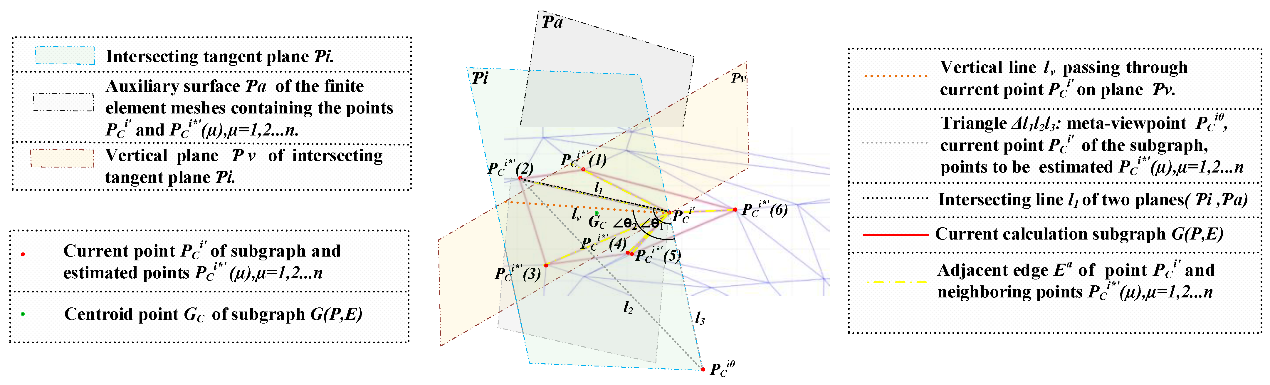
We construct the Mix-Planes Calculation Structure (MPCS) shown in Figure 2 for the current point $P_C^i{}^{\prime }$. The dihedral angle $\angle {\theta }_2$ of plane ${\mathcal{P}}_i$ and plane ${\mathcal{P}}_v$ is a straight dihedral angle, i.e., ${\theta }_2=90\mathrm{deg}$. The angle $\angle {\theta }_1$ between intersection lines $l_1$ and $l_3$ of planes ${\mathcal{P}}_i$ and ${\mathcal{P}}_a$ is calculated by the inner product $dot(·)$ and module $norm{(·)}_2$ of the intersection angle’s arccosine $acosd(·)$ for three-point vectors $P^{\mathcal{C}}$ and $P^{\mathcal{E}}$, as follows:

$$\{\begin{array}{l}{\theta }_1=acosd\left\{dot\left(\left(P^{\mathcal{C}}\right),\left(P^{\mathcal{E}}\right)\right)/\left(norm{\Vert P^{\mathcal{C}}\Vert }_2\ast norm{\Vert P^{\mathcal{E}}\Vert }_2\right)\right\}\\ P^{\mathcal{C}}=\overrightarrow{\left(P_C^{i0},P_C^i{}^{\prime }\right)};P^{\mathcal{E}}=\overrightarrow{\left(P_C^{i\ast }{}^{\prime }\left(\mu \right),P_C^i{}^{\prime }\right)}\end{array}$$

(13)

where the range of ${\theta }_1$ is $\left[0\mathrm{deg},180\mathrm{deg}\right]$.

We use the Laplacian matrix of the spectral graph analysis to decompose the satisfied objective function $SD(·)$ to obtain the intervisibility points that meet the intervisibility criteria. The criteria are composed of geometric calculation conditions in the above calculation structure MPCS, The Algorithm 1 of determination process is as follows:

Algorithm 1 The criteria determination process of reachable intervisibility points
1:	for ${\displaystyle {\sum }_{\{r,c\}=1\in L}^{N\times N}{P}_C^i{}^{\prime }}$ of $\forall G\left(P,E\right)$ and $D(l_1)<D_{\min }<D^{\prime }(l_3)$ do
2:	if     $\exists D\left(l_1\right)<D\left(l_{gc}\right)$ for $\forall G\left(P,E\right)$ then
3:	update $P_C^i{}^{\prime }=P_C^{i*}{}^{\prime }$ for $D\left(P_C^i{}^{\prime },P_C^{i*}{}^{\prime }\right)=D_{\min }$;
4:	end if
5:	else if $D\left(l_1\right)>D\left(l_{gc}\right)$ then
6:	find ${\widehat{P}}_C^{i*}{}^{\prime }$ for $\left(\theta 1-\theta 2\right)>0 \&\&\left(Z\left(P_C^{i*}{}^{\prime }\right)-Z\left(P_C^i{}^{\prime }\right)\right)>0$;
7:	update $G\left(P,E\right)$ of $P\left({\widehat{P}}_C^i{}^{\prime },{\widehat{P}}_C^{i*}{}^{\prime }\right)$ and $E\left({\widehat{P}}_C^i{}^{\prime },{\widehat{P}}_C^{i*}{}^{\prime }\right)$;
8:	find ${\widehat{P}}_C^{i*}{}^{\prime }$ for $\left(\theta 1-\theta 2\right)<0 \&\&\left(Z\left(P_C^{i*}{}^{\prime }\right)-Z\left(P_C^i{}^{\prime }\right)\right)<0$;
9:	update $G\left(P,E\right)$ of $P\left({\widehat{P}}_C^i{}^{\prime },{\widehat{P}}_C^{i*}{}^{\prime }\right)$ and $E\left({\widehat{P}}_C^i{}^{\prime },{\widehat{P}}_C^{i*}{}^{\prime }\right)$;
10:	end if
11:	end for
12:	return $P_C^i{}^{\prime }$

where $D\left(l_1\right)=D{\left(P_C^i{}^{\prime },P_C^{i*}{}^{\prime }\right)}_{\mu },\mu =1,2\dots n\in G\left(P,E\right)$; $D_{\min }$ is the minimum degree of the adjacency matrix of the subgraph, i.e., the shortest radius distance threshold of the graph;$D^{\prime }\left(l_3\right)=D^{\prime }\left(P_C^i{}^0,P_C^{i^{\prime }}\right)$; $D\left(l_{gc}\right)=D\left(P_C^i{}^{\prime },G_c\right)$;$Z(·)$ is the elevation values of points; $G_c$ is obtained by the three-point area formula of all finite element meshes composed of the subgraph, and the calculation can be proved by the dovetail theorem, as follows:

$$G_c\left(x_c,y_c\right)=\{\begin{array}{l}{x}_c={\displaystyle {\sum }_{k=1}^n{x}_k{\mathcal{S}}_k}/{\displaystyle {\sum }_{k=1}^n{\mathcal{S}}_k}\\ y_c={\displaystyle {\sum }_{k=1}^n{y}_k{\mathcal{S}}_k}/{\displaystyle {\sum }_{k=1}^n{\mathcal{S}}_k}\end{array}$$

(14)

where ${\mathcal{S}}_k,k=1,2,\dots n$ is the area of all finite element meshes in the subgraph, e.g., for one finite element mesh $\Delta k^{th}\left(x_{1,2,3},y_{1,2,3}\right)$, ${\mathcal{S}}_k=\left\{\left(x_2^k-x_1^k\right)\ast \left(y_3^k-y_1^k\right)-\left(x_3^k-x_1^k\right)\ast \left(y_2^k-y_1^k\right)\right\}/2$.

The physical meaning of the aforementioned criteria is actually to judge the upward and downward concave–convex characteristics of the spectral subgraph, i.e., whether the current point $P_C^i{}^{\prime }$ is inside the subgraph or outside the subgraph, and to judge whether the elevation values of adjacent points $P_C^{i*}{}^{\prime }$ are visible according to the geometry calculation. Under the premise of controlling the smoothness of the Laplacian matrix, step 1 controls whether the weighted value of the weighted Laplacian matrix corresponding to the calculation point and adjacent points is too large compared to the visible area radius of the line-of-sight. Once it is too large, this subgraph likely contains connected viewpoints in the space of the background environment far away from each other. Steps 2 and 4 control the spatial position of the current operating point in this subgraph, i.e., remove the spectral calculation composed of inhomogeneous finite elements so that it will not operate at the concave boundary. The advantage of this is to preserve the cohesive targets in the scene as much as possible. Steps 5 and 7 determine the intervisibility of the finite element mesh by the concave–convex centripetal properties of the subgraph composed of the current operating point (i.e., the dispersion) and the elevation values of neighboring nodes. The centripetal heart here is the meta-viewpoint. The more discrete the current operation point and the meta-viewpoint are, the more the concave–convex centrality of the subgraph deviates, and the more the finite element mesh will bulge farther.

At this point, we have obtained the final tree-like linked structure of the finite element-composed topological structure, including intervisibility points and reachable edges, i.e., $G\left(Nodes\left({\widehat{P}}_C^i{}^{\prime }\right),Edges\overrightarrow{\left({\widehat{P}}_C^i{}^{\prime },{\widehat{P}}_C^i{{}^{\ast }}^{\prime }\right)}\right)$. All finite elements are defined as the intervisible region that contains the finite element mesh when the finite element have intervisible three-points and two more intervisible edges of adjacent points. This benefits from the fact that two points can only determine the reachability of a line, while three points that are not collinear can determine a surface is a theorem.

3. Results

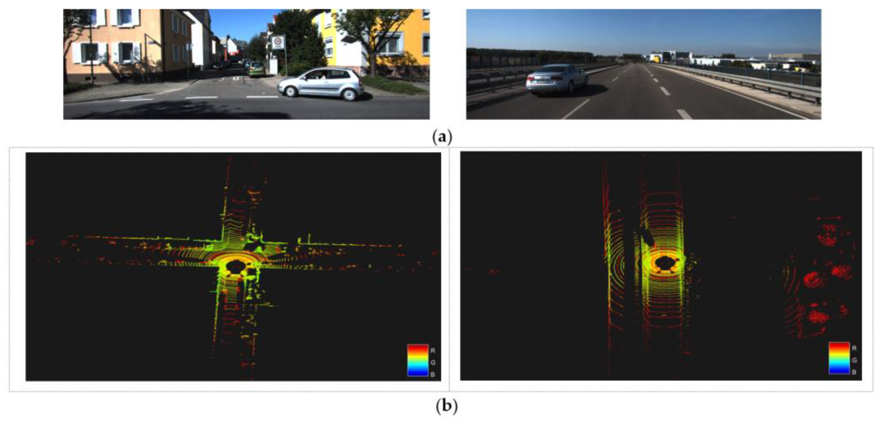
We conducted experiments on dynamic intervisibility analysis of 3D point clouds in benchmark KITTI, the most well-known and challenging dataset for autonomous driving on urban traffic roads. Here, we show the results and experiments for two scenarios. Scenario one is an inner-city road scene, and scenario two is an outer-city road scene. In addition, the equipment, platform, and environment configuration involved in our experimental environment are shown in

Table 1. Experimental environments.

Experimental Environments
Equipment	Camera: 1.4 Megapixels: Point Grey Flea 2 (FL2-14S3C-C) LiDAR: Velodyne HDL-64E rotating 3D laser scanner, 10 Hz, 64 beams, 0.09-degree angular resolution, 2 cm distance accuracy
Platform	Visual studio 2016, Matlab 2016a, OpenCV 3.0, PCL1.8.0
Environment	Ubuntu 16.04/Windows 10, Intel(R) Core(TM) i7-8750H CPU @ 2.20GHz, NVIDIA GeForce GTX 1060/Intel(R) UHD Graphics 630

.

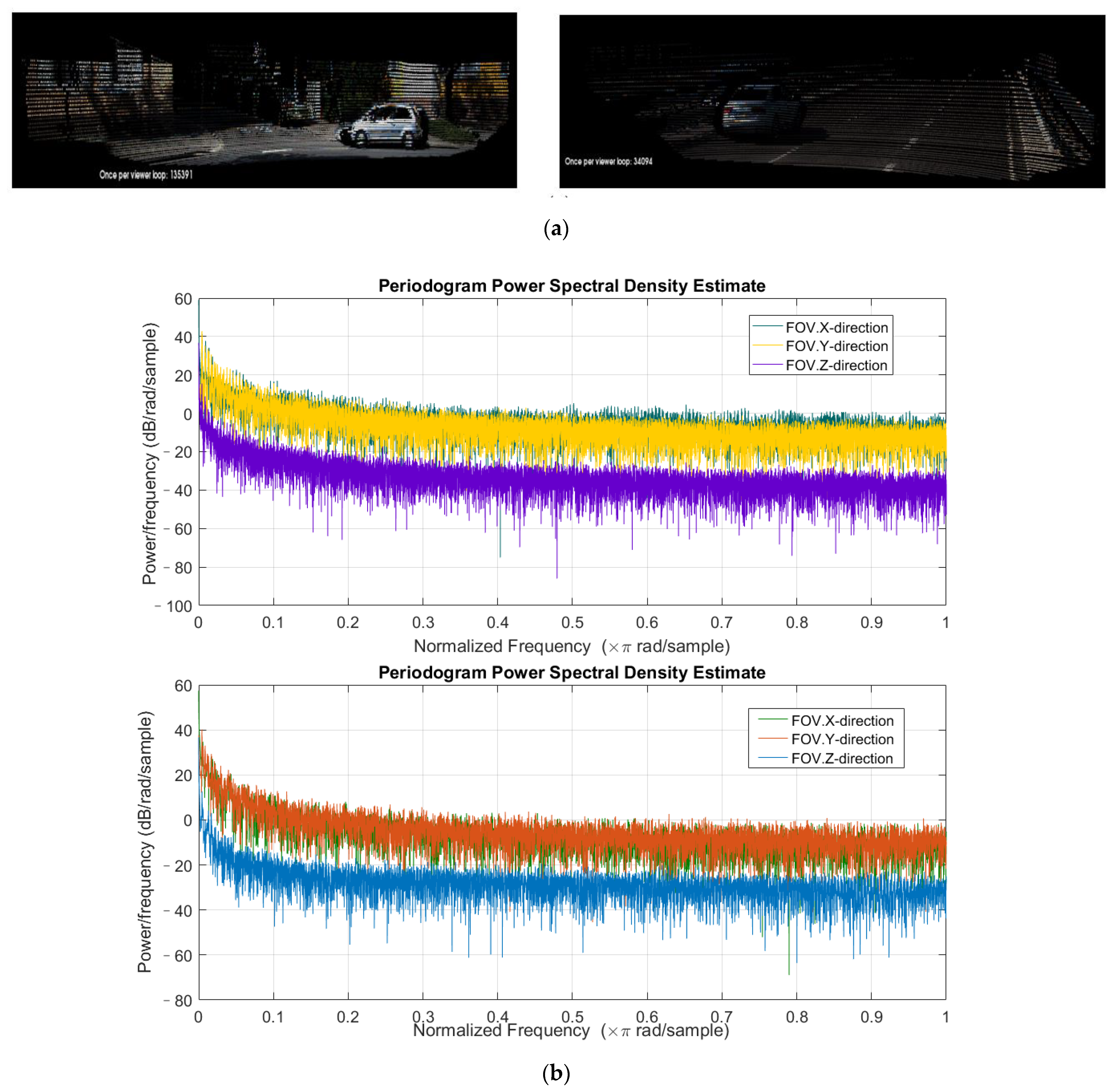
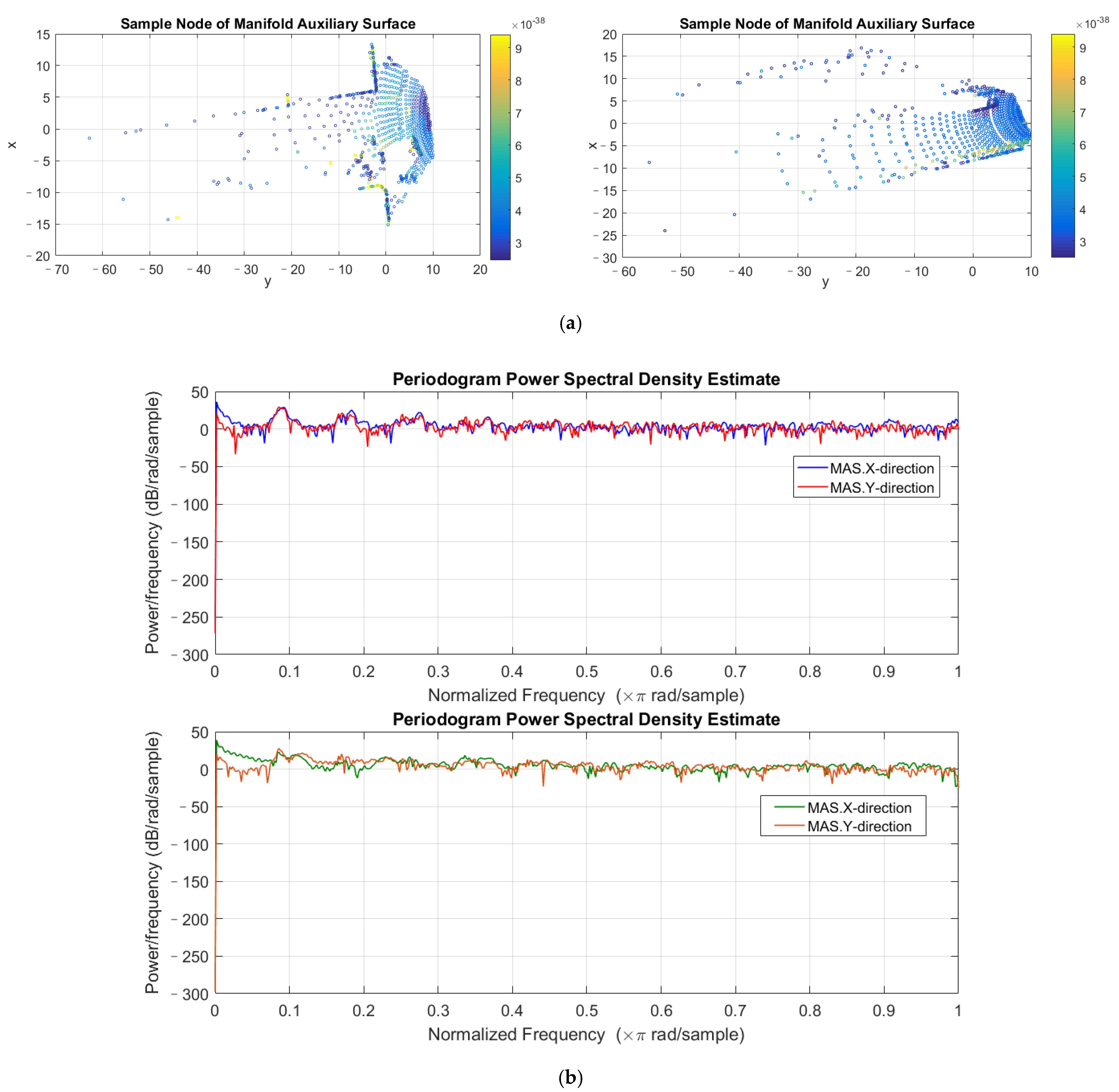
Figure 3 shows the image of the FOV and the corresponding top view of the LiDAR 3D point cloud acquired by the vehicle in a moment of motion. The color of the point cloud represented the echo intensity of the Lidar. Figure 4a presents the point cloud sampling results for the FOV estimation of the current motion scene after we aligned the multi-dimensional coordinate systems. We effectively removed the invisible point cloud outside the field of view, especially the outlier background points. Figure 4b then shows the power spectra of the resultant signals in different directions. Their frequency resolution is high, but the spectral peaks are difficult to determine.

Figure 5a shows the point mapping of our Manifold Auxiliary Surface (MAS) for the original point cloud data, while Figure 5b shows the signal power spectrum of the MAS. The colorbar represents the different labels of the points, and the color texture labels of the 3D point cloud were used here. Although there were drastic abrupt changes caused by discrete background points, the overall power spectrum density was smooth with better noise suppression and fewer chaotic characteristics compared to the point cloud power spectrum of the estimated FOV when a certain frequency resolution was ensured.

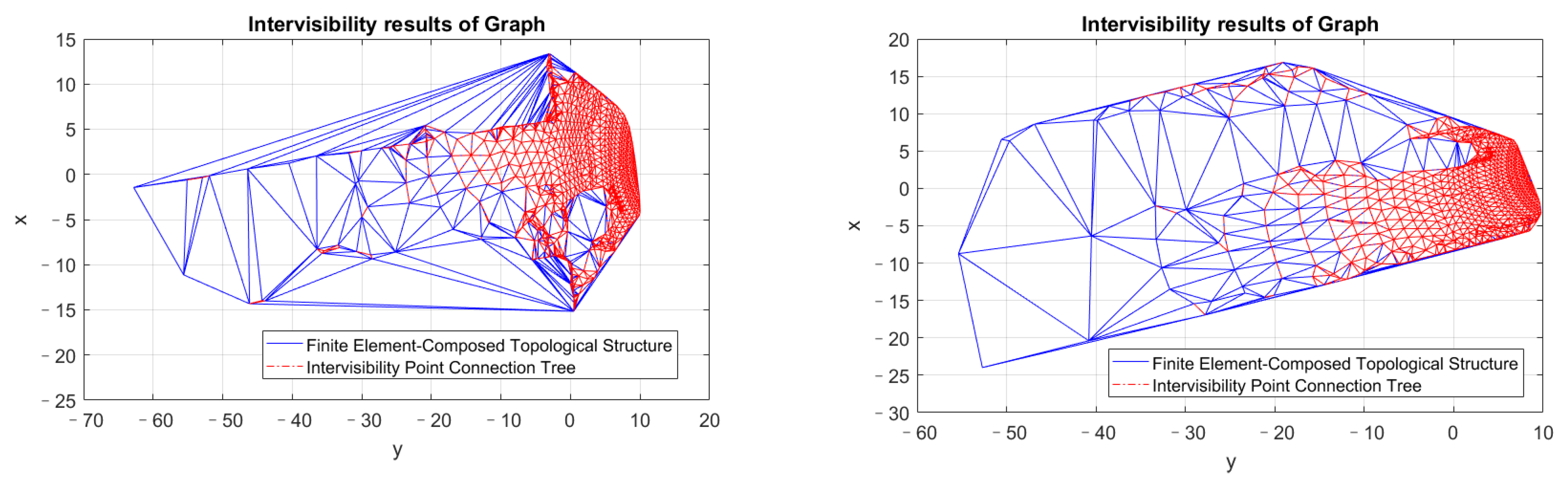
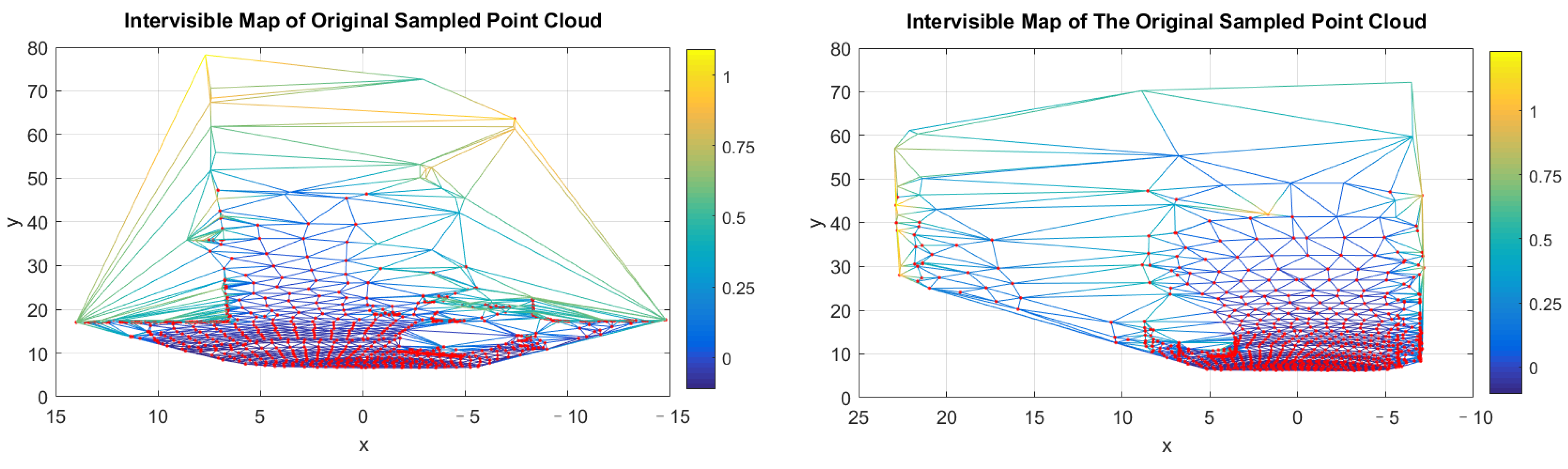
From the constructed finite element topology structure of the MAS and the linked intervisibility points and edges of the spectral graph analysis results in Figure 6, we effectively screened out the irrelevant invalid edges linked to the background and unconnected invisible points in the graph. The irrelevant invalid edges linked to the background and unconnected invisible points are removed directly. Visible viewpoints on this tree’s local lines of depth and width traversal nodes were also linked as isolated edges. Although it was also effective for intervisibility, these separate appearances were not very meaningful for the dynamic intervisibility analysis of autonomous driving. Therefore, they could be ignored to some extent. We visualized the intervisibility points on the original FOV estimation result in Figure 7. The colors of the edges of all points corresponded to their different elevation distance weights, and the red points were the locations of the intervisibility points.

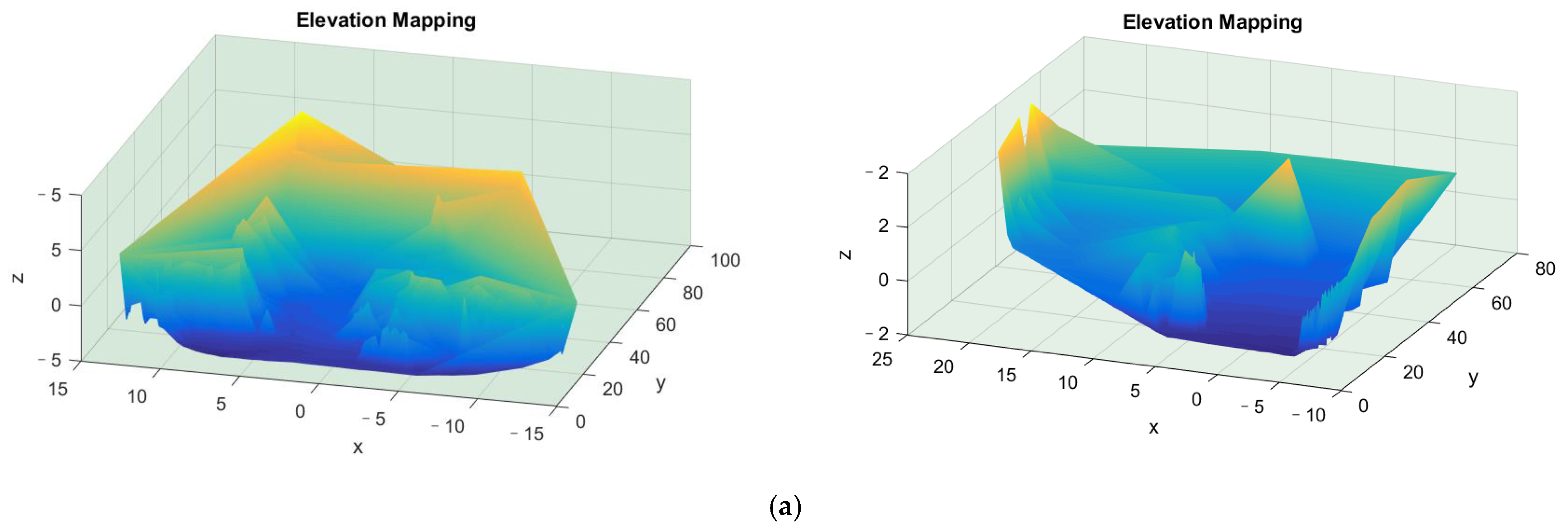
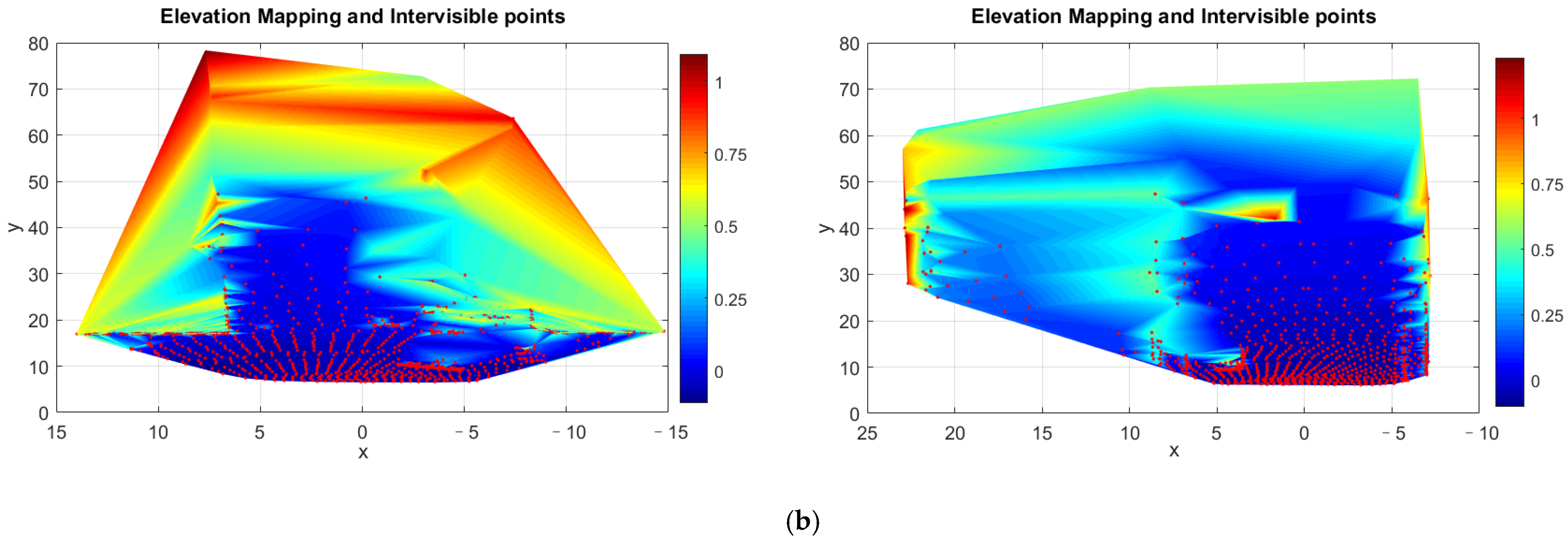
The final evaluation mapping of the 3D intervisibility terrain area of the vehicle driving within the current FOV is shown in Figure 8. In order to further visually display the three-dimensional visual effects of the result of the intervisibility point and the terrain elevation value, the map was based on the FOV coordinate structure in Figure 7 for the terrain mapping, and the elevation value mapping and the corresponding element grid surface shading were added. We showed the area where the vehicle can be guided driving and the mapping of the red intervisibility point, where the colorbar corresponded to the size of the elevation value, and the red points were the mappings of the intervisibility points.

4. Results Analysis and Discussion

In order to discuss the results of the intervisibility effectively and clearly, we used the following metrics to evaluate the results of the experiments. N is the number of finite element meshes of the composite topological structure of points on the manifold auxiliary plane. SP is the number of adjacent decision points in the subgraph. The greater the number, the greater the calculation levels and the greater the amount of calculation.

Average node Redundancy Removal rate (ARR):

$$ARR={\displaystyle \sum \left(P_L^i-P_C^i{}^{\prime }\right)/P_L^i}\times 100$$

(15)

The higher the ARR, the more redundant nodes are removed. The more effective the method is.

Two-Point Intervisibility rate (TPI):

$$TPI=\frac{1}{3N}{\displaystyle \sum \overrightarrow{\left({\widehat{P}}_C^i{}^{\prime },{\widehat{P}}_C^i{{}^{\ast }}^{\prime }\right)}}\times 100$$

(16)

The closer the TPI is to the global point method, the closer the result is to the real intervisibility. It reflects the intervisibility of 3D point clouds. TPI is the proportion of all edges of the finite element that do not exclude repeatedly connected edges. It represents the two-way interoperability in a directed graph of two points. The actual exclusion of adjacent edges of neighboring finite elements has a higher TPI.

Decreasing Calculation Quantity rate (DCP):

$$DCP=\left({\displaystyle \sum \overrightarrow{\left(P_L^i,P_L^i{}^{\prime }\right)}}-{\displaystyle \sum \overrightarrow{\left(P_C^i{}^{\prime },P_C^i{{}^{\ast }}^{\prime }\right)}}\right)/{\displaystyle \sum \overrightarrow{\left(P_L^i,P_L^i{}^{\prime }\right)}}\times 100$$

(17)

The higher the DCP, the shorter the calculation time and the higher the efficiency of the method.

The metrics of results for samplings of different particle sizes are shown in

Table 2. The intervisibility results for different 3D point clouds.

Samplings	N	SP	ARR (%)	TPI (%)	DCP (%)
10	3982	5982	98.40	47.61	95.46
20	1984	2984	99.20	44.17	97.90
30	1320	1986	99.47	41.04	98.70
40	987	1487	99.60	38.57	99.09
50	786	1186	99.68	35.79	99.33
60	653	986	99.73	35.78	99.44
70	557	842	99.77	33.87	99.55
80	488	738	99.80	30.94	99.64
90	432	654	99.82	31.33	99.68
100	388	588	99.84	30.50	99.72

. The particle size is the granularity of the spherical kernel mentioned in Section 2.1.

Table 3. The different run indicators of different 3D point cloud samplings.

Samplings	S1 (s)	S2 (s)	S3 (s)	TIME (s)	AS1 (s)	AS2 (s)	AS3 (s)	ATIME (s)	VAR (%)	STD (%)
10	0.0010	0.0053	0.3854	0.3917	0.00083	0.00515	0.36934	0.37532	0.9197	0.9695
20	0.0008	0.0026	0.1696	0.1730	0.00080	0.00281	0.16817	0.17178	0.5848	0.6165
30	0.0008	0.0018	0.1105	0.1131	0.00076	0.00183	0.11383	0.11642	0.2544	0.2682
40	0.0008	0.0015	0.0858	0.0881	0.00075	0.00150	0.08842	0.09067	0.1532	0.1615
50	0.0008	0.0013	0.0808	0.0829	0.00074	0.00157	0.08625	0.08856	0.2615	0.2757
60	0.0009	0.0011	0.0619	0.0639	0.00078	0.00116	0.06341	0.06535	0.1819	0.1918
70	0.0007	0.0011	0.0651	0.0669	0.00079	0.00107	0.06327	0.06513	0.4069	0.4289
80	0.0009	0.0010	0.0592	0.0611	0.00075	0.00091	0.05188	0.05354	0.1563	0.1648
90	0.0009	0.0009	0.0521	0.0539	0.00072	0.00093	0.05130	0.05295	0.1732	0.1825
100	0.0008	0.0008	0.0459	0.0475	0.00073	0.00088	0.04672	0.04833	0.2473	0.2607

shows the one run and 10 runs average running time of the proposed in this paper. S1 is the calculation time of the MAS, S2 is the construction time of the finite element topological structure, and S3 is the time for the spectral analysis to calculate the intervisibility point. TIME is the calculation time of the intervisibility point of this paper. A-X (AS1, AS2, AS3, ATIME) are the average measurements of the 10 runs of the samplings. VAR is the variance of TIME, and STD is the standard deviation of TIME, reflecting the degree of dispersion between the computational complexity of each run and the average computational complexity. The smaller the VAR and STD values, the smaller the dispersion’s degree, reflecting the higher stability and stronger robustness of our method. We can see from the two tables that our calculation effectiveness and efficiency in this paper are both high.

Table 4. The metrics of different intervisibility analysis methods.

Methods	Nodes	ARR (%)	TPI (%)	DCP (%)	TIME (s)
Global Points	12,5148	-	50.72	-	1163.876
Interpolation Points	20,008	84.01	50.01	52.08	17.537
OURS	572	99.54	50.25	98.65	0.1044

shows the evaluation metrics of different intervisibility analysis methods. Among them, the method of judging the global point elevation value does not take relevant processing to reduce the amount of calculation, so there are no values of ARR and DCP, which can be regarded as 0. Experiments were carried out in the same test environment and based on the same original LiDAR data. Among them, the global point method and the interpolation point method simply removed the background noise points. The final number of nodes used to represent the terrain visibility calculation is the smallest in our method. This removal will be required for the premise of ensuring a certain information rate to avoid too few nodes in the future. Compared with the intervisibility analysis methods of global points and interpolation points, our dynamic intervisibility analysis of 3D point clouds maintain a significant and equivalent two-point intervisibility rate while the removal rate of redundant nodes and the decrement calculation amount are as high as 99.54% and 98.65%, respectively. Furthermore, our computation time can reach an average processing time of 0.1044 s for one frame with a 25 fps acquisition rate of the original vision sensor, which meets the reliability of online dynamic intervisibility analysis. In addition, the results of our intervisibility analysis between consecutive frames are stable and robust.

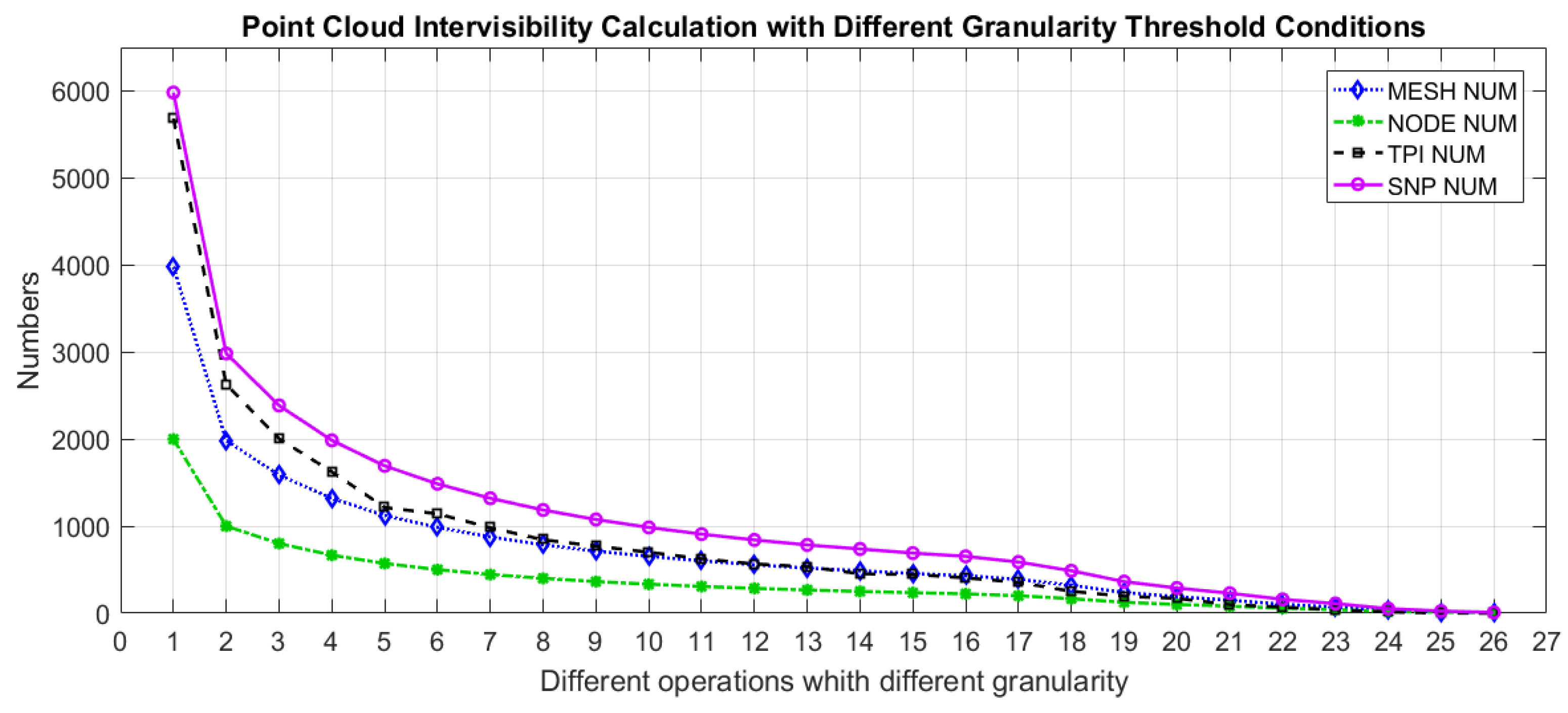
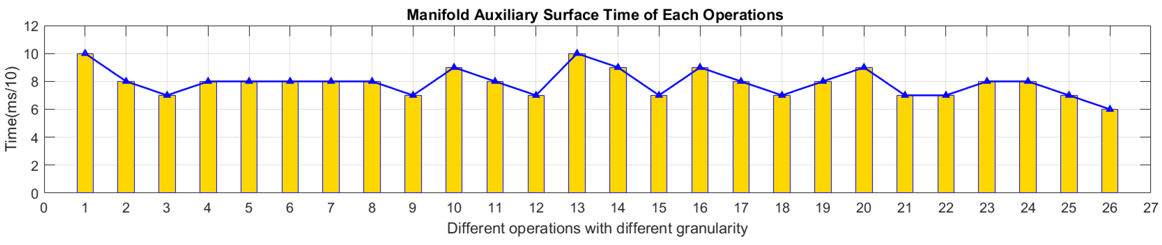
Figure 9 is a comparison of our intervisibility calculations under different granularity thresholds. Figure 10 is the calculation time of the MAS for different samplings with different granularity sizes. We can see that as the granularity increases, several quantities involved in the intervisibility calculation process for different samplings tend to move downward and gradually become smoother. There is a clear downward trend between 1–10, and after 10, or even after 20, it is basically smooth. Furthermore, their running time variance is 0.9061, the standard deviation is 0.9519, the degree of dispersion is low, and the robustness is strong. Therefore, the granularity threshold can be dynamically and automatically selected based on the current sampling.

Compared with the global point cloud and the local interpolation point clouds pathway-based method, our method does not directly process the original point cloud data. Our method effectively filters out excessive redundant noise 3D points. However, the deletion of too many points will undoubtedly affect the integrity of the information. For example, it can lead to the lack of information about essential targets in the scene and terrain. Among the different node numbers calculated by different methods based on the same original data, we had fewer data points, but we guaranteed the same quality of the two-point intervisibility rate to a certain extent.

Furthermore, to avoid the impact of information scarcity, it is indeed necessary to set and explore the minimum suppression threshold of the nodes number for automatic and dynamic collection requirements in future research. Moreover, the estimation of FOV is consistent with the actual motion scene of autonomous driving. The FOV estimation was necessary for dynamic analysis of autonomous driving scenarios because the original lidar data was omni-directional, and the motion view of intelligent vehicles changed at any time. In addition, our FOV results are equivalent to partial data based on the original data. Therefore, the length of the sampled signal is less than the length of the omni-directional data. Under the same sampling frequency, the frequency resolution of the FOV result is not higher than the original data. However, although the frequency resolution of the original data is sufficiently high, the accompanying data volume is substantial, the noise points are massive, the calculation time is long, and the cost is high. Therefore, the high frequency resolution of the original massive data is also a pity for dynamic intervisibility analysis. Such a balance is difficult to guarantee, and we can only take measures to maintain online in real-time. This is also an issue worthy of further research and innovation.

The construction of the MAS of the point cloud aligned with multi-dimensional data on the basis of Riemannian geometric manifold learning cannot only be limited to the transformation between three-dimensional and two-dimensional space. It can also expand the transformation from multi-dimensional space to low-dimensional space containing contextual semantic information. Finally, the proposed intervisibility analysis based on the spectral graph theory provides a basis for the analysis of the current motion space environment of autonomous driving. The analysis has risen from the low-level point-level features of the points to the spatial and geometric characteristics, which is efficient and robust. This paper has a certain guiding significance for subsequent automatic control, path planning, and Simultaneous Localization And Mapping (SLAM). In the future, continuous scene composition and point cloud splicing based on dynamic visibility analysis of current motion scenes in this paper will be our research focus.

5. Conclusions

The dynamic intervisibility analysis of 3D point clouds proposed in our paper avoids the errors of Euclidean calculation in space and the redundant calculations of traditional global points and interpolation points in efficiency. Our calculations are not limited to point-level operations. It effectively distinguishes the background and the target and makes the points of intervisibility more cohesive. The subgraph spectral decomposition of the mix-planes calculation structure under Riemann geometry for intervisibility analysis has obtained significant and influential visualized mapping results in field-of-view, and our calculation time can meet the requirements of autonomous intelligent vehicles.

References

- Claussmann, L.; Revilloud, M.; Gruyer, D.; Glaser, S. A review of motion planning for highway autonomous driving. IEEE Trans. Intell. Transp. Syst. 2019, 21, 1826–1848. [Google Scholar] [CrossRef] [Green Version]
- Chen, S.; Jian, Z.; Huang, Y.; Chen, Y.; Zhou, Z.; Zheng, N. Autonomous driving: Cognitive construction and situation understanding. Sci. China Inf. Sci. 2019, 62, 81101. [Google Scholar] [CrossRef] [Green Version]
- Fisher, P.F. First experiments in viewshed uncertainty: The accuracy of the viewshed area. Photogramm. Eng. Remote Sens. 1991, 57, 1321–1327. [Google Scholar]
- Murgoitio, J.J.; Shrestha, R.; Glenn, N.F.; Spaete, L.P. Improved visibility calculations with tree trunk obstruction modeling from aerial LiDAR. Int. J. Geogr. Inf. Sci. 2013, 27, 1865–1883. [Google Scholar] [CrossRef]
- Popelka, S.; Vozenilek, V. Landscape visibility analysis and their visualisation. ISPRS Arch. 2010, 38, 1–6. [Google Scholar]
- Guth, P.L. Incorporating vegetation in viewshed and line-of-sight algorithms. In Proceedings of the ASPRS/MAPPS 2009 Conference, San Antonio, TX, USA, 16–19 November 2009; pp. 1–7. [Google Scholar]
- Zhang, G.; Van Oosterom, P.; Verbree, E. Point Cloud Based Visibility Analysis: First experimental results. In Proceedings of the Societal Geo-Innovation: Short Papers, Posters and Poster Abstracts of the 20th AGILE Conference on Geographic Information Science, Wageningen, The Netherlands, 9–12 May 2017; pp. 9–12. [Google Scholar]
- Zhu, J.; Sui, L.; Zang, Y.; Zheng, H.; Jiang, W.; Zhong, M.; Ma, F. Classification of airborne laser scanning point cloud using point-based convolutional neural network. ISPRS Int. J. Geo-Inf. 2021, 10, 444. [Google Scholar] [CrossRef]
- Qu, Y.; Huang, J.; Zhang, X. Rapid 3D Reconstruction for Image Sequence Acquired from UAV Camera. Sensors 2018, 18, 225. [Google Scholar] [CrossRef] [Green Version]
- Liu, D.; Liu, X.J.; Wu, Y.G. Depth Reconstruction from Single Images Using a Convolutional Neural Network and a Condition Random Field Model. Sensors 2018, 18, 1318. [Google Scholar] [CrossRef] [Green Version]
- Gerdes, K.; Pedro, M.Z.; Schwarz-Schampera, U.; Schwentner, M.; Kihara, T.C. Detailed Mapping of Hydrothermal Vent Fauna: A 3D Reconstruction Approach Based on Video Imagery. Front. Mar. Sci. 2019, 6, 96. [Google Scholar] [CrossRef] [Green Version]
- Liu, D.; Li, D.; Wang, M.; Wang, Z. 3D Change Detection Using Adaptive Thresholds Based on Local Point Cloud Density. ISPRS Int. J. Geo-Inf. 2021, 10, 127. [Google Scholar] [CrossRef]
- Ponciano, J.J.; Roetner, M.; Reiterer, A.; Boochs, F. Object Semantic Segmentation in Point Clouds—Comparison of a Deep Learning and a Knowledge-Based Method. ISPRS Int. J. Geo-Inf. 2021, 10, 256. [Google Scholar] [CrossRef]
- Pan, H.; Guan, T.; Luo, K.; Luo, Y.; Yu, J. A visibility-based surface reconstruction method on the GPU. Comput. Aided Geom. Des. 2021, 84, 101956. [Google Scholar] [CrossRef]
- Loarie, S.R.; Tambling, C.J.; Asner, G.P. Lion hunting behaviour and vegetation structure in an African savanna. Anim. Behav. 2013, 85, 899–906. [Google Scholar] [CrossRef] [Green Version]
- Vukomanovic, J.; Singh, K.K.; Petrasova, A.; Vogler, J.B. Not seeing the forest for the trees: Modeling exurban viewscapes with LiDAR. Landsc. Urban Plan. 2018, 170, 169–176. [Google Scholar] [CrossRef]
- Zong, X.; Wang, T.; Skidmore, A.K.; Heurich, M. The impact of voxel size, forest type, and understory cover on visibility estimation in forests using terrestrial laser scanning. GISci. Remote Sens. 2021, 58, 323–339. [Google Scholar] [CrossRef]
- Fisher, G.D.; Shashkov, A.; Doytsher, Y. Voxel based volumetric visibility analysis of urban environments. Surv. Rev. 2013, 45, 451–461. [Google Scholar] [CrossRef]
- Choi, B.; Chang, B.; Ihm, I. Construction of efficient kd-trees for static scenes using voxel-visibility heuristic. Comput. Graph. 2012, 36, 38–48. [Google Scholar] [CrossRef]
- Krishnan, S.; Manocha, D. Partitioning trimmed spline surfaces into nonself-occluding regions for visibility computation. Graph. Models 2000, 62, 283–307. [Google Scholar] [CrossRef] [Green Version]
- Katz, S.; Tal, A.; Basri, R. Direct visibility of point sets. In ACM SIGGRAPH 2007 Papers; ACM: San Diego, CA, USA, 2007; p. 24-es. [Google Scholar]
- Katz, S.; Tal, A. On the visibility of point clouds. In Proceedings of the IEEE International Conference on Computer Vision International Conference on Computer Vision (ICCV), Santiago, Chile, 7–13 December 2015; pp. 1350–1358. [Google Scholar]
- Silva, R.; Esperanca, C.; Marroquim, R.; Oliveira, A.A.F. Image space rendering of point clouds using the HPR operator. Comput. Graph. Forum 2014, 33, 178–189. [Google Scholar] [CrossRef]
- Liu, N.; Lin, B.; Lv, G.; Zhu, A.; Zhou, L. A Delaunay triangulation algorithm based on dual-spatial data organization. PFG–J. Photogramm. Remote Sens. Geoinf. Sci. 2019, 87, 19–31. [Google Scholar] [CrossRef]
- Dey, T.; Wang, L. Voronoi-based feature curves extraction for sampled singular surfaces. Comput. Graph. 2013, 37, 659–668. [Google Scholar] [CrossRef] [Green Version]
- Tong, G.; Li, Y.; Zhang, W.; Chen, D.; Zhang, Z.; Yang, J.; Zhang, J. Point Set Multi-Level Aggregation Feature Extraction Based on Multi-Scale Max Pooling and LDA for Point Cloud Classification. Remote Sens. 2019, 11, 2846. [Google Scholar] [CrossRef] [Green Version]
- Shi, P.; Ye, Q.; Zeng, L. A Novel Indoor Structure Extraction Based on Dense Point Cloud. ISPRS Int. J. Geo-Inf. 2020, 9, 660. [Google Scholar] [CrossRef]
- Pastucha, E.; Puniach, E.; Ścisłowicz, A.; Ćwiąkała, P.; Niewiem, W.; Wiącek, P. 3D Reconstruction of Power Lines Using UAV Images to Monitor Corridor Clearance. Remote Sens. 2020, 12, 3698. [Google Scholar] [CrossRef]
- Bello, S.A.; Yu, S.; Wang, C.; Adam, J.M.; Li, J. Review: Deep Learning on three-dimensional Point Clouds. Remote Sens. 2020, 12, 1729. [Google Scholar] [CrossRef]
- Hu, X.; Yuan, Y. Deep-Learning-Based Classification for DTM Extraction from ALS Point Cloud. Remote Sens. 2016, 8, 730. [Google Scholar] [CrossRef] [Green Version]
- Zhao, R.; Pang, M.; Wang, J. Classifying airborne LiDAR point clouds via deep features learned by a multi-scale convolutional neural network. Int. J. Geogr. Inf. Sci. 2018, 32, 960–979. [Google Scholar] [CrossRef]
- Qi, C.R.; Su, H.; Mo, K.; Guibas, L.J. PointNet: Deep Learning on Point Sets for three-dimensional Classification and Segmentation. In Proceedings of the 2017 IEEE Conference on Computer Vision and Pattern Recognition (CVPR), Honolulu, HI, USA, 21–26 July 2017; pp. 77–85. [Google Scholar]
- Mirsu, R.; Simion, G.; Caleanu, C.D.; Pop-Calimanu, I.M. A PointNet-Based Solution for three-dimensional Hand Gesture Recognition. Sensors 2020, 20, 3226. [Google Scholar] [CrossRef]
- Xing, Z.; Zhao, S.; Guo, W.; Guo, X.; Wang, Y. Processing Laser Point Cloud in Fully Mechanized Mining Face Based on DGCNN. ISPRS Int. J. Geo-Inf. 2021, 10, 482. [Google Scholar] [CrossRef]
- Young, M.; Pretty, C.; Agostinho, S.; Green, R.; Chen, X. Loss of Significance and Its Effect on Point Normal Orientation and Cloud Registration. Remote Sens. 2019, 11, 1329. [Google Scholar] [CrossRef] [Green Version]
- Sharma, R.; Badarla, V.; Sharma, V. PCOC: A Fast Sensor-Device Line of Sight Detection Algorithm for Point Cloud Representations of Indoor Environments. IEEE Commun. Lett. 2020, 24, 1258–1261. [Google Scholar] [CrossRef]
- Zhang, X.; Bar-Shalom, Y.; Willett, P.; Segall, I.; Israel, E. Applications of level crossing theory to target intervisibility: To be seen or not to be seen? IEEE Trans. Aerosp. Electron. Syst. 2005, 41, 840–852. [Google Scholar] [CrossRef]
- Zhi, J.; Hao, Y.; Vo, C.; Morales, M.; Lien, J.M. Computing 3-D From-Region Visibility Using Visibility Integrity. IEEE Robot. Autom. Lett. 2019, 4, 4286–4291. [Google Scholar] [CrossRef]
- Gracchi, T.; Gigli, G.; Noël, F.; Jaboyedoff, M.; Madiai, C.; Casagli, N. Optimizing Wireless Sensor Network Installations by Visibility Analysis on 3D Point Clouds. ISPRS Int. J. Geo-Inf. 2019, 8, 460. [Google Scholar] [CrossRef] [Green Version]
Figure 1.
The roadmap and technical points of this method.
Figure 2.
MPCS and its annotations.
Figure 3.
Acquired data by a vehicle at a moment of motion. (a) The FOV images; (b) The lidar 3D point cloud.
Figure 4.
The FOV estimation results and the periodic spectral estimation. (a) 3D point cloud sampling results; (b) Power spectra in different directions.
Figure 5.
Mapping results of MAS. (a) The point mapping; (b) Power spectra in different directions.
Figure 6.
Finite element-composed topological structure with intervisibility.
Figure 7.
Intervisibility mapping on FOV estimation.
Figure 8.
Intervisibility terrain mapping results in FOV. (a) 3D view; (b) Top view.
Figure 9.
Values calculated for intervisibility at different granularity sizes. (MESH: the finite element mesh’s number; NODE: the nodes number in the finite element structure; TPI: the two-point intervisibility’s number; SNP: the nodes number of prediction judgments in the neighborhood of the subgraph.).
Figure 10.
Times for samplings calculation at different granularity.