
Impact of the Geographic Resolution on Population Synthesis Quality


Department of Civil, Geological and Mining Engineering, Polytechnique Montréal, C.P. 6079, Station Centre-Ville, Montreal, QC H3C 3A7, Canada
*
Author to whom correspondence should be addressed.
ISPRS Int. J. Geo-Inf. 2021, 10(11), 790; https://0-doi-org.brum.beds.ac.uk/10.3390/ijgi10110790
Submission received: 21 August 2021
/
Revised: 5 November 2021
/
Accepted: 16 November 2021
/
Published: 19 November 2021
Abstract
:Microsimulation-based models, increasingly used in the transportation domain, require richer datasets than traditional models. Precisely enumerated population data being usually unavailable, transportation researchers generate their statistical equivalent through population synthesis. While various synthesizers are proposed to optimize the accuracy of synthetic populations, no insight is given regarding the impact of the geographic resolution on population synthesis quality. In this paper, we synthesize populations for the Census Metropolitan Areas of Montreal, Toronto, and Vancouver at various geographic resolutions using the enhanced iterative proportional updating algorithm. We define accuracy (representativeness of the sociodemographic characteristics of the entire population) and precision (representativeness of the real population’s spatial heterogeneity) as metrics of synthetic populations’ quality and measure the impact of the reference resolution on them. Moreover, we assess census targets’ harmonization and double geographic resolution control as means of quality improvement. We find that with a less aggregate reference resolution, the gain in precision is higher than the loss in accuracy. The most disaggregate resolution is thus found to be the best choice. Harmonization proves to further optimize synthetic populations while double control harms their quality. Hence, synthesizing at the Dissemination Area resolution using harmonized census targets is found to yield optimal synthetic populations.
1. Introduction
Microsimulation-based models performed by transportation planners and engineers in the context of travel demand forecasting require complete disaggregate datasets describing a population of agents (households and/or individuals) as input. Collecting this type of data is costly, time-consuming, and complex [1]; thus, synthesis of the required datasets is the typical solution. Population synthesis is a process using aggregate and partially disaggregate data to list a fully enumerated population of agents (individuals and/or households) with sociodemographic characteristics. The goal is to generate a synthetic population that is statistically consistent with the real population as described by aggregate data (usually from the censuses).
The population synthesis process starts with the selection of sociodemographic characteristics according to which the synthetic population will be generated. When the synthetic population is intended to feed microsimulations of mobility behaviors, the characteristics having the most important behavioral effects in terms of transportation habits are used as control variables. Then, aggregate data (AD) at a chosen geographic resolution are extracted from census summary tables (e.g., Summary Files (SF) in the U.S.) which consist of one-, two-, or multiway tables containing the total marginals of the joint distribution of people and households’ most important characteristics. Disaggregate datasets (DD) are drawn from a representative microdata sample of households and people with full sociodemographic characteristics detailed for each anonymized agent (e.g., Public Use Microdata Sample (PUMS) in the U.S. and Public Use Microdata Files (PUMF) in Canada). Entire multiway cross tabulations of control variables are drawn from the 5%—or less—disaggregate sample to be used in the population synthesis process. The correlation structure existing among sociodemographic variables in the microdata sample should be preserved in the synthetic population while fitting the totals of different combinations of sociodemographic characteristics to those observed in the census.
Fitting-based approaches, specifically synthetic reconstruction techniques, are the oldest and the most frequently used population synthesizing methods. In their paper, Beckman et al. [2] were the first to apply the iterative proportional fitting (IPF) technique [3] to synthesize a population of households using census and PUMS data. Since then, many papers addressing weaknesses of this technique have been published suggesting alternatives to the basic algorithm implemented by Beckman et al. [2] in the Transportation Analysis and Simulation System (TRANSIMS).
The IPF basic method is unable to concurrently account for individual and household control variables. Hence, synthetic populations obtained using this technique can match either individual-level or household-level constraints, but not both. Ye et al. [4] made a major advancement in the field [5] proposing an algorithm known as iterative proportional updating (IPU) that allows the synthetic population to match individual and household joint distributions. Hence, different weights are assigned to households that are identical with respect to household attributes but have different compositions of individuals. More details about IPF and IPU algorithms are provided in Section 2. Considering that control variables may sometimes be available at different geographic levels, Konduri et al. [6] introduced an enhanced version of the IPU algorithm generating a synthetic population at two geographic resolutions simultaneously.
1.1. Problem Statement
To ease the understanding of the paper, it is helpful at this point to clarify the terminology used. In this paper, a reference geographic resolution (RGR) refers to the type of census standard geographic areas at which the population synthesis is performed, i.e., for which the target AD are extracted. Each geographic resolution is made of geographic units. For instance, if we are synthesizing a population for all the census tracts of a city, the geographic division of the whole city into census tracts is the RGR, and each census tract is a reference geographic unit (RGU).
The choice of the RGR has an important impact on the synthetic population and the microsimulation it feeds. The more aggregate the RGR, the more likely spatialization errors will occur. This is because when an RGR is used for population synthesis, the population segments of less aggregate geographic resolutions are implicitly assumed to be homogeneous, i.e., uniformly distributed across each RGU. In other words, the population is assumed to be uniformly distributed on the less aggregate geographic units comprised in each RGU. A simple example would help to clarify this point. In Figure 1, a county δ comprised of two municipalities (orange and blue) is depicted. If a population is synthesized for δ considering the county as the reference geographic resolution, the synthetic population is assumed to be uniformly distributed on δ—as per Figure 1a—which means that the two municipalities’ populations are assumed to be homogeneous. However, in reality, the orange municipality would account for more young men and the old women would be more prevalent in the blue municipality as per Figure 1b. The mobility behaviors in such two municipalities would be drastically different due to the sociodemographic differences of their populations even though they are included in the same RGU δ. Hence, synthesizing a population at an aggregate level would lead to spatialization errors, thus altering the simulations of mobility behaviors fed by such a synthetic population.
Except for a truly homogeneous population, the more aggregate the RGR used, the stronger is the homogeneity (spatial uniformity) assumption, and the more altered the simulated mobility behaviors will be. Thus, choosing a less aggregate RGR allows for more heterogeneity, in terms of sociodemographic characteristics and mobility behaviors, to be considered. It follows that the quality of spatialization of the synthetic population can better be assessed at the most disaggregate geographic resolution available. Furthermore, when the synthetic population is intended to be spatialized at the building scale (fully disaggregate from a spatial point of view), performing population synthesis at the least aggregate geographic resolution available in the census can ease the further spatialization by reducing the plausible locations for each synthetic household.
However, one assumption is that using census totals at the least aggregate geographic resolution may severely harm the performance of a fitting-based synthesizer. This is because lacking combinations of attributes and rounded zero marginals for privacy issues are more likely to occur at a less aggregate resolution. In fact, the more aggregate a geographic resolution is, the more its census marginals are expected to reflect reality. This is mainly due to a lower necessity to pre-process the data (namely, round small values up or down) to preserve privacy. It follows that the quality of fit of the synthetic population can better be assessed at the most aggregate geographic resolution. Another drawback of using a less aggregate RGR is an increase in the synthesis complexity. In fact, a less aggregate RGR implies more RGUs, and thus more targets for the synthesizer to fit. For example, if a population is synthesized at the county resolution for δ, the synthesizer tries only to fit to the targets at the county level, e.g., the number of men in δ. However, for population synthesis at the municipality level, census targets for both the blue and orange municipalities need to be well fitted, e.g., the number of men in the blue municipality and the number of men in the orange municipality, etc. The synthesis targets and thus the potential fitting errors are doubled when shifting from the county to the municipality as an RGR. Hence, fitting errors become more numerous when using a less aggregate RGR, which means that the sociodemographic characteristics of the synthetic population will deviate more from those of the real population, and thus the simulation of mobility behaviors it feeds will become less accurate. The supposed impacts of different RGR aggregations on synthetic populations are summarized in Table 1.
As increasing and decreasing the RGR can both have benefits and drawbacks, synthesizing a population at two resolutions simultaneously would help take the best of both worlds. Multi-resolution population synthesis would allow the synthesizer to account for the heterogeneity of the population at the less aggregate geographic resolution while fitting to the more reliable marginal totals at the more aggregate geographic resolution. An ideal synthetic population is thus a population which perfectly fits the households and individuals’ constraints at both the least and the most aggregate geographic resolutions among the census standard geographic areas. However, the perfect fit of households and people distributions at two geographic resolutions is unlikely to occur. As for the IPU algorithm, the enhanced IPU solution for a simultaneous perfect fit of household and people distributions at two resolutions would probably involve negative weights due to the multiplicity of constraints [4]. In this case, a corner solution [4], i.e., a solution prioritizing the perfect fit of one constraint over the others or averaging the fit of multiple constraints, is considered. Moreover, the data processing applied to census totals introduces inconsistencies of totals between different geographic resolutions, making the perfect fit of all the constraints even less likely. Hence, accounting for two resolutions may further damage the quality of the generated synthetic population. The choice of the RGR and whether to apply multiple geographic resolution controls or not, should thus be done cautiously to reach the best compromise between the spatial precision of the synthetic population (representativeness of the real population’s spatial heterogeneity) and its accuracy (representativeness of the sociodemographic characteristics of the entire population). Accuracy and precision are thoroughly defined in Section 3.6.
1.2. Contributions
To improve the quality of the synthetic population, its accuracy and precision should be optimized. Optimizing the accuracy amounts to minimizing fitting errors and optimizing precision to minimizing spatialization errors. Since a more aggregate RGR would potentially lead to more spatialization errors and a less aggregate RGR to more fitting errors, the magnitudes of both types of errors at various geographic resolutions should be assessed to determine the geographic resolution yielding the best trade-off.
The main objective of this paper is to assess the impact of the RGR on the quality of the synthetic population, thus suggesting means of minimizing fitting and spatialization errors. Specifically, fitting and spatialization errors are measured for various RGRs with a focus on the impact on the errors from (1) the aggregation of the RGR, (2) data inconsistencies between census geographic resolutions, and (3) multiple geographic resolution controls.
The enhanced IPU algorithm is used in this paper to generate various synthetic populations for the Census Metropolitan Areas (CMAs) of Montreal, Toronto, and Vancouver. To the best of our knowledge, the two most recent population synthesizers handling multiple geographic resolutions are the one introduced by Moreno and Moeckel [7] and the enhanced IPU [6]. Moreno and Moeckel’s algorithm [7] can handle three resolutions simultaneously. However, as our need is limited to retrieving the best fit at two geographic resolutions (i.e., the most and the least aggregate geographic resolutions), an enhanced IPU-based algorithm is used.
The remainder of this paper is organized as follows. In Section 2, we discuss properties and variants of IPF and IPU-based population synthesis techniques as well as their advantages and limitations as exposed in the literature. Other multilevel and multiresolution population synthesis approaches are also briefly mentioned in this section. Section 3 is devoted to describing the methodology we have developed to assess the impact of various RGRs on enhanced IPU-based synthetic populations [6]. The comparison of results is then performed and discussed in Section 4. Section 5 concludes the paper and proposes some research perspectives.
2. Literature Review
In this section, IPF, multilevel, and multiresolution synthesizers are briefly described based on the literature. A special focus is given to the evolution of population synthesis approaches from IPF to IPU (and enhanced IPU) as the latter is the main algorithm used in this paper. Their inputs, outputs, advantages, and limitations are also detailed.
2.1. Iterative Proportional Fitting (IPF)
Iterative proportional fitting [3] is an algorithm that generally adjusts the cells of a table to pre-determined marginal totals. Cells’ values are initialized and modified iteratively to fit with margins. The fitting process continues until convergence (tolerance must be set beforehand) or until a maximum number of iterations is reached (which also must be set beforehand). The algorithm converges for any convergence threshold chosen generally without exactly summing up to all the predetermined marginal totals [8].
IPF-Based Population Synthesis
IPF—also referred to as the conventional approach [9]—has already been used in transportation modeling to synthesize populations of households [2,10]. For population synthesis purposes, a multiway table is seeded using the frequencies in the disaggregate sample of different types of agents with respect to chosen control variables, and the target marginals are extracted from the census summary files. Each dimension corresponds to a variable; thus, each cell of the table represents a unique type of agent, i.e., a unique combination of the control variables’ categories. For instance, if a household’s size and income are controlled, a cell would refer to the frequency of one-person households earning between 50 k$ and 60 k$. The standard IPF-based procedure [2] takes place in two steps: fitting and allocation [11]. The fitting step’s objective is to make the frequencies in the table cells fit with the marginal targets. The sample frequencies are iteratively expanded and at the convergence, the frequency of each type of agent in the entire population is obtained. Then, the allocation process begins. Households are drawn from the microdata sample to match the expanded frequencies using Monte Carlo simulations and a synthetic population of households is thereby obtained. People belonging to selected households make up the synthetic population of individuals, but fitting is done at the household level only. A detailed example of this procedure is developed in the paper of Beckman et al. [2].
IPF is a simple approach of population synthesis that has been proven to provide constrained maximum entropy estimates of the true population [2]. It also maintains the correlation structure of sociodemographic variables in the sample while fitting frequencies to census totals [11,12]. The IPF also converges quickly: a sufficient convergence is generally reached in about 10 to 20 iterations [2].
Despite its attractive features, many modifications to the basic IPF algorithm have been proposed since the procedure also shows significant weaknesses. First, two types of zero cells are likely to be found in the initial matrix. Some zero cells are structural [5] and consist of combinations of characteristics that do not exist in the sample or in the real population. The rest of the zeros are incorrect zero cells which consist of combinations of characteristics which do not exist in the sample but do exist in the real population. These incorrect zero frequencies prevent the IPF convergence. This issue was addressed using different techniques such as tweaking [2], limiting the number of iterations [9], or aggregating the most infrequent categories [10].
Integerization consists of converting the proportions of types of households obtained at the estimation step to integers representing the number of households of this type in the synthetic population [9]. This is another limitation of the IPF, as rounding inevitably alters the correlation structure of the multiway table and leads to unbalance of the total marginals against which the seed matrix has been fitted. Williamson et al. used a computationally expensive alternative method known as combinatorial optimization where integerization is avoided by drawing zone-by-zone agents from the DD into the zone list and iteratively assessing the contribution of the drawn agent to the goodness of fit of the distribution contained in the list [13].
The most important problem encountered when using IPF is that the basic procedure allows either household-level variables or person-level variables to be considered, but not both. Controlling only household-level variables leads the IPF to assign equal weights to households of the same type without considering their compositions in terms of the types of individuals. In this way, the joint distribution of person-level variables in the synthetic population could significantly diverge from marginals that appear in the census since it has not been fitted to them. Many modified IPF algorithms that overcome this issue were proposed. Guo and Bhat proposed checking for “household desirability” before drawing a household from the microdata sample to feed the synthetic population [9]. Arentze et al. used relation matrices to convert marginal constraints at the person level to additional household-level constraints before using the IPF basic procedure to estimate household joint distributions [14]. However, these methods do not fit households and people distributions simultaneously, and thus do not warrant their consistency [15].
2.2. Multilevel Synthesizers
As the mobility behaviors are determined both by people and households’ characteristics [16,17,18], multilevel synthesizers are proposed. The multilevel synthesizers try to fit both households and people distributions by reweighting households according to their compositions of individuals [15]. The multilevel synthesizers can be divided into three categories: synthetic reconstruction, combinatorial optimization, and statistical learning [15,19].
2.2.1. Synthetic Reconstruction
The multilevel synthesizers that fall under the synthetic reconstruction category are an extension of the IPF fitting both households and people distributions mainly by reweighting households according to their composition of individuals. Müller and Axhausen suggest the hierarchical IPF as a multilevel synthesizer [20]. At each iteration, the algorithm first fits the households’ distribution, and each individual inherits its corresponding household’s weight. Then, people’s distribution is fitted, and each household’s weight is calculated as the average of its people weights and so on. Bar-Gera et al. [21] used entropy optimization to fit households and people distributions simultaneously while minimally altering initial households’ weights [22]. Generalized raking [23] can also be used for multilevel fit by distance functions minimization [15]. Fournier et al. tried to achieve multilevel fit using optimization-based reweighting approaches, such as non-negative least squares, non-negative least deviation, and cyclical coordinate descent [5].
Iterative proportional updating (IPU) [4] is a multilevel synthesizer used in this paper. The algorithm calculates a single weight for each household in the disaggregate sample that allows households and people distributions to be fitted simultaneously. Households of the same type with regard to the households’ attributes but comprising individuals of different types thus get different weights. The weighting process starts with assigning a unit weight to each household in the disaggregate sample [4]. The weights are then progressively updated so that the weighted sum of each household type meets its corresponding constraint. When the weighting according to the households’ attributes is done, the weighting according to people’s attributes begins. For each person type, the weights of the households that contain at least one individual of that type are updated so that the weighted sum of each person type meets its corresponding constraint [4]. A complete set of adjustments to all households and people attributes constitutes a single iteration. At the end of each iteration, the gap between the constraints and the updated weighted sums (Δ) is calculated [4]. The process is repeated iteratively until the Δ reduction is less than a pre-set tolerance. If a solution where household and person-level total values are simultaneously perfectly matched is impossible to find, the algorithm yields a corner solution [4], which usually consists of a perfect match of household-level totals, thus compromising the quality of fit at the person level. Even with a corner solution, the algorithm is found to considerably improve the fitting of person-level marginals compared to IPF. A detailed example illustrating how the IPU algorithm operates is developed in the paper of Ye et al. [4].
In addition to allowing the fit at person and household levels simultaneously, IPU has many other important features. First, unlike many population synthesis algorithms, IPU is adaptable to different situations, i.e., different control variables and categories. Second, IPU tackles the incorrect zero-cell problem and proposes a new solution that consists of borrowing the value from the microdata sample of the entire region when the considered type of households and/or people is missing from the sample of a smaller zone. To avoid side effects of this method, such as over-representing a character more frequently in the entire region than in the zone, a threshold value is pre-specified so that frequencies are borrowed only if they are below this value, which is otherwise used to fill a zero-cell. Once all zero cells have been modified, all non-zero cells are decreased by the sum of borrowed values divided by the number of non-zero cells, thus keeping the marginal sums unchanged [4]. Finally, when generating a synthetic population for a small area, the zero marginals problem could occur, preventing the algorithm from converging. Ye et al. proposed assigning 0.01 values to zero-marginal cells, claiming that the effect of such a measure on the results is negligible [4].
At the selection step, the probability of a household being drawn from the microdata sample is calculated by dividing its weight by the total weight of households of the same type [4]. The value obtained when this probability is multiplied by the total number of households in the considered area represents the number of households of the same type and with the same composition to be drawn and used in the synthetic population. Hence, an integerization problem occurs and the total number of households synthesized is generally inferior to the real number of households. Ye et al. proposed a new way of dealing with the integerization problem [4]: a household is added to the cells of the household-level attributes’ joint distribution where frequencies diverge the most from those estimated by IPF when household-level attributes are controlled for. Since the selection is based on Monte Carlo simulations, several synthetic populations should be drawn—at least 13, according to Ye et al. [4]—before choosing the best one among them. When a population is generated while controlling household-level attributes, IPU outperforms IPF in terms of fit of person-level attributes [4]. An improvement of the IPU algorithm allowing more social organization types to be synthesized and ensuring convergence to an optimal solution is proposed [24]. Balakrishna et al. suggest a simpler and faster population synthesis approach feeding the selection step with a household fitted distribution and IPU-adjusted household initial weights [25]
2.2.2. Combinatorial Optimization
Williamson et al. developed a combinatorial optimization-based method using a conditional Monte Carlo drawing procedure that simultaneously maintains the match to household distribution and improves the quality of the fit at the person level [13]. A set of households is initially arbitrarily drawn to reach the total number of households in the study area. Then, addition, removal, or replacement trials using the sample’s households are carried out. For each trial, a goodness-of-fit indicator is calculated [26]. If the fit is improved, the new household is kept; otherwise, it is disregarded [15].
Ma and Srinivasan used a combinatorial-optimization-based approach where the contribution of a sample household to satisfying constraints at all levels simultaneously is measured by an indicator called the “fitness value” [27]. Households are selected in a decreasing order of assigned fitness values. The drawing process stops if the target total number of households is reached, or only households with negative fitness values remain. Abraham et al. used a hill-climbing-based solution to achieve the multilevel fit [28]. Other algorithms have been used to resolve the combinatory optimization problem, such as simulated annealing [29], genetic algorithm [30], and greedy heuristic [31].
2.2.3. Statistical Learning
Population synthesis algorithms falling in the statistical learning category are generally comprised of two steps: (1) estimating the joint distribution of control variables in the population and (2) sampling from the joint distribution estimated [12,32]. Within this framework, the hierarchical Markov chain Monte Carlo (hMCMC) method [33] first defines a typology of people living within a household. It relies on conditional probabilities comprising variables relating to certain types of agents to estimate the multilevel joint distribution. The Bayesian network [34,35] use graphical means to capture the joint distribution of households and people characteristics. Recently, deep generative modeling was applied to generate synthetic populations according to the learned joint distribution [36,37].
2.3. Multiresolution Synthesizers
As control variables can be available at different spatial resolutions, multiresolution synthesizers are proposed to allow a simultaneous control of variables at two [6] or three [7] geographic scales. Konduri et al. developed an enhanced IPU algorithm that can consider person and household-level constraints at two geographic resolutions simultaneously [6]. The weighting process is based on the same principle as the basic version of IPU. Sample households’ weights, initially equal to 1, undergo multiple iterations of four fitting steps where they are sequentially modified to fit household attributes at the REGION level, then person attributes at the REGION level, then household attributes at the GEO level, then person attributes at the GEO level. Here, the REGION refers to the more aggregate and the GEO to the less aggregate geographic resolution. During the fitting sequence, a household’s weight is updated only if, at the geographic resolution considered, (1) it belongs to the household type being fitted or (2) it comprises the type of people being fitted. The authors demonstrate that doing so improves the fit of the generated synthetic population at the more aggregate geographic resolution, i.e., at the REGION level, especially when various control variables are available at different geographic resolutions.
Moreno and Moeckel developed a population synthesis algorithm that can handle three geographic resolutions simultaneously [7]. However, as stated in the Introduction, we aim to minimize errors at two geographic resolutions: the most aggregate (fitting errors) and the most disaggregate (spatialization errors) ones. Hence, controlling more than two geographic resolutions simultaneously does not help answer this paper’s research questions, especially as the control variables we use are available at all the geographic resolutions considered. This algorithm is thus not used in this paper.
3. Materials and Methods
3.1. Study Area
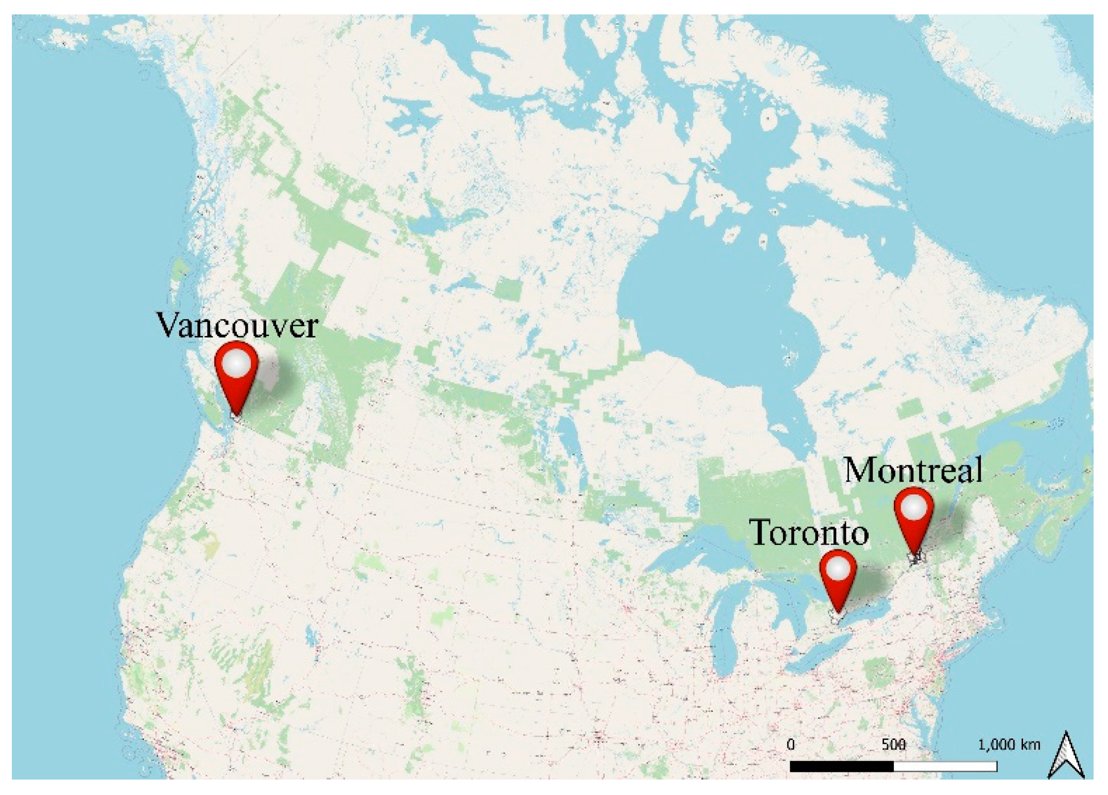
In this paper, an enhanced-IPU based algorithm was used to generate synthetic populations for the CMAs of Montreal, Toronto, and Vancouver, Canada. These three CMAs were chosen since they are the three largest Canadian CMAs in terms of population. The geographic locations of the three CMAs are shown in Figure 2.
3.2. Control Variables
A preliminary step to launching the algorithm is making the choice of variables that will be controlled along the population synthesis process. Some people and households’ attributes that are typically included in travel studies were selected. For instance, age, sex, and marital status were controlled for people, and size, type, and net income were controlled for households. The total number of people and the total number of households were also controlled for. The categories of control variables were chosen to minimize incorrect zero values as well as because of their relevance for travel studies. Table 2 summarizes the control variables and associated categories.
3.3. Zoning System
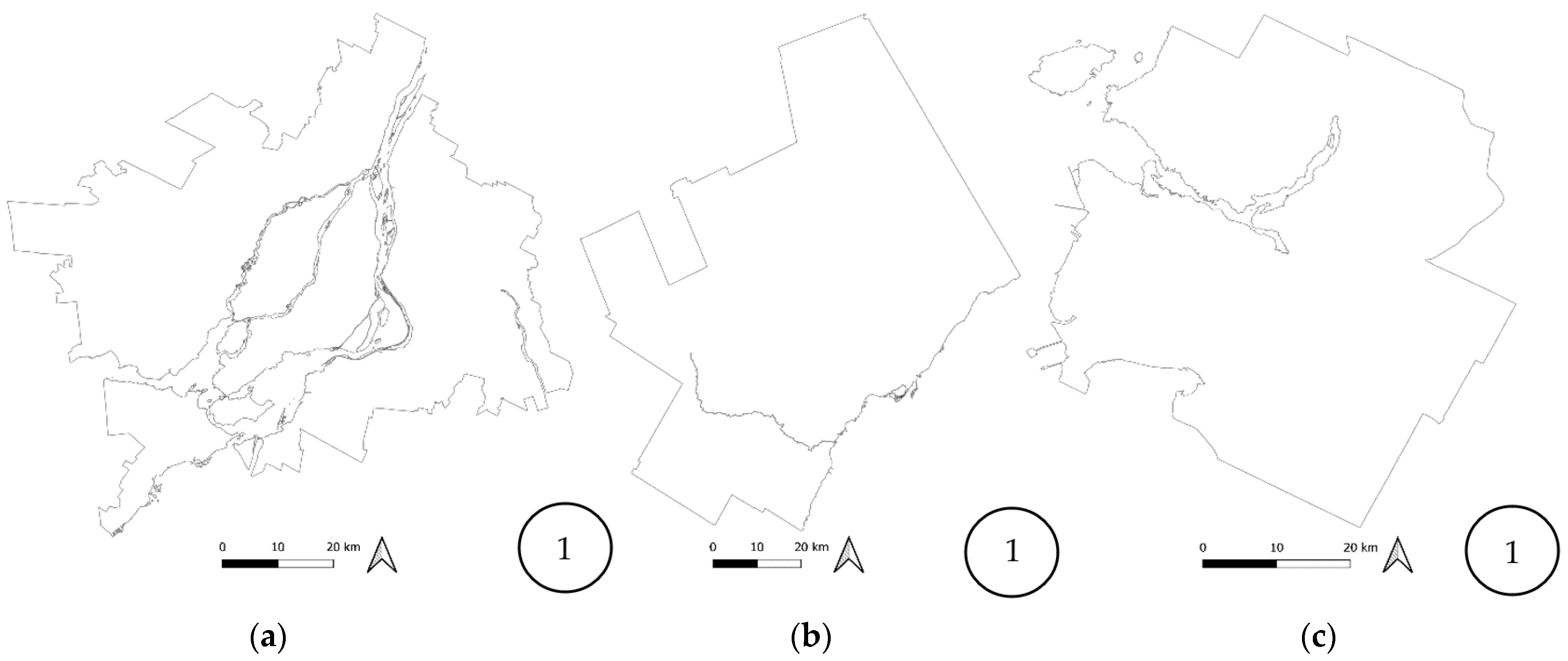
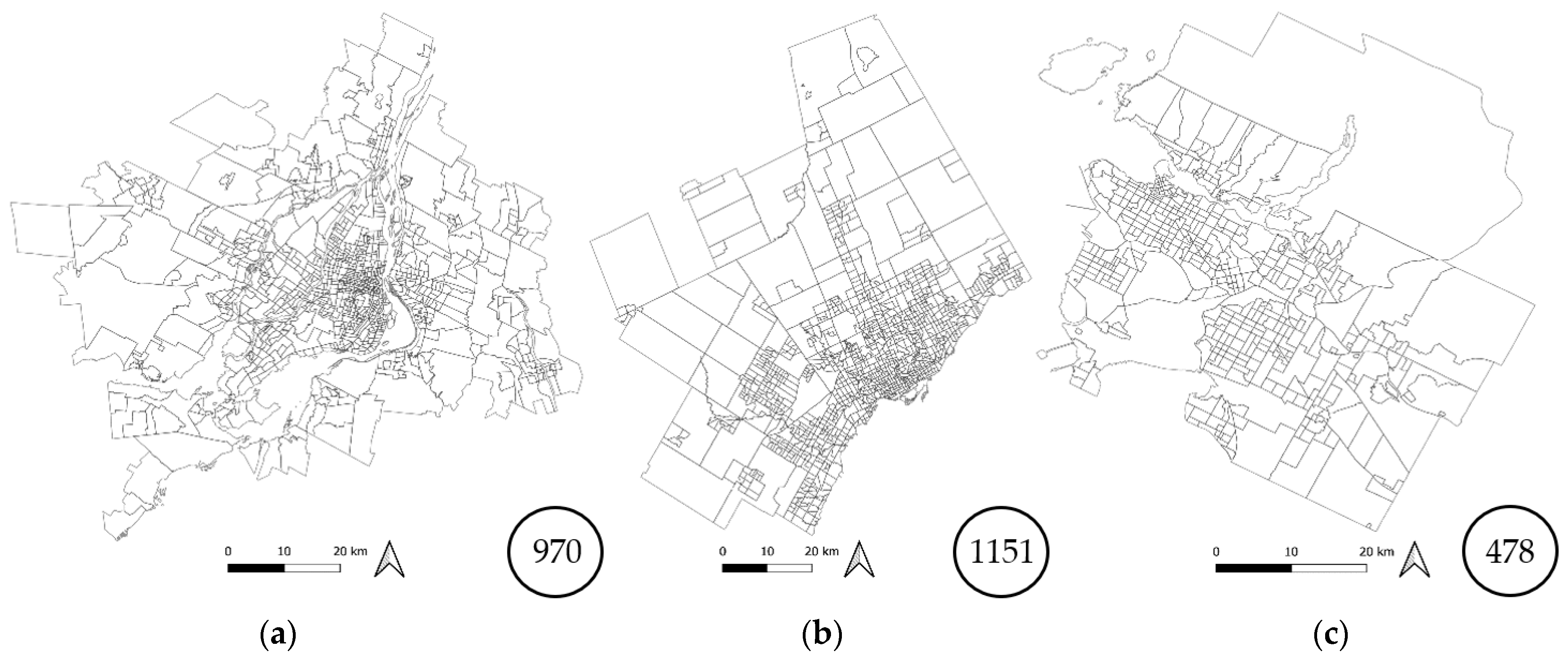
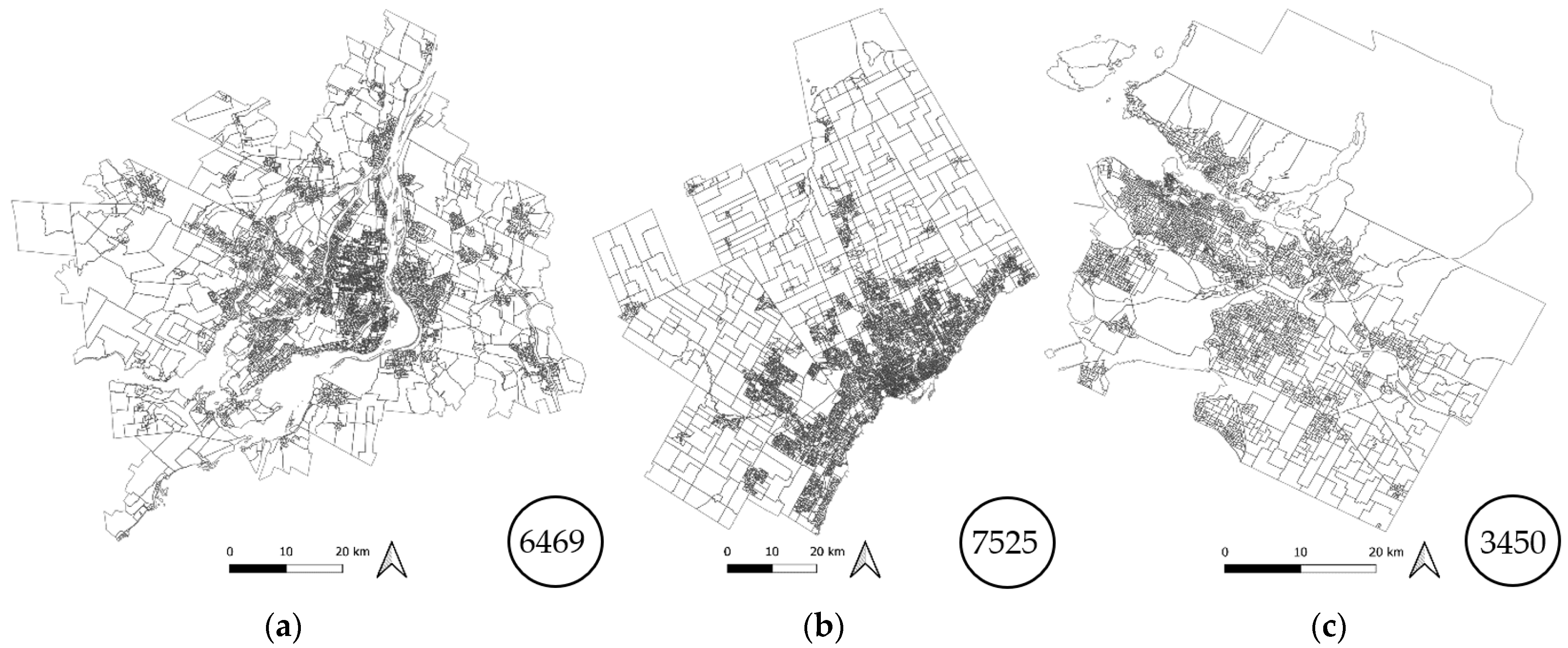
The RGRs used were selected among five standard geographic areas defined by Statistics Canada [38]. The standard geographic areas for the three CMAs are shown in Figure 3, Figure 4, Figure 5, Figure 6 and Figure 7 with the corresponding number of geographic units. They are defined—in decreasing order of aggregation—as follows:
- Census Metropolitan Area (CMA): Area with a total population of 100,000 where at least 50,000 are concentrated in a population centre [38];
- Census Subdivision (CSD): Generally equivalent to a municipality [38];
- Aggregate Dissemination Area (ADA): Area gathering 5000 to 15,000 people according to the previous census counts [38];
- Census Tract (CT): Area gathering between 2500 to 8000 people [38];
- Dissemination Area (DA): A subdivision of the CT with a population of 400 to 700 people [38].
Figure 3.
CMA boundaries for (a) Montreal, (b) Toronto, and (c) Vancouver.

Figure 4.
CSD boundaries for (a) Montreal, (b) Toronto, and (c) Vancouver.

Figure 5.
ADA boundaries for (a) Montreal, (b) Toronto, and (c) Vancouver.

Figure 6.
CT boundaries for (a) Montreal, (b) Toronto, and (c) Vancouver.

Figure 7.
DA boundaries for (a) Montreal, (b) Toronto, and (c) Vancouver.

It is important to mention that the variations of population and area between geographic resolutions are proportional. For example, each CT which is a more aggregate geographic unit than the DA in our definition, has at the same time a larger population and a larger area than each DA it contains. It is also worth mentioning that the zoning system defined is consistent, i.e., each geographic unit is included in only one geographic unit of the more aggregate geographic resolutions. For example, a DA belongs to only one CT, one ADA, one CSD, and one CMA.
3.4. Datasets
Although some sample-free population synthesizers were conceived [39,40], the majority of population synthesizers still require both aggregate (AD) and disaggregate (DD) data to be used as inputs. To perform our tests, we used datasets at different geographic resolutions from the 2016 Canadian census summary tables and PUMF. The AD used come from the 2016 Canadian census summary tables [38] while the DD were extracted from the hierarchical PUMF 2016 [38] for each CMA. The hierarchical PUMF includes a full set of demographic and socioeconomic characteristics for each people and household. Hence, an initial frequency matrix, to be expanded by enhanced IPU later [6], can easily be derived from the sample. All the data were filtered to the selected CMAs. Census summary tables were extracted for CMA, CSD, ADA, CT, and DA resolutions. However, PUMF are only available at the CMA resolution. Hence, the disaggregate sample at the CMA resolution was used to synthesize populations at less aggregate geographic resolutions. An underlying assumption of such a practice is that the correlation structure among control variables is constant across the considered geographic units [2]. However, a larger sample, i.e., having a richer pool of agents, especially when synthesizing at the finest geographic scales, helps avoid poor variance among synthesized agents.
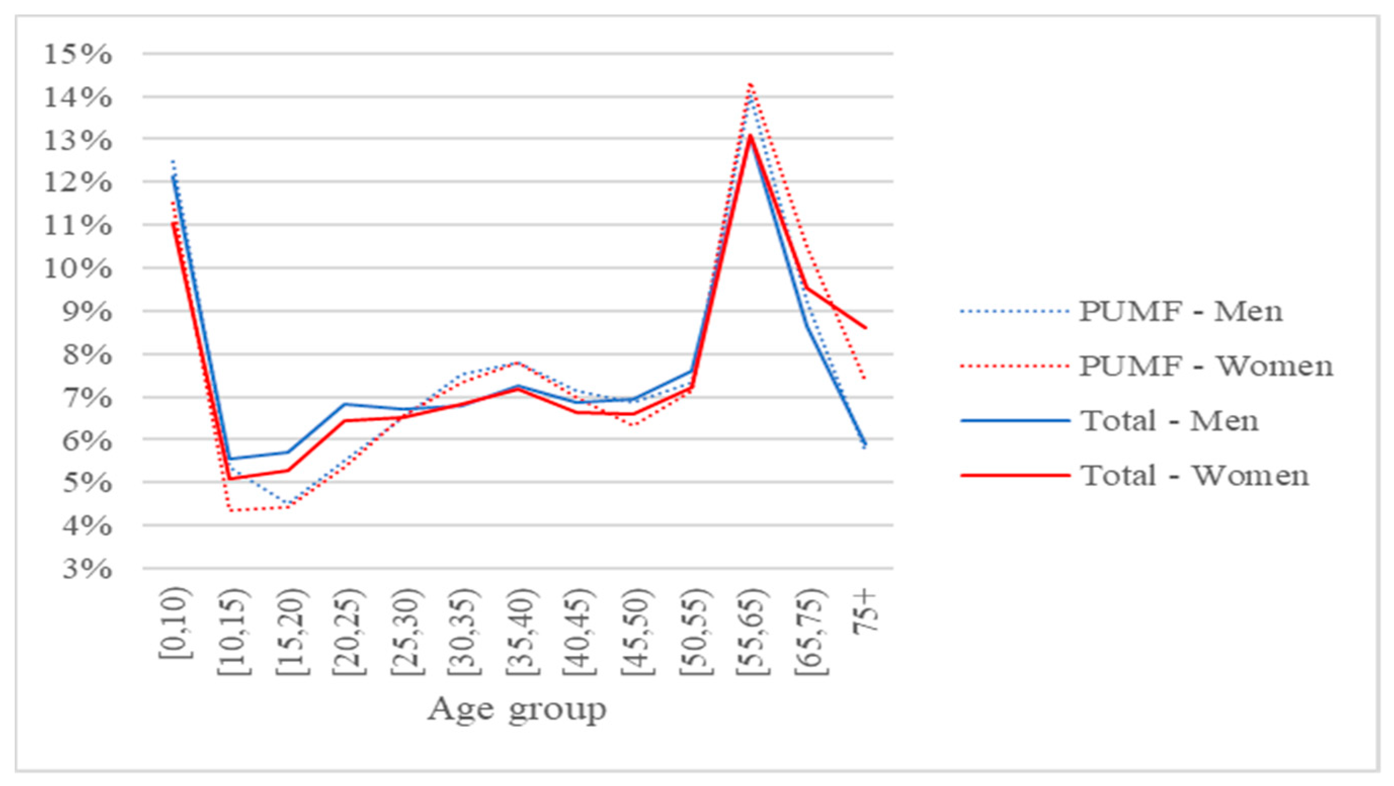
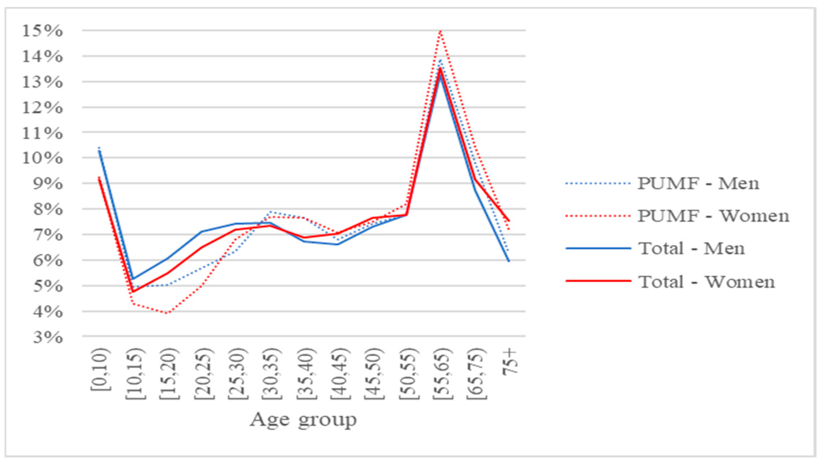
The Montreal CMA has around 4.1 million people grouped into roughly 1.7 million households. The Toronto CMA comprises around 5.9 million people in nearly 2.1 million households. The Vancouver CMA is the smallest of the three considered areas with around 2.5 million people in a little less than 1 million households. For the three CMAs, the PUMF size is about 1% of the population. A brief portrait of these areas is drawn in Figure 8, Figure 9, Figure 10, Figure 11 and Figure 12. The distributions of ages per sex in Figure 8, Figure 9 and Figure 10 were extracted from the 2016 Census PUMF and summary files. The three CMAs have similar distributions, showing peaks for people who are less than 10 years old and those who are between 55 and 65 years old. The distributions of men and women per age group are fairly similar. The PUMF sampling generally respects the distribution in the population. People between 10 and 30 years old were found to be slightly undersampled in the PUMF while people between 30 and 45 were slightly oversampled for the three CMAs.
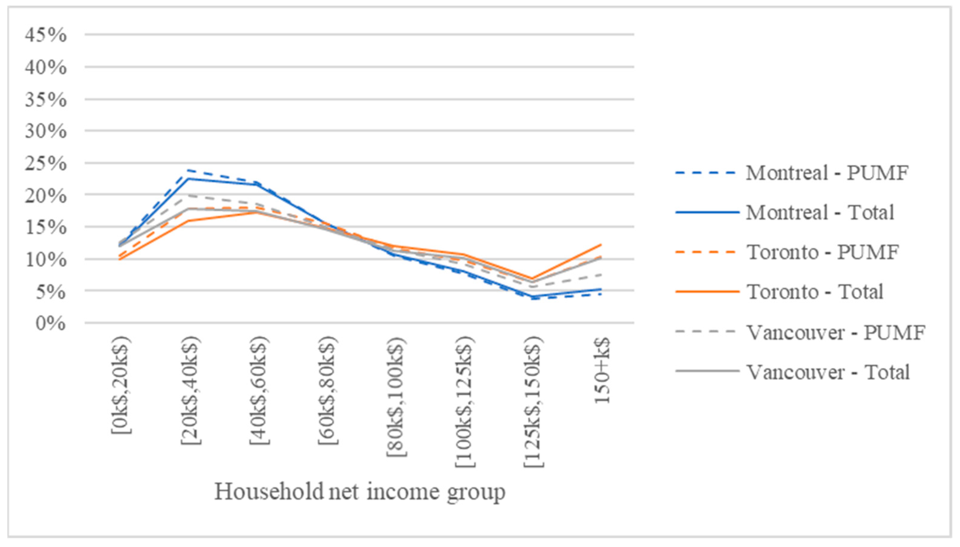
The distributions of households according to their size in the PUMF and the population of the three CMAs are shown in Figure 11. The distributions of households according to their size in the PUMF fairly followed the distributions reported in their respective populations, except for households of 5 people or more, who are noticeably underrepresented. Figure 12 exhibits the distributions of households according to their net income in the PUMF and the population of the three CMAs. No explicit divergence was detected. The distributions of the other control variables are not exhibited in this paper for the sake of brevity. However, the PUMFs were found to reflect well the distributions of the control variables in their corresponding populations.
3.5. Data Inconsistencies
It is important to note that some inconsistencies exist among the aggregate data. The census data present intra- and inter-resolution inconsistencies. The intra-resolution inconsistencies are the differences between the variables totals, e.g., the sum of men and women for the CMA being different than the sum of people belonging to all the age groups at the CMA resolution. The inter-resolution inconsistencies are the differences between the frequency of a variable category for a geographic unit and the sum of the frequencies of the same variable category for the less aggregate geographic units within it. An example of intra- and inter-resolution data inconsistencies in Montreal CMA is shown in Table 3.
Harmonization Process
To isolate the effect of these inconsistencies on the enhanced IPU-based synthesizer, harmonized census totals, i.e., census totals without intra- and inter-resolution inconsistencies, were calculated. Before describing the harmonization process, a cluster of geographic units, intra-resolution adjustments, and inter-resolution adjustments should be defined. A cluster of geographic units is comprised of all geographic units belonging to the same more aggregate geographic unit. For example, a cluster of DAs is all the DAs belonging to the same CT. An intra-resolution adjustment refers to the adjustment of categories’ frequencies of a control variable in a geographic unit so that their sum meets the total number of corresponding agents in the same geographic unit. For example, the frequencies of men and women in a CSD are proportionally adjusted so that their sum meets the total number of people in the same CSD. An inter-resolution adjustment refers to the adjustment of the frequencies of a control variable’s category in all the geographic units of a cluster, so that their sum meets the frequency of the same variable’s category at the more aggregate geographic unit they belong to. For example, the frequencies of households of three people in all the DAs of a DA’s cluster are proportionally adjusted so that their sum meets the frequency of households of three people at the corresponding CT.
The harmonization process is comprised of three steps:
- Intra-resolution adjustment of all control variables at the CMA resolution;
- Inter-resolution adjustment of hhcount and ppcount for all geographic units’ clusters at CSD, ADA, CT and DA resolutions;
- Iterative application of intra-resolution adjustment for all control variables, and inter-resolution adjustment for all geographic units’ clusters at CSD, ADA, CT, and DA resolutions, respectively. When convergence is reached at the CSD resolution, the iterative adjustment is launched at the ADA resolution and so on until the algorithm converges at the DA resolution. A convergence threshold of 10−5 is considered.
Step 3 is indeed an IPF applied to the frequencies of each variable’s categories in all the geographic units of each cluster. The goal is to fit them first, to the total of their corresponding agent within each geographic unit, then to their corresponding frequencies at the more aggregate geographic unit they belong to. For example, men frequencies at the DA resolutions are adjusted as follows (Figure 13): first, the frequencies of men and women in each DA are proportionally adjusted so that their sum meets the total number of people in the same DA. Then, the men’s frequency in each DA undergoes a proportional adjustment so that the sum of men’s frequencies in each cluster of DAs meets the men’s frequency at the corresponding CT. The process is then iteratively repeated until the frequencies of all variable categories at the DA resolution meet both constraints within a convergence threshold. Harmonized datasets, i.e., datasets without intra- and inter-resolution inconsistencies, are thus obtained for the five geographic resolutions considered.
3.6. Scenarios
As mentioned previously, the enhanced IPU algorithm [6] can simultaneously take into consideration two geographic resolutions for households and people attributes. In this paper, the REGION was always set to the CMA when a double control was applied. This is because the fitting errors are better assessed at the CMA resolution, as explained in the Introduction; thus, adding controls at the CMA resolution would be the best way to reduce fitting errors. Using the enhanced IPU algorithm implemented in PopGen2.0 [41], 18 synthetic populations were generated for each CMA according to the scenarios enumerated in Table 4. Scenarios with harmonized data were tested to assess the effect of intra- and inter-resolution inconsistencies. Scenarios with two controlled resolutions were compared to scenarios with a single controlled resolution to show the impact of the additional control at the CMA resolution.
Accuracy and Precision
For each synthetic population generated, the accuracy and the precision were assessed. The accuracy reflects the representativeness of the sociodemographic characteristics of the entire population and is measured by the fit of the total synthetic population to the targets at the CMA resolution. Hence, the sum of estimated frequencies of each variable’s category across the RGUs was calculated and compared to the observed frequency of the same variable’s category at the CMA resolution. For example, the sum of synthetic men across DAs was calculated and compared to the frequency of men at the CMA level.
The precision reflects the representativeness of the real population’s spatial heterogeneity. Precision assessment requires prior data processing. The frequencies of variables’ categories were first interpolated from each RGU to the DAs within it. The interpolation was done proportionally to the distribution of the RGU’s households on the DAs within it. This is because the household is the main synthesis agent for the enhanced IPU algorithm. The calculations were performed according to the following formula:
where
- i denotes the ith variable category;
- j denotes the jth DA within the RGU;
- RGU refers to a reference geographic unit;
- refers to the frequency of the ith variable category in an RGU, as estimated by the enhanced IPU;
- refers to the interpolated frequency of the ith variable category in the jth DA;
- refers to the households’ count in the jth DA;
- refers to the households’ count in the RGU.
Then, a synthetic population was drawn for each DA using the interpolated frequencies. This can be done using the “synthesize” function in the ipfr R package [42]. The frequencies of variables’ categories were compared to the census targets for each DA, and the more similar they were, the more precise was the synthetic population. The mathematical formulas for fitting and spatialization errors calculations are detailed in Section 3.7. The higher the fitting errors, the less accurate the synthetic population was, and the higher the spatialization errors, the less precise was the synthetic population.
As stated previously, the main objective was to assess the impact of the RGR’s choice on the enhanced IPU algorithm performance to provide insights into the best compromise between precision and accuracy. The variables were controlled in the same order for all scenarios with the people counts being the last variable to be fitted. The 18 scenarios were run for the CMAs of Montreal, Toronto, and Vancouver.
3.7. Assessment Criteria
Three indicators were calculated to assess the various scenarios: census inter-resolution inconsistencies, fitting errors, and spatialization errors. These criteria are described below. As we were interested in a good fit of households and people, errors on both types of agents were integrated in the formulas. Moreover, the indicators were calculated per 1000 agents. They were made relative to the number of agents in order to keep the results of the three CMAs comparable, as they have drastically different sizes of populations. Finally, as the selection step was not deterministic [4], i.e., the synthetic population differed for each simulation, the indicators were calculated on synthetic populations that were averaged across 50 simulations to allow for general conclusions.
3.7.1. Census Inter-Resolution Inconsistencies (α)
As described previously, the census inter-resolution inconsistencies indicator was calculated as the sum of the absolute values of the differences between the observed frequency of each variable’s category in a geographic unit and the sum of the observed frequencies of the same variable’s category in the less aggregate geographic units within it. As the census targets at the CMA resolution were the most reliable, the inter-resolution inconsistencies were calculated relative to the CMA resolution as per the following formula:
where
- i denotes the ith variable category i = 1 … m;
- j denotes the jth RGU j = 1 … n;
- refers to the observed frequency of the ith variable category in the jth RGU;
- refers to the observed frequency of the ith variable category in the CMA;
- refers to the households’ count in the CMA;
- refers to the people’s count in the CMA.
3.7.2. Fitting Errors (β)
The fitting errors formula is similar to the census inter-resolution inconsistencies one, except for the differences being calculated between the observed frequencies of each variable’s category in a geographic unit, and the sum of the simulated frequencies of the same variable’s category in the less aggregate geographic units within it. The fitting errors were calculated as follows:
where
- i denotes the ith variable category i = 1 … m;
- j denotes the jth RGU j = 1 … n;
- refers to the simulated frequency of the ith variable category in the jth RGU;
- refers to the observed frequency of the ith variable category in the CMA;
- refers to the households’ count in the CMA;
- refers to the people’s count in the CMA.
3.7.3. Spatialization Errors (γ)
To measure the spatialization errors, the absolute differences between the simulated frequencies of the variable categories interpolated at the DA resolution () and the observed frequencies of the variable categories at the DA resolution were calculated, then summed over all the variable categories and the DAs as follows:
where
- i denotes the ith variable category i = 1 … m;
- j denotes the jth RGU j = 1 … n;
- refers to the interpolated simulated frequency of the ith variable category in the jth DA;
- refers to the observed frequency of the ith variable category in the jth DA;
- refers to the households’ count in the CMA;
- refers to the people’s count in the CMA.
4. Results
In this section, different groups of the 18 generated synthetic populations were compared. This provides insights into how the accuracy and the precision of the synthetic population were impacted by (1) the RGR’s aggregation, (2) the data inconsistencies between census geographic resolutions, and (3) the multiple geographic resolutions control. Means to improve both accuracy and precision of synthetic populations are then suggested.
4.1. How Do α, β, and γ Vary According to the RGR Used?
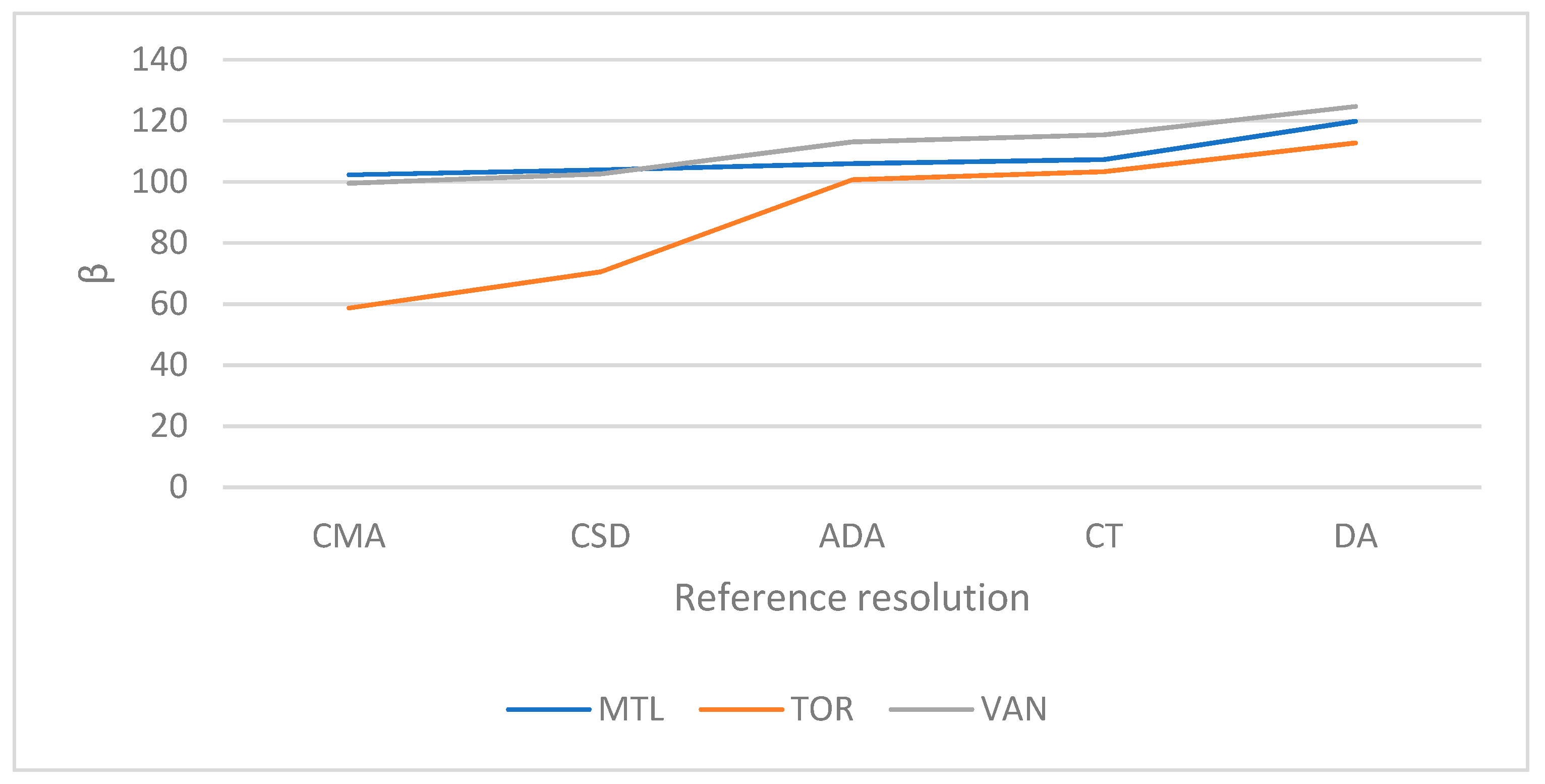
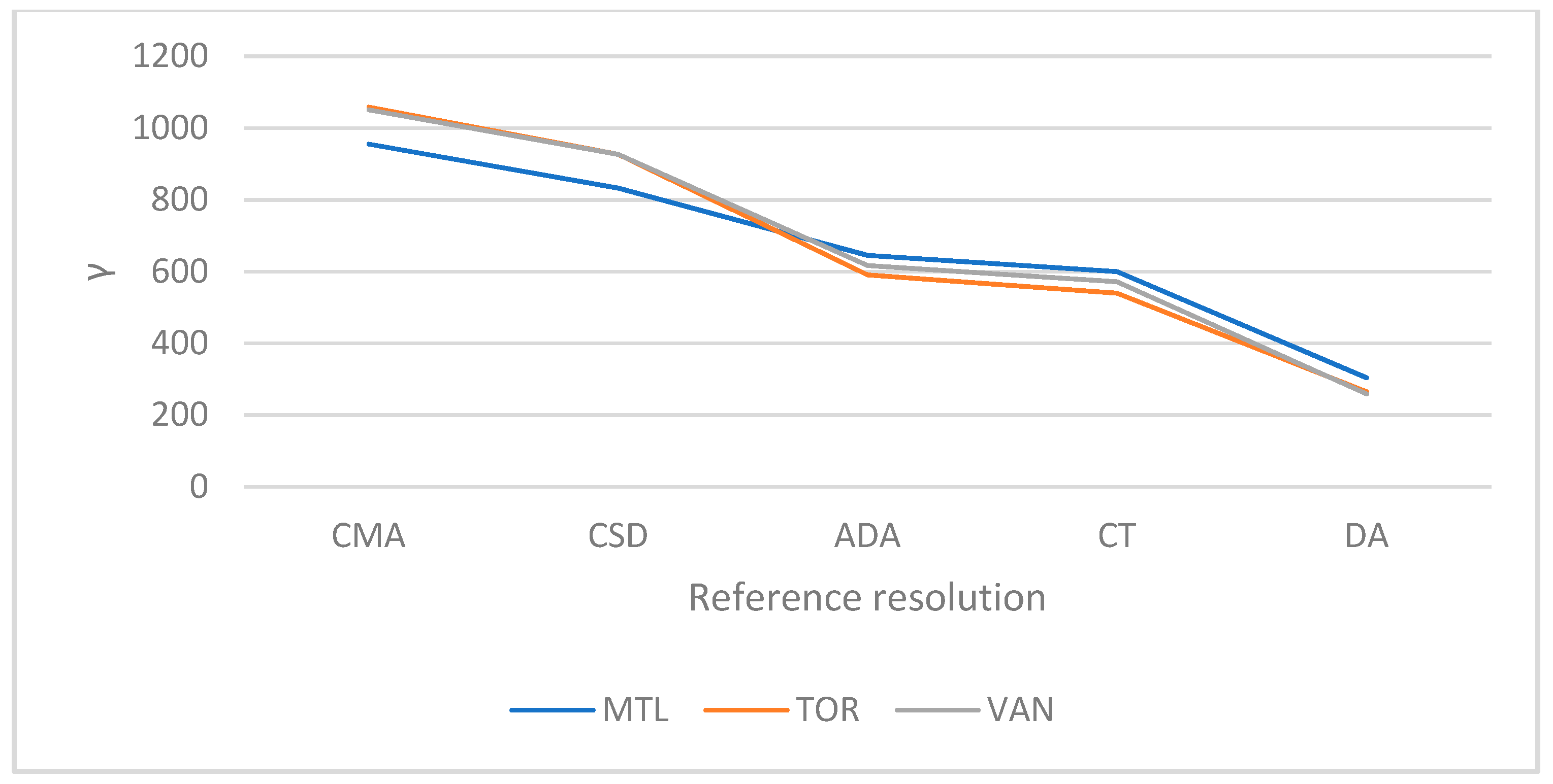
The variations of α, β, and γ according to the RGR are depicted in Figure 14, Figure 15 and Figure 16. The indicators generally show the expected trends, with the three CMAs showing similar results for each indicator.
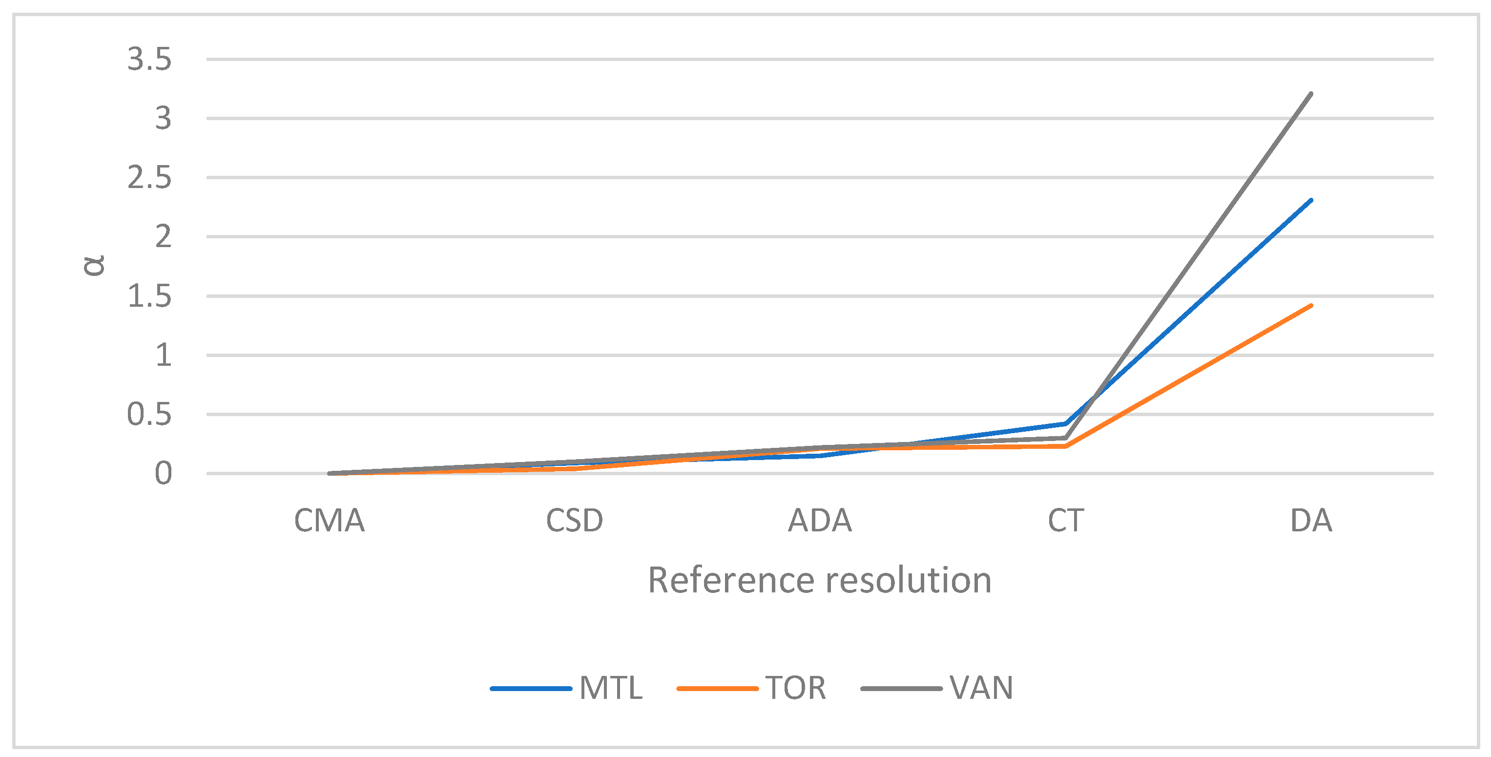
α increased when the RGR became less aggregate, i.e., when the number of RGUs increased. In fact, the less aggregate the geographic unit is, the more rounded frequencies for privacy issues are likely to occur in the census data, thus yielding higher inter-resolution inconsistencies. α was, however, found to be of relatively low magnitude ranging from 0 at the CMA resolution to less than 3.5 at the DA resolution.
β also increased when the RGR became less aggregate for the three CMAs. This is also expected since both the inter-resolution inconsistencies (α) and the synthesis exercise complexity increased when the RGR became less aggregate, thus impacting the accuracy of the synthetic population. When synthesizing at the CMA resolution, only one set of census targets has to be met, compared to 6469 sets of targets at the DA level for Montreal, more than 7525 for Toronto, and more than 3450 for Vancouver. This makes the synthesis exercise more complex at this level and thus potential fitting errors multiply. It is important to mention that the problem of incorrect zero cells, more important at less aggregate resolutions, does not explain the variation of fitting errors in our case since the PUMF was always taken at the CMA level. However, the zero marginals problem, mainly due to rounding for privacy issues, is in itself a challenge for fitting-based synthesizers convergence, apart from increasing α, and thus is damaging the synthetic population’s accuracy. β was found to range from a minimum of around 60 (Toronto) at the CMA level to around 120 at the DA level. A lower β was observed for Toronto at the CMA and CSD levels when compared to Montreal and Vancouver. The fluctuation of the corner solution found by the algorithm is a plausible explanation. However, quantifying the impact of the CMA’s structure in terms of types of households and people on the corner solution is beyond the scope of this paper. However, the β maximum values at the DA resolution, being fairly similar for the three CMAs, provide insight on the cost in terms of fitting errors of synthesizing at the least aggregate geographic resolution.
γ was found to decrease with a less aggregate RGR. This is expected since higher aggregation results in a stronger spatial homogeneity assumption and thus a less precise synthetic population. The spatial homogeneity assumption became stronger with more aggregate RGRs because a large population over a wide area is more likely to be spatially heterogeneous than a small population over a compact area. The three CMAs showed similar trends and values with the maximum γ being around 1000 at the CMA resolution and the minimum around 300 at the DA resolution. Two observations are worth mentioning: first, the spatialization errors’ magnitude was higher than the fitting errors’ magnitude for the same synthesis area (the CMA). Second, the ratio of the highest error to the lowest error was higher than 3 for spatialization errors, while it remained lower than 2 for fitting errors (1.2 if calculated for Montreal and Vancouver). This shows that a synthetic population is generally susceptible to more spatialization errors than fitting errors. Hence, for the same synthesis area, perfect precision is more difficult to achieve than perfect accuracy. Moreover, it shows that the gain in terms of precision when synthesizing at the least aggregate RGR is more important than the loss in terms of accuracy and vice-versa.
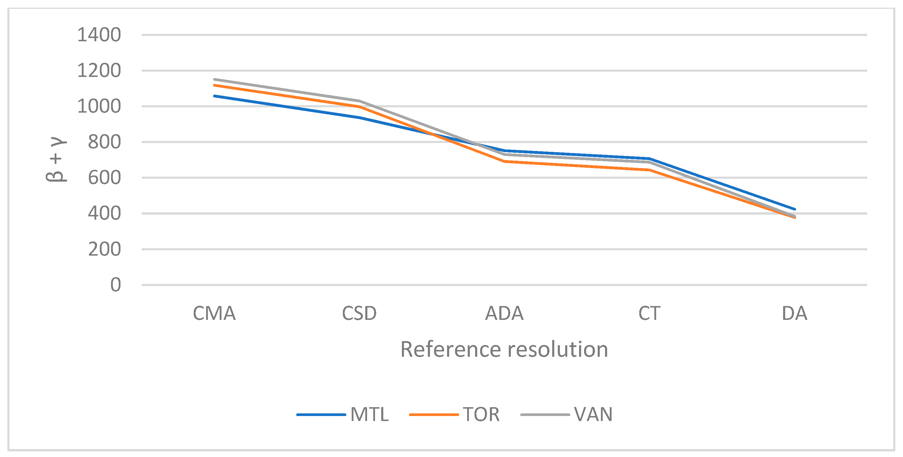
As we were interested in optimizing both accuracy and precision, i.e., minimizing both fitting and spatialization errors, the variation of the total error (β + γ) according to the RGR used was calculated as depicted in Figure 17.
The synthetic populations at the DA resolution showed around 400 total errors per 1000 agents, while at the CMA resolution around 1100 errors per 1000 agents were observed. The total error was reduced by nearly 64% at the DA resolution. Hence, using the DA as the RGR was shown to be the best compromise between fitting and spatialization errors. In other words, using the DA as the RGR allows the quality, i.e., the combination of accuracy and precision, of the synthetic population to be optimized.
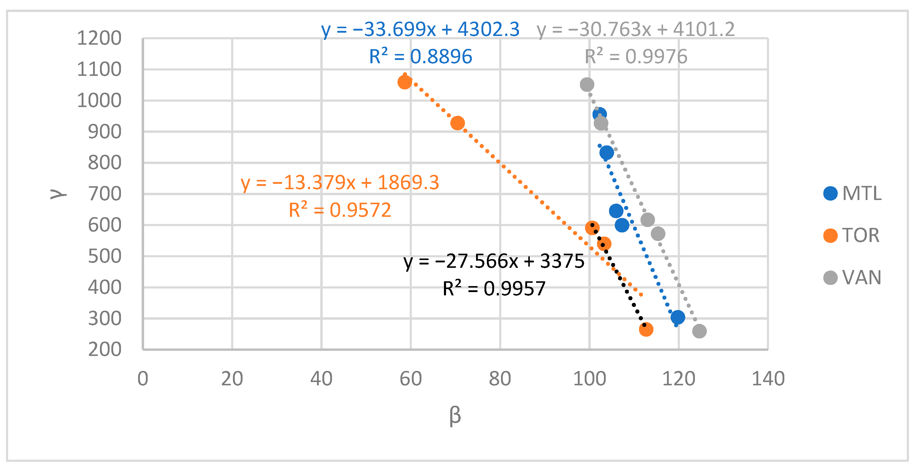
4.2. How Does γ Vary according to β? In Other Words, How Is the Precision Improved When Decreasing Accuracy, i.e., When Using a Less Aggregate RGR, and Vice-Versa?
β was found to increase and γ to decrease when the RGR became less aggregate. The variation of γ according to β was then further investigated in the three CMAs (Figure 18). The relation between γ and β could be fitted well by a decreasing linear trend as evidenced by the high R2 calculated. For Montreal and Vancouver, when the RGR decreased, each additional fitting error per 1000 agents gave in return around 30 less spatialization errors per 1000 agents. For Toronto, each additional fitting error per 1000 agents was found to give in return around 13 spatialization errors per 1000 agents. However, Toronto’s divergence from Montreal and Vancouver was mainly due to its low β errors at the CMA and CSD resolutions as shown in Figure 15. If the errors at CMA and CSD resolutions for Toronto are neglected, the slope of the trendline fitting the variation of γ according to β (black trendline) becomes similar to that of Montreal and Vancouver.
The key takeaway of this analysis is the decreasing linear variation of γ according to β with a single fitting error being equivalent to at least 13 spatialization errors per 1000 agents. The minimal total error was thus found at the DA resolution because the decrease of spatialization errors when the RGR became less aggregate was much higher than the increase of fitting errors. In other words, γ errors are more sensitive to the RGR aggregation than β errors.
4.3. What Is the Impact of Census Targets’ Harmonization and Additional Control at the CMA Resolution on the Total Error?
In the quest for an optimal synthetic population, i.e., a synthetic population with minimum β + γ error, the following four configurations were tested:
- 1R: Raw data with single control;
- 2R: Raw data with double control;
- 1H: Harmonized data with single control;
- 2H: Harmonized data with double control.
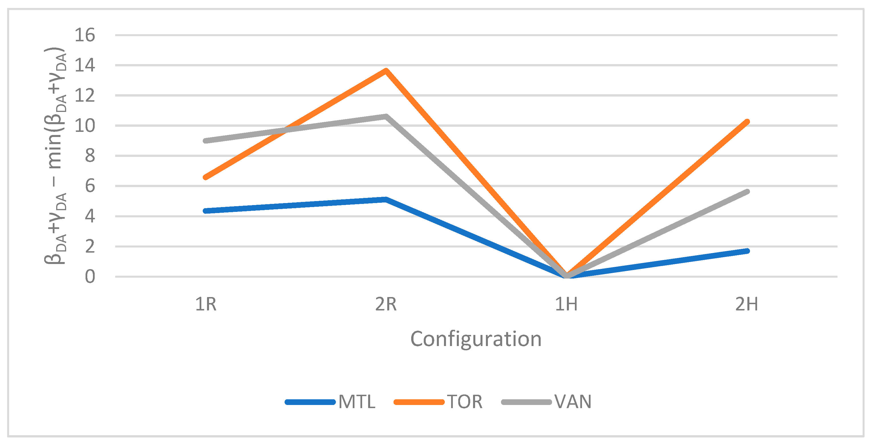
The variation of the total error according to each configuration was assessed. As the DA resolution was found to minimize the total error, the different configurations’ results at the DA resolution are shown in Figure 19. The goal was to detect which configuration would help to further reduce the total error, i.e., further optimize the synthetic population.
The total errors were lower for the 1H and 2H scenarios compared to those of 1R and 2R. This shows that harmonizing census targets helps in improving the quality of the synthetic population. This is mainly due to the intra- and inter-resolution inconsistencies between all geographic resolutions being reduced to zero. However, 2R and 2H showed higher total errors than 1R and 1H, respectively. In fact, the double control improved the synthetic population’s fit at the REGION resolution, thus damaging its fit at the GEO resolution. As shown in Figure 18, when β varies, γ undergoes an opposite, more important, variation. Hence, as the double control applied improves the fit at the CMA resolution, i.e., reduces β errors, γ errors undergo an increase the magnitude of which is more important than β errors reduction, and the total error thus increases. In summary, harmonizing census targets helps improve the synthetic population’s quality. The total error reduction obtained ranged from ~4 to ~9 errors per 1000 agents in the study area’s CMAs.
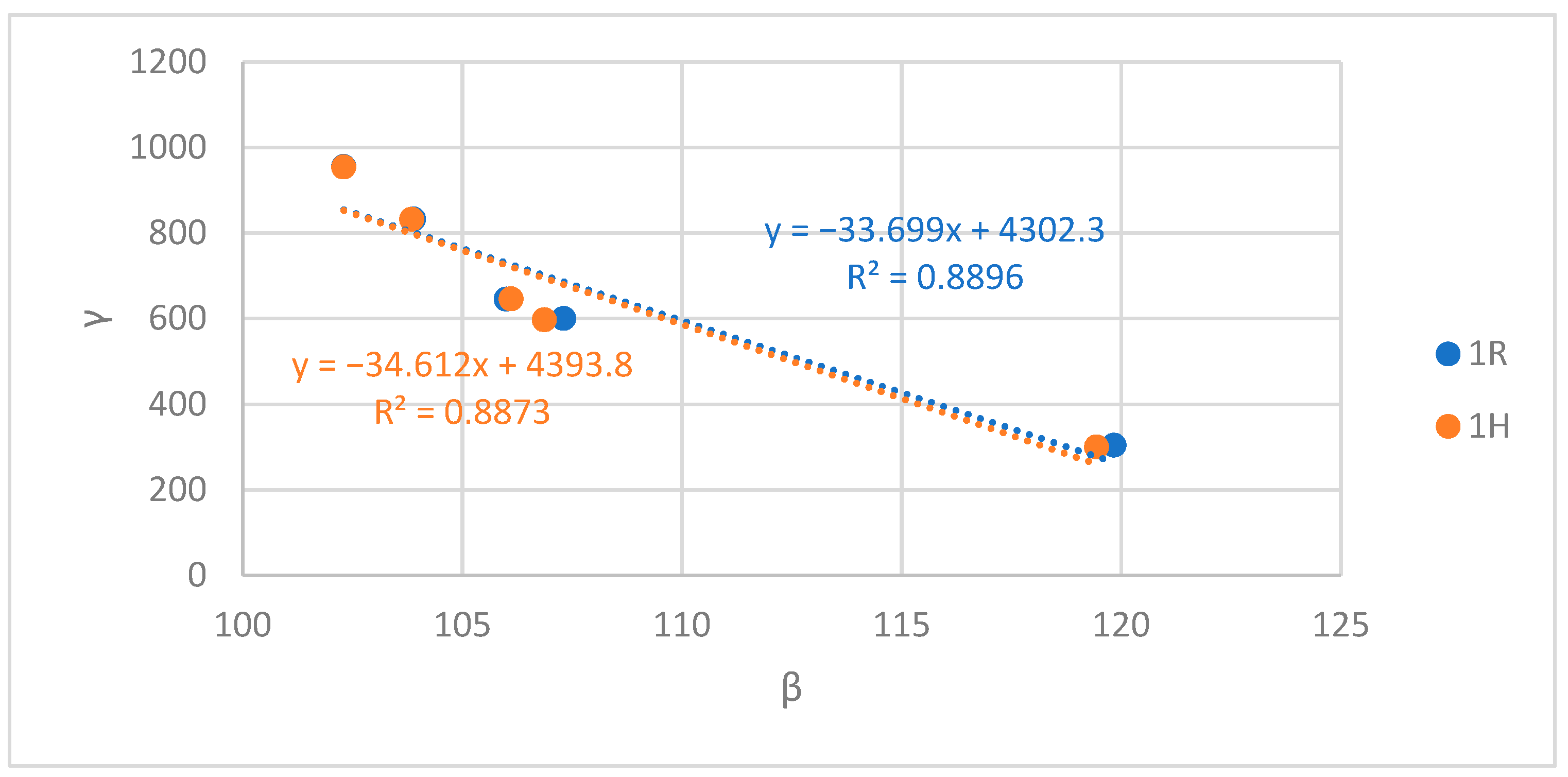
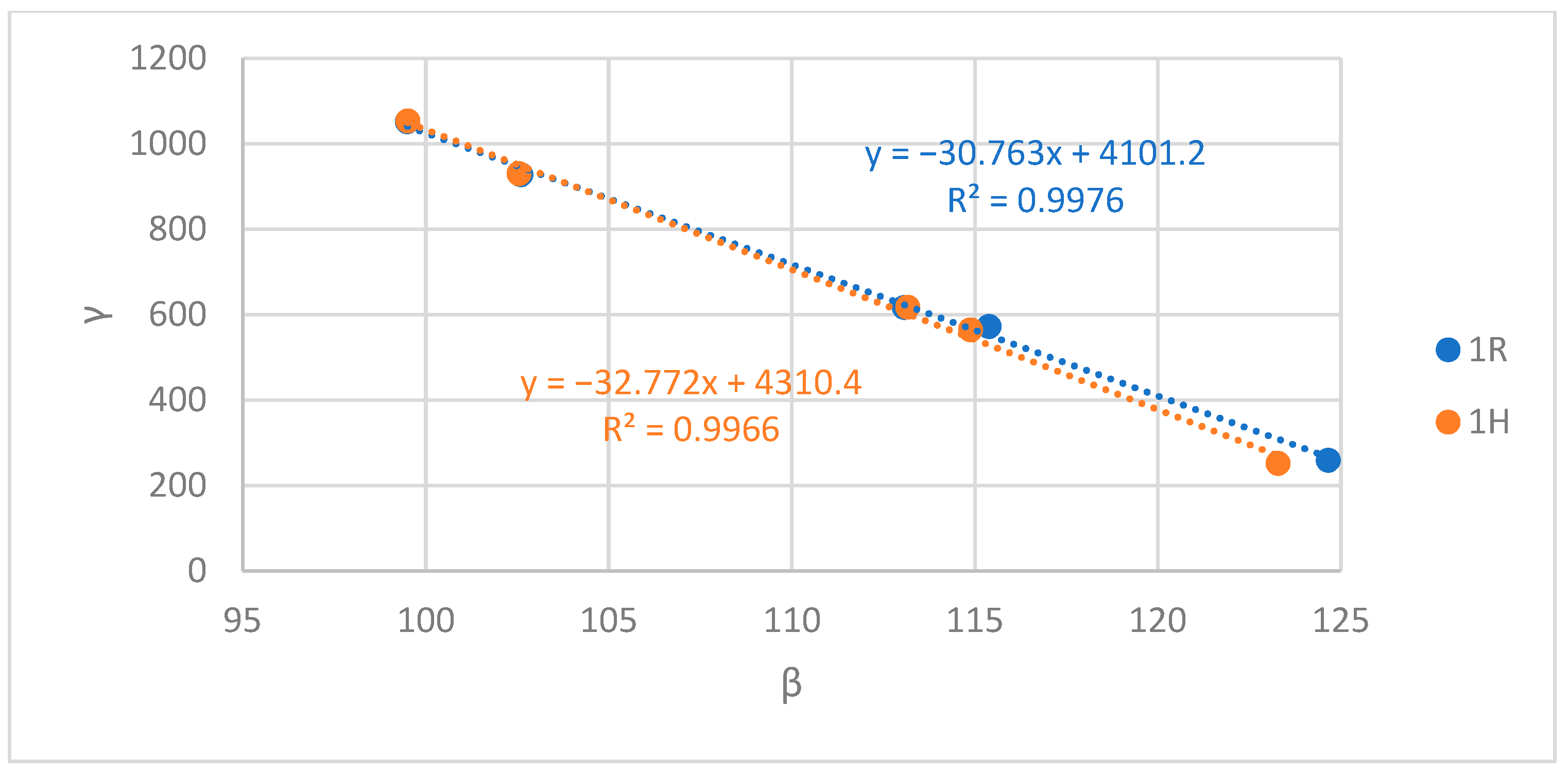
4.4. How Does the Variation of γ According to β Change When Census Targets Are Harmonized?
Figure 20, Figure 21 and Figure 22 show the variation of γ according to β for the 1R and 1H configurations in Montreal, Toronto, and Vancouver CMAs, respectively. The goal was to assess how this variation is altered when harmonized census targets are used. For the three CMAs, the absolute value of the slope of the 1H trendline was higher than the absolute value of the slope of the 1R trendline. This means that when census targets are harmonized, for an additional fitting error we get a higher reduction of spatialization errors. Hence, synthesizing at a less aggregate RGR becomes more beneficial with harmonized census targets as the γ error, and thus the total error, are further reduced for the same β error increase.
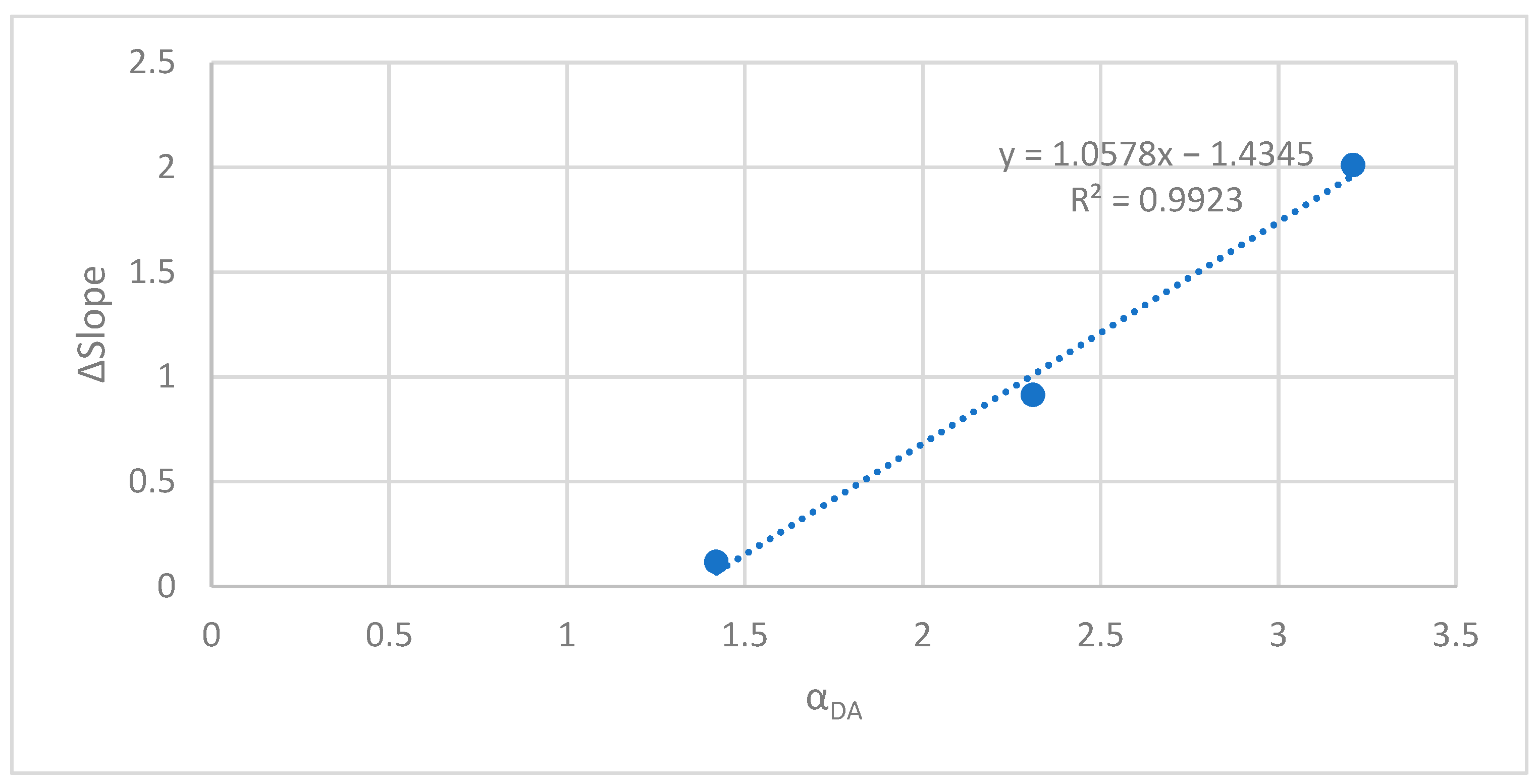
For each CMA, the difference between the 1R trendline slope and the 1H trendline slope (ΔSlope) was calculated, and its variation according to the inter-resolution inconsistencies at the DA resolution (αDA) is depicted in Figure 23. The variation was found to be linear, with the ΔSlope increasing when the αDA increases. This means that the more inter-resolution inconsistencies a CMA shows, the more harmonizing its census targets allows to save spatialization errors for each additional fitting error, i.e., when decreasing the RGR. In other words, the more inter-resolution inconsistencies a CMA shows, the more harmonization helps to increase its synthetic population’s accuracy for the same cost in terms of precision.
5. Discussion
A synthetic population’s quality is usually assessed by its fit to the census targets at the RGR [2,4,6,7,9,10]. This paper introduced the concepts of sociodemographic accuracy and spatial precision as components of the quality measure. The accuracy of the synthetic population (representativeness of the sociodemographic characteristics of the entire population) was measured by its fit to the census targets at the CMA resolution. This is because the census targets at the CMA resolution are considered as the ground truth due to the rare or non-existent need to adjust census targets to preserve privacy at this level. To measure the precision (representativeness of the real population’s spatial heterogeneity), the synthetic population was first interpolated from its RGR to the DA resolution. The precision was measured by the fit of the interpolated population to the census targets at the DA resolution. Fitting errors (β) and spatialization errors (γ) were thus calculated to assess accuracy and precision, respectively. An optimal synthetic population is a synthetic population showing minimal total (β + γ) error.
While population synthesizers are continually conceived to improve the quality of population synthesis, the choice of the RGR and its impact on the quality of synthetic populations have not been studied to the best of our knowledge. Hence, another contribution of this paper was its assessment of the impact of the RGR characteristics on the quality of population synthesis. The main characteristics of the RGR considered are its aggregation and the inter-resolution inconsistencies (α) it shows. β was found to increase and γ to decrease with less aggregate geographic resolutions, with γ magnitude being generally more important than β. γ was also found to be more sensitive to the RGR’s aggregation than β, thus yielding a minimal total error at the least aggregate RGR.
An additional contribution of this paper was its testing of the impact of double control and census targets’ harmonization on the quality of the synthetic population. While double control is originally introduced to control variables that are not available at the same geographic resolution [6], we tested it as a plausible means of reducing the total error since it makes it possible to control the least and the most aggregate geographic resolutions simultaneously, i.e., the resolutions where γ and β are respectively measured. In their paper, Konduri et al. showed that double control improves the quality of the synthetic population [6]. The quality indicator they used comprises only the fit at the more aggregate level [6], which corresponds to accuracy in this paper. However, we found that the double control damages the quality of the synthetic population when both accuracy and spatial precision are considered as components of the quality indicator. In fact, when correcting the fit to the most aggregate geographic resolution (reducing β), the fit to the least aggregate resolution was compromised (γ increased). As γ variation is more important than β variation, the total error increased, hence damaging the synthetic population’s quality. On the contrary, census targets’ harmonization, i.e., applying proportional adjustments to census targets to reduce intra- and inter-resolution inconsistencies to zero, was found to improve the quality of the synthetic population. Moreover, for the same β, a lower γ was obtained when population synthesis was performed using harmonized census targets. It is worth mentioning that despite the importance of intra- [25] and inter-resolution [6] consistency for population synthesizers being mentioned in the literature, quantifying the impact of such inconsistencies, both in terms of accuracy and precision, and suggesting a complete framework to harmonize census data within and between resolutions simultaneously were, to the best of our knowledge, done for the first time in this paper.
6. Conclusions
In this paper, the enhanced IPU algorithm [6] was used to synthesize populations at five RGRs (CMA, CSD, ADA, CT, and DA) for the CMAs of Montreal, Toronto, and Vancouver. Eighteen scenarios involving different RGRs, data types (raw or harmonized), and control types (single or double) were compared to assess the impact of the RGR characteristics on the quality of population synthesis. Specifically, the impact of the following factors on the synthetic populations’ accuracy and precision was assessed: (1) the aggregation of the RGR, (2) data inconsistencies between census geographic resolutions, and (3) multiple geographic resolutions control.
Three indicators were calculated to compare the synthetic populations generated: census inter-resolution inconsistencies (α), fitting errors (β), and spatialization errors (γ). The impact on the three indicators of the RGR was first investigated. α and β were found to increase, and γ to decrease when the RGR became less aggregate. The total error was found to decrease when the RGR became less aggregate yielding, an optimal synthetic population at the DA resolution. Then, the variation of γ according to β was investigated. A decreasing linear trend was observed with an important slope, meaning that spatialization errors are more sensitive to the RGR than fitting errors. Finally, the impacts of harmonization and double control were assessed. The double control was found to damage the quality of the synthetic population while the harmonization was found to reduce the total error. The harmonization was also found to be more effective when the census inconsistencies were higher. In summary, synthesizing a population at the DA resolution using harmonized census targets was found to be the best practice.
The main limitation of the conclusions of this paper lies in the number of CMAs investigated. Although finding similar trends for three large and different CMAs allows for conclusions to be made, they would be better founded if based on a larger number of CMAs. Next steps involve comparing the impacts of the RGR choice on various population synthesizers, considering the spatial precision as a component of the synthetic population’s quality measure. Various spatialization approaches to allocate the synthetic households to individual dwellings should then be tested on a synthetic population with the best accuracy and precision possible.
Author Contributions
Study conception and design, Mohamed Khachman, Catherine Morency, and Francesco Ciari; analysis and interpretation of results, Mohamed Khachman; draft manuscript preparation, Mohamed Khachman, Catherine Morency, and Francesco Ciari. All authors have read and agreed to the published version of the manuscript.
Funding
The authors wish to acknowledge the contribution and financial support of the Mobilité research chair partners: Ministère des transports du Québec (MTQ), Société de Transport de Montréal (STM), Autorité Régionale de Transport Métropolitain, exo, and Ville de Montréal.
Data Availability Statement
Publicly available datasets were analyzed in this study. This data can be found here: https://www12.statcan.gc.ca/census-recensement/2016/dp-pd/index-eng.cfm (accessed on 12 November 2021).
Conflicts of Interest
The authors declare no conflict of interest.
References
- Mohammadian, A.; Javanmardi, M.; Zhang, Y. Synthetic household travel survey data simulation. Transp. Res. Part C Emerg. Technol. 2010, 18, 869–878. [Google Scholar] [CrossRef]
- Beckman, R.J.; Baggerly, K.A.; McKay, M.D. Creating synthetic baseline populations. Transp. Res. Part A Policy Pract. 1996, 30, 415–429. [Google Scholar] [CrossRef]
- Deming, W.E.; Stephan, F.F. On a least squares adjustment of a sampled frequency table when the expected marginal totals are known. Ann. Math. Stat. 1940, 11, 427–444. [Google Scholar] [CrossRef]
- Ye, X.; Konduri, K.; Pendyala, R.M.; Sana, B.; Waddell, P. A methodology to match distributions of both household and person attributes in the generation of synthetic populations. In Proceedings of the 88th Annual Meeting of the Transportation Research Board, Washington, DC, USA, 11–15 January 2009. [Google Scholar]
- Fournier, N.; Christopha, E.; Akkinepally, A.P.; Azevedo, C.L. Integrated population synthesis and workplace assignment using an efficient optimization-based person-household matching method. Transportation 2020, 48, 1061–1087. [Google Scholar] [CrossRef]
- Konduri, K.C.; You, D.; Garikapati, V.M.; Pendyala, R.M. Enhanced synthetic population generator that accommodates control variables at multiple geographic resolutions. Transp. Res. Rec. J. Transp. Res. Board 2016, 2563, 40–50. [Google Scholar] [CrossRef] [Green Version]
- Moreno, A.T.; Moeckel, R. Population Synthesis Handling Three Geographical Resolutions. ISPRS Int. J. Geoinf. 2018, 7, 174. [Google Scholar] [CrossRef] [Green Version]
- Hunsinger, E.; Alaska Department of Labor and Workforce Development. Iterative Proportional Fitting for A Two-Dimensional Table. 2008. Available online: https://edyhsgr.github.io/IPFDescription/AKDOLWDIPFTWOD.pdf (accessed on 15 July 2018).
- Guo, J.; Bhat, C. Population synthesis for microsimulating travel behavior. Transp. Res. Rec. J. Transp. Res. Board 2007, 2014, 92–101. [Google Scholar] [CrossRef] [Green Version]
- Auld, J.A.; Mohammadian, A.; Wies, K. Population synthesis with subregion-level control variable aggregation. J. Transp. Eng. 2009, 135, 632–639. [Google Scholar] [CrossRef]
- Müller, K.; Axhausen, K.W. Population Synthesis for Microsimulation: State of the Art. Arb. Verk. Raumplan. 2010, 638, 1–15. [Google Scholar]
- Farooq, B.; Bierlaire, M.; Hurtubia, R.; Flötteröd, G. Simulation Based Population Synthesis. Transportation 2013, 58, 243–263. [Google Scholar] [CrossRef] [Green Version]
- Williamson, P.; Birkin, M.; Rees, P.H. The estimation of population microdata by using data from small area statistics and samples of anonymized records. Environ. Plan A. 1998, 30, 785–816. [Google Scholar] [CrossRef] [PubMed]
- Arentze, T.; Timmermans, H.; Hofman, F. Creating Synthetic Household Populations: Problems and Approach. Transp. Res. Rec. J. Transp. Res. Board 2007, 2014, 85–91. [Google Scholar] [CrossRef]
- Yaméogo, B.F.; Gastineau, P.; Hankach, P.; Vandanjon, P.O. Comparing Methods for Generating a Two-layered Synthetic Population. Transp. Res. Rec. J. Transp. Res. Board 2021, 2675, 136–147. [Google Scholar] [CrossRef]
- Fabre, L.; Morency, C. Enriching Travel Demand Forecasting Models with a Household Typology. Transp. Res. Rec. J. Transp. Res. Board 2019, 2673, 975–987. [Google Scholar] [CrossRef]
- Loo, B.P.Y.; Lam, W.W.Y. A multilevel investigation of differential individual mobility of working couples with children: A case study of Hong Kong. Transp. A Transp. Sci. 2013, 9, 629–652. [Google Scholar] [CrossRef]
- Kalter, M.J.O.; Geurs, K.T. Exploring the Impact of Household Interactions on Car Use for Home-Based Tours: A Multilevel Analysis of Mode Choice using Data from the First Two Waves of The Netherlands Mobility Panel. Eur. J. Transp. Infrastruct. Res. 2016, 16, 698–712. [Google Scholar]
- Sun, L.; Erath, A.; Cai, M. A Hierarchical Mixture Modeling Framework for Population Synthesis. Transp. Res. B Methodol. 2018, 114, 199–212. [Google Scholar] [CrossRef]
- Müller, K.; Axhausen, K.W. Hierarchical IPF: Generating a synthetic population for Switzerland. In Proceedings of the 51st Congress of the European Regional Science Association, Barcelona, Spain, 30 August–2 September 2011. [Google Scholar]
- Bar-Gera, H.; Konduri, K.; Sana, B.; Ye, X.; Pendyala, R.M. Estimating survey weights with multiple constraints using entropy optimization methods. In Proceedings of the 88th Annual Meeting of the Transportation Research Board, Washington, DC, USA, 11–15 January 2009. [Google Scholar]
- Müller, K.; Axhausen, K.W. Multi-Level Fitting Algorithms for Population Synthesis. Arb. Verk. Raumplan. 2012, 821, 1–21. [Google Scholar]
- Deville, J.C.; Särndal, C.E.; Sautory, O. Generalized Raking Procedures in Survey Sampling. J. Am. Stat. Assoc. 1993, 88, 1013–1020. [Google Scholar] [CrossRef]
- Ye, P.; Tian, B.; Lv, Y.; Li, Q.; Wang, F.Y. On Iterative Proportional Updating: Limitations and Improvements for General Population Synthesis. IEEE Trans. Cybern. 2020, 1–10. [Google Scholar] [CrossRef]
- Balakrishnaa, R.; Sundaram, S.; Lam, J. An enhanced and efficient population synthesis approach to support advanced travel demand models. In Proceedings of the 99th Annual Meeting of the Transportation Research Board, Washington, DC, USA, 13–17 January 2019. [Google Scholar]
- Voas, D.; Williamson, P. Evaluating Goodness-of-Fit Measures for Synthetic Microdata. Geogr. Environ. Model. 2001, 5, 177–200. [Google Scholar] [CrossRef]
- Ma, L.; Srinivasan, S. Synthetic Population Generation with Multilevel Controls: A Fitness-Based Synthesis Approach and Validations. Comput. Aided Civ. Infrastruct. Eng. 2015, 30, 135–150. [Google Scholar] [CrossRef]
- Abraham, J.E.; Stefan, K.J.; Hunt, J.D. Population synthesis using combinatorial optimization at multiple levels. In Proceedings of the 91st Annual Meeting of the Transportation Research Board, Washington, DC, USA, 22–26 January 2012. [Google Scholar]
- Harland, K.; Heppenstall, A.; Smith, D.; Birkin, M.H. Creating Realistic Synthetic Populations at Varying Spatial Scales: A Comparative Critique of Population Synthesis Techniques. J. Artif. Soc. Soc. Simul. 2012, 15, 1–25. [Google Scholar] [CrossRef]
- Birkin, M.; Turner, A.; Wu, B. A synthetic demographic model of the UK population: Methods, progress and problems. In Proceedings of the 36th Annual Conference Regional Science Association International British and Irish Section, Jersey, Channel Islands, 16–18 August 2006. [Google Scholar]
- Srinivasan, S.; Ma, L.; Yathindra, K. Procedure for Forecasting Household Characteristics for Input to Travel-Demand Models; Technical Report, TRC-FDOT-64011-2008; Project Report of University of Florida, Florida Department of Transportation: Gainesville, FL, USA, 2008. [Google Scholar]
- Saadi, I.; Mustafa, A.; Teller, J.; Farooq, B.; Cools, M. Hidden Markov Model-Based Population Synthesis. Transp. Res. B Methodol. 2016, 90, 1–21. [Google Scholar] [CrossRef] [Green Version]
- Casati, D.; Müller, K.; Fourie, P.J.; Erath, A.; Axhausen, K.W. Synthetic Population Generation by Combining a Hierarchical, Simulation-Based Approach with Reweighting by Generalized Raking. Transp. Res. Rec. J. Transp. Res. Board 2015, 2493, 107–116. [Google Scholar] [CrossRef] [Green Version]
- Sun, L.; Erath, A. A Bayesian Network Approach for Population Synthesis. Transp. Res. Part C Emerg. Technol. 2015, 61, 49–62. [Google Scholar] [CrossRef]
- Zhang, D.; Cao, J.; Feygin, S.; Tang, D.; Shen, Z.J.; Pozdnoukhov, A. Connected Population Synthesis for Transportation Simulation. Transp. Res. Part C Emerg. Technol. 2019, 103, 1–16. [Google Scholar] [CrossRef]
- Borysov, S.S.; Rich, J.; Pereira, F.C. How to Generate Micro-Agents? A Deep Generative Modeling Approach to Population Synthesis. Transp. Res. Part C Emerg. Technol. 2019, 106, 73–97. [Google Scholar] [CrossRef] [Green Version]
- Garrido, S.; Borysov, S.S.; Pereira, F.C.; Rich, J. Prediction of rare feature combinations in population synthesis: Application of deep generative modelling. Transp. Res. Part C Emerg. Technol. 2020, 120, 102787. [Google Scholar] [CrossRef]
- Statistics Canada, Census. 2016. Available online: https://www12.statcan.gc.ca/census-recensement/2016/dp-pd/index-eng.cfm (accessed on 10 May 2020).
- Barthelemy, J.; Toint, P.L. Synthetic Population Generation Without a Sample. Transp. Sci. 2013, 47, 266–279. [Google Scholar] [CrossRef]
- Gargiulo, F.; Ternes, S.; Huet, S.; Deffuant, G. An Iterative Approach for Generating Statistically Realistic Populations of Households. PLoS ONE 2010, 5, e8828. [Google Scholar] [CrossRef] [PubMed]
- Mobility Analytics Research Group (MARG). PopGen: Synthetic Population Generator. 2016. Available online: http://www.mobilityanalytics.org/popgen.html (accessed on 10 May 2020).
- Ward, K. ipfr: List Balancing for Reweighting and Population Synthesis. R package Version 1.0.2. 2020. Available online: https://CRAN.R-project.org/package=ipfr (accessed on 10 May 2020).
Figure 1.
δ county (a) synthetic population with the county used as RGR and (b) observed population.
Figure 1.
δ county (a) synthetic population with the county used as RGR and (b) observed population.

Figure 2.
Geographic locations of Montreal, Toronto, and Vancouver CMAs.

Figure 8.
Distributions of ages per sex in Montreal CMA’s PUMF and population.

Figure 9.
Distributions of ages per sex in Toronto CMA’s PUMF and population.

Figure 10.
Distributions of ages per sex in Vancouver CMA’s PUMF and population.

Figure 11.
Households’ distributions according to household size in the PUMF and the population of the CMAs of (a) Montreal, (b) Toronto, and (c) Vancouver.
Figure 11.
Households’ distributions according to household size in the PUMF and the population of the CMAs of (a) Montreal, (b) Toronto, and (c) Vancouver.

Figure 12.
Households’ distribution according to household after-tax income in the PUMF and the population of the CMAs of Montreal, Toronto, and Vancouver.
Figure 12.
Households’ distribution according to household after-tax income in the PUMF and the population of the CMAs of Montreal, Toronto, and Vancouver.

Figure 13.
Example of step 3 of the harmonization process applied to a cluster of n DA.

Figure 14.
Variation of α according to the RGR.

Figure 15.
Variation of β according to the RGR.

Figure 16.
Variation of γ according to the RGR.

Figure 17.
Variation of β + γ according to the RGR.

Figure 18.
Variation of γ according to β.

Figure 19.
Variation of β + γ at the DA resolution according to the configuration used.

Figure 20.
Variation of γ according to β with raw and harmonized data in Montreal.

Figure 21.
Variation of γ according to β with raw and harmonized data in Toronto.

Figure 22.
Variation of γ according to β with raw and harmonized data in Vancouver.

Figure 23.
Variation of ΔSlope according to αDA.


Table 1.
Supposed impacts of RGR aggregation on population synthesis.
| Reference Resolution Aggregation | Benefits | Drawbacks | Impact on Synthetic Population |
|---|---|---|---|
| More aggregate |
|
|
|
| Less aggregate |
|
|
|
Table 2.
Control variables.
| Variable | Definition | Categories | Categories’ Description |
|---|---|---|---|
| ppcount | People count | 1 | 1 person |
| ppage | People age | 1 | [0, 15] |
| 2 | [15, 65] | ||
| 3 | 65+ | ||
| ppsex | People sex | 1 | Men |
| 2 | Women | ||
| ppmarst | People marital status | 1 | Never legally married (and not living in common law) |
| 2 | Legally married (and not separated) | ||
| 3 | Living common law | ||
| 4 | Separated, divorced, or widowed (and not living in common law) | ||
| hhcount | Household count | 1 | 1 household |
| hhsize | Household size | 1 | 1 person |
| 2 | 2 people | ||
| 3 | 3 people | ||
| 4 | 4 people | ||
| 5 | 5+ people | ||
| hhtype | Household type | 1 | Non census family 1 |
| 2 | 1 census family without children | ||
| 3 | 1 census family with children | ||
| 4 | Multiple census families | ||
| hhnetinc | Household net income | 1 | Less than 30 k$ |
| 2 | [30 k$, 60 k$] | ||
| 3 | [60 k$, 100 k$] | ||
| 4 | More than 100 k$ |
1 “Census family is defined as a married couple and the children, if any, of either and/or both spouses; a couple living common law and the children, if any, of either and/or both partners; or a lone parent of any marital status with at least one child living in the same dwelling and that child or those children.” [38].
Table 3.
Example of data inconsistencies (Montreal CMA).
| Variable | Category | CMA | ∑DA | Inter-Resolution Inconsistencies |CMA—∑DA| |
|---|---|---|---|---|
| ppcount | - | 4,098,927 | 4,096,356 | 2571 |
| ppsex | Men | 2,000,935 | 1,999,445 | 1490 |
| Women | 2,097,990 | 2,096,820 | 1170 | |
| Intra-resolution inconsistencies |ppcount—∑ppsex (total)| | - | 2 | 91 |
Table 4.
Scenarios.
| Scenario | Data Type | Controlled Levels | REGION | GEO |
|---|---|---|---|---|
| 1 | Raw | 1 | - | CMA |
| 2 | Raw | 1 | - | CSD |
| 3 | Raw | 2 | CMA | CSD |
| 4 | Raw | 1 | - | ADA |
| 5 | Raw | 2 | CMA | ADA |
| 6 | Raw | 1 | - | CT |
| 7 | Raw | 2 | CMA | CT |
| 8 | Raw | 1 | - | DA |
| 9 | Raw | 2 | CMA | DA |
| 10 | Harmonized | 1 | - | CMA |
| 11 | Harmonized | 1 | - | CSD |
| 12 | Harmonized | 2 | CMA | CSD |
| 13 | Harmonized | 1 | - | ADA |
| 14 | Harmonized | 2 | CMA | ADA |
| 15 | Harmonized | 1 | - | CT |
| 16 | Harmonized | 2 | CMA | CT |
| 17 | Harmonized | 1 | - | DA |
| 18 | Harmonized | 2 | CMA | DA |
Publisher’s Note: MDPI stays neutral with regard to jurisdictional claims in published maps and institutional affiliations. |
© 2021 by the authors. Licensee MDPI, Basel, Switzerland. This article is an open access article distributed under the terms and conditions of the Creative Commons Attribution (CC BY) license (https://creativecommons.org/licenses/by/4.0/).
Share and Cite
MDPI and ACS Style
Khachman, M.; Morency, C.; Ciari, F. Impact of the Geographic Resolution on Population Synthesis Quality. ISPRS Int. J. Geo-Inf. 2021, 10, 790. https://0-doi-org.brum.beds.ac.uk/10.3390/ijgi10110790
AMA Style
Khachman M, Morency C, Ciari F. Impact of the Geographic Resolution on Population Synthesis Quality. ISPRS International Journal of Geo-Information. 2021; 10(11):790. https://0-doi-org.brum.beds.ac.uk/10.3390/ijgi10110790
Chicago/Turabian StyleKhachman, Mohamed, Catherine Morency, and Francesco Ciari. 2021. "Impact of the Geographic Resolution on Population Synthesis Quality" ISPRS International Journal of Geo-Information 10, no. 11: 790. https://0-doi-org.brum.beds.ac.uk/10.3390/ijgi10110790
Note that from the first issue of 2016, this journal uses article numbers instead of page numbers. See further details here.