
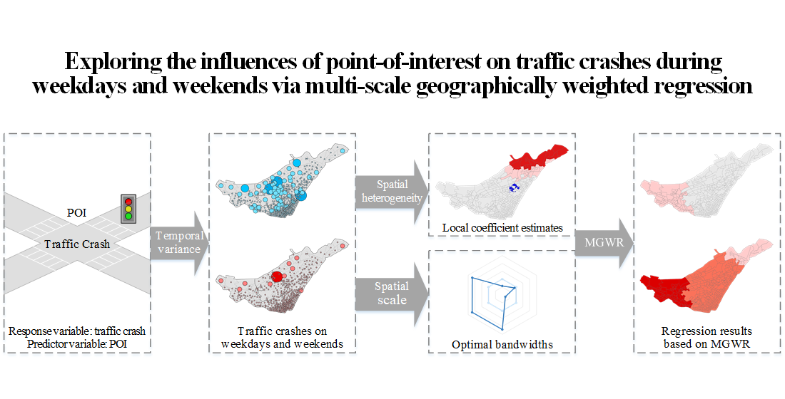
Exploring the Influences of Point-of-Interest on Traffic Crashes during Weekdays and Weekends via Multi-Scale Geographically Weighted Regression

 ,
,
Abstract
:
1. Introduction
1.1. Background
1.2. Related Work
1.3. Objectives of the Study
2. Study Area and Data Source
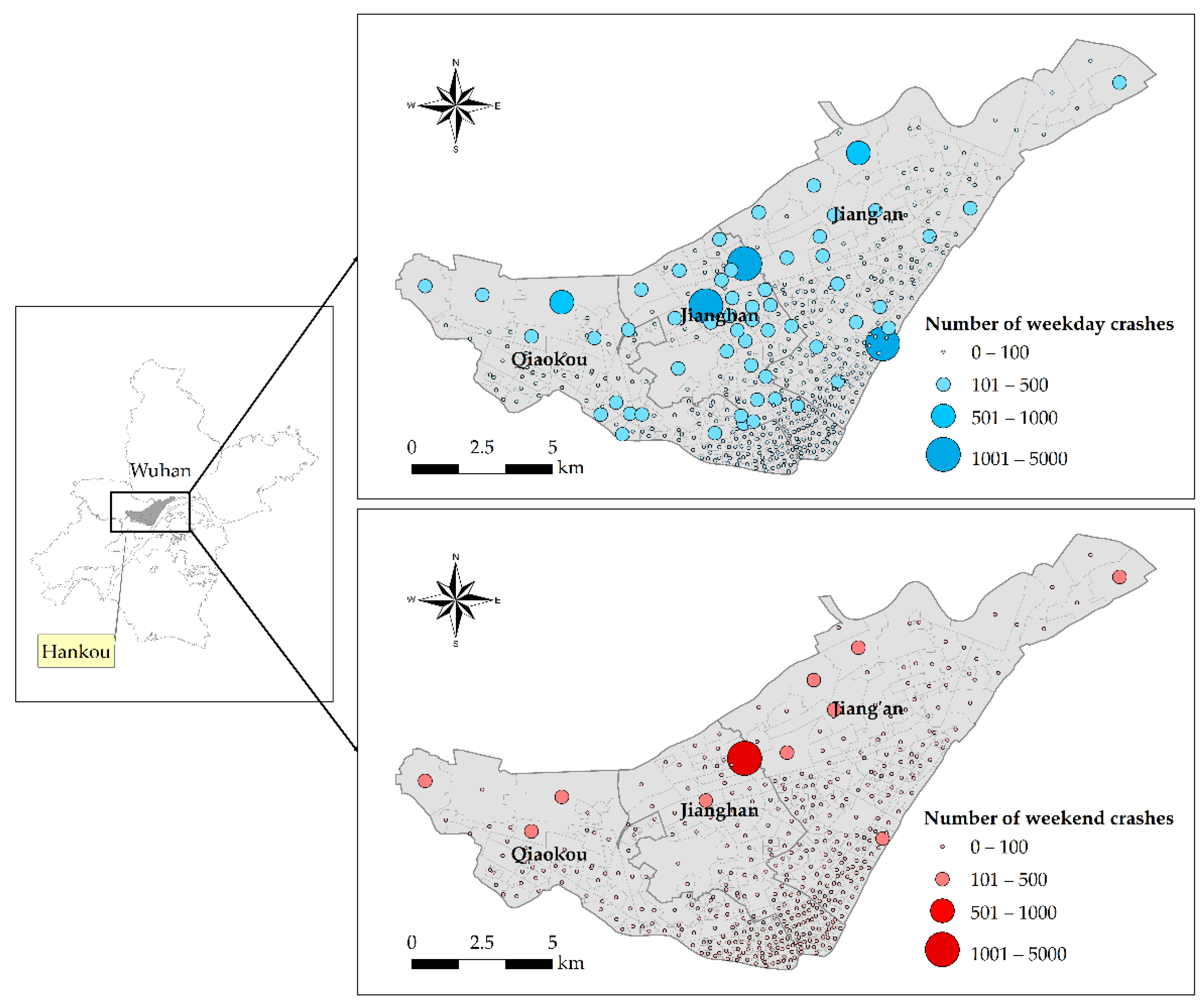
2.1. Study Area
2.2. Data Source
3. Methodology
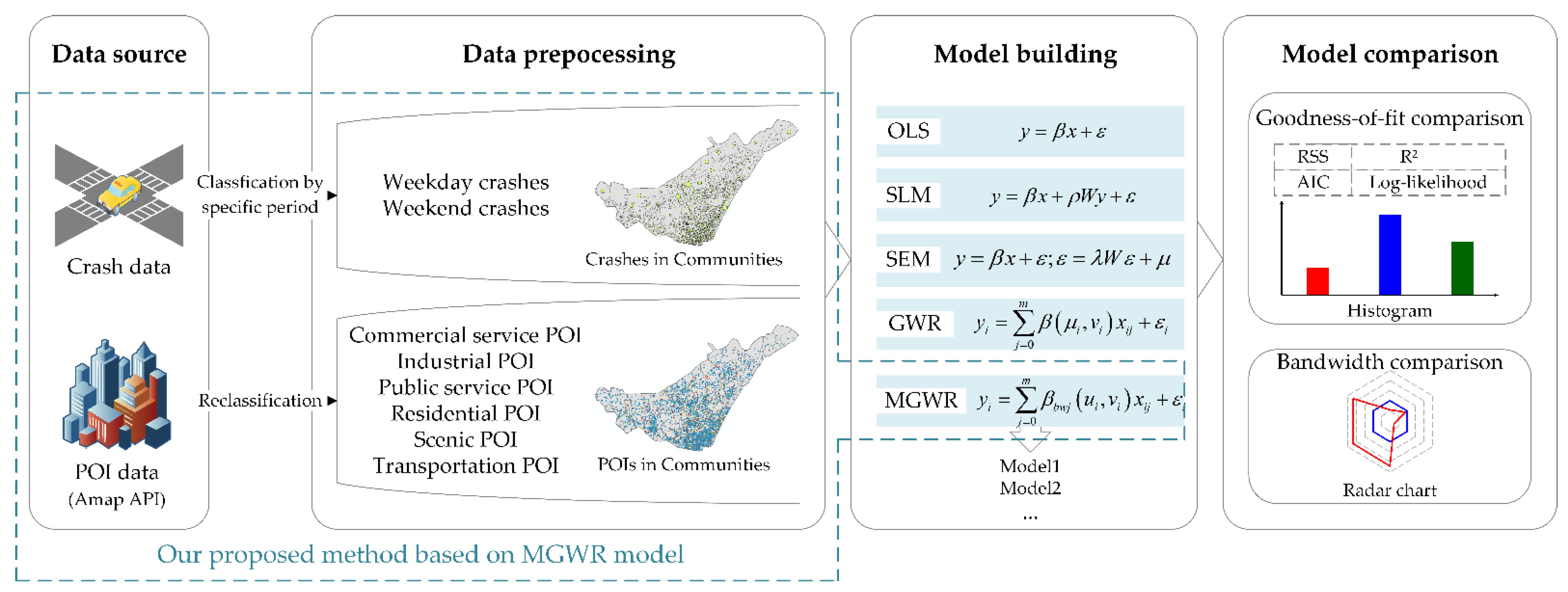
3.1. Data Pre-Processing
3.2. Regression Models
3.2.1. Global Regression Models
Ordinary Least Squares
Spatial Lag Model and Spatial Error Model
3.2.2. Local Regression Models
Geographically Weighted Regression
Multi-Scale Geographically Weighted Regression
3.3. Method Comparison
4. Results and Discussion
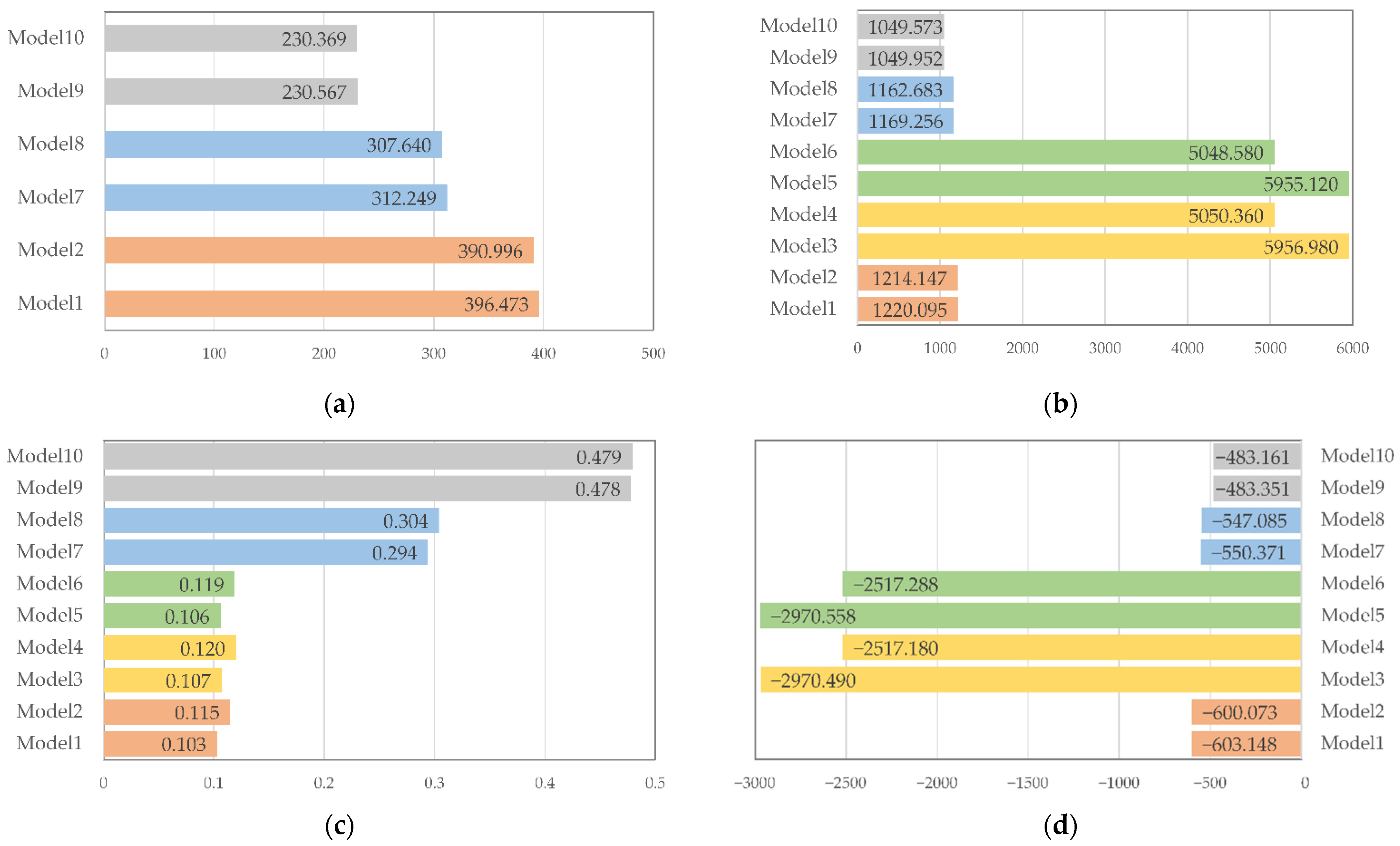
4.1. Model Comparison
4.2. Results from the Proposed Method Based on MGWR
4.3. Discussion
5. Conclusions
Author Contributions
Funding
Institutional Review Board Statement
Informed Consent Statement
Data Availability Statement
Acknowledgments
Conflicts of Interest
Abbreviations
| MGWR | Multiscale geographically weighted regression [25] |
| POI | Point-of-interest |
| OLS | Ordinary least squares [41] |
| SLM | Spatial lag model [42] |
| SEM | Spatial error model [42] |
| GWR | Geographically weighted regression [13] |
| VIF | Variance inflation factor |
| AIC | Akaike information criterion [45] |
| AICc | Corrected Akaike information criterion [45,46] |
| GAM | Generalized additive model [48] |
| RSS | Residual sum of squares |
References
- World Health Organization. World Health Statistics 2020: Monitoring Health for the SDGs, Sustainable Development Goals; World Health Organization: Geneva, Switzerland, 2020; ISBN 978-92-4-000510-5. [Google Scholar]
- Pulugurtha, S.S.; Duddu, V.R.; Kotagiri, Y. Traffic Analysis Zone Level Crash Estimation Models Based on Land Use Characteristics. Accid. Anal. Prev. 2013, 50, 678–687. [Google Scholar] [CrossRef] [PubMed]
- Xu, C.; Wang, Y.; Ding, W.; Liu, P. Modeling the Spatial Effects of Land-Use Patterns on Traffic Safety Using Geographically Weighted Poisson Regression. Netw. Spat. Econ. 2020, 20, 1015–1028. [Google Scholar] [CrossRef]
- Levine, N.; Kim, K.E.; Nitz, L.H. Spatial Analysis of Honolulu Motor Vehicle Crashes: I. Spatial Patterns. Accid. Anal. Prev. 1995, 27, 663–674. [Google Scholar] [CrossRef]
- Ukkusuri, S.; Miranda-Moreno, L.F.; Ramadurai, G.; Isa-Tavarez, J. The Role of Built Environment on Pedestrian Crash Frequency. Saf. Sci. 2012, 50, 1141–1151. [Google Scholar] [CrossRef]
- Kim, K.; Pant, P.; Yamashita, E. Accidents and Accessibility: Measuring Influences of Demographic and Land Use Variables in Honolulu, Hawaii. Transp. Res. Rec. 2010, 2147, 9–17. [Google Scholar] [CrossRef]
- Xie, B.; An, Z.; Zheng, Y.; Li, Z. Incorporating Transportation Safety into Land Use Planning: Pre-Assessment of Land Use Conversion Effects on Severe Crashes in Urban China. Appl. Geogr. 2019, 103, 1–11. [Google Scholar] [CrossRef]
- Miranda-Moreno, L.F.; Morency, P.; El-Geneidy, A.M. The Link between Built Environment, Pedestrian Activity and Pedestrian–Vehicle Collision Occurrence at Signalized Intersections. Accid. Anal. Prev. 2011, 43, 1624–1634. [Google Scholar] [CrossRef] [PubMed]
- Hadayeghi, A.; Shalaby, A.; Persaud, B. Development of Planning-Level Transportation Safety Models Using Full Bayesian Semiparametric Additive Techniques. J. Transp. Saf. Secur. 2010, 2, 45–68. [Google Scholar] [CrossRef]
- Narayanamoorthy, S.; Paleti, R.; Bhat, C.R. On Accommodating Spatial Dependence in Bicycle and Pedestrian Injury Counts by Severity Level. Transp. Res. Part B Methodol. 2013, 55, 245–264. [Google Scholar] [CrossRef] [Green Version]
- Kim, K.; Yamashita, E. Motor Vehicle Crashes and Land Use: Empirical Analysis from Hawaii. Transp. Res. Rec. 2002, 1784, 73–79. [Google Scholar] [CrossRef]
- Jia, R.; Khadka, A.; Kim, I. Traffic Crash Analysis with Point-of-Interest Spatial Clustering. Accid. Anal. Prev. 2018, 121, 223–230. [Google Scholar] [CrossRef]
- Stewart Fotheringham, A.; Charlton, M.; Brunsdon, C. The Geography of Parameter Space: An Investigation of Spatial Non-Stationarity. Int. J. Geogr. Inf. Syst. 1996, 10, 605–627. [Google Scholar] [CrossRef]
- Erdogan, S. Explorative Spatial Analysis of Traffic Accident Statistics and Road Mortality among the Provinces of Turkey. J. Saf. Res. 2009, 40, 341–351. [Google Scholar] [CrossRef]
- Rhee, K.-A.; Kim, J.-K.; Lee, Y.; Ulfarsson, G.F. Spatial Regression Analysis of Traffic Crashes in Seoul. Accid. Anal. Prev. 2016, 91, 190–199. [Google Scholar] [CrossRef]
- Li, Z.; Wang, W.; Liu, P.; Bigham, J.M.; Ragland, D.R. Using Geographically Weighted Poisson Regression for County-Level Crash Modeling in California. Saf. Sci. 2013, 58, 89–97. [Google Scholar] [CrossRef]
- Pirdavani, A.; Bellemans, T.; Brijs, T.; Wets, G. Application of Geographically Weighted Regression Technique in Spatial Analysis of Fatal and Injury Crashes. J. Transp. Eng. 2014, 140, 04014032. [Google Scholar] [CrossRef]
- Shariat-Mohaymany, A.; Shahri, M.; Mirbagheri, B.; Matkan, A.A. Exploring Spatial Non-Stationarity and Varying Relationships between Crash Data and Related Factors Using Geographically Weighted Poisson Regression: Non-Stationarity and Varying Relationships between Crash Data and Related Factors. Trans. GIS 2015, 19, 321–337. [Google Scholar] [CrossRef]
- Hezaveh, A.M.; Arvin, R.; Cherry, C.R. A Geographically Weighted Regression to Estimate the Comprehensive Cost of Traffic Crashes at a Zonal Level. Accid. Anal. Prev. 2019, 131, 15–24. [Google Scholar] [CrossRef]
- Gomes, M.J.T.L.; Cunto, F.; da Silva, A.R. Geographically Weighted Negative Binomial Regression Applied to Zonal Level Safety Performance Models. Accid. Anal. Prev. 2017, 106, 254–261. [Google Scholar] [CrossRef]
- Liu, J.; Khattak, A.J.; Wali, B. Do Safety Performance Functions Used for Predicting Crash Frequency Vary across Space? Applying Geographically Weighted Regressions to Account for Spatial Heterogeneity. Accid. Anal. Prev. 2017, 109, 132–142. [Google Scholar] [CrossRef]
- Obelheiro, M.R.; da Silva, A.R.; Nodari, C.T.; Cybis, H.B.B.; Lindau, L.A. A New Zone System to Analyze the Spatial Relationships between the Built Environment and Traffic Safety. J. Transp. Geogr. 2020, 84, 102699. [Google Scholar] [CrossRef]
- Wang, C.; Li, S.; Shan, J. Non-Stationary Modeling of Microlevel Road-Curve Crash Frequency with Geographically Weighted Regression. ISPRS Int. J. Geo-Inf. 2021, 10, 286. [Google Scholar] [CrossRef]
- Tang, J.; Gao, F.; Liu, F.; Han, C.; Lee, J. Spatial Heterogeneity Analysis of Macro-Level Crashes Using Geographically Weighted Poisson Quantile Regression. Accid. Anal. Prev. 2020, 148, 105833. [Google Scholar] [CrossRef]
- Fotheringham, A.S.; Yang, W.; Kang, W. Multiscale Geographically Weighted Regression (MGWR). Ann. Am. Assoc. Geogr. 2017, 107, 1247–1265. [Google Scholar] [CrossRef]
- Mollalo, A.; Vahedi, B.; Rivera, K.M. GIS-Based Spatial Modeling of COVID-19 Incidence Rate in the Continental United States. Sci. Total Environ. 2020, 728, 138884. [Google Scholar] [CrossRef]
- Maiti, A.; Zhang, Q.; Sannigrahi, S.; Pramanik, S.; Chakraborti, S.; Cerda, A.; Pilla, F. Exploring Spatiotemporal Effects of the Driving Factors on COVID-19 Incidences in the Contiguous United States. Sustain. Cities Soc. 2021, 68, 102784. [Google Scholar] [CrossRef] [PubMed]
- Mansour, S.; Al Kindi, A.; Al-Said, A.; Al-Said, A.; Atkinson, P. Sociodemographic Determinants of COVID-19 Incidence Rates in Oman: Geospatial Modelling Using Multiscale Geographically Weighted Regression (MGWR). Sustain. Cities Soc. 2021, 65, 102627. [Google Scholar] [CrossRef]
- Wu, C.; Ren, F.; Hu, W.; Du, Q. Multiscale Geographically and Temporally Weighted Regression: Exploring the Spatiotemporal Determinants of Housing Prices. Int. J. Geogr. Inf. Sci. 2019, 33, 489–511. [Google Scholar] [CrossRef]
- Tomal, M. Exploring the Meso-Determinants of Apartment Prices in Polish Counties Using Spatial Autoregressive Multiscale Geographically Weighted Regression. Appl. Econ. Lett. 2021, 1–9. [Google Scholar] [CrossRef]
- Fotheringham, A.S.; Yue, H.; Li, Z. Examining the Influences of Air Quality in China’s Cities Using Multi-scale Geographically Weighted Regression. Trans. GIS 2019, 23, 1444–1464. [Google Scholar] [CrossRef]
- Fan, Z.; Zhan, Q.; Yang, C.; Liu, H.; Zhan, M. How Did Distribution Patterns of Particulate Matter Air Pollution (PM 2.5 and PM 10) Change in China during the COVID-19 Outbreak: A Spatiotemporal Investigation at Chinese City-Level. Int. J. Environ. Res. Public Health 2020, 17, 6274. [Google Scholar] [CrossRef]
- Yan, J.-W.; Tao, F.; Zhang, S.-Q.; Lin, S.; Zhou, T. Spatiotemporal Distribution Characteristics and Driving Forces of PM2.5 in Three Urban Agglomerations of the Yangtze River Economic Belt. Int. J. Environ. Res. Public Health 2021, 18, 2222. [Google Scholar] [CrossRef]
- Stewart Fotheringham, A.; Li, Z.; Wolf, L.J. Scale, Context, and Heterogeneity: A Spatial Analytical Perspective on the 2016 U.S. Presidential Election. Ann. Am. Assoc. Geogr. 2021, 1–20. [Google Scholar] [CrossRef]
- Zhang, L.; Cheng, J.; Jin, C.; Zhou, H. A Multiscale Flow-Focused Geographically Weighted Regression Modelling Approach and Its Application for Transport Flows on Expressways. Appl. Sci. 2019, 9, 4673. [Google Scholar] [CrossRef] [Green Version]
- Iyanda, A.E.; Osayomi, T. Is There a Relationship between Economic Indicators and Road Fatalities in Texas? A Multiscale Geographically Weighted Regression Analysis. GeoJournal 2021, 86, 2787–2807. [Google Scholar] [CrossRef]
- Erdogan, S.; Yilmaz, I.; Baybura, T.; Gullu, M. Geographical Information Systems Aided Traffic Accident Analysis System Case Study: City of Afyonkarahisar. Accid. Anal. Prev. 2008, 40, 174–181. [Google Scholar] [CrossRef] [PubMed]
- Yu, R.; Abdel-Aty, M. Investigating the Different Characteristics of Weekday and Weekend Crashes. J. Saf. Res. 2013, 46, 91–97. [Google Scholar] [CrossRef] [PubMed]
- Anowar, S.; Yasmin, S.; Tay, R. Comparison of Crashes during Public Holidays and Regular Weekends. Accid. Anal. Prev. 2013, 51, 93–97. [Google Scholar] [CrossRef]
- Yue, H.; Zhu, X.; Ye, X.; Guo, W. The Local Colocation Patterns of Crime and Land-Use Features in Wuhan, China. ISPRS Int. J. Geo-Inf. 2017, 6, 307. [Google Scholar] [CrossRef] [Green Version]
- Anselin, L.; Bera, A.K.; Florax, R.; Yoon, M.J. Simple Diagnostic Tests for Spatial Dependence. Reg. Sci. Urban Econ. 1996, 26, 77–104. [Google Scholar] [CrossRef]
- Anselin, L.; Rey, S. Properties of Tests for Spatial Dependence in Linear Regression Models. Geogr. Anal. 2010, 23, 112–131. [Google Scholar] [CrossRef]
- Pellegrini, P.A.; Fotheringham, A.S. Modelling Spatial Choice: A Review and Synthesis in a Migration Context. Prog. Hum. Geogr. 2002, 26, 487–510. [Google Scholar] [CrossRef]
- Murakami, D.; Lu, B.; Harris, P.; Brunsdon, C.; Charlton, M.; Nakaya, T.; Griffith, D.A. The Importance of Scale in Spatially Varying Coefficient Modeling. Ann. Am. Assoc. Geogr. 2019, 109, 50–70. [Google Scholar] [CrossRef]
- Akaike, H. Factor Analysis and AIC. In Selected Papers of Hirotugu Akaike; Springer: New York, NY, USA, 1987. [Google Scholar]
- Sugiura, N. Further Analysts of the Data by Akaike’s Information Criterion and the Finite Corrections: Further Analysts of the Data by Akaike’ s. Commun. Stat.-Theory Methods 1978, 7, 13–26. [Google Scholar] [CrossRef]
- Yang, W. An Extension of Geographically Weighted Regression with Flexible Bandwidths. Ph.D. Thesis, University of St Andrews, St Andrews, Scotland, UK, 2014. [Google Scholar]
- Hastie, T.; Tibshirani, R. Generalized Additive Models: Some Applications. J. Am. Stat. Assoc. 1987, 82, 371–386. [Google Scholar] [CrossRef]
- Buja, A.; Hastie, T.; Tibshirani, R. Linear Smoothers and Additive Models. Ann. Statist. 1989, 17, 453–510. [Google Scholar] [CrossRef]
- Wolf, L.J.; Oshan, T.M.; Fotheringham, A.S. Single and Multiscale Models of Process Spatial Heterogeneity: Single and Multiscale Models. Geogr. Anal. 2018, 50, 223–246. [Google Scholar] [CrossRef] [Green Version]
- Oshan, T.; Li, Z.; Kang, W.; Wolf, L.; Fotheringham, A. Mgwr: A Python Implementation of Multiscale Geographically Weighted Regression for Investigating Process Spatial Heterogeneity and Scale. ISPRS Int. J. Geo-Inf. 2019, 8, 269. [Google Scholar] [CrossRef] [Green Version]
- Anselin, L.; Syabri, I.; Kho, Y.A. GeoDa: An Introduction to Spatial Data Analysis. In Handbook of Applied Spatial Analysis; Springer: Berlin/Heidelberg, Germany, 2010. [Google Scholar]
- Wang, P.; Ren, H.; Zhu, X.; Fu, X.; Liu, H.; Hu, T. Spatiotemporal Characteristics and Factor Analysis of SARS-CoV-2 Infections among Healthcare Workers in Wuhan, China. J. Hosp. Infect. 2021, 110, 172–177. [Google Scholar] [CrossRef]
- Huang, Y.; Wang, X.; Patton, D. Examining Spatial Relationships between Crashes and the Built Environment: A Geographically Weighted Regression Approach. J. Transp. Geogr. 2018, 69, 221–233. [Google Scholar] [CrossRef]
- Priyantha Wedagama, D.M.; Bird, R.N.; Metcalfe, A.V. The Influence of Urban Land-Use on Non-Motorised Transport Casualties. Accid. Anal. Prev. 2006, 38, 1049–1057. [Google Scholar] [CrossRef] [PubMed]
- Adanu, E.K.; Hainen, A.; Jones, S. Latent Class Analysis of Factors That Influence Weekday and Weekend Single-Vehicle Crash Severities. Accid. Anal. Prev. 2018, 113, 187–192. [Google Scholar] [CrossRef] [PubMed]
- Song, L.; Li, Y.; Fan, W.; Liu, P. Mixed Logit Approach to Analyzing Pedestrian Injury Severity in Pedestrian-Vehicle Crashes in North Carolina: Considering Time-of-Day and Day-of-Week. Traffic Inj. Prev. 2021, 22, 524–529. [Google Scholar] [CrossRef] [PubMed]


| Category | Narrowed Category |
|---|---|
| Residential POI | Commercial house, residential area |
| Commercial service POI | Tea house; bakery, coffee house, fast food restaurant, ice cream shop, dessert house, foreign food restaurant, leisure food restaurant, Chinese food restaurant, convenience store, supermarket, clothing store, personal care items shop, plants and pet market, home electronics hypermarket, home building materials market, shopping plaza, commercial street, sports store, stationery store, franchise store, comprehensive market, hotel, hostel, insurance company, finance company, finance and insurance service institution, bank, securities company, ATM, sports and recreation places, recreation place, theatre, cinema, recreation center |
| Industrial POI | Factory, company, enterprises, farming, forestry, animal husbandry and fishery base, industrial park |
| Transportation POI | Subway station, port, marina, bus station, railway station, ferry station, parking lot, coach station |
| Scenic POI | Scenery spot, park, square |
| Public service POI | Training institution, museum, archives hall, driving school, science and technology museum, science and education cultural place, research institution, art gallery, library, cultural palace, school, exhibition hall, hospital, special hospital, emergency center, disease prevention institution, industrial and commercial taxation institution, public security organization, traffic vehicle management, social group, governmental organization, social groups, holiday and nursing resort, sports stadium |
| Variables | Mean | Std. Dev. | Min. | Max. | VIF | |
|---|---|---|---|---|---|---|
| Response variables | Number of crashes on weekdays | 63.08 | 212.46 | 0 | 3877 | - |
| Number of crashes on weekends | 23.36 | 76.74 | 0 | 1365 | - | |
| Predictor variables | Number of commercial service POI | 191.89 | 247.91 | 0 | 2409 | 1.56 |
| Number of industrial POI | 30.72 | 55.47 | 0 | 450 | 2.47 | |
| Number of public service POI | 26.39 | 25.22 | 0 | 158 | 3.11 | |
| Number of residential POI | 9.12 | 8.79 | 0 | 64 | 2.02 | |
| Number of scenic POI | 1.31 | 8.58 | 0 | 167 | 1.19 | |
| Number of transportation POI | 15.59 | 18.86 | 0 | 136 | 4.03 | |
| Models | Description of the Models |
|---|---|
| Model 1 | The global regression model of POI and weekday crashes based on the OLS method. |
| Model 2 | The global regression model of POI and weekend crashes based on the OLS method. |
| Model 3 | The global regression model of POI and weekday crashes based on the SLM model. |
| Model 4 | The global regression model of POI and weekend crashes based on the SLM model. |
| Model 5 | The global regression model of POI and weekday crashes based on the SEM model. |
| Model 6 | The global regression model of POI and weekend crashes based on the SEM model. |
| Model 7 | The local regression model of POI and weekday crashes based on the GWR method. |
| Model 8 | The local regression model of POI and weekend crashes based on the GWR method. |
| Model 9 | The local regression model of POI and weekday crashes based on the MGWR method. |
| Model 10 | The local regression model of POI and weekend crashes based on the MGWR method. |
| Models | Evaluate Indexes | ||||
|---|---|---|---|---|---|
| RSS | AIC | R2 | Log-Likelihood | ||
| OLS | Model 1 | 396.473 | 1220.095 | 0.103 | −603.148 |
| Model 2 | 390.996 | 1214.147 | 0.115 | −600.073 | |
| SLM | Model 3 | - | 5956.980 | 0.107 | −2970.490 |
| Model 4 | - | 5050.360 | 0.120 | −2517.180 | |
| SEM | Model 5 | - | 5955.120 | 0.106 | −2970.558 |
| Model 6 | - | 5048.580 | 0.119 | −2517.288 | |
| GWR | Model 7 | 312.249 | 1169.256 | 0.294 | −550.371 |
| Model 8 | 307.640 | 1162.683 | 0.304 | −547.085 | |
| MGWR | Model 9 | 230.567 | 1049.952 | 0.478 | −483.351 |
| Model 10 | 230.369 | 1049.573 | 0.479 | −483.161 | |
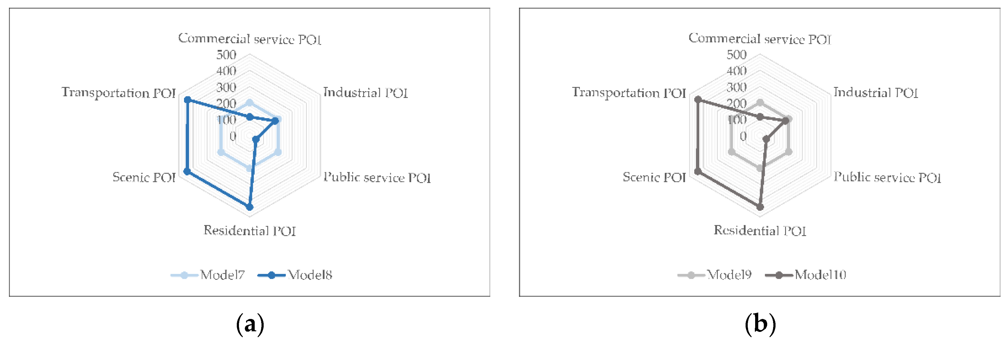
| Predictor Variables | Bandwidths | |||
|---|---|---|---|---|
| Model 7 | Model 8 | Model 9 | Model 10 | |
| Intercept | - | - | 442.000 | 442.000 |
| Commercial service POI | 202.000 | 202.000 | 114.000 | 114.000 |
| Industrial POI | 202.000 | 202.000 | 179.000 | 179.000 |
| Public service POI | 202.000 | 202.000 | 45.000 | 45.000 |
| Residential POI | 202.000 | 202.000 | 439.000 | 439.000 |
| Scenic POI | 202.000 | 202.000 | 441.000 | 441.000 |
| Transportation POI | 202.000 | 202.000 | 439.000 | 439.000 |
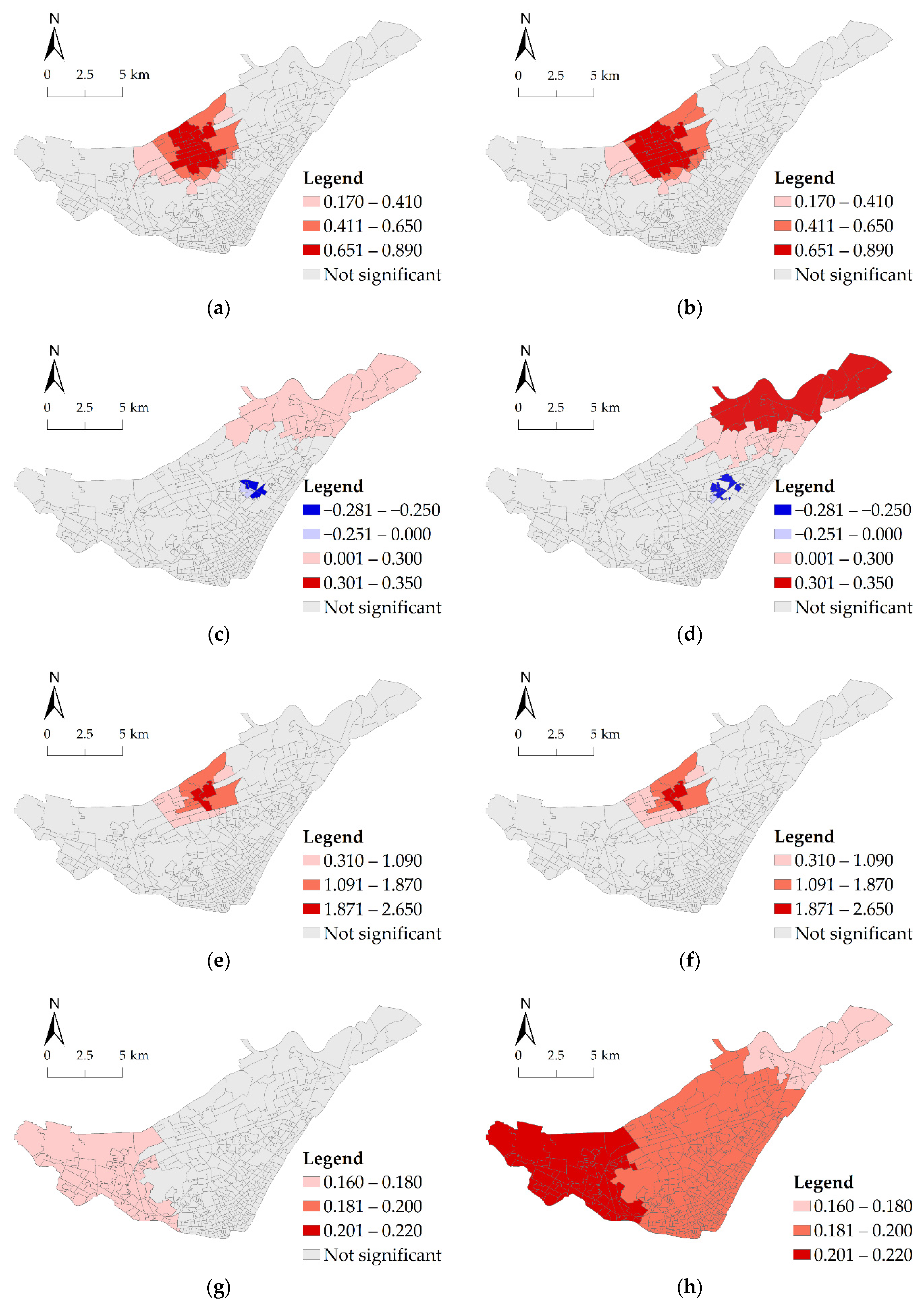
| Predictor Variables | Model 9 | Model 10 | ||||||||||
|---|---|---|---|---|---|---|---|---|---|---|---|---|
| MGWR Coefficients | Percentage of Communities by Significance (95% Level) of t-Test | MGWR Coefficients | Percentage of Communities by Significance (95% Level) of t-Test | |||||||||
| Mean | Min | Max | p ≤ 0.05 (%) | + (%) | − (%) | Mean | Min | Max | p ≤ 0.05 (%) | + (%) | − (%) | |
| Intercept | −0.044 | −0.067 | 0.022 | 0 | 0 | 0 | −0046 | −0.072 | 0.027 | 0 | 0 | 0 |
| Commercial service POI | 0.094 | −0.044 | 0.863 | 10.86 | 100 | 0 | 0.116 | −0.032 | 0.881 | 11.09 | 100 | 0 |
| Industrial POI | −0.013 | −0.269 | 0.293 | 7.24 | 81.25 | 18.75 | −0.025 | −0.281 | 0.347 | 9.95 | 75 | 25 |
| Public service POI | 0.093 | −0.253 | 2.644 | 5.66 | 100 | 0 | 0.079 | −0.268 | 2.533 | 5.43 | 100 | 0 |
| Residential POI | −0.046 | −0.062 | −0.041 | 0 | 0 | 0 | −0.047 | −0.062 | −0.042 | 0 | 0 | 0 |
| Scenic POI | 0.081 | 0.075 | 0.087 | 0 | 0 | 0 | 0.072 | 0.067 | 0.079 | 0 | 0 | 0 |
| Transportation POI | 0.162 | 0.144 | 0.179 | 15.16 | 100 | 0 | 0.192 | 0.177 | 0.212 | 100 | 100 | 0 |
Publisher’s Note: MDPI stays neutral with regard to jurisdictional claims in published maps and institutional affiliations. |
© 2021 by the authors. Licensee MDPI, Basel, Switzerland. This article is an open access article distributed under the terms and conditions of the Creative Commons Attribution (CC BY) license (https://creativecommons.org/licenses/by/4.0/).
Share and Cite
Qu, X.; Zhu, X.; Xiao, X.; Wu, H.; Guo, B.; Li, D. Exploring the Influences of Point-of-Interest on Traffic Crashes during Weekdays and Weekends via Multi-Scale Geographically Weighted Regression. ISPRS Int. J. Geo-Inf. 2021, 10, 791. https://0-doi-org.brum.beds.ac.uk/10.3390/ijgi10110791
Qu X, Zhu X, Xiao X, Wu H, Guo B, Li D. Exploring the Influences of Point-of-Interest on Traffic Crashes during Weekdays and Weekends via Multi-Scale Geographically Weighted Regression. ISPRS International Journal of Geo-Information. 2021; 10(11):791. https://0-doi-org.brum.beds.ac.uk/10.3390/ijgi10110791
Chicago/Turabian StyleQu, Xinyu, Xinyan Zhu, Xiongwu Xiao, Huayi Wu, Bingxuan Guo, and Deren Li. 2021. "Exploring the Influences of Point-of-Interest on Traffic Crashes during Weekdays and Weekends via Multi-Scale Geographically Weighted Regression" ISPRS International Journal of Geo-Information 10, no. 11: 791. https://0-doi-org.brum.beds.ac.uk/10.3390/ijgi10110791