
Revising Cadastral Data on Land Boundaries Using Deep Learning in Image-Based Mapping


Faculty of Civil and Geodetic Engineering, University of Ljubljana, Jamova Cesta 2, 1000 Ljubljana, Slovenia
*
Author to whom correspondence should be addressed.
ISPRS Int. J. Geo-Inf. 2022, 11(5), 298; https://0-doi-org.brum.beds.ac.uk/10.3390/ijgi11050298
Submission received: 3 March 2022
/
Revised: 21 April 2022
/
Accepted: 30 April 2022
/
Published: 4 May 2022
(This article belongs to the Special Issue Upscaling AI Solutions for Large Scale Mapping Applications)
Abstract
:One of the main concerns of land administration in developed countries is to keep the cadastral system up to date. The goal of this research was to develop an approach to detect visible land boundaries and revise existing cadastral data using deep learning. The convolutional neural network (CNN), based on a modified architecture, was trained using the Berkeley segmentation data set 500 (BSDS500) available online. This dataset is known for edge and boundary detection. The model was tested in two rural areas in Slovenia. The results were evaluated using recall, precision, and the F1 score—as a more appropriate method for unbalanced classes. In terms of detection quality, balanced recall and precision resulted in F1 scores of 0.60 and 0.54 for Ponova vas and Odranci, respectively. With lower recall (completeness), the model was able to predict the boundaries with a precision (correctness) of 0.71 and 0.61. When the cadastral data were revised, the low values were interpreted to mean that the lower the recall, the greater the need to update the existing cadastral data. In the case of Ponova vas, the recall value was less than 0.1, which means that the boundaries did not overlap. In Odranci, 21% of the predicted and cadastral boundaries overlapped. Since the direction of the lines was not a problem, the low recall value (0.21) was mainly due to overly fragmented plots. Overall, the automatic methods are faster (once the model is trained) but less accurate than the manual methods. For a rapid revision of existing cadastral boundaries, an automatic approach is certainly desirable for many national mapping and cadastral agencies, especially in developed countries.
1. Introduction
Mapping the boundaries of land rights, creating a complete cadastre and being able to keep it up to date is a major concern for land administration. Considering that three-quarters of the world’s land rights are not recognised and registered, it is necessary to speed up the process of cadastral mapping [1]. The challenge of creating a complete cadastre usually arises in developing countries—with low cadastral coverage [2,3]. Mapping and registering land rights in a formal cadastre is supposed to increase land tenure security [4,5]. However, an effective cadastre should also provide up-to-date information on people and land relationships beyond the adjudication stage [6,7]. Updating, in most cases, refers to the comparison of two datasets—one reflecting the state of the cadastral database and one newly acquired [8]. In view of this, the term “revision” is used as a synonym—since “updating” (as an act of formal change) is based on “revisions”.
In countries that already have a complete cadastre, providing up-to-date land data is a top priority [9]. It has taken decades for the cadastre to be complete in these countries, where conventional techniques such as ground-based surveying techniques or analogue aerial photogrammetry have typically been used [10]. Both methods are considered labour intensive and time-consuming [11,12]. The result was the creation of analogue cadastral maps and land records that later had to be digitised and integrated into a geographic information system (GIS) or broader land information systems. Although complete cadastres were created, many national mapping and cadastral agencies (NMCAs) failed to properly maintain the cadastres [13]. The reality that cadastres attempt to depict is complex and dynamic [14,15], and underestimating the dynamics of the relationships between people and land, in reality, has led to outdated cadastral maps. Apart from the advances in surveying and mapping technologies, most of which have already been tested in developing countries [16,17,18,19], cadastral surveying and boundary data maintenance in developed countries continued to be carried out using ground-based techniques such as tacheometry and global navigation satellite systems (GNSS) methods [10,12]. This approach presents many challenges in terms of mapping efficiency, which can be overcome by low-cost and rapid cadastral surveying and indirect mapping techniques.
Indirect mapping techniques rely on delineating visible cadastral boundaries from high-resolution remote sensing imagery. The application of image-based cadastral mapping is based on the recognition that many cadastral boundaries coincide with natural or man-made structures that are readily visible on remote sensing imagery [3,17]. In cadastral applications, unmanned aerial vehicles (UAVs) have shown great potential for mapping land parcel boundaries in both rural and urban areas [18,20,21,22]. In addition, UAV-based orthoimagery has been considered as a basemap for the creation of cadastral maps and for the revision of existing cadastral maps [23,24,25]. Apart from the high visibility of spatial units on UAV imagery relevant to cadastral mapping, many previous case studies have reported the manual delineation of spatial units [16], but only a limited number of studies have investigated the automatic mapping approach. The innovative approaches aim to simplify and speed up image-based cadastral mapping by automating the delineation of visible boundaries. Mainly, customised image segmentation and edge detection algorithms have been used to automatically adjust cadastral mapping [23,26].
Modern methods for automatic boundary detection in cadastral mapping also include deep learning [27,28,29,30]. Recent studies indicate that deep learning such as convolutional neural networks (CNNs) ensure a higher accuracy in delineating visible land boundaries than some of the state-of-the-art machine learning or object-based techniques [27,28]. CNNs can be trained in two ways: from scratch or by transfer learning [31]. When training the model from scratch, remote sensing data have to be provided, i.e., images and labels. In transfer learning, the model is pre-trained, usually with a large amount of data with more abstract features, and the last convolutional layer is trained with the specific features of the new application. Crommelinck et al. [27] pre-trained the model using transfer-learning and reported that VGG19, i.e., 19 layers deep CNN, provides a more automated and accurate detection of visible boundaries from UAV imagery than random forest. The pre-training was based on aerial imagery, which also had to be provided. Furthermore, the study highlights that the model based on VGG19 provides more promising metrics than some other architectures (such as ResNet, MobileNet, and DenseNet). Xia et al. [28] investigated a fully CNN for cadastral boundary detection in urban and semi-urban areas. The model was trained from scratch using UAV tiles, and the results show that the approach outperformed object-based techniques, including global probability boundary (gPb) and multi-resolution segmentation (MRS). Park and Song [32] aimed to detect the changes between existing cadastral maps and current land use boundaries in the field. The model was trained from scratch using hyperspectral UAV imagery. However, providing thousands of UAV training data can be considered a limitation, especially when a model is trained from scratch, as highlighted in [29]. This can be overcome with a CNN architecture that requires less training data, for instance, U-Net, followed by data augmentation prior to processing [29,33]. The challenge here remains to confirm what should be a sufficient variety of UAV training data to learn a robust network model.
Objective of the Study
In general, it is argued that the main challenge with CNNs supporting cadastral mapping is the processing of a large amount of remote sensing training data and the computational requirements. Therefore, an important condition for any deep learning method is that the total time required to detect the final boundaries, including pre- and post-processing, should not be longer than the total time of a manual method [10]. This serves as a justification and allows the objective of this study to be defined.
The main objective of this study was to develop an efficient and cost-effective approach for mapping visible land boundaries using CNN. The mapping approach is based on the detection of visible land boundaries that coincide with large parts of the cadastral boundaries—especially in rural areas. Automation of visible land boundary detection can be used to revise existing cadastral maps and to automatically identify areas where updates are needed. At this point, it should be emphasised that not all cadastral boundaries are visible and that some of them are difficult to detect on UAV imagery.
2. Materials and Methods
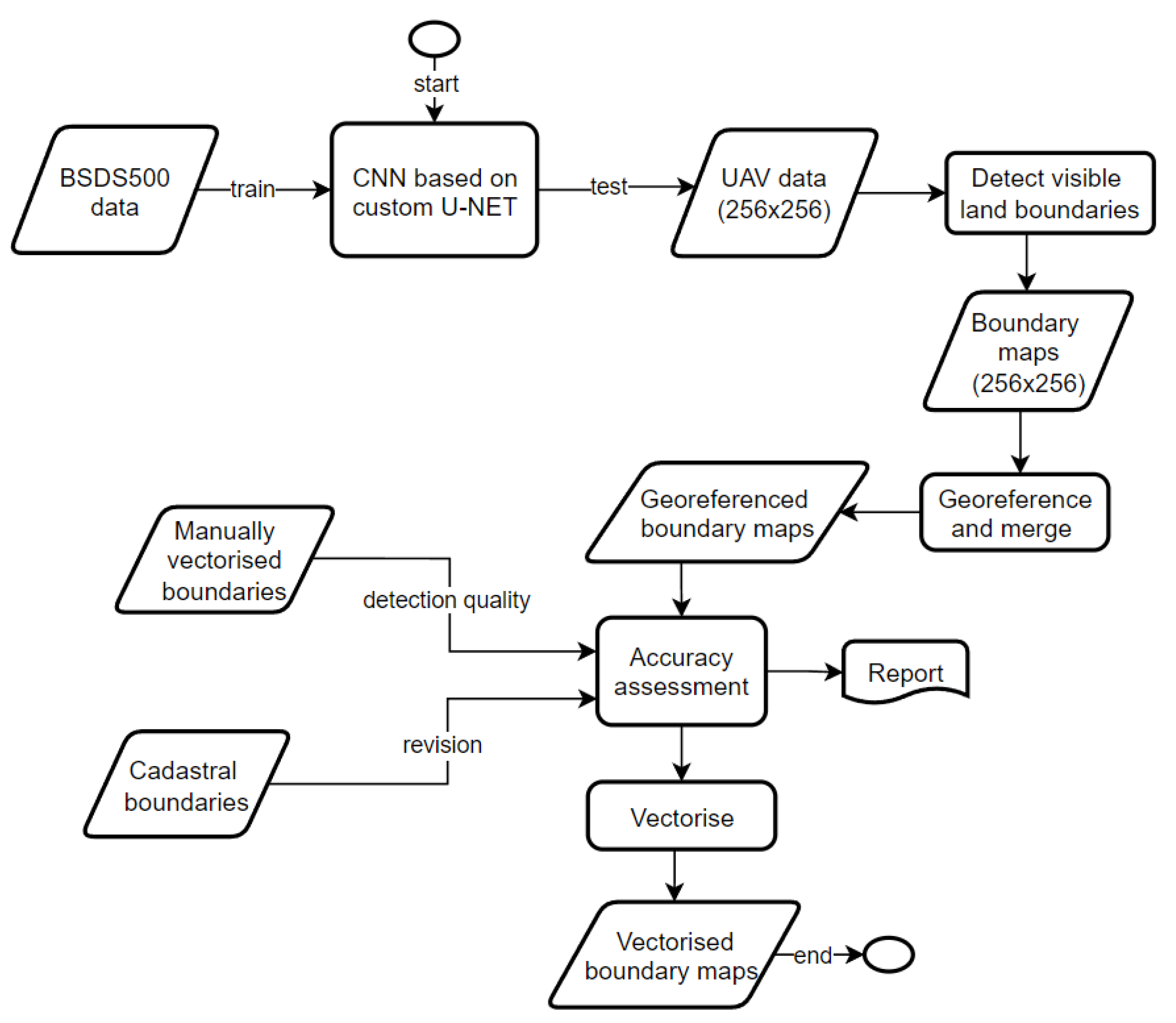
The workflow of this study was comprised of four core parts, i.e., the training approach, visible boundary detection, accuracy assessment, and vectorisation of boundary maps. The individual steps and details are described in the following subsections. The generalised workflow is shown in Figure 1.
2.1. Training Approach and Dataset
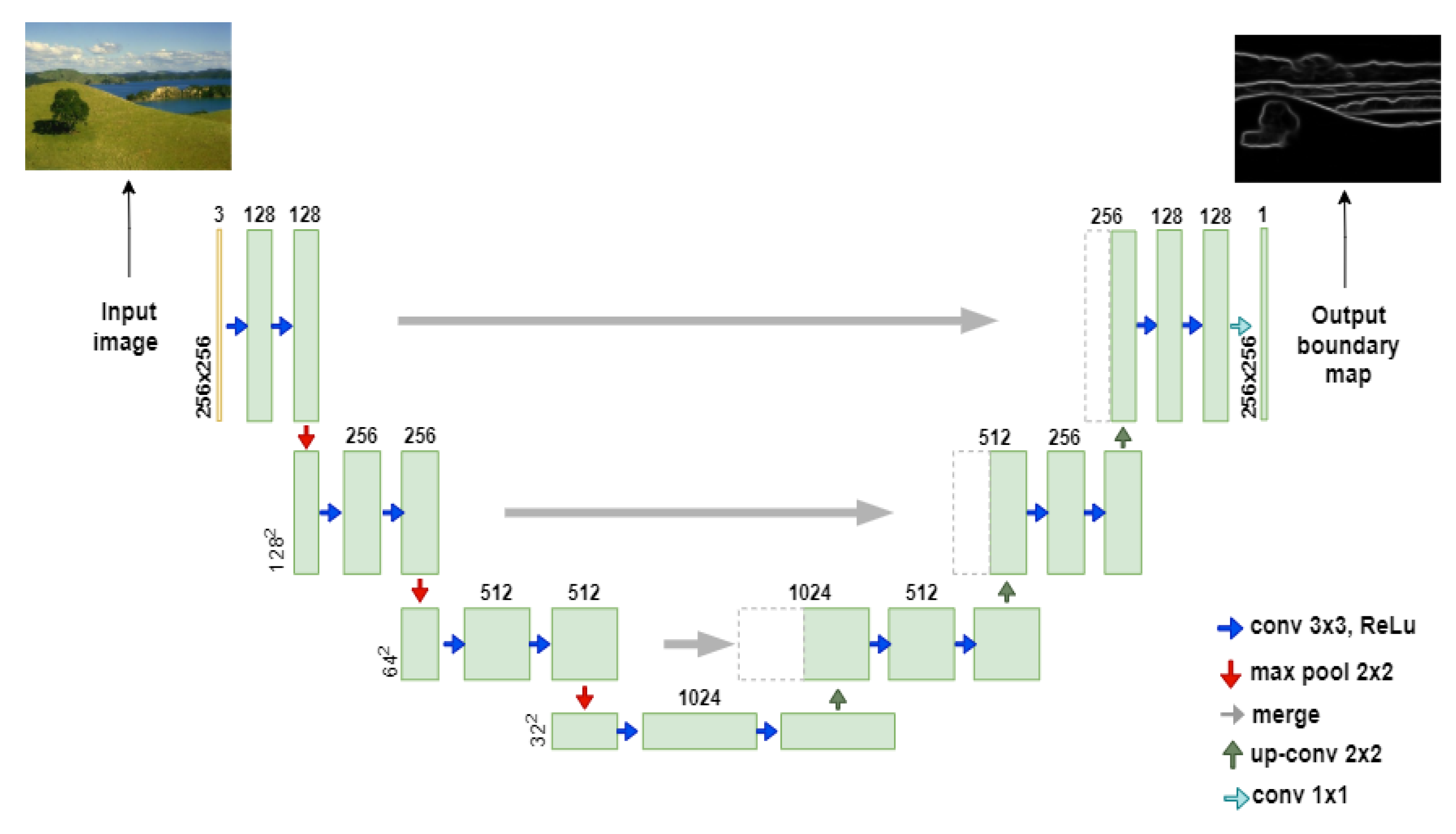
Considering the main objective, a CNN that requires a smaller amount of training data is preferable. U-Net is a CNN architecture that provides fast and precise localisation of features from images. The U-Net consists of an encoding path and a decoding path, giving it a U-shape. The encoding path is a convolutional network consisting of repeated convolutions (3 × 3), each followed by a ReLU and max-pooling (2 × 2) operation. During the encoding path, spatial resolution is decreased while feature information is increased. The decoding path combines spatial and feature information through a sequence of up-convolutions (2 × 2) and merging with high-resolution features from the decoding path, where the size of the images is converted to their original size. A detailed description of the original U-Net architecture can be found in [33]. In this study, the U-Net was considered as a deep learning-based detector for visible boundaries.
Given the complexity of our domain problem, namely the detection of visible land boundaries to revise existing cadastral maps, the original architecture was customised and is shown in Figure 2. The customisation included the removal of the first level of the original U-Net. This reduces the number of parameters that can be trained and was sufficient in terms of complexity for our domain problem.
The model was trained using the Berkeley segmentation data set 500 (BSDS500) and is available at [34]. BSDS500 is an accessible dataset and a standard benchmark for image segmentation and edge or boundary detection tasks that can be used to train the CNN while matching the domain problem of this study. The dataset consists of 500 everyday images and their corresponding labels. The approach is intended to be transferable to images of other scenes and contexts—for example, UAV images. The data is organised in training, validation, and test subsets. Each image has hand-labelled boundaries that come from an average of five annotators, or about 2500 samples in total. To increase the number of training samples and to improve the flexibility of the validation split, the images of the training and validation subsets were merged into one. In addition, the target image size was set to 256 × 256 pixels.
Training a CNN requires a lot of memory and a powerful graphics processing unit (GPU) to perform efficient computations. To combat this, the training of the customised U-Net with the BSDS500 dataset was performed in Google Collaboratory [35]. The model was implemented in Keras [36], and the process was written in Python using the TensorFlow library [37]. The trained model was tested using UAV images with a size of 256 × 256 pixels.
2.2. Visible Boundary Detection from UAV Data
Two rural areas were selected to test the U-Net model, one in Ponova vas and the other in Odranci, both in Slovenia. The rural areas were chosen because the number of visible cadastral boundaries in these areas is higher than in dense urban areas.
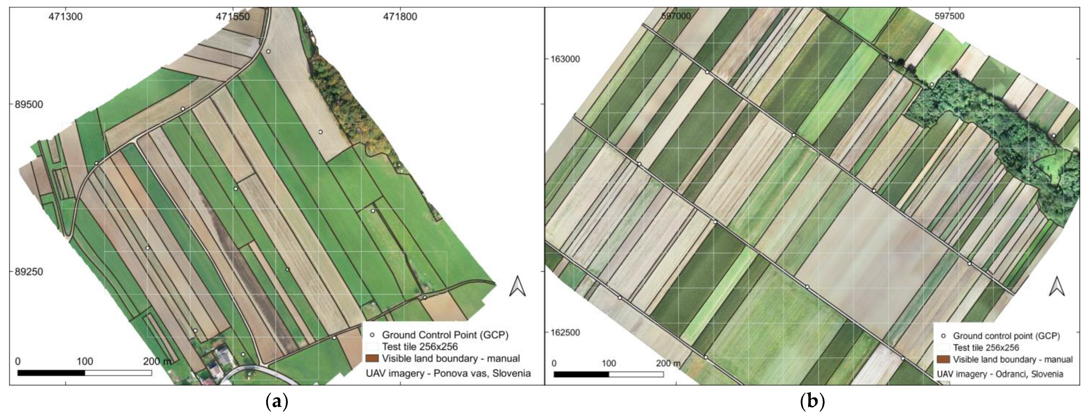
In Ponova vas, the flight altitude was set to 80 m, and 354 images were acquired to cover the study area (Figure 3a). The UAV images were indirectly georeferenced using 12 ground control points (GCPs) evenly distributed over the field. The GCPs were surveyed with real-time kinematic (RTK) using the global navigation satellite system (GNSS) and Leica Viva receiver. The study area had an area of 25 ha, and an orthoimage with ground sampling distance (GSD) of 2.0 cm was produced from UAV images.
In Odranci, UAV images were acquired at the altitude of 90 m, and 997 images were acquired to cover the study area (Figure 3b). A total of 18 GCPs were used to georeference the UAV images. The GCPs were surveyed using RTK with the Leica GS18 GNSS receiver. The GSD of the produced orthoimage was 2.3 cm, and the study area had an area of 63.9 ha.
All UAV data were acquired using a rotary-wing drone, the DJI Phantom 4 Pro. The selected rural areas included agricultural fields, roads, tree groves, and hedgerows. Table 1 shows the specifications of the UAV data.
UAV orthoimages for Ponova vas and Odranci were randomly tiled in 256 × 256 pixels. To increase the field of view for each tile, the original spatial resolution of the UAV orthoimages had to be converted to a larger GSD, from 2 cm to 25 cm, using the nearest neighbour resampling method. In addition, corresponding ground truth images (also called label images) were created for each UAV image. The 256 × 256 × 1 ground images were created from the manually digitised visible land boundaries, which were originally in the vector format (Figure 3a,b). Since the predicted boundary maps were in the raster format, the reference boundaries were buffered by 50 cm and later rasterised using tools from GRASS GIS [38]. Comparison of the predicted boundaries with the manually vectorised boundaries allowed the CNN model to be evaluated, i.e., the ability of the model to produce boundary maps for visible land boundaries.
In addition, cadastral boundaries were also used as reference data. The cadastral boundaries were rasterised using the same tool and buffer size as the manual boundaries. Unlike the manual approach, by comparing the predicted boundaries with the cadastral boundaries, the number of cadastral boundaries that overlap with the visible land boundaries can be determined. This approach allowed existing cadastral maps to be revised. The current cadastral boundaries were retrieved from the e-portal of the Slovenian NMCA, an online platform for requesting official cadastral data [39].
The predicted boundary maps were not georeferenced. Since georeferencing is a key component in cadastral mapping, further edits were made. First, the predicted boundary maps (for each UAV tile) were georeferenced. Second, the georeferenced tiles were merged to obtain the boundary map for the entire extent. The analysis and further processing were performed using GDAL [40], Rasterio [41], and Numpy [42]. After georeferencing, the merged boundary maps were used to evaluate the accuracy and to quantify the overlap between visible and cadastral boundaries.
2.3. Accuracy Assessment
The accuracy assessment refers to the evaluation of the CNN model and the evaluation of the detection quality of the visible land boundaries for the UAV data.
The CNN model, namely the customised U-Net model, was monitored with accuracy and loss during the training. The loss represents the difference between the boundaries predicted by the model and the reference boundaries. In this study, cross-entropy loss was used—the most common loss function used in CNNs. The performance of the model was measured using overall accuracy. Overall accuracy as an evaluation metric is defined as the sum of correctly predicted boundaries by the model divided by all predicted boundaries. The definitions and equations for cross-entropy and overall accuracy can be found in [43].
Boundary detection based on CNNs falls into the domain of binary classification. Here, it is a challenge to find balanced pixels for the classes “boundary” and “no boundary”. The reason is that the number of background pixels (class “no boundary”) in predicted boundary maps or cadastral maps is always much higher than the number of pixels representing the boundaries themselves. For this reason, detection quality (i.e., the degree of correctly detected visible boundaries compared to reference data) was evaluated by calculating the F1 score, recall, and precision—more appropriate metrics for unbalanced classes. In such a calculation, the “boundary” pixels were defined as a positive class since this was the focus of our study.
Table 2 shows the confusion matrix used to evaluate the detection quality of visible land boundaries and the overlap between visible and cadastral boundaries. The confusion matrix classifies pixels into true positive (TP), false positive (FP), true negative (TN), and false negative (FN).
Based on the number of pixels in the confusion matrix, recall and precision are calculated with the following equations:
Recall can be interpreted as completeness, while precision means correctness, and both are important for cadastral mapping. The F1 score is composed of recall and precision and is expressed by the following equation:
2.4. Vectorisation of Predicted Boundary Maps—Hough Transform
Current cadastral maps are in the vector format and are usually integrated into the GIS environment. To obtain cadastral compliant output data, an automatic vectorisation process was implemented. The predicted boundary maps were available in the raster format, with pixel values from 0 to 1—for each UAV tile as the input. Once georeferenced, the predicted boundaries were automatically vectorised using the Hough transform [44,45]. Vectorisations were performed for binary predicted maps, with a threshold “boundary” ≥0.3 and “boundary” ≥0.5. Thresholds were chosen based on an assessment of the accuracy of detected visible land boundaries.
The Hough transform extracts straight lines or curves from images and can be used for digitising cadastral maps [46], or for the extraction of land boundaries [47]. The feature extraction technique was implemented in Matlab. Here, the technique was designed to detect lines, using the parametric representation of a line:
where:
ρ—the distance from the origin to the line along a vector perpendicular to the line,
θ—the angle between the x-axis and this vector.
Various parameters for vectorisation were tested and empirically confirmed that the following parameters generally gave the best results: the resolution for ρ and θ was set to 2 and 0.05, respectively, and lines with a length of at least 10 pixels and filled gaps of 10 pixels between segments of a straight line were searched for. Vectorisation of relatively small tiles using Hough transform is not computationally demanding, which allowed us to implement it iteratively. After vectorising the straight line which corresponded to the highest value of Hough transform, the pixels in the binary image within a distance of 3 pixels from the vectorised line were set to 0. Then the Hough transformation was performed again. With the implemented method, the lines were simplified and avoided the vectorisation of doubly adjacent lines.
3. Results
3.1. CNN and Training Approach
Based on the custom U-Net architecture, the CNN was trained with the BSDS500 dataset, with the target size set to 256 × 256 pixels. The training images were in RGB, and 30% of the training data was used for validation. This resulted in 1505 samples for training and 645 samples for validation.
After some testing, the training parameters were adjusted to fine-tune the model. To avoid changing the size of the predicted boundary maps for each input image, a max-pooling method with equal padding was specified. In addition, a dropout rate of 0.5 was used. The dropout rate is used to ignore randomly selected neurons to avoid overfitting the model. The layer depth was set to 1024, and a sigmoid was used as the final activation layer. During training, the Adam optimiser was used with a learning rate of 10−4.
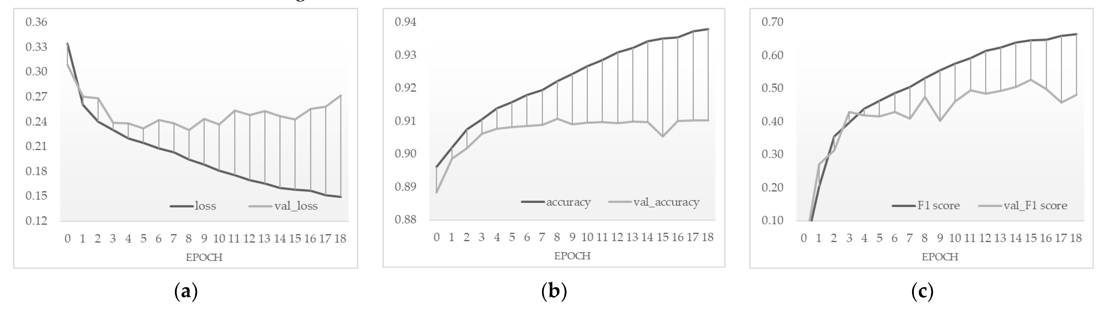
The model was trained with a batch size of 16 for 50 epochs. The early stop function with the patience of 10 epochs was activated. This feature stops training when the performance of the model in a validation dataset stops improving. The number of steps per epoch was calculated by dividing the total number of training samples by the batch size. Training was performed in Google Collaboratory. The service provides access to different GPUs that affect the training time. In this study, the service provided a GPU with 12.7 GB RAM. The early stop ended the training at epoch 18, which took 1.5 h. With a more powerful GPU, e.g., 25 GB, training the model for 100 epochs took 82 min (with a batch size of 32 and without early stop). The training performance of the adapted U-Net is shown in Figure 4.
3.2. Visible Boundary Detection from UAV Imageries
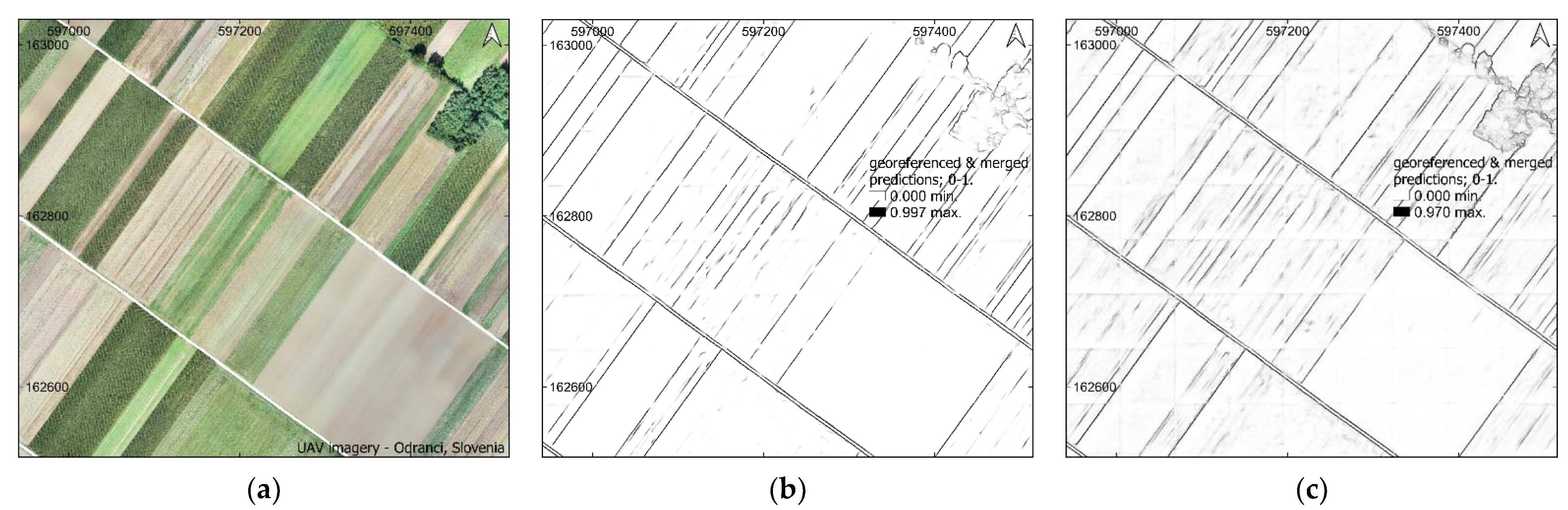
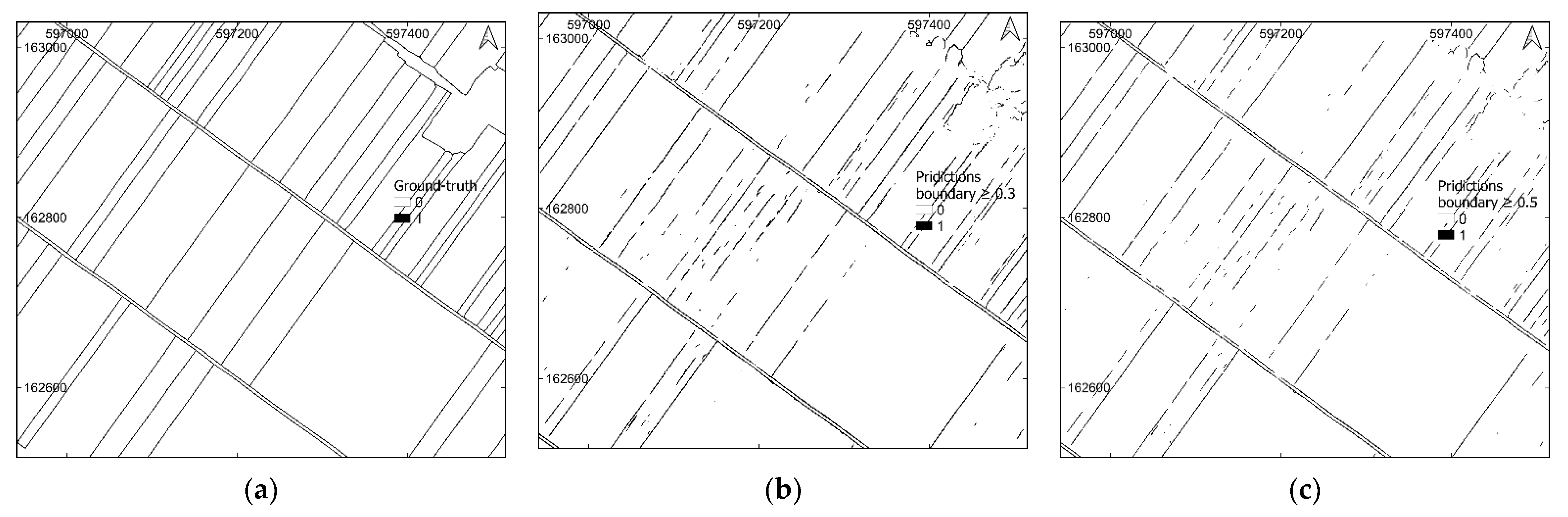
Once the model was trained, it was applied to 256 × 256 × 3 UAV images to detect visible land boundaries. A prediction boundary map was created for each UAV tile. The boundary maps were georeferenced and merged to determine the total extent of the test area. The results of the predicted boundary maps based on georeferenced and merged UAV tiles are shown in Figure 5 and Figure 6. In addition, the results obtained with the customised CNN were compared with the original U-Net.
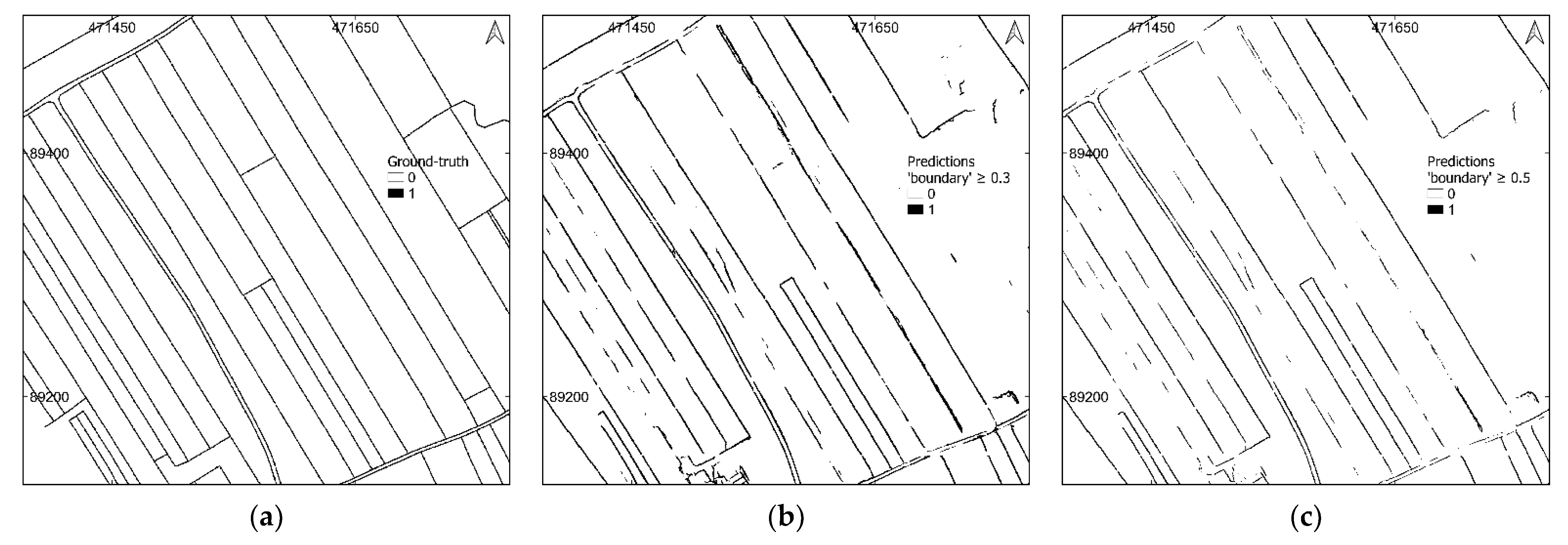
The predicted boundary maps, shown in Figure 5 and Figure 6, had pixel values ranging from 0 to 1. To evaluate the detection quality of the visible land boundaries, the predictions were compared to the ground truth data on land boundaries that had been manually digitised from the UAV imagery. The ground data consisted of two classes, i.e., “boundary” and “no boundary” with values of 1 and 0, respectively, so the predicted boundary maps were reclassified into two classes with threshold values of 0.3 and 0.5. The results of the reclassified boundary maps are shown in Figure 7 and Figure 8.
3.3. Revision of Existing Cadatral Data on Land Boundaries
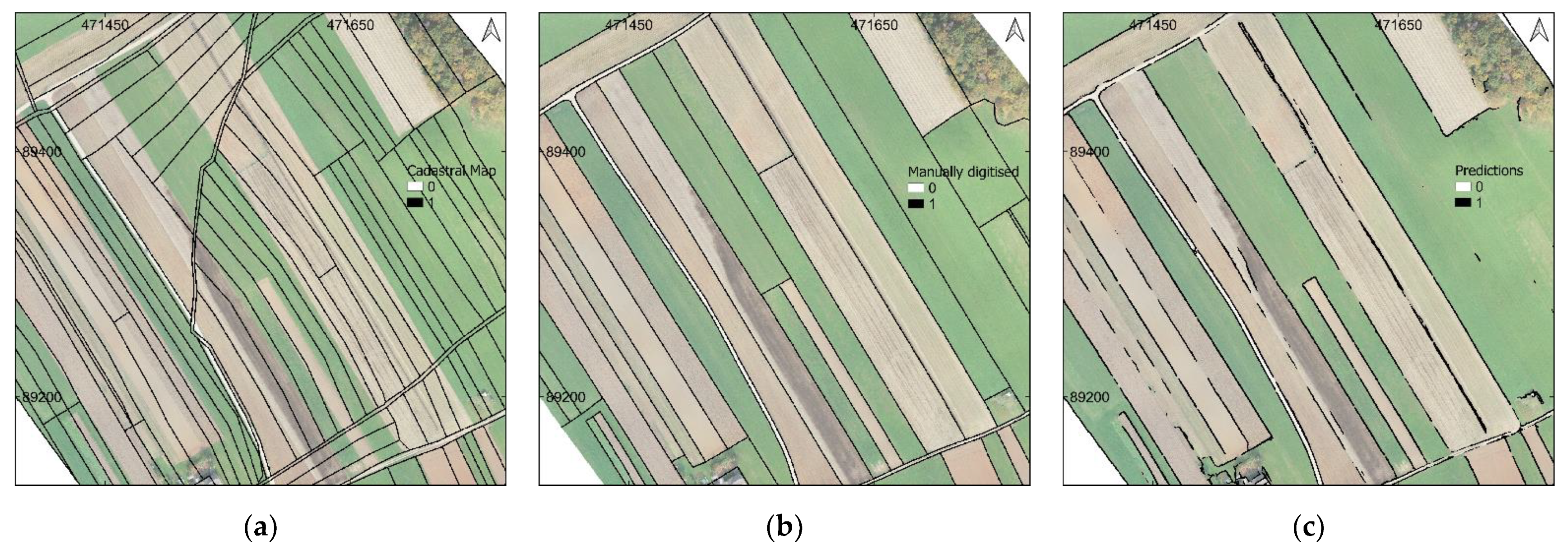
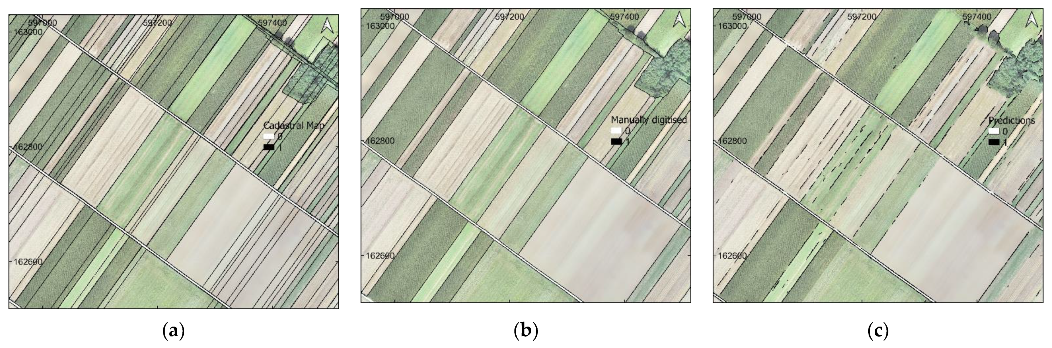
The predicted land boundary maps with the highest F1 score, obtained with customised CNN (Table 3 and Table 4), were used to further revise the existing cadastral maps for the two test areas, Ponova vas and Odranci. In addition, the manually vectorised visible boundaries were compared with the existing cadastral data on land boundaries to obtain reference values for the overlap of the two geospatial data layers. The revision of the existing cadastral maps was based on the same metrics used to evaluate accuracy in the previous section. The existing cadastral maps were compared to the automatically detected visible boundaries, as shown in Figure 9 and Figure 10. The accuracy assessment is shown in Table 5 and Table 6.
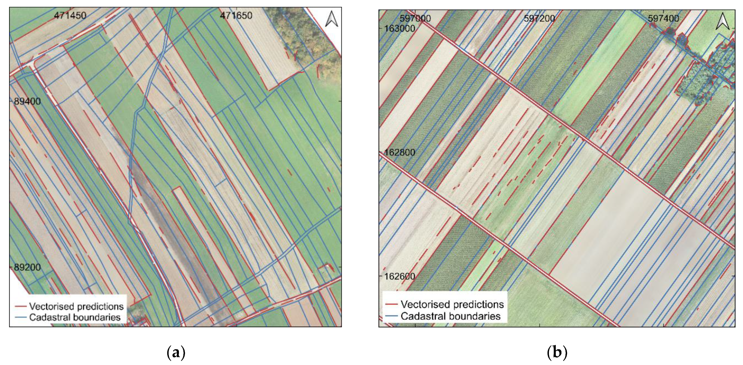
The predicted boundaries were vectorised to match the format of the current cadastral data. Vectorisation was performed using the Hough transform. The fill gap of 10 was applied because it was considered more appropriate, and we thus avoided the possibility of bias in the predicted boundaries. This approach not only vectorised the pixels defined as the “boundary” but also produced straight lines, which are crucial for cadastral mapping. This can be considered a vectorisation and simplification step. Once the vectorisation was complete, we also created an overlapping (discrepancy) map, which can be seen in Figure 11.
4. Discussion
The discussion is divided into three parts: (i) CNN and training approach for visible land boundary mapping; (ii) detection of visible land boundaries using UAV imagery and deep learning and (iii) revision of existing cadastral maps based on the detected and digitised visible land boundaries, addressing the objectives of our study.
4.1. CNN and Training Approach
In general, deep learning is a relatively new research area in the geospatial domain and offers great potential for feature recognition from remote sensing imagery [30]. The upscaling deep learning solutions, including CNNs, for visible land boundary detection is becoming increasingly important, especially for UAV-based cadastral mapping [27,29]. Deep learning requires processing a large amount of training data and powerful computations. In this study, an efficient and cost-effective deep learning approach was developed that provides reasonable results and helps to further automate the cadastral mapping process.
The CNN model is based on the U-Net architecture [33]. Since our research problem was binary classification, the original U-Net architecture was simplified (Figure 2) to reduce the number of training parameters and training time. This led to a more efficient and, at the same time, more accurate result compared to the original architecture (Figure 5 and Figure 6 and Table 3 and Table 4).
Training of the CNN model was based on the BSDS500 dataset [34]. This dataset is well known for edge or boundary detection tasks and already fitted the purpose of the study. The CNN model was trained from scratch, and no additional preparation of the training data was completed since the dataset contained both images and labels. Typically, CNNs are trained from scratch or by transfer learning. Both approaches require the preparation of custom training data, including images and labels, which usually takes some time and has already been highlighted in [27,28,29]. However, the amount of training data depends on the type of CNN architecture used. For example, the U-Net is an architecture that requires less training data and still provides accurate localisations [33]. In this study, the model was trained with 1505 samples, which can be considered a small amount of training data, but the model still provided satisfactory results. In addition, the model was trained for 18 epochs and required a total of 1.5 h to complete the training, which can also be considered a fast approach. The CNN model was trained in Google Collaboratory [35]. This approach reduces the cost of strong GPUs and RAM and can be considered a low-cost approach. The only bottleneck is the provided RAM memory, which varies from 12.7 GB to 25 GB. These variations also affect the training time. In addition, there were some interruptions during the training, so a local computer is beneficial in this area and can be considered a more stable solution.
Model performance during training was monitored by loss, overall accuracy, and F1 score (Figure 4). The loss decreased steadily from the first epoch to the end of training. The early stop function monitored the validation loss to stop the training before the model was over-fitted. The overall accuracy had high values from the beginning of the training, mainly due to the unbalanced pixels for the “boundary” and “no boundary” classes. In addition, the F1 score was applied. At this point, it should be emphasised that the overall accuracy cannot be considered as a suitable metric to monitor the performance of the model during training. The reason is that the main problem in boundary detection tasks is the unbalanced number of pixels per class. Normally, the boundary pixels occupy a small number of pixels compared to the background pixels. For this reason, the model was additionally monitored with the F1 score, which was calculated only for pixels of the class “boundary”.
4.2. Visible Boundary Detection from UAV Imageries
In this study, deep learning was used as a detector for visible land boundaries. Once the model was trained, it was applied to the UAV test data. First, the original UAV or-thoimages were resampled from 2 cm to 25 cm GSD. This was performed to increase the field of view for each test UAV tile with a size of 256 × 256 pixels. A map of visible land boundaries was created for each tile. Second, the predicted boundary maps were georeferenced and later merged, as this is essential for cadastral mapping.
To evaluate the quality of the predicted boundary maps, they were compared with manually digitised boundaries from UAV orthoimagery. The evaluation was based on recall, precision, and F1 score, as this is considered a reasonable and unambiguous approach. Boundary maps were buffered (with 50 cm) and rasterised, and a value of 0 was set for the “no boundary” class and a value of 1 for the “boundary” class. The boundary maps generated by the CNN model originally ranged from 0 to 1. Therefore, the boundary maps were reclassified with a threshold value where “boundary” ≥ 0.3 and “boundary” ≥ 0.5.
Boundary maps with a threshold of 0.3 generated more balanced values for recall and precision (and at the same time a higher F1 score) compared to predictions with a threshold of 0.5 (Table 3 and Table 4). For Ponova vas, we obtained an F1 score of 0.60 for a threshold of 0.3 and an F1 score of 0.55 for a threshold of 0.5. In the case of Odranci, the results showed an F1 score of 0.54 and 0.51 for a threshold of 0.3 and 0.5, respectively. It is worth highlighting here that the higher the threshold for the “boundary” class, the higher the precision and the lower the recall. For cadastral mapping, both values can be considered relevant since recall represents completeness (the number of detected boundaries compared to the reference data), while precision represents the correctness of the detected boundaries. Considering this, an F1 score as high as possible would have been desirable. The threshold can be used as an aid or balance between recall and precision and can be used depending on the purpose or requirement. In short, the higher the completeness or the detected boundaries, the lower the correctness and vice versa.
Boundary maps created using a customised CNN (basically a simplified U-Net) were additionally compared to a CNN based on the original U-net architecture [33]. This was used to evaluate our adapted approach. The results obtained with the original U-Net for both thresholded boundary maps showed worse results compared to our adapted model. The best results were obtained for reclassified boundary maps with a threshold of 0.3, namely an F1 score of 0.54 for Ponova vas and an F1 score of 0.49 for Odranci.
What would be a perfect F1 score for cadastral mapping is not easy to determine. First of all, not all cadastral boundaries are visible. Second, it depends on the area where the CNN model is tested and the scenes it covers, for example, rural, urban, or mixed. This is also true when comparing the results of one study to another, as methods and case studies differ, thus making reliable comparison impossible [27,28]. However, for further analyses, such as revising existing cadastral boundaries, an F1 score of 60 is considered sufficient for rapid analysis, especially in rural areas.
4.3. Revision of Existing Cadatral Data on Land Boundaries
Predicted visible land boundaries were compared with official data, i.e., cadastral boundaries, to revise current cadastral maps [39]. The cadastral boundaries were buffered and rasterised in the same manner as the manually delineated boundaries. The boundary maps that provided a higher F1 score were selected to revise the existing cadastral maps in Ponova vas and Odranci, both in Slovenia. The revision was based on the same metrics, namely recall, precision, and F1 score. Before comparing the predicted boundaries with the cadastral boundaries, reference values were generated by comparing the cadastral boundaries to the manually delineated visible land boundaries on the same UAV imagery (Table 5 and Table 6). This was undertaken because the manually digitised boundaries were assumed to have complete and correct data and were defined as ground truth data.
In the case of Ponova vas, it was obvious even from visual interpretation that the cadastral map was outdated (Figure 9a). The currently visible land boundaries (the boundaries that define the use of the land on site) did not match the cadastral boundaries. This was also confirmed by the accuracy assessment. The results presented in Table 5 showed very low values, namely a recall of 0.06, a precision of 0.10 and an F1 score of 0.07 compared to the predicted boundaries. Almost the same results were obtained when comparing with the ground truth data (recall: 0.05, precision: 0.09, F1 score: 0.07). In this case, very low metrics, specifically low recall, can be interpreted as an indicator of the identification of specific areas where cadastral updates are needed. In addition, the metrics generated when compared to the predictions also did not indicate any overlap between the visible and cadastral boundaries (regardless of the fact that not all visible boundaries were automatically generated). A very low recall indicates that there must also be a problem with the directions of the cadastral boundaries and that they do not correspond to the situation on the ground. In order to align the land possession and (legal) cadastral data, a complex revision of cadastral data is required in Ponova vas, using legal cadastral instruments, such as the setting up cadastral data or restructuring of land parcels through complex land consolidation. For these purposes, the provided data on visible land boundaries can serve as important input data, for creating or updating cadastral maps [16,20].
In the case of Odranci, the situation is a little different since the direction of the cadastral boundaries matched the direction of the visible land boundaries (Figure 10a). The results yielded a recall of 0.21, a precision of 0.49, and an F1 of 0.29, compared to reference values of 0.37, 0.63, and 0.47. From these metrics, 37% of the visible land boundaries overlapped with the cadastral boundaries, which corresponded to a correctness of 63% (based on ground truth data). Our CNN provided a lower F1 score, which was to be expected, but at the same time, it was sufficient to determine boundary overlaps [3]. The values of recall and precision indicated that the direction and location of the cadastral boundaries were consistent with the visible boundaries. The low values for overlap could be due to excessive fragmentation. Many parcels were fragmented into small pieces while they were shown under the same land cover in the UAV imagery. This was also evident from the visual interpretation. A simplified land consolidation merging land units would have been preferable in Odranci, where, again, the provided data on visible land boundaries can serve as important input data.
For both study areas, the predicted boundary maps were also vectorised using the Hough transform (Figure 11). In addition to vectorisation, the Hough transform provided straight lines and filled some gaps—this can also be considered a simplification approach. In this study, a filling gap of 10 was used so as not to bias the predicted results. Moreover, increasing the value for filling the gaps sometimes led to undesirable results. Vectorisation is crucial for cadastral mapping because it allows for further analysis. In this study, the evaluation of accuracy was performed on a pixel basis. Further studies could focus on comparing pixel-based methods with object-based methods to evaluate accuracy, such as the buffer overlay method [48], once the predicted boundaries are vectorised. In the buffer overlay method, the buffer can be increased around the cadastral data, which is called a tolerance in cadastral applications; this may not affect the assessment of completeness because the approach is based on the length that falls within the buffer. In the pixel-based method, if the width or buffer of the reference data is increased while the predictions are thinner, this would lead to a bias in completeness and correctness.
5. Conclusions
In the last decade, much attention has been given to the creation of cadastral maps and the establishment of cadastral systems, including innovative surveying and mapping techniques, but less to the maintenance and sustainability of the cadastral systems. This article focused on data maintenance by revising existing cadastral maps using deep learning. The whole workflow was developed and presented, starting with training the CNN, detecting the visible land boundaries, georeferencing, evaluating the model and vectorising the predicted boundary maps, and revising the existing cadastral maps. The model was tested with UAV imagery, but the developed approach could also be used for satellite or aerial imagery.
The approach can be considered efficient and cost-effective in automatically identifying areas where updates of cadastral maps are needed. In addition, the identified visible land boundaries could be used as input data for updating cadastral data or other cadastral procedures that can be applied for cadastral mapping, including for land parcel restructuring. The identified visible land boundaries did not represent final cadastral boundaries. They can be considered as preliminary boundaries for quick analysis and public presentations of the current state of the art.
One of the main land administration problems in developed countries is to keep the cadastral system up to date. Here, an automated approach that identifies the areas where such updates are needed would highlight and narrow down this challenge for NMCAs. Overall, it can be said that automatic methods are faster but less accurate (once the model is trained), while manual methods provide slower but more accurate boundary delineations. Combining automatic methods with manual corrections can reduce the user effort and still provide high accuracy. However, when revising existing cadastral boundaries, an automatic approach is certainly desirable for many NMCAs. It should also be reiterated that not all cadastral boundaries are visible in remote sensing imagery and not all can be automatically detected or extracted. Therefore, automating invisible cadastral boundaries by tagging them prior to UAV or satellite imagery acquisition could be an interesting and challenging task for further research.
Author Contributions
Conceptualisation, Bujar Fetai and Anka Lisec; methodology, Bujar Fetai; software, Bujar Fetai and Dejan Grigillo; validation, Bujar Fetai, Dejan Grigillo and Anka Lisec; formal analysis, Bujar Fetai and Anka Lisec; investigation, Bujar Fetai; resources, Bujar Fetai and Anka Lisec; data curation, Bujar Fetai and Anka Lisec; writing—original draft preparation, Bujar Fetai; writing—review and editing, Bujar Fetai, Dejan Grigillo and Anka Lisec; visualisation, Bujar Fetai; supervision, Anka Lisec. All authors have read and agreed to the published version of the manuscript.
Funding
This research and APC were funded by the Slovenian Research Agency (research core funding Earth observation and geoinformatics grant number P2-0406) and by the Slovenian Research Agency and Surveying and Mapping Authority of the Republic of Slovenia (research project grant number V2-1934).
Institutional Review Board Statement
Not applicable.
Informed Consent Statement
Not applicable.
Data Availability Statement
The data presented in this study are openly available in link (https://unilj-my.sharepoint.com/:f:/g/personal/bfetai_fgg_uni-lj_si/ErN_s1uLnidMmdyGk2ZPk8oBKEyFDzbT7wQ6PpS2yr9k-Q?e=mnxPJO, accessed on 2 March 2022); the training data in [34]; and official cadastral data in [39].
Acknowledgments
This research is part of the Ph.D. thesis of the corresponding author. We thank the anonymous reviewers for their insightful comments and suggestions. We acknowledge Klemen Kozmus Trajkovski for capturing the UAV data and Matej Račič for the technical support.
Conflicts of Interest
The authors declare no conflict of interest. The funders had no role in the design of the study; in the collection, analyses, or interpretation of data; in the writing of the manuscript, or in the decision to publish the results.
References
- Enemark, S.; Bell, K.C.; Lemmen, C.; McLaren, R. Fit-For-Purpose Land Administration: Joint FIG/World Bank Publication; FIG: Copenhagen, Denmark, 2014; ISBN 978-87-92853-10-3/978-87-92853-11-0. [Google Scholar]
- Williamson, I.P. Land Administration for Sustainable Development, 1st ed.; ESRI Press Academic: Redlands, CA, USA, 2010; ISBN 9781589480414. [Google Scholar]
- Luo, X.; Bennett, R.; Koeva, M.; Lemmen, C.; Quadros, N. Quantifying the Overlap between Cadastral and Visual Boundaries: A Case Study from Vanuatu. Urban Sci. 2017, 1, 32. [Google Scholar] [CrossRef] [Green Version]
- Enemark, S. Land Administration and Cadastral Systems in support of Sustainable Land Governance: A global approach. In Proceedings of the 3rd Land Administration Forum for the Asia and Pacific Region, Tehran, Iran, 24–26 May 2009; pp. 53–71. [Google Scholar]
- Simbizi, M.C.D.; Bennett, R.M.; Zevenbergen, J. Land tenure security: Revisiting and refining the concept for Sub-Saharan Africa’s rural poor. Land Use Policy 2014, 36, 231–238. [Google Scholar] [CrossRef]
- Grant, D.; Enemark, S.; Zevenbergen, J.; Mitchell, D.; McCamley, G. The Cadastral triangular model. Land Use Policy 2020, 97, 104758. [Google Scholar] [CrossRef]
- Enemark, S.; McLaren, R.; Lemmen, C. Fit-for-Purpose Land Administration—Providing Secure Land Rights at Scale. Land 2021, 10, 972. [Google Scholar] [CrossRef]
- Heipke, C.; Woodsford, P.A.; Gerke, M. Updating geospatial databases from images. In Advances in Photogrammetry, Remote Sensing and Spatial Information Sciences: 2008 ISPRS Congress Book; Baltsavias, E., Li, Z., Chen, J., Eds.; CRC Press: London, UK, 2008; ISBN 978-0-415-47805-2/978-0-203-88844-5. [Google Scholar]
- Kocur-Bera, K.; Frąszczak, H. Coherence of Cadastral Data in Land Management—A Case Study of Rural Areas in Poland. Land 2021, 10, 399. [Google Scholar] [CrossRef]
- Bennett, R.M.; Koeva, M.; Asiama, K. Review of Remote Sensing for Land Administration: Origins, Debates, and Selected Cases. Remote Sens. 2021, 13, 4198. [Google Scholar] [CrossRef]
- Koeva, M.; Stöcker, C.; Crommelinck, S.; Chipofya, M.; Kundert, K.; Schwering, A.; Sahib, J.; Zein, T.; Timm, C.; Humayun, M.; et al. Innovative Geospatial Solutions for Land Tenure Mapping. RJESTE 2020, 3, 34–49. [Google Scholar] [CrossRef]
- Stöcker, C.; Bennett, R.; Koeva, M.; Nex, F.; Zevenbergen, J. Scaling up UAVs for land administration: Towards the plateau of productivity. Land Use Policy 2022, 114, 105930. [Google Scholar] [CrossRef]
- Zevenbergen, J. Proceedings of the Land Administration: To See the Change from Day to Day: Inaugural Address by Jaap Zevenbergen, Professor of Land Administration Systems, Enschede, The Netherlands, 22 April 2009; ITC: Enschede, The Netherlands, 2009. ISBN 978-90-6164-274-9.
- Luo, X.; Bennett, R.M.; Koeva, M.; Lemmen, C. Investigating Semi-Automated Cadastral Boundaries Extraction from Airborne Laser Scanned Data. Land 2017, 6, 60. [Google Scholar] [CrossRef] [Green Version]
- Zevenbergen, J. A systems approach to land registration and cadastre. Nord. J. Surv. Real Estate Res. 2004, 1, 11–24. [Google Scholar]
- Crommelinck, S.; Bennett, R.; Gerke, M.; Nex, F.; Yang, M.; Vosselman, G. Review of Automatic Feature Extraction from High-Resolution Optical Sensor Data for UAV-Based Cadastral Mapping. Remote Sens. 2016, 8, 689. [Google Scholar] [CrossRef] [Green Version]
- Kohli, D.; Bennett, R.; Lemmen, C.; Morales, A.; Pinheiro, A.; Zevenbergen, J. A Quantitative Comparison of Completely Visible Cadastral Parcels Using Satellite Images: A Step towards Automation. In Proceedings of the FIG Working Week 2017, Helsinki, Finland, 29 May–2 June 2017; pp. 1–14. [Google Scholar]
- Ramadhani, S.A.; Bennett, R.M.; Nex, F.C. Exploring UAV in Indonesian cadastral boundary data acquisition. Earth Sci. Inform. 2018, 11, 129–146. [Google Scholar] [CrossRef]
- Casiano Flores, C.; Tan, E.; Crompvoets, J. Governance assessment of UAV implementation in Kenyan land administration system. Technology in Society 2021, 66, 101664. [Google Scholar] [CrossRef]
- Koeva, M.; Muneza, M.; Gevaert, C.; Gerke, M.; Nex, F. Using UAVs for map creation and updating. A case study in Rwanda. Surv. Rev. 2018, 50, 312–325. [Google Scholar] [CrossRef] [Green Version]
- Stöcker, C.; Nex, F.; Koeva, M.; Gerke, M. High-Quality UAV-Based Orthophotos for Cadastral Mapping: Guidance for Optimal Flight Configurations. Remote Sens. 2020, 12, 3625. [Google Scholar] [CrossRef]
- Rijsdijk, M.; van Hinsbergh, W.H.M.; Witteveen, W.; Buuren, G.H.M.; Schakelaar, G.A.; Poppinga, G.; van Persie, M.; Ladiges, R. Unmanned Aerial Systems in the process of Juridical verification of Cadastral borde. Int. Arch. Photogramm. Remote Sens. Spatial Inf. Sci. 2013, XL-1/W2, 325–331. [Google Scholar] [CrossRef] [Green Version]
- Crommelinck, S.; Bennett, R.; Gerke, M.; Yang, M.; Vosselman, G. Contour Detection for UAV-Based Cadastral Mapping. Remote Sens. 2017, 9, 171. [Google Scholar] [CrossRef] [Green Version]
- Puniach, E.; Bieda, A.; Ćwiąkała, P.; Kwartnik-Pruc, A.; Parzych, P. Use of Unmanned Aerial Vehicles (UAVs) for Updating Farmland Cadastral Data in Areas Subject to Landslides. IJGI 2018, 7, 331. [Google Scholar] [CrossRef] [Green Version]
- Manyoky, M.; Theiler, P.; Steudler, D.; Eisenbeiss, H. Unmanned Aerial Vehicle in Cadastral Applications. Int. Arch. Photogramm. Remote Sens. Spatial Inf. Sci. 2011, XXXVIII-1/C22, 57–62. [Google Scholar] [CrossRef] [Green Version]
- Wassie, Y.A.; Koeva, M.N.; Bennett, R.M.; Lemmen, C.H.J. A procedure for semi-automated cadastral boundary feature extraction from high-resolution satellite imagery. J. Spat. Sci. 2018, 63, 75–92. [Google Scholar] [CrossRef] [Green Version]
- Crommelinck, S.; Koeva, M.; Yang, M.Y.; Vosselman, G. Application of Deep Learning for Delineation of Visible Cadastral Boundaries from Remote Sensing Imagery. Remote Sens. 2019, 11, 2505. [Google Scholar] [CrossRef] [Green Version]
- Xia, X.; Persello, C.; Koeva, M. Deep Fully Convolutional Networks for Cadastral Boundary Detection from UAV Images. Remote Sens. 2019, 11, 1725. [Google Scholar] [CrossRef] [Green Version]
- Fetai, B.; Račič, M.; Lisec, A. Deep Learning for Detection of Visible Land Boundaries from UAV Imagery. Remote Sens. 2021, 13, 2077. [Google Scholar] [CrossRef]
- Ma, L.; Liu, Y.; Zhang, X.; Ye, Y.; Yin, G.; Johnson, B.A. Deep learning in remote sensing applications: A meta-analysis and review. ISPRS J. Photogramm. Remote Sens. 2019, 152, 166–177. [Google Scholar] [CrossRef]
- Garcia-Gasulla, D.; Parés, F.; Vilalta, A.; Moreno, J.; Ayguadé, E.; Labarta, J.; Cortés, U.; Suzumura, T. On the Behavior of Convolutional Nets for Feature Extraction. Jair 2018, 61, 563–592. [Google Scholar] [CrossRef] [Green Version]
- Park, S.; Song, A. Discrepancy Analysis for Detecting Candidate Parcels Requiring Update of Land Category in Cadastral Map Using Hyperspectral UAV Images: A Case Study in Jeonju, South Korea. Remote Sens. 2020, 12, 354. [Google Scholar] [CrossRef] [Green Version]
- Ronneberger, O.; Fischer, P.; Brox, T. U-Net: Convolutional Networks for Biomedical Image Segmentation. 2015. Available online: http://arxiv.org/pdf/1505.04597v1 (accessed on 22 February 2022).
- Arbeláez, P.; Fowlkes, C.; Martin, D. The Berkeley Segmentation Dataset and Benchmark. Available online: https://www2.eecs.berkeley.edu/Research/Projects/CS/vision/bsds/ (accessed on 2 March 2022).
- Google Colaboratory. Available online: https://colab.research.google.com (accessed on 6 December 2021).
- Chollet, F.; others. Keras. 2015. Available online: https://keras.io (accessed on 29 April 2021).
- Abadi, M.; Agarwal, A.; Barham, P.; Brevdo, E.; Chen, Z.; Citro, C.; Corrado, G.S.; Davis, A.; Dean, J.; Devin, M.; et al. TensorFlow: Large-Scale Machine Learning on Heterogeneous Systems. 2015. Available online: https://www.tensorflow.org/ (accessed on 10 December 2021).
- GRASS Development Team. GRASS GIS Bringing Advanced Geospatial Technologies to the World, Version 7.8; Open Source Geospatial Foundation: Beaverton, OH, USA, 2020. [Google Scholar]
- The Surveying; Mapping Authority of the Republic of Slovenia. e-Surveying Data. e-Surveying Data. Available online: https://egp.gu.gov.si/egp/?lang=en (accessed on 17 January 2022).
- GDAL/OGR Contributors. GDAL/OGR Geospatial Data Abstraction Software Library. 2021. Available online: https://gdal.org (accessed on 20 January 2022).
- Gillies, S. Rasterio: Geospatial Raster I/O for Python Programmers. 2013. Available online: https://github.com/mapbox/rasterio (accessed on 4 February 2022).
- Harris, C.R.; Millman, K.J.; van der Walt, S.J.; Gommers, R.; Virtanen, P.; Cournapeau, D.; Wieser, E.; Taylor, J.; Berg, S.; Smith, N.J.; et al. Array programming with NumPy. Nature 2020, 585, 357–362. [Google Scholar] [CrossRef]
- Loss vs Accuracy. Available online: https://kharshit.github.io/blog/2018/12/07/loss-vs-accuracy (accessed on 3 February 2022).
- Duda, R.O.; Hart, P.E. Use of the Hough transformation to detect lines and curves in pictures. Commun. ACM 1972, 15, 11–15. [Google Scholar] [CrossRef]
- Hough, P.V.C. Method and Means for Recognising Complex Patterns. U.S. Patent No. 3.069.654, 18 December 1962. [Google Scholar]
- Kim, N.W.; Lee, J.; Lee, H.; Seo, J. Accurate segmentation of land regions in historical cadastral maps. J. Vis. Commun. Image Represent. 2014, 25, 1262–1274. [Google Scholar] [CrossRef]
- Hong, R.; Park, J.; Jang, S.; Shin, H.; Kim, H.; Song, I. Development of a Parcel-Level Land Boundary Extraction Algorithm for Aerial Imagery of Regularly Arranged Agricultural Areas. Remote Sens. 2021, 13, 1167. [Google Scholar] [CrossRef]
- Heipke, C.; Mayer, H.; Wiedemann, C. Evaluation of Automatic Road Extraction. Inter. Arch. Photogramm. Remote Sens. 1997, 32, 1–10. [Google Scholar]
Figure 1.
Generalised workflow applied in this study.

Figure 2.
Convolutional neural network (CNN) based on customised U-Net architecture.

Figure 3.
Manually delineated visible land boundaries; (a) UAV orthoimage with ground sampling distance (GSD) of 0.25 m Ponova vas, Slovenia; (b) UAV orthoimage with GSD of 0.25 m for Odranci, Slovenia; (a,b) (EPSG 3794).
Figure 3.
Manually delineated visible land boundaries; (a) UAV orthoimage with ground sampling distance (GSD) of 0.25 m Ponova vas, Slovenia; (b) UAV orthoimage with GSD of 0.25 m for Odranci, Slovenia; (a,b) (EPSG 3794).

Figure 4.
Performance of customised U-Net: (a) loss, (b) accuracy, and (c) F1 score for our fine-tuned model.
Figure 4.
Performance of customised U-Net: (a) loss, (b) accuracy, and (c) F1 score for our fine-tuned model.

Figure 5.
Georeferenced and merged boundary maps for the test area in (a) Ponova vas, Slovenia. Predicted boundary map with (b) customised CNN, and (c) original U-Net architecture.
Figure 5.
Georeferenced and merged boundary maps for the test area in (a) Ponova vas, Slovenia. Predicted boundary map with (b) customised CNN, and (c) original U-Net architecture.

Figure 6.
Georeferenced and merged boundary maps for the test area in (a) Odranci, Slovenia. Predicted boundary map with (b) customised CNN, and (c) original U-Net architecture.
Figure 6.
Georeferenced and merged boundary maps for the test area in (a) Odranci, Slovenia. Predicted boundary map with (b) customised CNN, and (c) original U-Net architecture.

Figure 7.
(a) Ground truth image for Ponova vas, Slovenia. (b,c) Reclassified boundary maps obtained with customised CNN: (b) with threshold “boundary” ≥ 0.3, and (c) with threshold “boundary” ≥ 0.5.
Figure 7.
(a) Ground truth image for Ponova vas, Slovenia. (b,c) Reclassified boundary maps obtained with customised CNN: (b) with threshold “boundary” ≥ 0.3, and (c) with threshold “boundary” ≥ 0.5.

Figure 8.
(a) Ground truth image for Odranci, Slovenia. (b,c) Reclassified boundary maps obtained with customised CNN: (b) with threshold 0.3, and (c) with threshold 0.5.
Figure 8.
(a) Ground truth image for Odranci, Slovenia. (b,c) Reclassified boundary maps obtained with customised CNN: (b) with threshold 0.3, and (c) with threshold 0.5.

Figure 9.
Revision of the cadastral map in Ponova vas: (a) Cadastral boundaries; (b) manually vectorised visible boundaries; and (c) predicted visible boundaries with customised CNN; (a–c) overlaid on UAV imagery.
Figure 9.
Revision of the cadastral map in Ponova vas: (a) Cadastral boundaries; (b) manually vectorised visible boundaries; and (c) predicted visible boundaries with customised CNN; (a–c) overlaid on UAV imagery.

Figure 10.
Revision of cadastral map in Odranci: (a) Cadastral boundaries; (b) manually vectorised visible boundaries; and (c) predicted visible boundaries with customised CNN; (a–c) overlaid on UAV imagery.
Figure 10.
Revision of cadastral map in Odranci: (a) Cadastral boundaries; (b) manually vectorised visible boundaries; and (c) predicted visible boundaries with customised CNN; (a–c) overlaid on UAV imagery.

Figure 11.
Vectorised predictions overlaid with cadastral boundaries: (a) discrepancy map for Ponova vas; (b) discrepancy map for Odranci.
Figure 11.
Vectorised predictions overlaid with cadastral boundaries: (a) discrepancy map for Ponova vas; (b) discrepancy map for Odranci.


Table 1.
Specification of the unmanned aerial vehicle (UAV) dataset for the selected study areas.
| Location | UAV Model | Camera/Focal Length [mm] | Overlap Forward/Sideward | Flight Altitude | GSD [cm] | Coverage Area [ha] |
|---|---|---|---|---|---|---|
| Ponova vas, Slovenia | DJI Phantom 4 Pro | 1” CMOS/24mm | 80/70 | 80 m | 2.01 | 25.0 |
| Odranci, Slovenia | 90 m | 2.35 | 63.9 |
Table 2.
Confusion matrix.
| Ground Truth | |||
|---|---|---|---|
| Boundary | No boundary | ||
| Prediction | Boundary | TP | FP |
| No boundary | FN | TN | |
Table 3.
Assessment of the detection quality of visible land boundaries and comparison of approaches—Ponova vas.
Table 3.
Assessment of the detection quality of visible land boundaries and comparison of approaches—Ponova vas.
| Test Area | Predictions | Customised U-Net (CNN) | Original U-Net (CNN) | ||||
|---|---|---|---|---|---|---|---|
| Ponova vas | threshold | recall | precision | F1 score | recall | precision | F1 score |
| 0.3 | 0.600 | 0.597 | 0.598 | 0.565 | 0.520 | 0.542 | |
| 0.5 | 0.454 | 0.714 | 0.555 | 0.412 | 0.624 | 0.496 | |
Table 4.
Assessment of the detection quality of visible land boundaries and comparison of approaches—Odranci.
Table 4.
Assessment of the detection quality of visible land boundaries and comparison of approaches—Odranci.
| Test Area | Predictions | Customised U-Net (CNN) | Original U-Net (CNN) | ||||
|---|---|---|---|---|---|---|---|
| Odranci | Threshold | recall | precision | F1 score | recall | precision | F1 score |
| 0.3 | 0.534 | 0.549 | 0.598 | 0.495 | 0.494 | 0.494 | |
| 0.5 | 0.438 | 0.615 | 0.511 | 0.355 | 0.592 | 0.444 | |
Table 5.
Assessment of the overlap between cadastral boundaries and land visible boundaries—Ponova vas.
Table 5.
Assessment of the overlap between cadastral boundaries and land visible boundaries—Ponova vas.
| Cadastral Map | ||||
|---|---|---|---|---|
| Boundary Map | recall | precision | F1 score | |
| Ponova vas | Manually | 0.051 | 0.090 | 0.065 |
| Predicted | 0.055 | 0.095 | 0.070 | |
Table 6.
Assessment of the overlap between cadastral boundaries and land visible boundaries—Odranci.
Table 6.
Assessment of the overlap between cadastral boundaries and land visible boundaries—Odranci.
| Cadastral Map | ||||
|---|---|---|---|---|
| Boundary Map | recall | precision | F1 score | |
| Odranci | Manually | 0.372 | 0.627 | 0.467 |
| Predicted | 0.207 | 0.491 | 0.291 | |
Publisher’s Note: MDPI stays neutral with regard to jurisdictional claims in published maps and institutional affiliations. |
© 2022 by the authors. Licensee MDPI, Basel, Switzerland. This article is an open access article distributed under the terms and conditions of the Creative Commons Attribution (CC BY) license (https://creativecommons.org/licenses/by/4.0/).
Share and Cite
MDPI and ACS Style
Fetai, B.; Grigillo, D.; Lisec, A. Revising Cadastral Data on Land Boundaries Using Deep Learning in Image-Based Mapping. ISPRS Int. J. Geo-Inf. 2022, 11, 298. https://0-doi-org.brum.beds.ac.uk/10.3390/ijgi11050298
AMA Style
Fetai B, Grigillo D, Lisec A. Revising Cadastral Data on Land Boundaries Using Deep Learning in Image-Based Mapping. ISPRS International Journal of Geo-Information. 2022; 11(5):298. https://0-doi-org.brum.beds.ac.uk/10.3390/ijgi11050298
Chicago/Turabian StyleFetai, Bujar, Dejan Grigillo, and Anka Lisec. 2022. "Revising Cadastral Data on Land Boundaries Using Deep Learning in Image-Based Mapping" ISPRS International Journal of Geo-Information 11, no. 5: 298. https://0-doi-org.brum.beds.ac.uk/10.3390/ijgi11050298
Note that from the first issue of 2016, this journal uses article numbers instead of page numbers. See further details here.