Continuous Monitoring of the Surface Water Area in the Yellow River Basin during 1986–2019 Using Available Landsat Imagery and the Google Earth Engine

Abstract

The Yellow River Basin (YRB) has been facing severe water shortages; hence, the long-term dynamic monitoring of its surface water area (SWA) is essential for the efficient utilization of its water resources and sustainable socioeconomic development. In order to detect the changing trajectory of the SWA of the YRB and its influencing factors, we used available Landsat images from 1986 through to 2019 and a water and vegetation indices-based method to analyze the spatial–temporal variability of four types of SWAs (permanent, seasonal, maximum and average extents), and their relationship with precipitation (Pre), temperature (Temp), leaf area index (LAI) and surface soil moisture (SM).The multi-year average permanent surface water area (SWA) and seasonal SWA accounted for 46.48% and 53.52% in the Yellow River Basin (YRB), respectively. The permanent and seasonal water bodies were dominantly distributed in the upper reaches, accounting for 70.22% and 48.79% of these types, respectively. The rate of increase of the permanent SWA was 49.82 km²/a, of which the lower reaches contributed the most (34.34%), and the rate of decrease of the seasonal SWA was 79.18 km²/a, of which the contribution of the source region was the highest (25.99%). The seasonal SWA only exhibited decreasing trends in 13 sub-basins, accounting for 15% of all of the sub-basins, which indicates that the decrease in the seasonal SWA was dominantly caused by the change in the SWA in the main river channel region. The conversions from seasonal water to non-water bodies, and from seasonal to permanent water bodies were the dominant trends from 1986 to 2019 in the YRB. The SWA was positively correlated with precipitation, and was negatively correlated with the temperature. Because the permanent and seasonal water bodies were dominantly distributed in the river channel region and sub-basins, respectively, the change in the permanent SWA was significantly affected by the regulation of the major reservoirs, whereas the change in the seasonal SWA was more closely related to climate change. The increase in the soil moisture was helpful in the formation of the permanent water bodies. The increased evapotranspiration induced by vegetation greening played a significant positive role in the SWA increase via the local cooling and humidifying effects, which offset the accelerated water surface evaporation caused by the atmospheric warming.

1. Introduction

Water resources are vital to human economic prosperity, production development, the maintenance of ecosystem functions, and the promotion of sustainable development [1]. As an essential component of water resources, surface water bodies (i.e., lakes, reservoirs, rivers, streams, and ponds) provide a series of ecosystem services, such as water supply and regulation, climate regulation, and food production [2,3]. Therefore, the spatial distribution of surface water and its changes over time are central to many agricultural, environmental, and ecological issues, and are important factors for human socioeconomic development [4,5,6]. Global climate change and anthropogenic activities can have dramatic impacts on the inter-annual and intra-annual variations in surface water bodies, which can have profound influences on human society and natural ecosystems [6,7,8]. Therefore, monitoring the spatial–temporal dynamics of the Surface Water Area (SWA) using remote sensing technology is crucial for scientific research, as well as for adaptive and sustainable ecosystem management and social development [9,10,11].

Due to the convenient data acquisition, simple preprocessing, large range of observations, and relatively high accuracy of the automatic detection of water bodies, optical remote sensing imagery has become the primary data source for the long-term dynamic monitoring of surface water in large areas, especially on global and continental scales. The single-band surface reflectance threshold method [12,13] was first employed to automatically extract surface water bodies. Although it is simple and straightforward to use, it has difficulty extracting small surface water bodies, and the separation of shadows and water bodies is problematic [14]. Subsequently, Mcfeeters et al. [15] introduced the Normalized Difference Water Index (NDWI), and the threshold approach based on this index considerably enhances water body extraction accuracy; however, it is still ineffective when the water body exists in a background with buildings. In order to address this issue, Xu et al. [16] proposed the modified NDWI (mNDWI), which has become one of the most extensively used and effective methods for the delineation of open water bodies using the Landsat Thematic Mapper™ green (band 2) and short-wave infrared (band 5) channels, which can effectively suppress the signal from built-up land noise [17]. The mNDWI still makes mistakes when distinguishing between water bodies and vegetation [18,19]. Wetland vegetation is the main factor leading to classification mistakes due to the mixed distributions of water and grasses in wetlands [20].

This has become one of the most commonly used water indexes. Although the water index and threshold-based water body mapping approaches are computationally efficient, there is much uncertainty in the determination of the optimal threshold for classifying water and non-water areas. Although supervised classification algorithms—such as the Support Vector Machine (SVM), Maximum Likelihood (ML), and Random Forest (RF) algorithms [21,22]—can also be used for water body classification, the computational processes of these machine learning algorithms are time-consuming, and the accuracy of the identified water body is strongly influenced by the training samples. Recently, Zou et al. [23] combined the mNDWI and vegetation indices, including the Enhanced Vegetation Index (EVI) and the Normalized Difference Vegetation Index (NDVI), to map water bodies, which did not require a unique threshold value for the water index. Recently, it has been proposed that combining the mNDWI, NDVI, and EVI could produce better results and would be more stable than using the individual indexes [24,25,26], especially for wetlands [27]. This method has been used predominantly in the mapping of surface water bodies on the global and continental scales [24].

With the rapid development of cloud computing platform technology (e.g., Google Earth Engine) in recent years, it has become more practical and more efficient to map land cover types at the global and continental scales using dense time-series remote sensing data stacked at a medium spatial resolution (e.g., Landsat and Sentinel) [25,28]. Using the Google Earth Engine cloud platform, Pekel et al. [29] created the first global remote sensing continuous surface water dynamics product with a 30-m resolution. The Google Earth Engine has also been used to reveal the spatial–temporal dynamics of the SWA and its driving factors in Australia [30], Inner Mongolia Plateau [31], and China [32].

The Yellow River Basin (YRB), which only accounts for 2.2% of China’s total runoff, is responsible for supplying water for 15% of the arable land and 12% of the population in China [33,34]. The contradiction between the supply and demand for the water resources in the YRB has become increasingly prominent under the influences of climate change and human activities, and the YRB is becoming one of the regions with the most serious water resource shortages in China [35,36]. Because surface water resources are very significant for the preservation of ecosystem stability and for economic and social sustainable development in the YRB, it is critical to monitor the continuous changes in the SWA using satellite remote sensing observations. However, previous studies have primarily focused on sub-regions of the YRB, such as the Hetao irrigation area [37], Hongjiannao Lake [38], and the headwater region [39], and no study has continuously tracked the changes in the SWA in the entire YRB over the last few decades. Therefore, in this study, we used surface water body time-series data with a 30-m resolution for 1986–2019 based on the Google Earth Engine to reveal the historical variation characteristics of the different types of surface water bodies in the different sub-regions of the YRB, and we analyzed the relationships between the SWA and climate and vegetation changes.

2. Materials and Methods

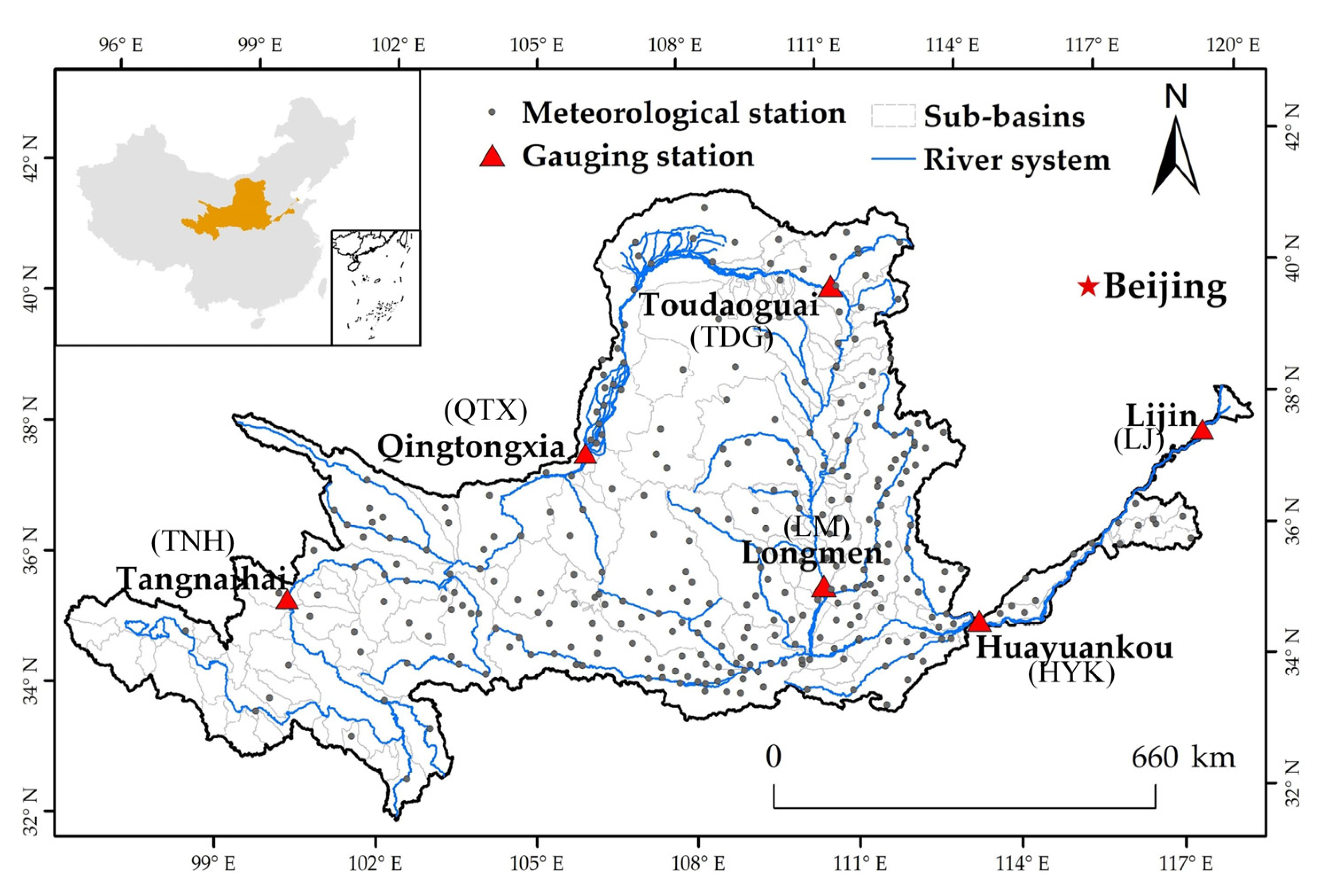
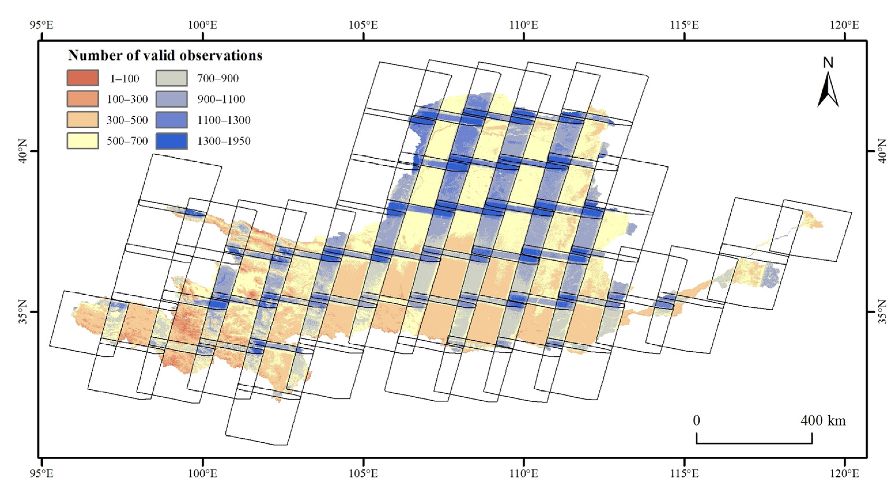
2.1. Study Area and Data Processing

The Yellow River is the second-longest river in China, with a total length of 5464 km. The YRB is mostly located in the semi-arid to semi-humid regions, where the mean annual precipitation ranges from 300 to 700 mm, and the average multi-year temperatures range from −4 to 14 °C. The multi-year average runoff volume and sediment discharge in the main river channel are 58 billion m³ and 1.6 billion tons [40], respectively. The top parts of the river are where the Yellow River flow originates, whereas the middle reaches are where the Yellow River sediment originates. In the upper and intermediate reaches, historic climate change and intensive human activities have resulted in substantial ecosystem deterioration. It has been reported that the underlying surface conditions have been dramatically changed, and that the ecological environment and the soil and water conservation capacity significantly improved after 2000, when extensive ecological restoration projects were implemented [41]. In addition, several large reservoirs have been gradually built on the main river channel by the national government for flow and sediment regulation and the optimal allocation of water resources in the YRB. In this study, the YRB was divided into six sub-regions based on the geographic locations of six key hydrological stations, including the Tangnaihai (TNH), Qingtongxia (QTX), Toudaoguai (TDG), Longmen (LM), Huayuankou (HYK), and Lijin (LJ) stations, located along the main river channel (Figure 1). The area above TNH is the source region of the YRB, and the area above TDG is the upper reaches of the YRB. The QTX-TDG sub-region is a typical windy desert area, and an irrigation area. The area between TDG and HYK is the middle reaches of the YRB, and the TDG-LM section is the main sediment formation area. The area between HKY and LJ is the upper reaches of the YRB. The upper reaches of the YRB are the main source area of the river runoff, and the middle reaches are the main source area of the sediments.

All of the available Landsat satellite images with a 30-m resolution (Landsat5 TM, Landsat7 ETM+ and Landsat8 OLI) covering the entire YRB from 1986 to 2019 were used in this study based on the Google Earth Engine platform (https://earthengine.google.com/, accessed on 16 March 2022), for which the Landsat ecosystem disturbance adaptive processing system (LEDAPS) [42] was employed to produce the surface reflectance of each Landsat pixel, and an F-mask algorithm [26,43] was then used to identify the contaminated pixels, such as clouds, cloud shadows and snow cover. The spatial distribution of the frequency of clear Landsat observations over the YRB from 1986 to 2019 is shown in the Figure 2, in which the effective number of observations in the northern region is larger than that in the southern region with more cloud coverage; the high values of observations occur in the area of overlapping satellite observations, and the low values are mainly distributed in the headwater region. Figure 3 depicts the interannual variation of the area ratio of the frequency with different levels (0–4, 5–10, 10–20, 20–40, 40–70, and 70–100) of clear Landsat observations over the YRB. It can be seen that as the Landsat satellite sensors were updated, the number of clear Landsat observations increased gradually. In addition, meteorological parameters including the daily precipitation (pre) and temperature (temp) during 1986–2019 of 295 stations located in the YRB were acquired from the China Meteorological Science Data Sharing Service (http://data.cma.cn/, accessed on 16 March 2022), and the raster data of the precipitation and temperature at the 1-km scale were produced using a spatial interpolation algorithm in the AUSPLINE software [44].

The global land surface satellite (GLASS) (http://www.glass.umd.edu/, accessed on 16 March 2022) [45] leaf area index (LAI) product with 8-day and 1-km resolution was selected to characterize the vegetation structure change during 1986–2019. Daily evapotranspiration (ET) and surface soil moisture (SM) data at 0.25° during 1986–2019 were derived from the Global Land Evaporation Amsterdam Model (GLEAM) (https://www.gleam.eu/, accessed on 16 March 2022 ) [46] v3.5a product. Finally, the daily meteorological parameters, 8-day LAI, daily ET and SM were temporally upscaled into annual total Pre and ET, and the annual average temp, LAI and SM.

2.2. Surface Water Body Mapping Algorithm

The water and vegetation index and the threshold-based method proposed by Zou et al. [23] were used in this study. The algorithms for the water and vegetation indices and threshold rules are as follows:

$$\mathrm{NDVI}=\frac{{\rho }_{NIR}-{\rho }_{red}}{{\rho }_{NIR}+{\rho }_{red}},$$

(1)

$$\mathrm{MNDWI}=\frac{{\rho }_{green}-{\rho }_{SWIR1}}{{\rho }_{green}-{\rho }_{SWIR1}},$$

(2)

$$\mathrm{EVI}=2.5\times \frac{{\rho }_{NIR}-{\rho }_{red}}{{\rho }_{NIR}+6\times {\rho }_{red}-7.5\times {\rho }_{biue}+1},$$

(3)

$$\mathrm{EVI}<0.1 \mathrm{and}\left(\mathrm{mNDWI}>\mathrm{NDVI} \mathrm{or} \mathrm{mNDWI}>\mathrm{EVI}\right)$$

(4)

where ${\rho }_{red}$, ${\rho }_{green}$, ${\rho }_{blue}$, ${\rho }_{NIR}$, and ${\rho }_{SWIR1}$ are the surface reflectance of the red, green, blue, near-infrared, and short-wave infrared wavelengths, respectively.

Because there are serious commission errors in the classified water bodies in shaded hills, the rule of terrain slopes of <8° was also employed in order to improve the identification accuracy of the water bodies in the hilly and mountainous areas [47]. Then, the Water Inundation Frequency (WIF) was calculated by dividing the number of identified water bodies by the number of clear Landsat observations in a year (Equation (4)). Water bodies with 25% ≤ WIF ≤ 75% were defined as seasonal water bodies, and water bodies with WIF > 75% were defined as permanent water bodies based on previous studies [48,49].

$$\mathrm{WIF}=\frac{W}{N}\times 100\%,$$

(5)

where N is the total number of valid observations in a year, and W is the total number of times the water body was detected.

Except for the SWA of the seasonal and permanent water bodies, the annual maximum SWA was calculated based on the water bodies with WIF ≥ 25%, and the annual average SWA was defined as the sum of all of the effective areas (900 m²) in one Landsat pixel multiplied by the WIF [23,24]. Therefore, the inter-annual time series of the four types of SWA (permanent, seasonal, annual maximum, and annual average water body areas) for the different sub-regions and different sub-basins was derived in order to analyze the spatial–temporal changes.

2.3. Accuracy Assessment

In order to assess the classification accuracy of the water bodies derived in this study, we selected 995 samples containing typical types of water bodies (rivers, lakes, reservoirs, and check dams) via artificial visual interpretation based on the high spatial resolution Google Earth images. Because the high-resolution Google Earth images were all acquired during 2019–2020, we only evaluated the accuracy of the water body classification in 2019 using the Google Earth Engine. In addition, we compared the accuracies of the water bodies identified using different WIF thresholds (5%, 10%, 15%, 25%, 35%, 50%, and 75%).

2.4. Linear Slope Calculation

In order to reveal the temporal variation characteristics of the SWA over time in the YRB, we used the slope of the linear regression model to characterize the interannual rate of change of the SWA during 1986–2019 in the YRB. The slope was calculated as follows:

$$\mathrm{Slope}=\frac{n\times {{\displaystyle \sum }}_i^{n}i\times X_i-{{\displaystyle \sum }}_{i=1}^{n}i{{\displaystyle \sum }}_{i=1}^n{X}_i}{n\times {{\displaystyle \sum }}_{i=1}^n{i}^2-{\left({{\displaystyle \sum }}_{i=1}^{n}i\right)}^2}$$

(6)

where X_i is the SWA in year i, and n is the total number of years. When the slope is >0, the SWA is increasing; and when the slope is <0, the SWA is decreasing.

Then, the slopes of the seasonal, permanent, annual maximum, and annual average SWAs in the entire YRB were analyzed, and the contributions of the SWAs in the different sub-regions and different sub-basins were compared.

2.5. Partial Correlation Analysis

Rainfall is the main source of surface water bodies, an increased temperature can increase the evaporation from surface water surfaces, vegetation is linked to evapotranspiration from surface water surfaces, and soil moisture influences temperature and rainfall. In order to explore the impacts of the natural water supply, atmospheric warming, vegetation greening, and SM on the SWA, we conducted a partial correlation analysis to examine the relationships between the SWA and the climatic parameters, vegetation status, and water storage status of the surface soil. Partial correlation analysis measures the strength and direction of a linear relationship between two variables while the effect of one or more other variables is controlled. In this way, the individual roles of the influencing factors in the SWA dynamics can be determined. The partial correlation coefficient was calculated as follows:

$$r_{i,j·l_1{l}_{2\dots \dots }{l}_n}=\frac{r_{i,j·l_1{l}_{2\dots \dots }{l}_{n-1}}-r_{i,l_n·l_1{l}_{2\dots \dots }{l}_{n-1}}·r_{j,l_n·l_1{l}_{2\dots \dots }{l}_{n-1}}}{\sqrt{\left(1-r_{i,l_n·l_1{l}_{2\dots \dots }{l}_{n-1}}^2\right)·\left(1-r_{j,l_n·l_1{l}_{2\dots \dots }{l}_{n-1}}^2\right)}}$$

(7)

where $r_{i,j·l_1{l}_{2\dots \dots }{l}_n}$ is the nth (n = k − 2) order partial correlation coefficient between i and j when l₁, l₂ … l_n are controlled, and k is the total number of variables. $r_{i,l_n·l_1{l}_{2\dots \dots }{l}_{n-1}}^2$ and $r_{j,l_n·l_1{l}_{2\dots \dots }{l}_{n-1}}^2$ are the (n − 1)th order partial correlation coefficient. When $r_{i,j·l_1{l}_{2\dots \dots }{l}_n}$> 0, the relationship between i and j is positive; otherwise, it is negative.

We also examined the significance of this correlation by performing hypothesis testing.

$$t=\frac{\sqrt{m-\mathrm{k}-2}·r_{i,j·l_1{l}_{2\dots \dots }{l}_n}}{\sqrt{1-r_{i,j·l_1{l}_{2\dots \dots }{l}_{n-1}}^2}}$$

(8)

where t is the t-test value, m is the sample size (here m = 34), and k is the degree of freedom. When t < 0.05, the partial correlation is statistically significant (at the 95% statistical significance level).

3. Results

3.1. Surface Water Body Classification Results and Accuracy Validation

The WIF in the YRB was calculated for each year from 1986 to 2019, and the WIFs of six typical surface water bodies in the YRB are presented in Figure 4. The SWA of Hongjiannao Lake gradually decreased, whereas the SWA of Longyangxia Reservoir increased. The SWA of the Xiaolangdi Reservoir increased abruptly due to reservoir storage after it began operating. The SWA of Wuliangsuhai Lake fluctuated sharply between years due to rainfall and artificial water diversion. It can be seen that the SWA in the check dam increased gradually, which demonstrates that the check dam constructed in the 1980s not only intercepted large amounts of sediment but also served as a water storage facility for local irrigation. It can also be seen that the downstream river regime in Kaifeng changed dramatically, and the river regime became relatively stable after 2015. It can be reasonably concluded that the temporal variation in the WIF can effectively reflect the dynamics of the different surface water bodies in the different regions.

The classification accuracy of the surface water bodies derived using different WIF thresholds was validated based on selected samples of typical types of water bodies. The results show that the classification accuracies of the water bodies using WIF thresholds of 5%, 10%, 15%, 25%, 35%, 50%, and 75% were 97.33%, 97.23%, 97.17%, 97.12%, 97.00%, 96.86%, and 96.38%, respectively (Figure 5). The average value of the classification accuracy was as high as 97.01%, indicating that the surface water identification algorithm used in this study is very accurate and robust.

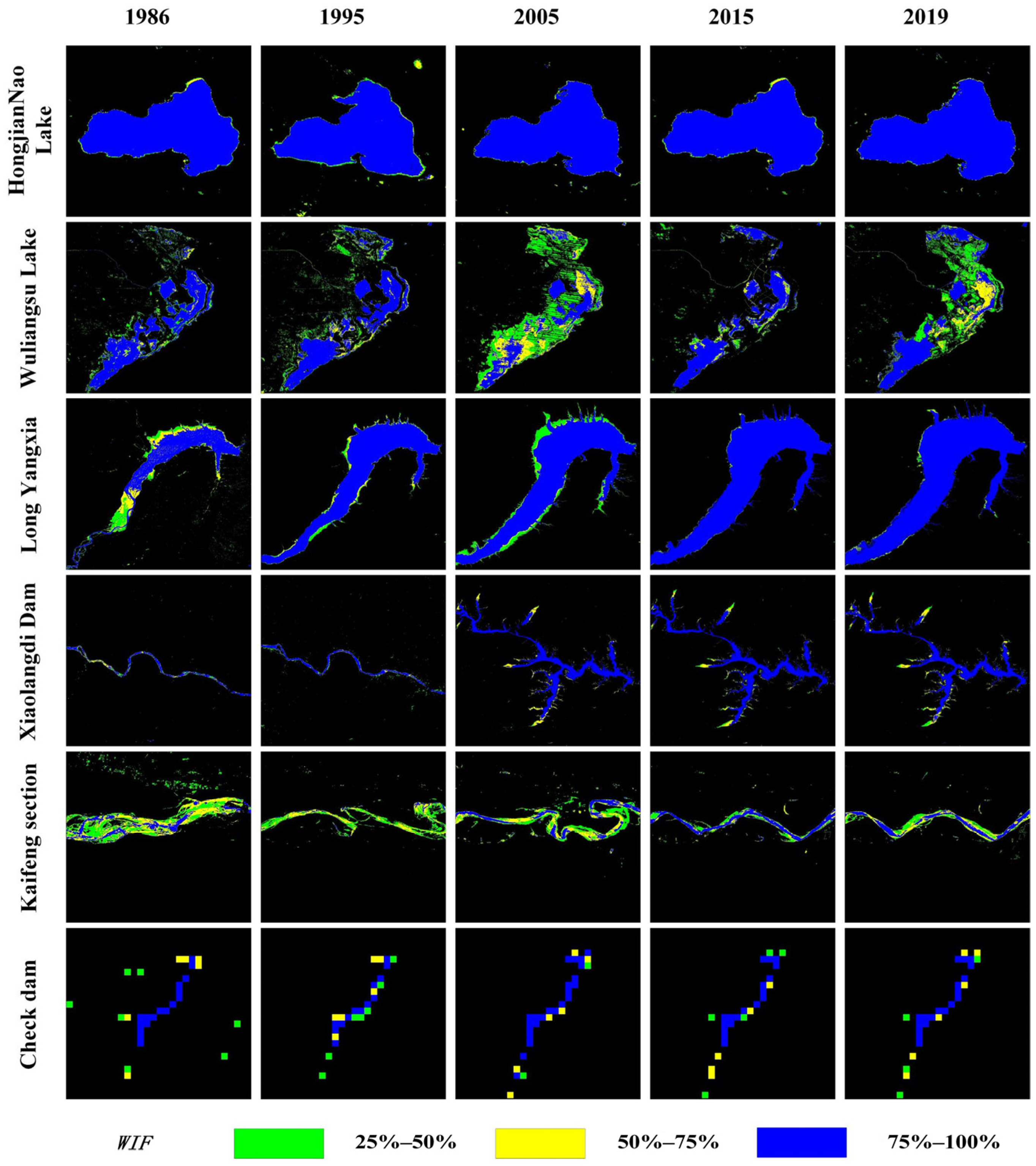
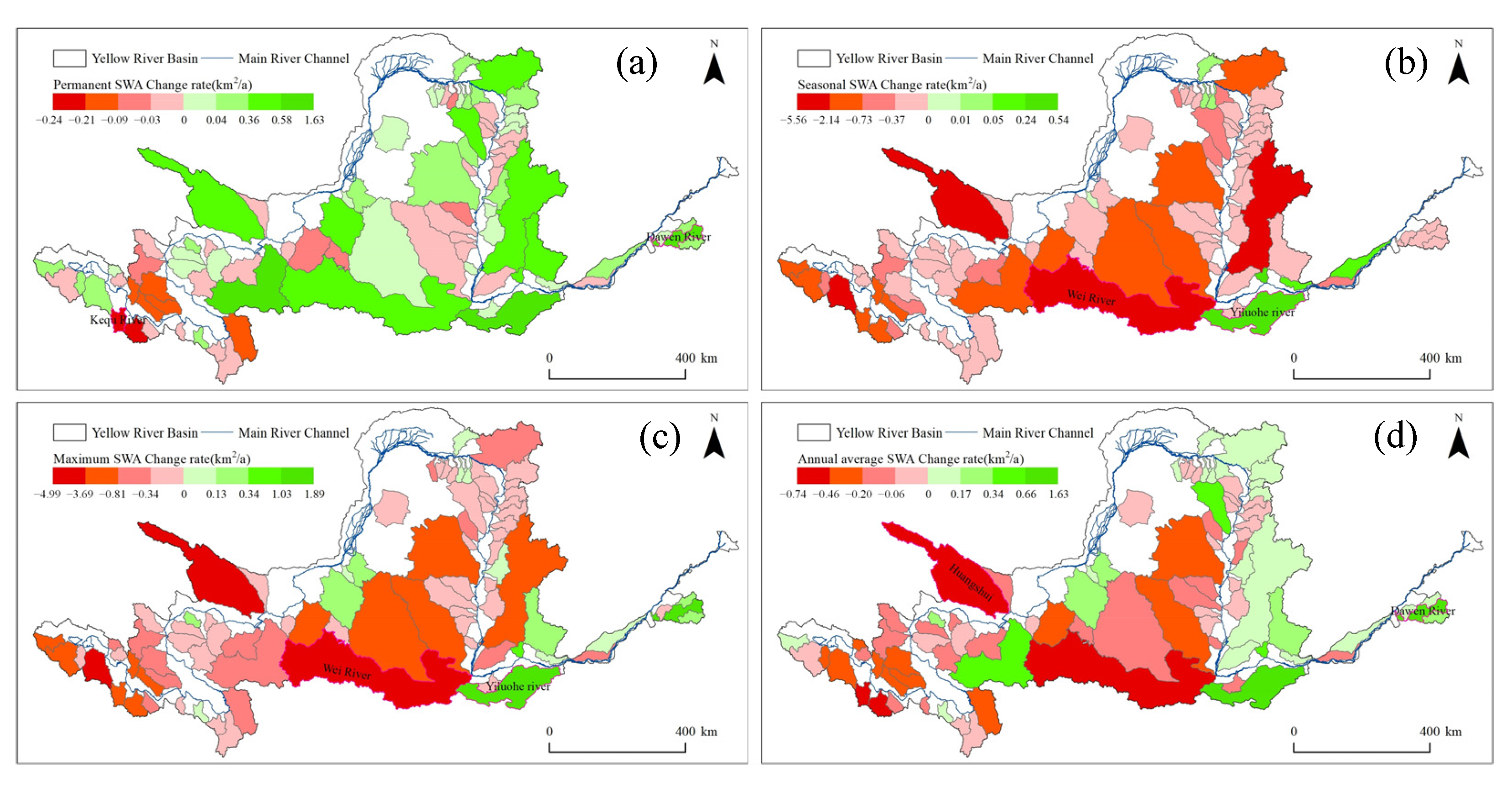
3.2. Spatial Distribution of the Surface Water Bodies in the YRB

The spatial distribution of permanent and seasonal water bodies derived from the multi-year average WIF during 1986–2019 is shown in Figure 6. It can be seen that the seasonal water bodies always existed in the transition areas between the permanent water bodies and the non-water bodies, and there were more seasonal water bodies near the river channel.

The different types of SWAs in all of the sub-regions of the YRB were calculated (Figure 7). For the entire YRB, the permanent water bodies covered an area of 4048.76 km², and the seasonal water bodies covered an area of 4661.69 km², accounting for 46.48% and 53.52% of the surface water bodies in the YRB, respectively. The maximum water body area was 8710.45 km², and the annual average water body area was 5853.17 km². The SWA in the source area of the upper reaches and the upstream area of the Yellow River (above Toudaoguai) contained 58.75% of the water bodies in the YRB, while the Huayuankou-Lijin segment contained 18.86%. The Toudaoguai–Longmen and Longmen–Huayuankou intervals contained 9.74% and 12.86% of the maximum water bodies in the YRB, respectively. These results indicate that the YRB was dominated by seasonal water bodies. However, it can be seen that the Tangnaihai section had far more permanent water bodies than seasonal water bodies. In the source region, the ratio of permanent to seasonal water bodies was 3.24, whereas the ratios in the Tangnaihai–Qingtongxia, Qingtongxia–Toudaoguai, Toudaoguai–Longmen, Longmen–Huayuankou, and Huayuankou–Lijin sections were 1.55, 0.27, 0.70, 0.33, and 0.55, respectively.

Figure 8 shows the statistical areas of the different types of water bodies in the selected 86 sub-basins in the YRB. The Wei River (101.18 km²) was the largest seasonal water body, and the Xianchuan River (0.07 km²) was the smallest. The Shushui River (58.96 km²) was the largest permanent water body, and the Mangla River was the smallest (0 km²). In terms of the major water bodies, the Wei River had the largest area (135.63 km²), and the Mangla River had the smallest area (0.08 km²). For the annual average water bodies, the Shushui River (80.94 km²) had the largest area, and the Mangla River (0.03 km²) had the smallest area.

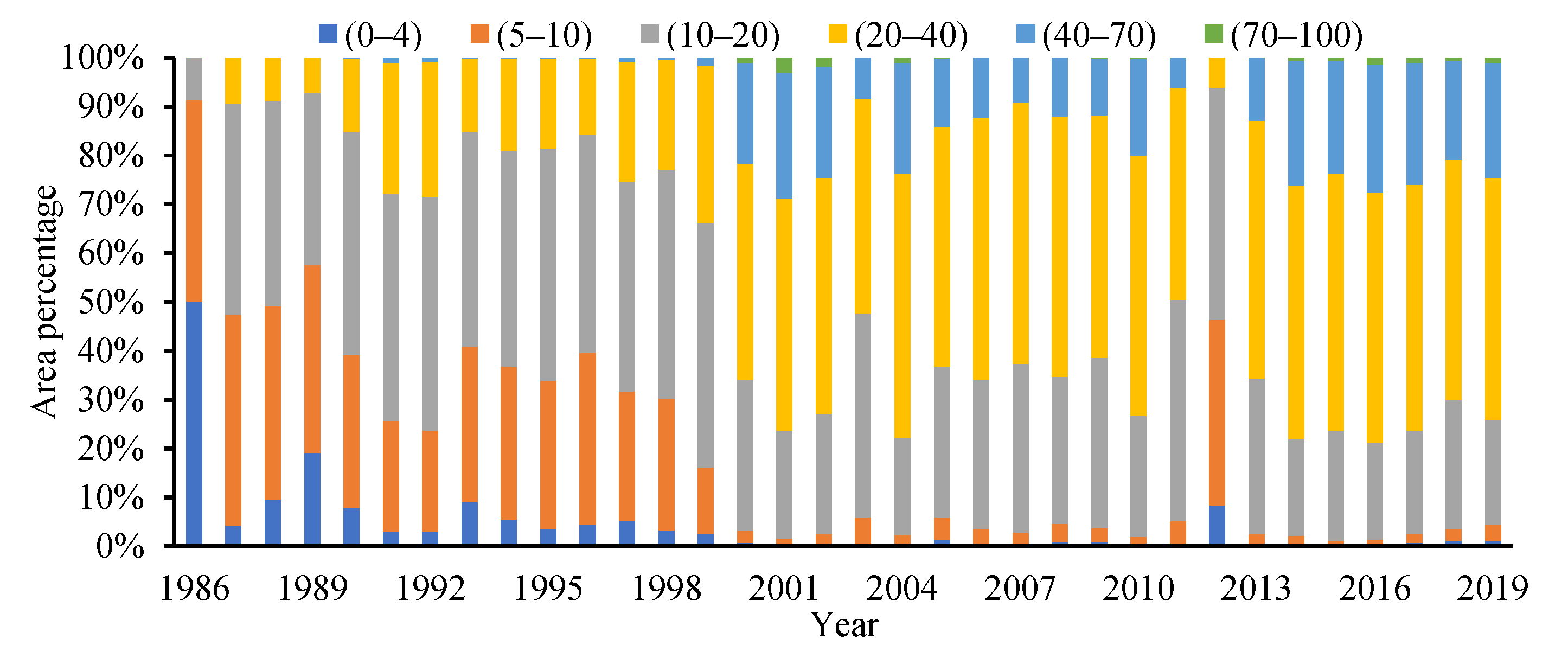
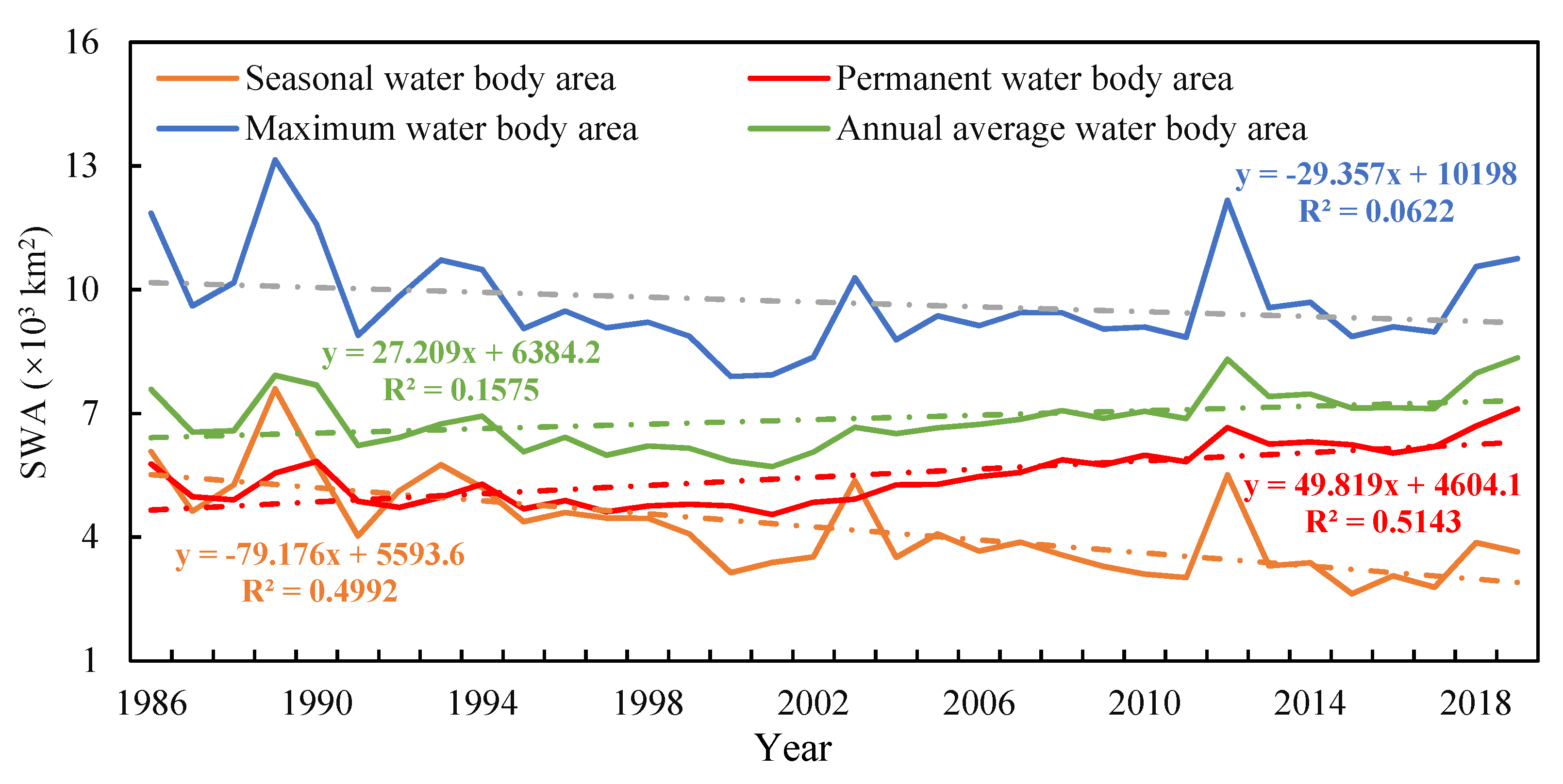
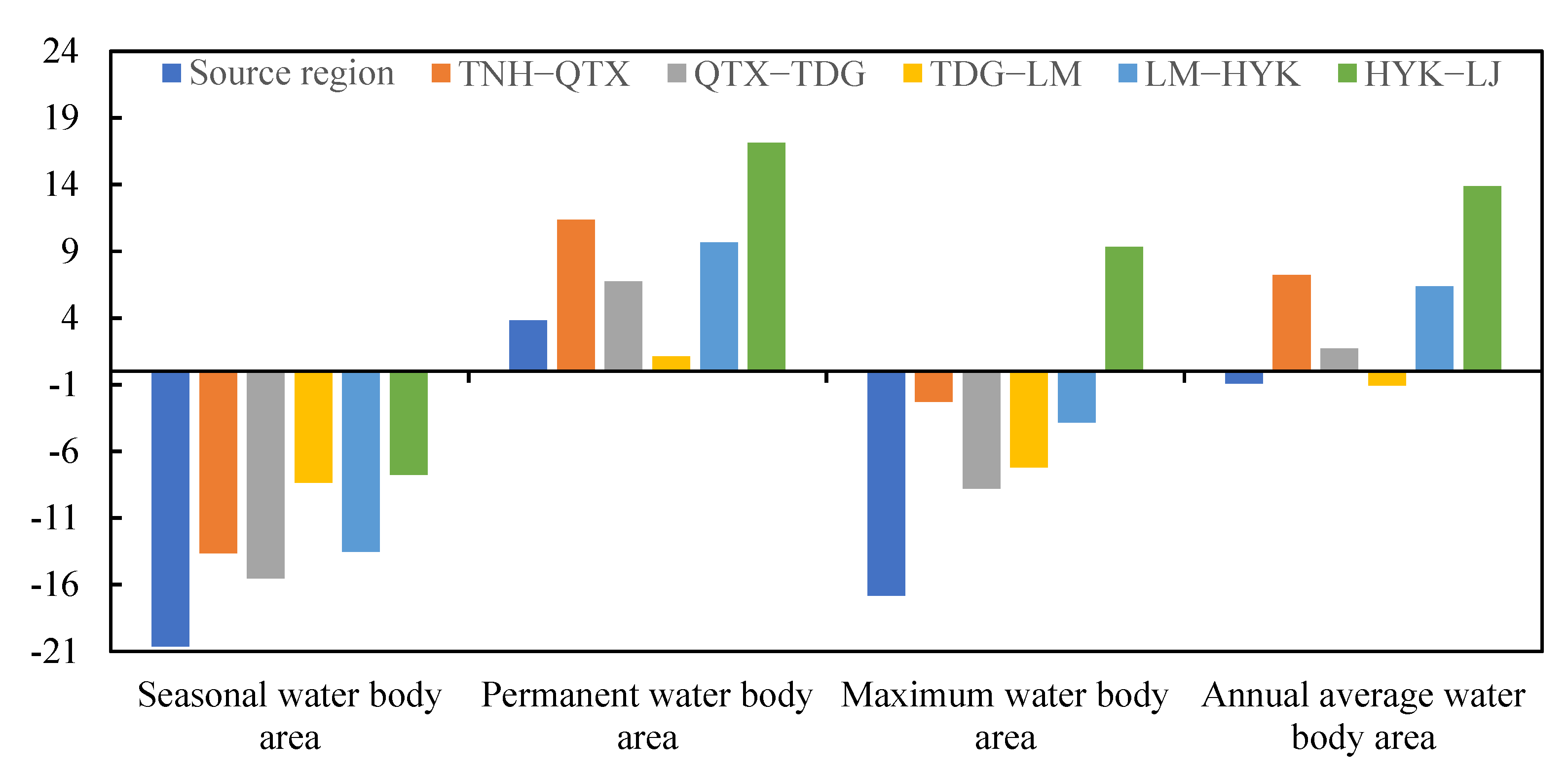
3.3. Changes in the SWA in the YRB from 1986 to 2019

Figure 9 shows the continuous dynamic changes in the different types of water bodies—including the seasonal, permanent, maximum, and annual average water bodies—in the entire YRB during 1986–2019. The maximum and seasonal water body areas exhibited typical decreasing trends from 1986 to 2019, but the permanent and annual water areas exhibited slightly increasing trends. The maximum water area varied from 7984.02 km² to 13,145.55 km², i.e., 35.75% higher and 18.48% lower than the average area of 9683.99 km², respectively. The permanent water area varied from 4547.8 km² to 7109.7 km², i.e., 16.95% lower and 29.84% higher than the average value (5475.95 km²), respectively. The seasonal water area varied from 2624.57 km² to 7595.80 km² during a single year, i.e., 37.63% lower and 80.51% higher than the average value (4208.04 km²), respectively. Because the average water area was based on the pixel level of the water bodies, it reflects the changes in the water bodies in one year the best. The annual water area varied from 5708.17 km² to 8344.84 km², i.e., 16.8% lower and 21.64% higher than the average value (6860.40 km²), respectively. As is shown in Figure 6, the statistics of the water bodies reveal decreasing trends in the maximum water body area (p < 0.01) and the seasonal water body area (p < 0.01) from 1986 to 2019. The permanent water area (p < 0.01) and the annual water body area (p < 0.01) exhibited increasing trends. The total SWA of the YRB initially decreased and then increased during the study period. According to the linear regression model, the annual water area in the YRB increased by 27.2 km² per year from 1986 to 2019.

Figure 10 depicts the changes in the different types of water bodies in six sub-regions in the YRB. The seasonal water bodies exhibited decreasing trends in all six sub-regions. The source area had the largest rate of change of −20.66 km²/a, accounting for 25.99%. The permanent water bodies exhibited increasing trends in all six sub-regions. The Huayuankou–Lijin section had the largest rate of change of 17.1 km²/a, accounting for 34.34%. Among the remaining subdivisions, in section Huayuankou–Lijin, the largest water body exhibited an increasing trend (9.33 km²/a); the source area had the largest negative trend (16.85 km²/a), accounting for 34.87%. Except for in the source region and the Toudaoguai–Longmen section, which exhibited minor decreasing trends of roughly −1 km²/a, the Huayuankou–Lijin section continued to have the strongest increasing trend in terms of the annual mean water bodies (13.85 km²/a), accounting for 44.48% in the entire YRB.

Figure 11 depicts the rates of change of the various types of water bodies in the 86 sub-basins of the YRB from 1986 to 2019. The Dawen River basin had the highest permanent SWA growth rate (1.63 km²/a), whereas the Kequ River basin had the highest permanent SWA reduction rate (−0.24 km²/a). The Yiluohe River (0.54 km²/a) had the highest seasonal SWA growth rate, and the Wei River (−5.56 km²/a) had the highest seasonal SWA reduction rate. The Yiluohe River (1.89 km²/a) had the highest maximum SWA growth rate, and the Wei River (−4.99 km²/a) had the highest maximum SWA reduction rate. The Dawen River (1.63 km²/a) had the highest annual average SWA growth rate, and the Huangshui (−0.74 km²/a) had the highest reduction rate.

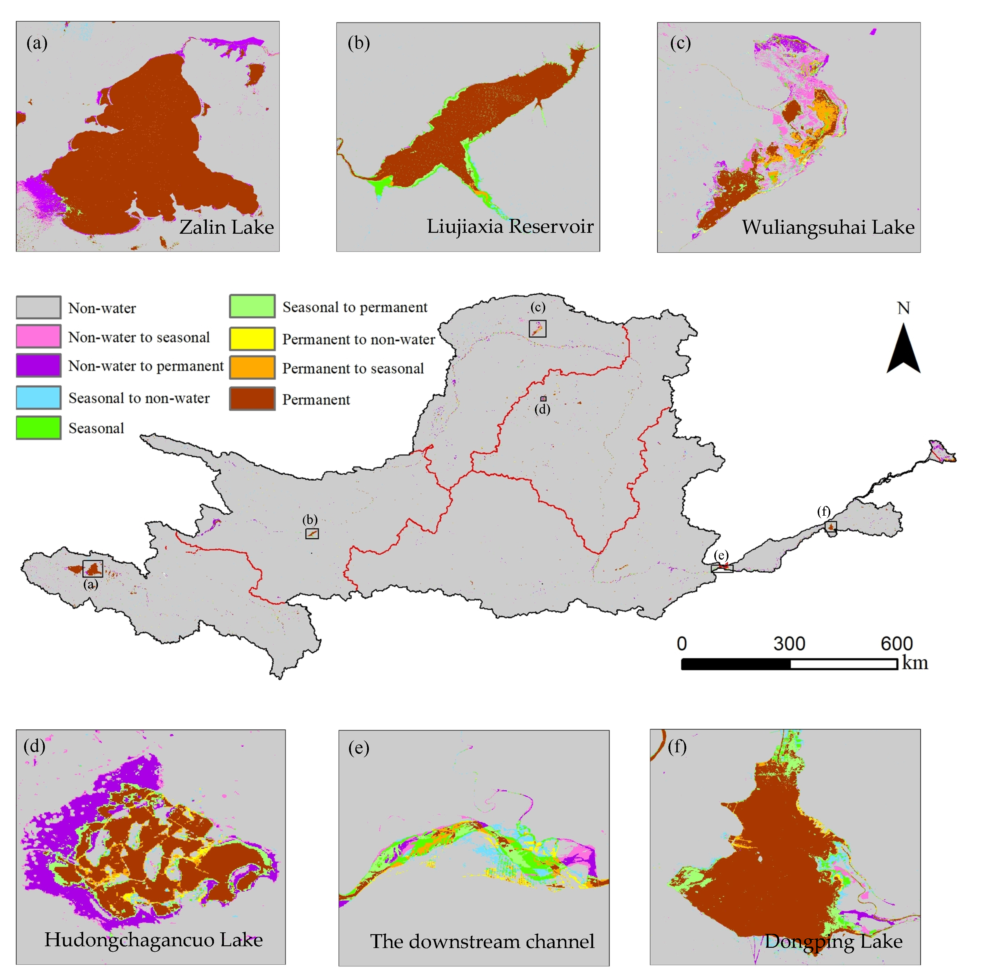
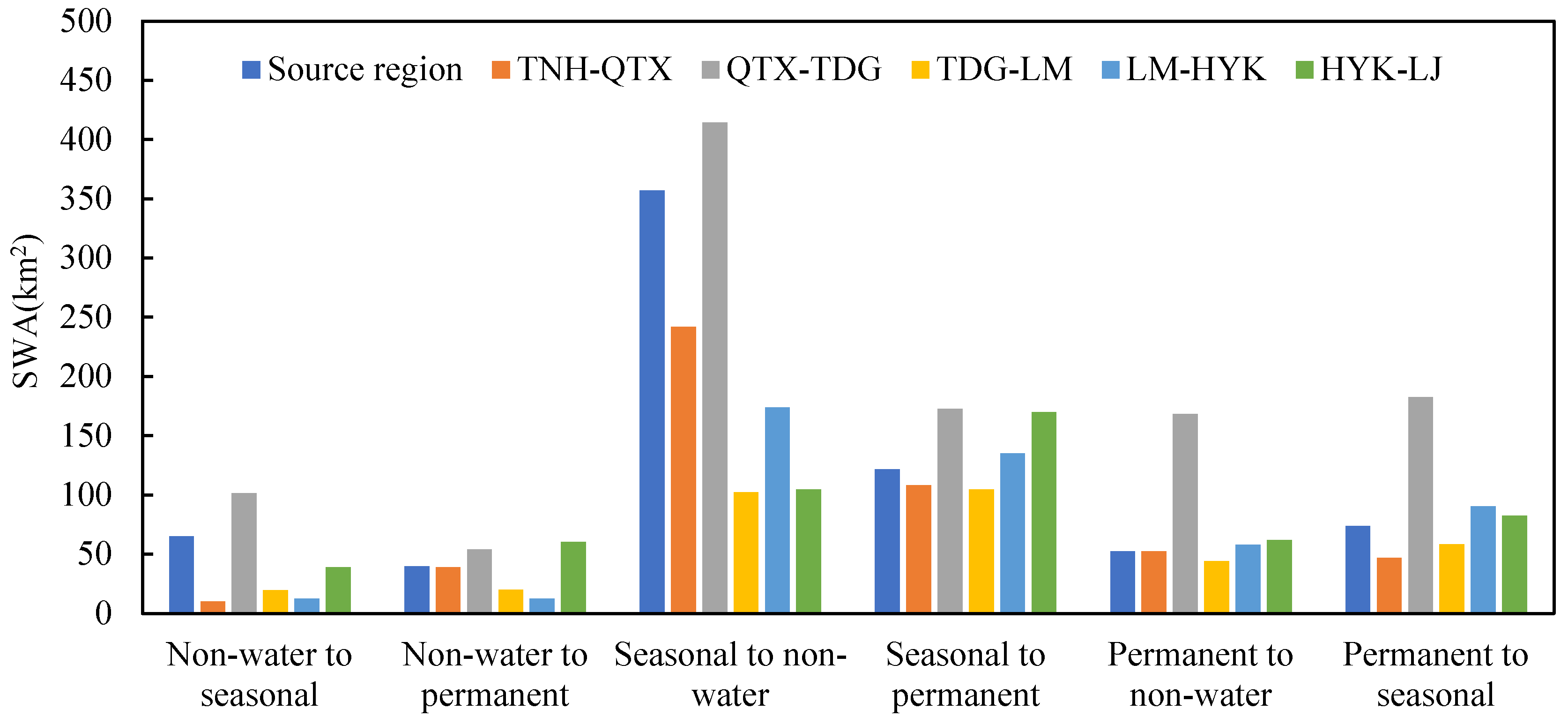
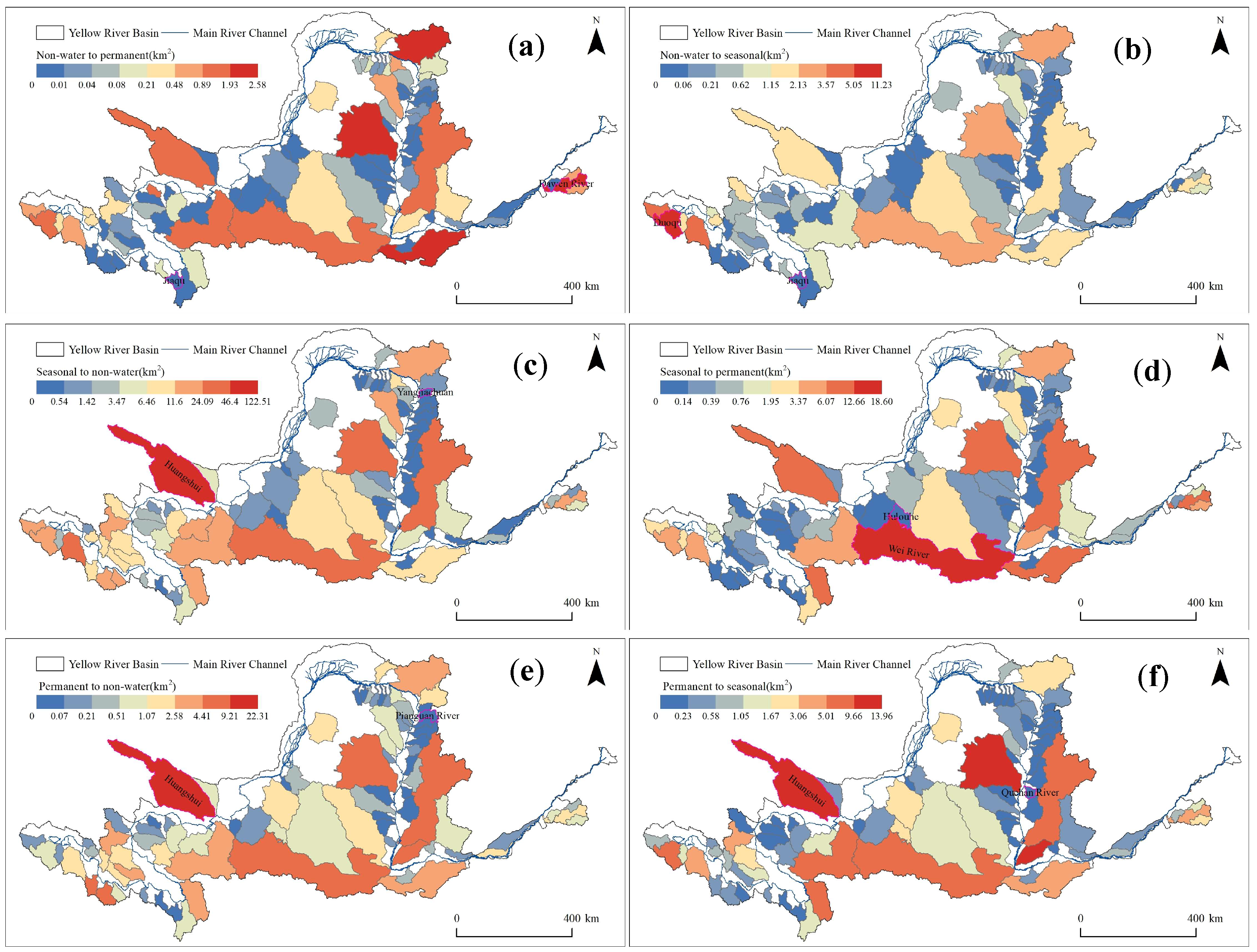
3.4. Conversions of Different Types of Surface Water Bodies

The types of conversions between different water bodies from 1986 to 2019 were divided into non-water to seasonal, non-water to permanent, seasonal to non-water, seasonal to permanent, permanent to non-water, and permanent to seasonal conversions. The spatial pattern of the different conversion types is shown in Figure 12 and Figure 13. The most common conversion in the source region was from seasonal to non-water bodies, with a conversion area of 357.05 km², while the least common conversion was from non-water bodies to permanent water bodies, with a conversion area of 39.7 km². With a conversion area of 241.87 km², the conversions from seasonal to non-water bodies were the most prevalent in the Tangnaihai–Qingtongxia section. Conversely, the conversions from non-water bodies to seasonal water bodies were the least common, with a conversion area of 10.03 km². The transition from non-water bodies to permanent water bodies was the least common in the Qingtongxia–Toudaoguai section, whereas the transition from seasonal to non-water bodies was the most common, with a conversion area of 414.35 km². In the Toudaoguai–Longmen section, the most common transformation was from seasonal to permanent water bodies, with a conversion area of 104.5 km², while the least common transformation was from non-water bodies to seasonal water bodies, with a conversion area of 19.62 km². Hua’s long scenario is comparable to that in the Qingtongxia–Toudaoguai section, in which the least common change was from non-water bodies to permanent water bodies, with a conversion area of 12.2 km², while the most frequent transformation was from seasonal to non-water bodies, with a conversion area of 173.75 km².

Figure 14 further shows the SWAs of the different water body conversion types in each sub-basin. It can be seen that the conversion of water bodies in the YRB exhibited strong spatial heterogeneity. The largest conversion of non-water bodies to permanent water bodies occurred in the Dawen River (2.58 km²), and the smallest occurred in Jiaqu (0 km²). The largest conversion of non-water bodies to seasonal water bodies occurred in the Duoqu (11.23 km²) and the smallest occurred in Jiaqu (0 km²). The largest conversion of seasonal water bodies to non-water bodies occurred in Huangshui (122.51 km²) and the smallest occurred in Yangjiachuan (0 km²). The largest conversion of seasonal water bodies to permanent water bodies occurred in Weihe (18.60 km²) and the smallest occurred in Hulouhe (0 km²). The largest conversion of permanent water bodies to non-water bodies occurred in Huangshui (22.31 km²) and the smallest occurred in the Pianguan River (0 km²). The largest conversion of permanent water bodies to seasonal water bodies occurred in Huangshui (13.96 km²) and the smallest occurred in the Quchan River (0 km²).

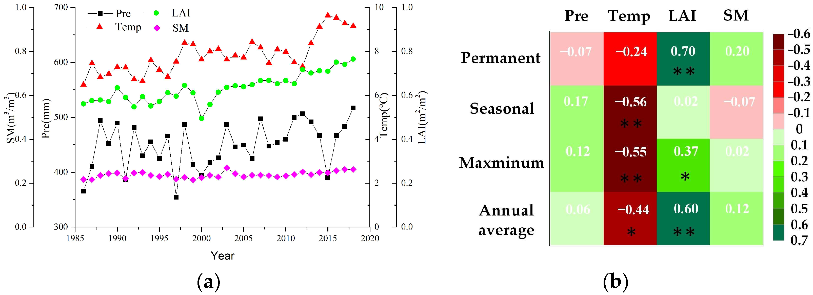
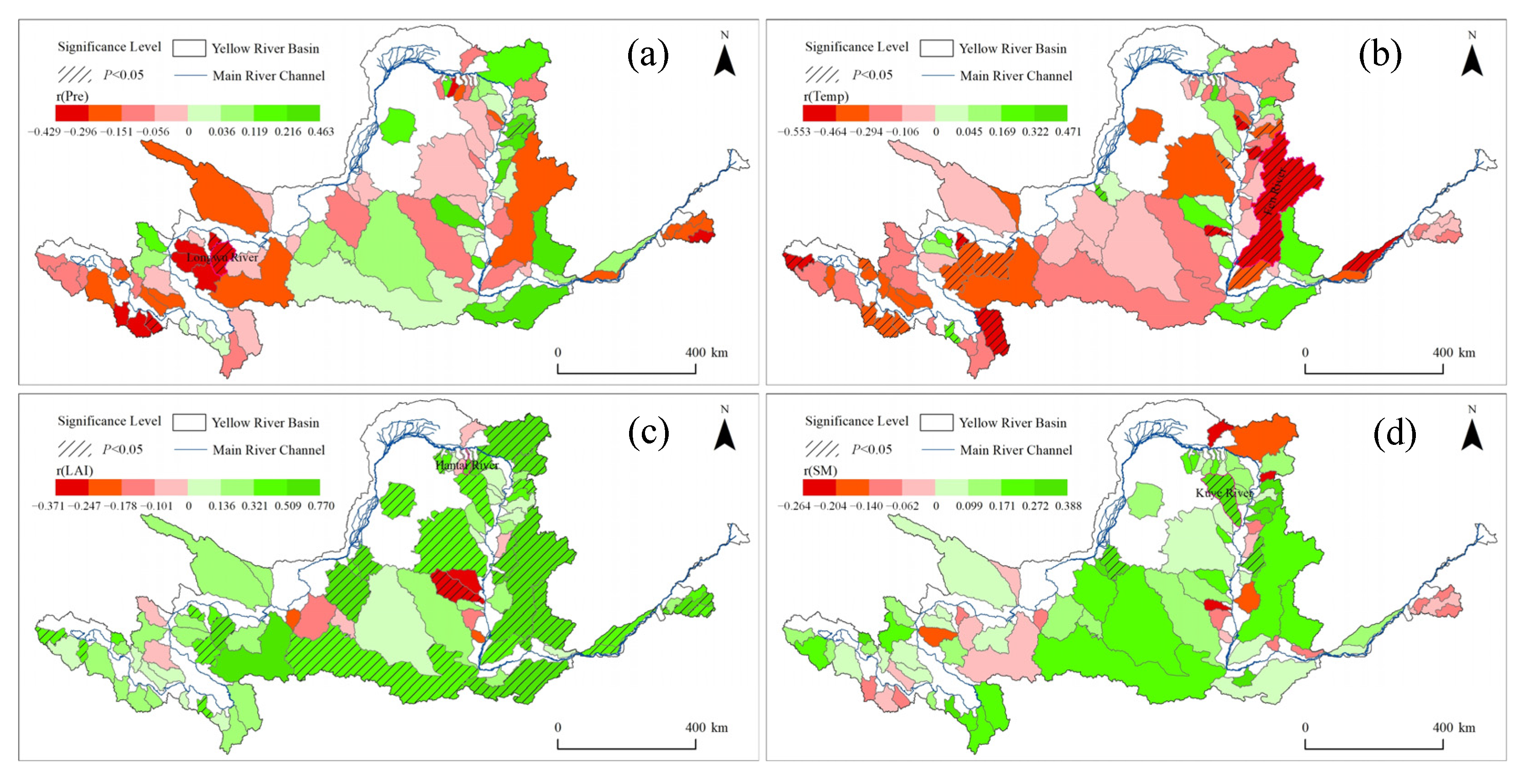
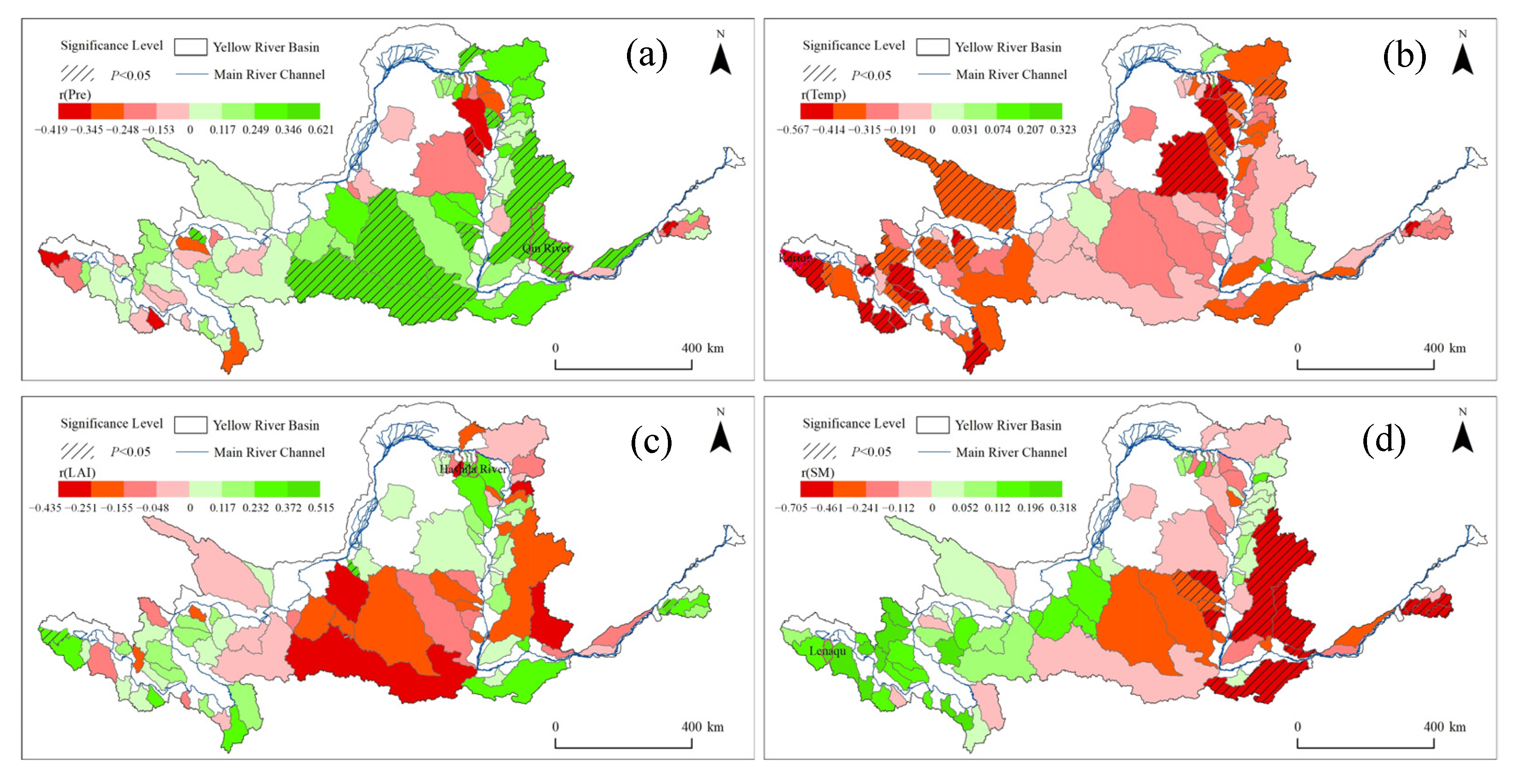
3.5. Relationship between SWA and Environmental Factors

In order to explore the impacts of the water supply, atmospheric warming, vegetation greening, and surface SM on the SWA, we conducted partial correlation analysis to derive the correlations between the SWA and the Pre, Temp, LAI, and SM. During 1986–2019, the Pre, LAI, Temp, and SM in the entire YRB all increased, with the rate of change of Pre was 1.69 km²/a, and the rates of change of LAI, Temp, and SM were not as large (Figure 15a). The partial correlation coefficients between the different types of water bodies and the Pre, Temp, LAI, and SM are shown in Figure 15b. The different types of water bodies were negatively correlated with temperature, while the LAI was positively correlated with the different types of water bodies. The creation of permanent water bodies was aided by an increase in the surface SM, which led to a small decrease in the seasonal water bodies. None of the correlations between Pre and the different types of water bodies were significant.

Divergent correlations between the SWA and the Pre, Temp, LAI, and SM were observed in the 86 sub-basins (Figure 16 and Figure 17). In terms of the permanent water bodies, in 62.8% of the sub-basins, which were primarily located in the source area, the correlation between Pre and SWA was negative, and the Longwu River had the highest negative correlation coefficient. The increase in temperature reduced the SWA in 76.7% of the watersheds, mostly in the source area and the upper and middle reaches, and the Fen River had the largest negative correlation coefficient. The correlation between the LAI and SWA was positive in 86% of the watersheds, spanning the entire YRB, and the Hantai River had the highest positive correlation coefficient. The correlation between the SM and SWA was positive in 70.9% of the watersheds, mostly in the middle reaches, and the Kuye River had the highest positive correlation coefficient. The correlations between Pre and SWA were essentially not significant, whereas the associations between the SWA and the temperature, LAI, and SM were all significant to varying degrees.

In terms of the seasonal water bodies, the correlation between Pre and SWA was positive in 67.4% of the sub-basins, mostly in the middle reaches, and the Qin River had the highest positive correlation coefficient. The SWA decreased with the increasing temperature in 94.2% of the watersheds in the YRB, and the negative correlation coefficient of Kariqu was the highest. In 55.8% of the watersheds, LAI was positively correlated with SWA, primarily in the middle reaches, and the Hashila River had the largest positive effect on the SWA. In 55.8% of the watersheds, SM was positively correlated with the SWA, primarily in the source and upstream areas, and Lenaqu had the highest positive correlation coefficient. LAI was insignificantly correlated with the SWA, but the correlations between the SWA and the Pre, Temp, and SM were all significant at different levels.

4. Discussion

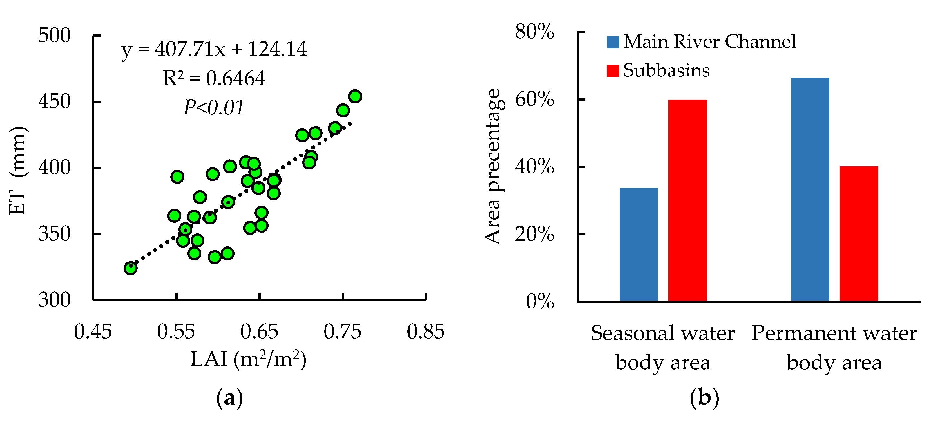
4.1. Potential Influence Mechanism of the Environmental Factors on the SWA

Natural rainfall is the main water resource of the surface water bodies in the YRB; however, insignificant correlations between Pre and the different types of water bodies were observed (Figure 15), which indicate that Pre was not the dominant factor influencing the change in the SWA in the YRB during 1986–2019. An increase in temperature can increase the potential evaporation and the atmospheric vapor pressure deficit, accelerating the actual evaporation of surface water bodies [23]; Xia et al. came to the same conclusion in their study of the Huai River [26].

According to studies, a considerable increase or decrease in plant cover can alter surface water patterns [50]. An increase in the LAI can lower the land surface albedo, increase the solar radiation absorbed by the vegetation canopy, and increase the transpiration and interception evaporation from the vegetation [51] (Figure 18a). An increase in the latent heat can lead to a decrease in the land surface temperature and an increase in the air humidity, resulting in a decrease in the evaporation from surface water bodies [52]. Therefore, an increase in the vegetation LAI contributes to an increase in SWA [53,54], and Zeng et al. found the same pattern in studies in the Northeast China and Loess Plateau regions [55]. In addition, vegetation improves the surface runoff impedance and greatly enhances the trapped ET and soil water storage [56], which may alter the development of seasonal water bodies. Thus, seasonal water bodies are not strongly correlated with the LAI.

Soil moisture is an important variable in the water and energy cycle because it impacts how rainfall is divided into runoff, surface storage, and infiltration components, and how entering solar and long-wave radiation is divided into outgoing long-wave radiation, latent heat, and so on. Soil moisture is an important variable in the water and energy cycle. The surface temperature, on the other hand, is a key component in establishing the land surface’s heat and moisture balance. The surface temperature determines the incoming long-wave, sensible heat, and surface heat flow. Generally, the surface temperature shows an increase that corresponds to a decrease in the soil moisture [57]. However, the greater the surface SM is, the more easily the water storage soil layer becomes saturated, the longer the surface water body may persist after formation, and the more likely it is that a permanent water body will be established. As is illustrated in Figure 15 and Figure 16, the correlation between the SM and the SWA was positive for the permanent water bodies and negative for the seasonal water bodies.

Due to the definition of permanent and seasonal water bodies, a rise in permanent water bodies equals a loss in seasonal water bodies, with opposite trends in their changes and thus major variations in the impact of influencing variables on both. It should be noted that compared with the seasonal water bodies, the SWA of the permanent water bodies was less strongly correlated with the Pre and Temp, and was even negatively correlated with Pre (Figure 15 and Figure 16). This is mainly because most of the permanent water bodies are distributed in the main channel area (Figure 18b), and the storage and regulation effects of the large reservoirs located on the main channel have significantly influenced the SWA change in the channel area.

In contrast, the seasonal water bodies were generally located in the sub-basins where the effect of small-size reservoirs on SWA was less than that from large reservoirs located in the main channel; thus, the SWA change of the seasonal water bodies was more dependent on the natural precipitation and hydrological processes. However, the massive expansion of vegetation and water conservation engineering measures have significantly altered the precipitation redistribution through canopy interception, litter, and soil absorption [58,59], resulting in an insignificant correlation between the precipitation and surface water area [60].

4.2. Uncertainties

Despite the F-mask method having removed some clouds and cloud shadows from the remote sensing imagery, undetected thin clouds or mountain shadow areas still had an impact on the water body extraction in this investigation. Although the adopted hybrid index rule set for the water extraction had a high degree of accuracy, there were still some recognition mistakes based on comparisons with the Google Earth high-resolution photographs. The WIF thresholds used to distinguish between permanent and seasonal water bodies in this study were based on the findings of a vast number of previous studies, but these thresholds may vary with the location. In this study, the correlations between the SWA and various influencing factors were calculated using the partial correlation coefficient method, which only statistically analyzed the degree of correlation between the two changes, and did not quantitatively calculate the effects of the various influencing factors on the SWA. However, this study has taken into account the effects of the interactions between several contributing factors, which could reduce some uncertainties of the influence analysis. It should be also noted that due to the lack of groundwater observations, the effect of the groundwater supply on the SWA was neglected in this study.

5. Conclusions

In this study, we analyzed the spatial–temporal variability of the SWAs of four types of water bodies (permanent, seasonal, maximum, and average extents) and their relationships with precipitation (Pre), temperature (Temp), LAI, and surface SM using all of the available Landsat images acquired from 1986 to 2019 and a water and vegetation index-based method. The results demonstrate that the accuracy of the water body identification method used in this study was 97%, according to an accuracy verification based on high-resolution Google Earth images.

The YRB’s permanent SWA increased at a rate of 49.82 km²/y, with the largest proportion—34.34%—occurring in the downstream area, while the seasonal SWA decreased at a rate of 79.18 km²/y, with the largest proportion—25.99%—occurring in the source area. In 50 of the 86 sub-basins, the SWA of the permanent water bodies increased, and these sub-basins were mainly located in the middle and lower reaches. The SWA of the seasonal water bodies increased in five of the sub-basins, accounting for just 5.8% of the total, indicating that the changes in the SWA in the sub-basin areas were the primary driver of the decrease in the SWA of the seasonal water bodies. The conversions from seasonal water bodies to non-water and from seasonal to permanent water bodies were the dominant trends from 1986 to 2019 in the YRB.

For the permanent water bodies, the SWA was less strongly correlated with Pre and Temp, and it was negatively correlated with Pre (Figure 15 and Figure 16) because most of the permanent water bodies were distributed in the main channel area (Figure 18a), and the storage and regulation effects of the large terrace reservoirs located on the main channel significantly influenced the changes in the SWA in the channel area.

The seasonal water bodies were primarily located in the sub-basins, and the surface water was mostly controlled by natural hydrological processes. Thus, the SWA was more dependent on the climatic factors. An increase in the surface SM can lead to the establishment of permanent water bodies, as well as a reduction in seasonal water bodies. By modifying the local climatic conditions, a considerable increase in the ET due to increased vegetation may decrease the evaporation of the surface water, partially compensating for the faster evaporation of the water surface caused by the increased air temperature.

References

1. Amprako, J.L. The United Nations World Water Development Report 2015: Water for a Sustainable World. Future Food J. Food Agric. Soc. 2016, 4, 64–65. [Google Scholar]
2. Costanza, R.; d′Arge, R.; De Groot, R.; Farber, S.; Grasso, M.; Hannon, B.; Limburg, K.; Naeem, S.; O′Neill, R.V.; Paruelo, J.; et al. The value of the world′s ecosystem services and natural capital. Nature 1997, 387, 253. [Google Scholar] [CrossRef]
3. Wood, E.F.; Roundy, J.K.; Troy, T.J.; van Beek, L.P.H.; Bierkens, M.F.P.; Blyth, E.; de Roo, A.; Döll, P.; Ek, M.; Famiglietti, J.; et al. Hyperresolution global land surface modeling: Meeting a grand challenge for monitoring Earth′s terrestrial water. Water Resour. Res. 2011, 47, W05301. [Google Scholar] [CrossRef]
4. Shevyrnogov, A.P.; Kartushinsky, A.V.; Vysotskaya, G.S. Application of Satellite Data for Investigation of Dynamic Processes in Inland Water Bodies: Lake Shira (Khakasia, Siberia), A Case Study. Aquat. Ecol. 2002, 36, 153–164. [Google Scholar] [CrossRef]
5. Rabus, B.; Eineder, M.; Roth, A.; Bamler, R. The Shuttle Radar Topography Mission—A New Class of Digital Elevation Models Acquired by Spaceborne Radar. ISPRS J. Photogramm. Remote Sens. 2003, 57, 241–262. [Google Scholar] [CrossRef]
6. Hall, J.W.; Grey, D.; Garrick, D.; Fung, F.; Brown, C.; Dadson, S.J.; Sadoff, C.W. Coping with the curse of freshwater variability. Science 2014, 346, 429–430. [Google Scholar] [CrossRef]
7. Tulbure, M.G.; Broich, M.; Stehman, S.V.; Kommareddy, A. Surface water extent dynamics from three decades of seasonally continuous Landsat time series at subcontinental scale in a semi-arid region. Remote Sens. Environ. 2016, 178, 142–157. [Google Scholar] [CrossRef]
8. Huang, C.; Chen, Y.; Zhang, S.; Wu, J. Detecting, extracting, and monitoring surface water from space using optical sensors: A review. Rev. Geophys. 2018, 56, 333–360. [Google Scholar] [CrossRef]
9. Cole, J.J.; Prairie, Y.T.; Caraco, N.F.; McDowell, W.H.; Tranvik, L.J.; Striegl, R.G.; Duarte, C.M.; Kortelainen, P.; Downing, J.A.; Middelburg, J.J. Plumbing the Global Carbon Cycle: Integrating Inland Waters into the Terrestrial Carbon Budget. Ecosystems 2007, 10, 172–185. [Google Scholar] [CrossRef] [Green Version]
10. Carroll, M.L.; Townshend, J.R.G.; DiMiceli, C.M.; Loboda, T.; Sohlberg, R.A. Shrinking Lakes of the Arctic: Spatial Relationships and Trajectory of Change. Geophys. Res. Lett. 2011, 38, L20406. [Google Scholar] [CrossRef] [Green Version]
11. Craglia, M.; de Bie, K.; Jackson, D.; Pesaresi, M.; Remetey-Fülöpp, G.; Wang, C.; Annoni, A.; Bian, L.; Campbell, F.; Ehlers, M. Digital Earth 2020: Towards the Vision for the next Decade. Int. J. Digit. Earth 2012, 5, 4–21. [Google Scholar] [CrossRef]
12. Jianbo, L.; Changda, D. The application of TM image in reservoir situation monitoring. Natl. Remote Sens. Bull. 1996, 1, 54–58. [Google Scholar]
13. Bi, H.Y.; Wang, S.Y.; Zeng, J.Y.; Zhao, Y.; Wang, H.; Yin, H. Comparison and analysis of several common water extraction methods based on TM image. Remote Sens. Inf. 2012, 27, 77–82. [Google Scholar]
14. Jiaju, L.; Shihong, L. Improvement of the techniques for distinguishing water bodies from TM data. J. Remote Sens. 1992, 1, 17–23. [Google Scholar]
15. McFeeters, S.K. The use of the Normalized Difference Water Index (NDWI) in the delineation of open water features. Int. J. Remote Sens. 1996, 17, 1425–1432. [Google Scholar] [CrossRef]
16. Xu, H. A study on information extraction of water body with the modified normalized difference water index (MNDWI). J. Remote Sens. 2005, 9, 589–595. [Google Scholar]
17. Xu, H. Modification of normalised difference water index (NDWI) to enhance open water features in remotelysensed imagery. Int. J. Remote Sens. 2006, 27, 3025–3033. [Google Scholar] [CrossRef]
18. Lei, J.I.; Zhang, L.I.; Wylie, B. Analysis of Dynamic Thresholds for the Normalized Difference Water Index. Photogramm. Eng. Remote Sens. 2009, 75, 1307–1317. [Google Scholar]
19. Verpoorter, C.; Kutser, T.; Tranvik, L. Automated Mapping of Water Bodies Using Landsat Multispectral Data. Limnol. Oceanogr. Methods 2015, 10, 1037–1050. [Google Scholar] [CrossRef]
20. Santoro, M.; Wegmueller, U.; Lamarche, C.; Bontemps, S.; Defoumy, P.; Arino, O. Strengths and weaknesses of multi-year Envisat ASAR backscatter measurements to map permanent open water bodies at global scale. Remote Sens. Environ. 2015, 171, 185–201. [Google Scholar] [CrossRef]
21. Gómez, C.; White, J.C.; Wulder, M.A. Optical remotely sensed time series data for land cover classification: A review. ISPRS J. Photogramm. Remote Sens. 2016, 116, 55–72. [Google Scholar] [CrossRef] [Green Version]
22. Khatami, R.; Mountrakis, G.; Stehman, S.V. A meta-analysis of remote sensing research on supervised pixel-based land-cover image classification processes: General guidelines for practitioners and future research. Remote Sens. Environ. 2016, 177, 89–100. [Google Scholar] [CrossRef] [Green Version]
23. Zou, Z.H.; Dong, J.W.; Menarguez, M.A.; Xiao, X.M.; QIN, Y.W.; Doughty, R.B.; Hooker, K.V.; Hambright, K.D. Continued decrease of open surface water body area in Oklahoma during 1984–2015. Sci. Total Environ. 2017, 595, 451–460. [Google Scholar] [CrossRef]
24. Zou, Z.H.; Xiao, X.M.; Dong, J.W.; Qin, Y.W.; Doughty, R.B.; Menarguez, M.A.; Zhang, G.L.; Wang, J. Divergent trends of open-surface water body area in the contiguous United States from 1984 to 2016. Proc. Natl. Acad. Sci. USA 2018, 115, 3810–3815. [Google Scholar] [CrossRef] [Green Version]
25. Liu, X.P.; Hu, G.H.; Chen, Y.M.; Li, X.; Xu, X.C.; Li, S.Y.; Pei, F.S.; Wang, S.J. High-resolution multi-temporal mapping of global urban land using Landsat images based on the Google Earth Engine Platform. Remote Sens. Environ. 2018, 209, 227–239. [Google Scholar] [CrossRef]
26. Xia, H.M.; Zhao, J.Y.; Qin, Y.C.; Yang, J.; Cui, Y.M.; Song, H.Q.; Ma, L.Q.; Jin, N.; Meng, Q.M. Changes in water surface area during 1989–2017 in the Huai river basin using landsat data and google earth engine. Remote Sens. 2019, 11, 1824. [Google Scholar] [CrossRef] [Green Version]
27. Zhou, Y.; Dong, J.W.; Xiao, X.M.; Xiao, T.; Yang, Z.Q.; Zhao, G.S.; Zou, Z.H.; Qin, Y.W. Open surface water mapping algorithms: A comparison of water-related spectral indices and sensors. Water 2017, 9, 256. [Google Scholar] [CrossRef]
28. Dong, J.W.; Xiao, X.M.; Menarguez, M.A.; Zhang, G.L.; Qin, Y.W.; Thau, D.; Biradar, C.; Moore III, B. Mapping paddy rice planting area in northeastern Asia with Landsat 8 images, phenology-based algorithm and Google Earth Engine. Remote Sens. Environ. 2016, 185, 142–154. [Google Scholar] [CrossRef] [Green Version]
29. Pekel, J.F.; Cottam, A.; Gorelick, N.; Belward, A.S. High-resolution mapping of global surface water and its long-term changes. Nature 2016, 540, 418–422. [Google Scholar] [CrossRef]
30. Mueller, N.; Lewis, A.; Roberts, D.; Ring, S.; Melrose, R.; Lymburner, L.; Mclntyre, A.; Tan, P.; Curnow, S. Water observations from space: Mapping surface water from 25 years of Landsat imagery across Australia. Remote Sens. Environ. 2016, 174, 341–352. [Google Scholar] [CrossRef] [Green Version]
31. Zhou, Y.; Dong, J.W.; Xiao, X.M.; Liu, R.G.; Zou, Z.H.; Zhao, G.S.; Ge, Q.S. Continuous monitoring of lake dynamics on the Mongolian Plateau using all available Landsat imagery and Google Earth Engine. Sci. Total Environ. 2019, 689, 366–380. [Google Scholar] [CrossRef]
32. Wang, X.X.; Xiao, X.M.; Zou, Z.H.; Dong, J.W.; Doughty, R.B.; Menarguez, M.A.; Chen, B.Q.; Wang, J.B.; Ye, H. Gainers and losers of surface and terrestrial water resources in China during 1989–2016. Nat. Commun. 2020, 11, 3471. [Google Scholar] [CrossRef]
33. Tang, Q.H.; Liu, X.C.; Zhou, Y.Y.; Wang, J.; Yun, X.B. Cascading impacts of Asian water tower change on downstream water systems. Bull. Chin. Acad. Sci. 2019, 34, 1306–1312. [Google Scholar]
34. Jia, S.; Liang, Y. Suggestions for strategic allocation of the Yellow River water resources under the new situation. Resour. Sci. 2020, 42, 29–36. [Google Scholar] [CrossRef]
35. Xia, J.; Peng, S.M.; Wang, C.; Hong, S.; Chen, J.; Luo, X. Impact of climate change on water resources and adaptive management in the Yellow River Basin. Yellow River 2014, 36, 15. [Google Scholar]
36. Liu, C.M.; Tian, W.; Liu, X.M. Analysis and understanding on runoff variation of the Yellow River in recent 100 years. Yellow River 2019, 41, 11–15. [Google Scholar]
37. Wang, R.M.; Xia, H.M.; Qin, Y.C.; Niu, W.H.; Pan, L.; Li, R.M.; Zhao, X.Y.; Bian, X.Q.; Fu, P.D. Dynamic monitoring of surface water area during 1989–2019 in the Hetao plain using landsat data in google earth engine. Water 2020, 12, 3010. [Google Scholar] [CrossRef]
38. Liang, K.; Li, Y.Z. Changes in lake area in response to climatic forcing in the endorheic Hongjian lake basin, China. Remote Sens. 2019, 11, 3046. [Google Scholar] [CrossRef] [Green Version]
39. Luo, D.L.; Jin, H.J.; Du, H.Q.; Li, C.; Ma, Q.; Duan, S.Q.; Li, G.S. Variation of alpine lakes from 1986 to 2019 in the Headwater Area of the Yellow River, Tibetan Plateau using Google Earth Engine. Adv. Clim. Chang. Res. 2020, 11, 11–21. [Google Scholar] [CrossRef]
40. Liu, X. Causes of Sharp Decrease in Water and Sediment in Recent Years in the Yellow River; Science Press: Beijing, China, 2016. [Google Scholar]
41. Li, J.; Peng, S.; Li, Z. Detecting and attributing vegetation changes on China s Loess Plateau. Agric. For. Meteorol. 2017, 247, 260–270. [Google Scholar] [CrossRef]
42. Ju, J.C.; Roy, D.P.; Vermote, E.; Masek, J.; Kovalskyy, V. Continental-scale validation of MODIS-based and LEDAPS Landsat ETM+ atmospheric correction methods. Remote Sens. Environ. 2012, 122, 175–184. [Google Scholar] [CrossRef] [Green Version]
43. Zhu, Z.; Wang, S.X.; Woodcock, C.E. Improvement and expansion of the Fmask algorithm: Cloud, cloud shadow, and snow detection for Landsats 4-7, 8, and Sentinel 2 images. Remote Sens. Environ. 2015, 159, 269–277. [Google Scholar] [CrossRef]
44. Liu, Z.; Li, L.; Tim, R.M.; Vanniel, T.G.; Li, R. Introduction of the professional interpolation software for meteorology data: ANUSPLINN. Meteorol. Mon. 2008, 34, 92–100. [Google Scholar]
45. Martens, B.; Miralles, D.G.; Lievens, H.; van der Schalie, R.; de Jeu, R.A.M.; Fernández-Prieto, D.; Beck, H.E.; Dorigo, W.A.; Verhoest, N.E.C. GLEAM v3: Satellite-based land evaporation and root-zone soil moisture. Geosci. Model Dev. 2017, 10, 1903–1925. [Google Scholar] [CrossRef] [Green Version]
46. Xiao, Z.; Liang, S.; Wang, J.; Chen, P.; Yin, X.; Zhang, L.; Song, J. Use of general regression neural networks for generating the GLASS leaf area index product from time-series MODIS surface reflectance. IEEE Trans. Geosci. Remote Sens. 2014, 52, 209–223. [Google Scholar] [CrossRef]
47. Zhang, X.; Liu, L.Y.; Wang, Y.J.; Hu, Y.; Zhang, B. A SPECLib-based operational classification approach: A preliminary test on China land cover mapping at 30 M. Int. J. Appl. Earth Obs. Geoinf. 2018, 71, 83–94. [Google Scholar] [CrossRef]
48. Deng, X.Y.; Song, C.Q.; Liu, K.; Ke, L.H.; Zhang, W.S.; Ma, R.H.; Zhu, J.Y.; Wu, Q.H. Remote sensing estimation of catchment-scale reservoir water impoundment in the upper Yellow River and implications for river discharge alteration. J. Hydrol. 2020, 585, 124791. [Google Scholar] [CrossRef]
49. Wang, C.; Jia, M.M.; Chen, N.C.; Wang, W. Long-term surface water dynamics analysis based on landsat imagery and the google earth engine platform: A case study in the middle Yangtze River basin. Remote Sens. 2018, 10, 1635. [Google Scholar] [CrossRef] [Green Version]
50. Egginton, P.; Beall, F.; Buttle, J. Reforestation–Climate change and water resource implications. For. Chron. 2014, 90, 516–524. [Google Scholar] [CrossRef] [Green Version]
51. Wang, Z.; Cui, Z.; He, T. Attributing the Evapotranspiration Trend in the Upper and Middle Reaches of Yellow River Basin Using Global Evapotranspiration Products. Remote Sens. 2021, 14, 175. [Google Scholar] [CrossRef]
52. Chen, X.Z.; Liu, L.Y.; Su, Y.X.; Yuan, W.P.; Liu, X.D.; Liu, Z.Y.; Zhou, G.Y. Quantitative association between the water yield impacts of forest cover changes and the biophysical effects of forest cover on temperatures. J. Hydrol. 2021, 600, 126529. [Google Scholar] [CrossRef]
53. Zhou, G.Y.; Sun, G.; Wang, X.; Zhou, C.Y.; McNulty, S.G.; Vose, J.M.; Amatya, D.M. Estimating forest ecosystem evapotranspiration at multiple temporal scales with a dimension analysis Approach1. JAWRA J. Am. Water Resour. Assoc. 2008, 44, 208–221. [Google Scholar] [CrossRef]
54. Wang, S.; Fu, B.J.; He, C.S.; Sun, G.; Gao, G.Y. A comparative analysis of forest cover and catchment water yield relationships in Northern China. For. Ecol. Manag. 2011, 262, 1189–1198. [Google Scholar] [CrossRef]
55. Zeng, Y.; Yang, X.K.; Fang, N.F.; Shi, Z.H. Large-scale afforestation significantly increases permanent surface water in China′s vegetation restoration regions. Agric. For. Meteorol. 2020, 290, 108001. [Google Scholar] [CrossRef]
56. van den Hurk, B.J.J.M.; Viterbo, P.; Los, S.O. Impact of leaf area index seasonality on the annual land surface evaporation in a global circulation model. J. Geophys. Res. Atmos. 2003, 108, D6. [Google Scholar] [CrossRef]
57. Lakshmi, V.; Jackson, T.J.; Zehrfuhs, D. Soil moisture–temperature relationships: Results from two field experiments. Hydrol. Processes 2003, 17, 3041–3057. [Google Scholar] [CrossRef]
58. Helvey, J.D.; Patric, J.H. Canopy and litter interception of rainfall by hardwoods of eastern United States. Water Resour. Res. 1965, 1, 193–206. [Google Scholar] [CrossRef] [Green Version]
59. Jian, S.Q.; Zhao, C.Y.; Fang, S.M.; Yu, K. Effects of different vegetation restoration on soil water storage and water balance in the Chinese Loess Plateau. Agric. For. Meteorol. 2015, 206, 85–96. [Google Scholar] [CrossRef]
60. Wu, D.H.; Zhao, X.; Liang, S.L.; Zhou, T.; Huang, K.C.; Tang, B.J.; Zhao, W.Q. Time-lag effects of global vegetation responses to climate change. Glob. Chang. Biol. 2015, 21, 3520–3531. [Google Scholar] [CrossRef]
Figure 1. Spatial distribution of the meteorological and gauging stations in the YRB. The gauge stations are TNH, QTX, TDG, LM, HYK and LJ from upstream to downstream, respectively.
Ijgi 11 00305 g001
Figure 2. Spatial distribution of the frequency of clear Landsat observations in the YRB from 1986 to 2019.
Ijgi 11 00305 g002
Figure 3. Interannual variation in the area ratio of the frequency with different levels of clear Landsat observations in the YRB.
Ijgi 11 00305 g003
Figure 4. Variations in the WIFs of different types of typical water bodies in the YRB during 1986–2019.
Ijgi 11 00305 g004
Figure 5. Validation of the accuracy of the water body classification in 2019 using different WIF thresholds.
Ijgi 11 00305 g005
Figure 6. The spatial distribution of the surface water bodies derived from the multi-year average WIF during 1986–2019.
Ijgi 11 00305 g006
Figure 7. The areas of the different types of surface water bodies derived from the multi-year average WIF during 1986–2019 in the YRB.
Ijgi 11 00305 g007
Figure 8. Different types of water bodies in each sub-basin derived from the multi-year average WIF during 1986–2019. Panels (ad) are for the seasonal, permanent, maximum, and annual average water bodies, respectively.
Ijgi 11 00305 g008
Figure 9. Continuous dynamic changes in the different types of water bodies—including the seasonal, permanent, maximum, and annual average water bodies—in the entire YRB during 1986–2019.
Ijgi 11 00305 g009
Figure 10. Interannual rates of change for the different types of water bodies in six sub-regions from the upper to the lower reaches in the YRB during 1986–2019.
Ijgi 11 00305 g010
Figure 11. Changes in the different types of water bodies in each sub-basin in the YRB during 1986–2019. Panels (ad) are for the permanent, seasonal, maximum, and annual average SWAs, respectively.
Ijgi 11 00305 g011
Figure 12. The spatial pattern of the conversion of surface water bodies from 1986 to 2019 in the YRB.
Ijgi 11 00305 g012
Figure 13. The SWA of the different surface water body conversion types from 1986 to 2019 in each sub-region in the YRB.
Ijgi 11 00305 g013
Figure 14. The different water body conversion types from 1986 to 2019 in the YRB. Panels (af) are for non-water to permanent, non-water to seasonal, seasonal to non-water, seasonal to permanent, permanent to non-water, and permanent to seasonal conversions, respectively.
Ijgi 11 00305 g014
Figure 15. (a) Interannual variations in the environmental factors, and (b) the correlation coefficients between the environmental factors and the different types of water bodies in the entire YRB. ** denotes p < 0.01; * denotes p < 0.05.
Ijgi 11 00305 g015
Figure 16. Correlation coefficients between the SWA and the Pre (a), Temp (b), LAI (c), and SM (d) for the permanent water bodies in each sub-basin.
Ijgi 11 00305 g016
Figure 17. Correlation coefficients between the SWA and the Pre (a), Temp (b), LAI (c), and SM (d) for the seasonal water bodies in each sub-basin.
Ijgi 11 00305 g017
Figure 18. (a) Relationship between ET and LAI in the entire YRB, and (b) the water body area percentage in the main river channel region and the sub-basins for the permanent and seasonal water bodies.
Ijgi 11 00305 g018
Publisher’s Note: MDPI stays neutral with regard to jurisdictional claims in published maps and institutional affiliations.