Article

Impacts of Scale on Geographic Analysis of Health Data: An Example of Obesity Prevalence

1
Department of Geography, Kent State University, Kent, OH 44242, USA
2
College of Environment and Planning, Henan University, Kaifeng 475001, China
3
Department of Geography and Geographic Information Science, George Mason University, Fairfax, VA 22030, USA
4
Department of Epidemiology and Biostatistics, Kent State University, Kent, OH 44242, USA
5
Family Medicine Research Center, Summa Health System, Akron, OH 44309, USA
6
Department of Geography, University of Hong Kong, Hong Kong
*
Author to whom correspondence should be addressed.
ISPRS Int. J. Geo-Inf. 2014, 3(4), 1198-1210; https://0-doi-org.brum.beds.ac.uk/10.3390/ijgi3041198
Submission received: 23 June 2014 / Revised: 24 September 2014 / Accepted: 28 September 2014 / Published: 24 October 2014
(This article belongs to the Special Issue Remote Sensing and Geospatial Technologies in Public Health)

Abstract

:
The prevalence of obesity has increased dramatically in recent decades. It is an important public health issue as it causes many other chronic health conditions, such as hypertension, cardiovascular diseases, and type II diabetics. Obesity affects life expectancy and even the quality of lives. Eventually, it increases social costs in many ways due to increasing costs of health care and workplace absenteeism. Using the spatial patterns of obesity prevalence as an example; we show how different geographic units can reveal different degrees of detail in results of analysis. We used both census tracts and census block groups as units of geographic analysis. In addition; to reveal how different geographic scales may impact on the analytic results; we applied geographically weighted regression to model the relationships between obesity rates (dependent variable) and three independent variables; including education attainment; unemployment rates; and median family income. Though not including an exhaustive list of explanatory variables; this regression model provides an example for revealing the impacts of geographic scales on analysis of health data. With obesity data based on reported heights and weights on driver’s licenses in Summit County, Ohio, we demonstrated that geographically weighted regression reveals varying spatial trends between dependent and independent variables that conventional regression models such as ordinary least squares regression cannot. Most importantly, analyses carried out with different geographic scales do show very different results. With these findings, we suggest that, while possible, smaller geographic units be used to allow better understanding of the studies phenomena.

1. Introduction and Problem Statements

Geospatial analyses of health data are often carried out using census tracts as the geographic unit of analysis. This may have been largely due to two reasons. First, health data used to be released only at aggregated levels because of the confidentiality of patient data. Second, socioeconomic data from governmental sources are not available at more detail level than census tracts such as census blocks. Consequently, census tracts seem to have become the de facto unit of analysis for most studies in geography of health.
With the proliferation of the Internet, health data have become more accessible and are now being generated in larger volumes than before. This leads to a need to assess if analyzing health data at the scale of census tracts is sufficient and if such unit of analysis fails to reveal geographic details that we should have noticed. To that end, we report in this paper our analysis of obesity prevalence in Summit County, Ohio, using both census tracts and census block groups as the units of analysis. We show that there is often too much generalization when census tracts are used and census block groups would have been a better choice for examining geographic disparities in obesity prevalence.
As an example for examining the impacts of different geographic scales on health studies, we chose to study the issue of geographic disparity of obesity prevalence. Geographically weighted regression models were built by using obesity prevalence as the dependent variable. Racial composition, income, education, and employment were included as explanatory variables. The list of explanatory variables was determined from the obesity literature and is by no means an exhaustive list.
The obesity prevalence data are derived from calculating body mass index (BMI kg/m2) that incorporated the self-reported heights and weights on all driver license data obtained from the Ohio Bureau of Motor Vehicles for years from 2008 to 2012. It should be noted that self-reported heights and weights on driver licenses tend to become obsolete as time went on. Most license holders would simply renew their licenses without updating their heights and weights. For this reason, we chose to include only data for the license holders who were between ages of 16 to 21 when they first had their licenses issued.
Data for the explanatory variables were taken from American Community Survey 2011 from the US Census Bureau. We acknowledge that these may not be the best data to use but for the purpose of comparing analytic outcomes between those from using census tracts and those using census block groups, they should serve the purpose well. We use the regression models to explore the relationships between socio-economic characteristics of small geographic units and the geographic disparities in obesity prevalence. Again, this method is used to facilitate the comparison between using census tracts and using census block groups as units of analysis and is not suggested as the best model for explaining the variations in obesity prevalence. Finally, as relationships between dependent and independent variables may vary using data at different geographic scales, analyses may be subject to what is known as the modifiable areal unit problem (MAUP) as discussed in Wong [1] In similar way, issues of using pre-aggregated data for analysis of health geography have been discussed in Cockings and Martin [2].
It should be noted that, while Summit County, Ohio, is used here as a case study. The results from the comparisons are likely applicable to many other locations in the US because the demographic profile and the socio-economic profile in the study area are very close to those of the national averages.
The prevalence of obesity among adults and children in the United States has increased dramatically in recent decades (e.g., [3,4,5,6,7,8]). Obesity is a public health issue as it often causes many other chronic health conditions, such as, hypertension, cardiovascular disease, and type II diabetes (e.g., [4,9,10,11,12,13]). Obesity affects life expectancy, quality of lives, and, eventually, it increases social costs in many ways due to increasing costs of health care, and workplace absenteeism, or presenteeism.
The basic cause of obesity is the imbalance between the amount of energy taken through eating and drinking, and the amount of energy expended through metabolism and physical activity [14,15,16,17,18,19]. To offset excessive energy intake, increased physical activity is encouraged as a way to keep energy in balance. However, energy imbalances appear to be facilitated by the characteristics of physical, social, and economic environments.
As reviewed in Sobal and Stunkard [20], a strong inverse relationship between the geography of socioeconomic status and the distribution of obesity exists, though slight variation was observed between developing and developed societies. This trend was confirmed by Zhang and Wang [21] from their study of the trends in the association between obesity and socioeconomic status in US adults from 1971 to 2000. McLaren [22] also concluded from reviewing 333 published studies that obesity was found to be related to most widely used SES variables, such as education, occupation, and income.

2. Data

In order to examine how the distribution of obese population may be related to area-specific socio-economic characteristics, we assembled our database from a number of sources:
  • Derived BMI data—data from a five-year cycle of all holders of driver’s licenses in Summit County, Ohio was obtained from Ohio Bureau of Motor Vehicles (OBMV) for 2008–2012 for public health purposes. Drivers in Ohio need to renew their licenses once every five years. By including data (age, height, weight, and home address) of all adults (16 years and older) in a five-year cycle, we basically captured everyone who had a driver’s license in the county during the study period. It should be noted that this data set does not include derived BMI for population age 15 and below or those who do not hold driver’s licenses. Over 480,000 addresses and associated data were geocoded to latitude/longitude coordinates. BMI was calculated for each record. Those records with BMI equal to and over 30 are selected and included in the dataset of obese population as this study focuses only on the distribution of obese population. Since self-reported heights are typically biased upward (≈1 inch) while self-reported weights are biased downward (≈10 lbs) in large surveys such as those reported by Ossiander et al. [23], the BMI’s from the OBMV data may underestimate the true prevalence of obesity in Summit County. However, we have no reason to expect that the bias is large or strongly associated with socio-economic status (SES). For this reason, we included in this study only records of license holders who were between 16 and 21 of age at the time when their licenses were first issued. This, of course, still assumes that the self-reported weights and heights are still subject to the same potential bias as stated earlier.
  • Socio-economic Data—we extracted the five-year data (2007–2011) from the American Community Survey to form a data set that contains both census tract and census block group data, including population counts, population counts with college or higher education attainment, median family income, unemployment, and percentages of white population.
  • Census tract and census block group boundary files from the 2010 TIGER/Line files by the US Census Bureau.

3. Analysis and Results

3.1. Spatial Distribution of Obese Population and Geographic Scales

After residential addresses of obese adult population were geocoded (i.e., BMI ≥ 30), they were used to calculate obesity rates, defined as the number of obese people per 1000 population, by census block groups and by census tracts. The two maps in Figure 1 provide an overview of the geography of obesity in Summit County, Ohio. Overall patterns from both maps show that higher obesity prevalence levels are observed in and around the City of Akron, the most highly urbanized portion of the county in the central part of the county. However, it should be noted that the spatial distribution of obesity ratios by census block groups provides a much higher level of geographical detail and differences in the results between the two geographical scale levels are clearly recognizable.
As shown in Figure 1a,b, in numerous parts of the county, block groups with very different obesity prevalence levels were generalized when adjacent block groups were aggregated into tracts. For example, in the northern most part of the county, it is clear that greater details of different levels of obesity prevalence are shown by block groups but generalized into a less detailed pattern by tracts. Similar generalization can be observed in other parts of the county.
Both scales are consistent in showing that the city center has very low rates. The low rates at both scales are attributable to the fact that the city center has the youngest population. The center was surrounded by areas with relatively high obesity rates, particularly to its east and west, and to a lesser extent to the south. Although many block groups had relatively high rates, they did not fill the areas surrounding the center continuously to form contiguous patches, and some high rate block groups were relatively spread outside, including some to the southwestern corner of the county. However, at the tract level, tracts with high rates were relatively contiguous, mainly because the block group rates were averaged or smoothed over larger areas (tracts). Thus, spikes of high values for block groups were lumped with neighboring units of lower levels, generating a smoother value surface over the region, and thus values are more similar over space (i.e., larger positive spatial autocorrelation). This spatial smoothing process was explained in great detail in Wong [1].
Figure 1. Obesity rates in Summit County, Ohio. (a) Census Tracts; (b) Census Block Groups.
Ijgi 03 01198 g001

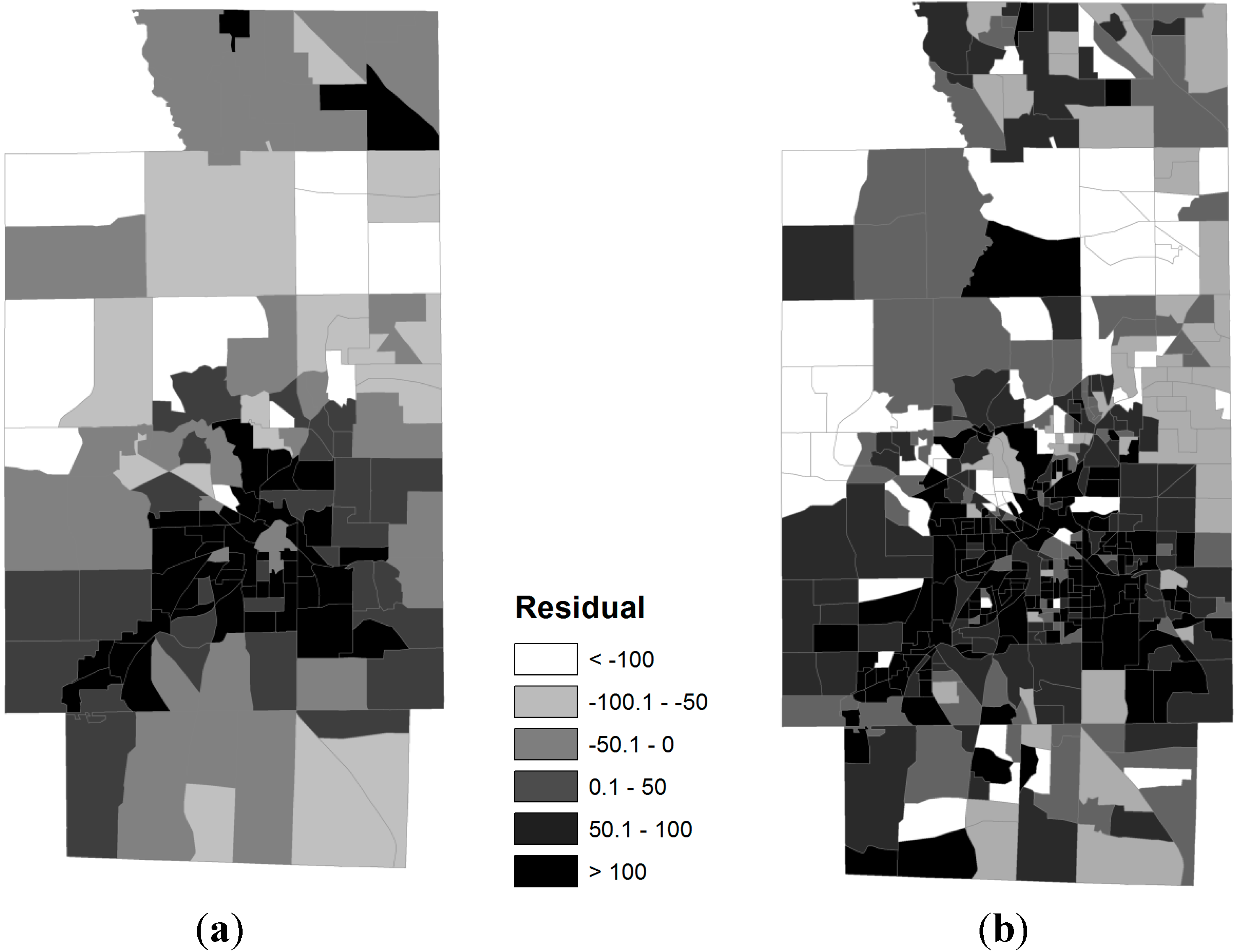
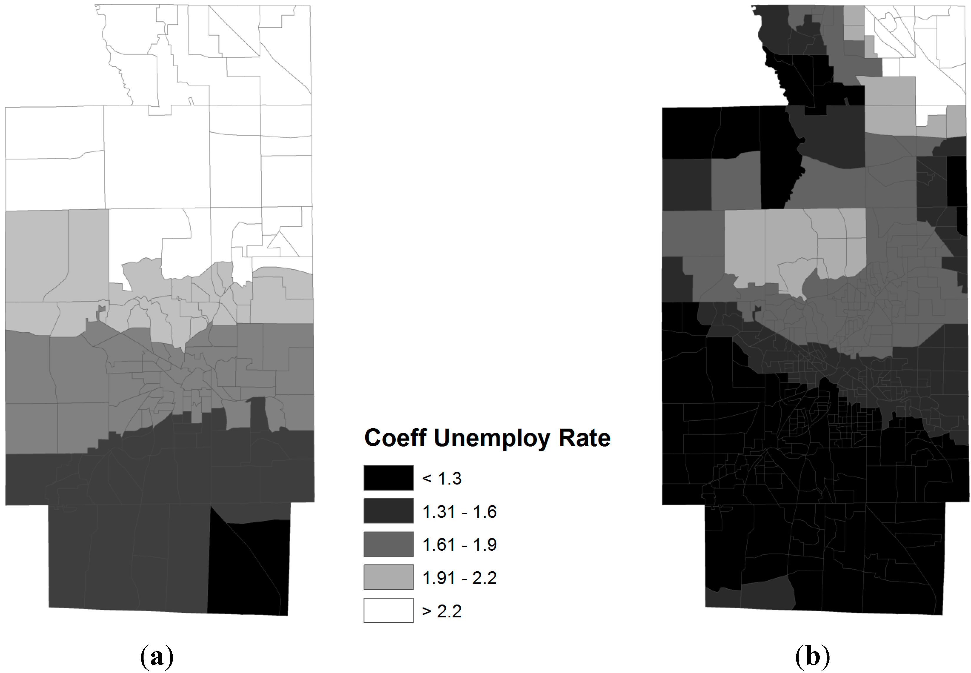
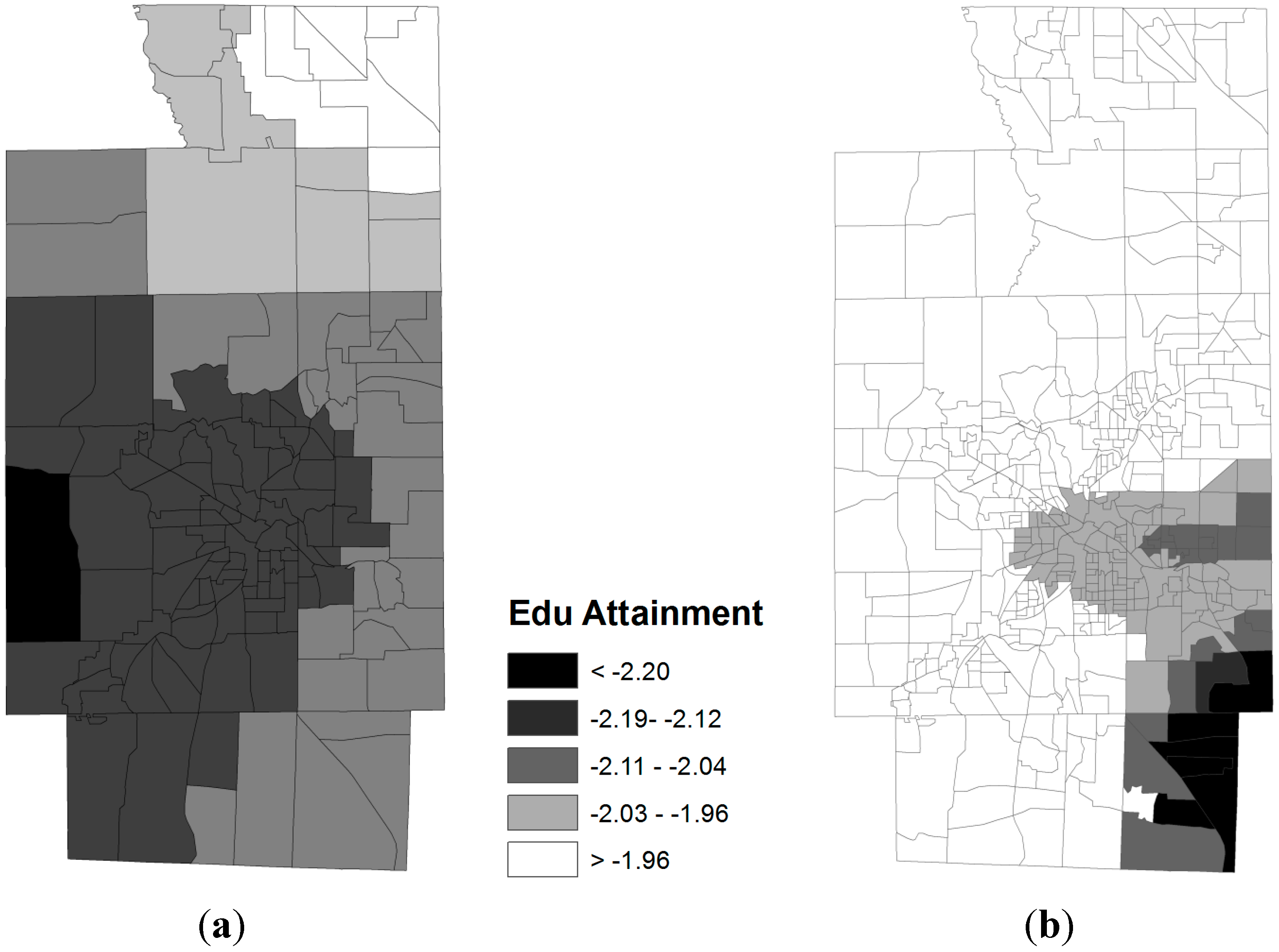
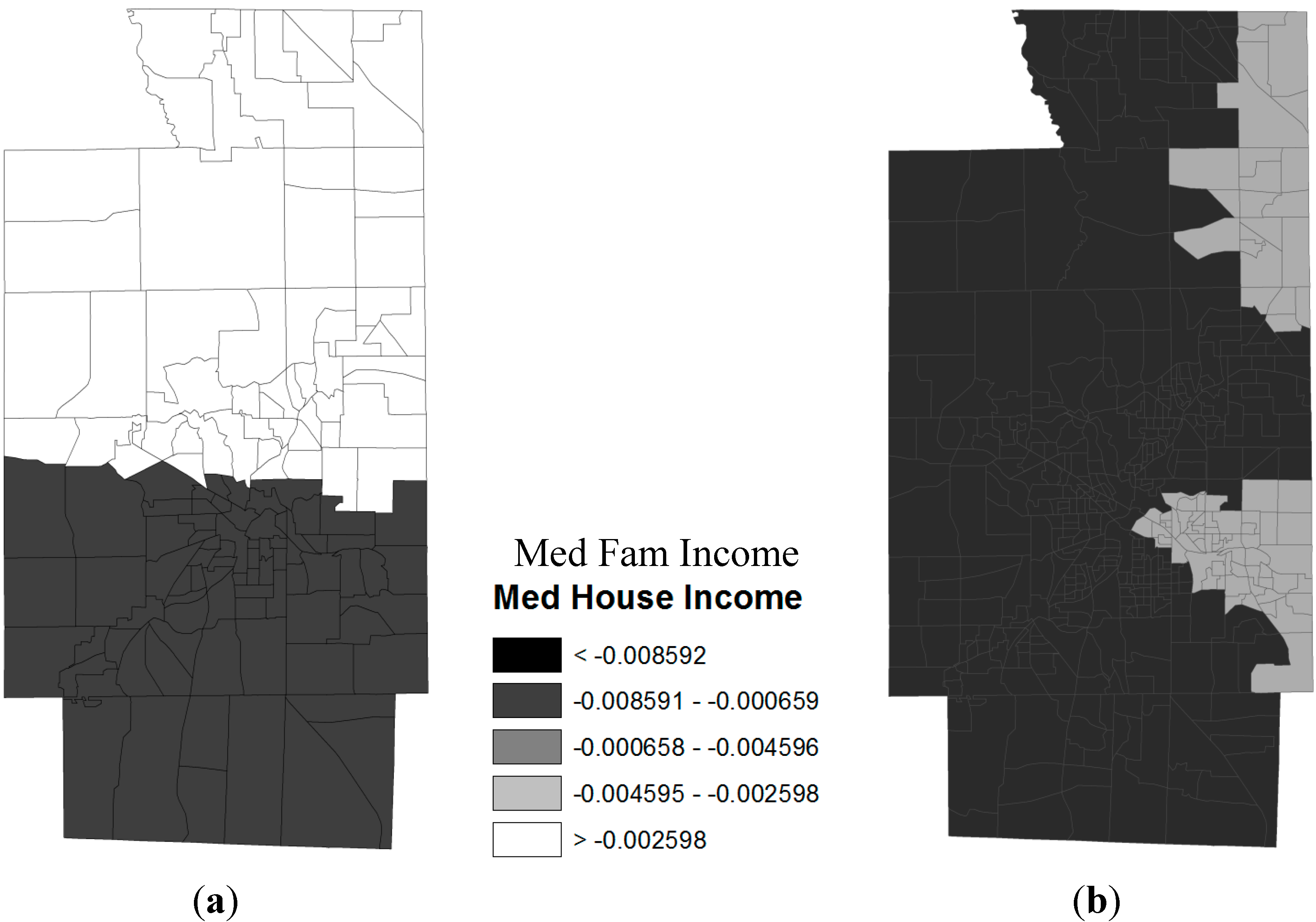
3.2. Spatial Relationships between Obese Population and SES Attributes

To examine the socio-economic and geographical disparities of the obese population, we analyzed the spatial relationships between obesity ratios and a set of carefully selected socio-economic (SES) attributes, using both census tracts and census block groups. As suggested in Geographies of Obesity [24], the socio-economic attributes that may influence obesity ratio include population density, racial composition, educational attainment, income level, employment level, and other factors. Based on these, we have assembled data from the 2011 American Community Survey (US Census Bureau) for both census tracts and census block groups with the following variables for our analysis:
  • Population density (POPDEN)
  • Percent white population (RWHITE)
  • Median family income (MEDINC)
  • Percent with bachelor degree or higher (RGEBA)
  • Percent unemployed (RUNEMP)
Using these areal attributes as explanatory (or independent) variables and obesity rates as the dependent variable, we first explored to what degrees the variations in obesity rates at both block groups (BGs) and tracts (TRs) levels can be explained by each of the independent variables. The results showed that only three variables are statistically significant in explaining the variation of obesity rates at both geographical levels. These variables are education (RGEBA), income (MEDINC), and unemployment (RUNEMP), as shown in Table 1. Lower educational attainment, lower income level, and higher unemployment ratios appear to be important in influencing the geographic patterns of obesity prevalence. It is also worth noting that the race variable was not significant. The adjusted-R2 values listed in Table 1 indicate that these regression models are relatively weak. However, it appears that these SES variables can explain the variation in obesity rates better at the tract level than at the block group level.
Table 1. Regression models with the highest adjusted-R2 values.
Adj-R2Regression Model
Bgroups0.40−RGEBA
0.41−MEDINC
0.36+RUNEMP
Tracts0.66−RGEBA
0.65−MEDINC
0.62+RUNEMP
Higher correlation coefficients are expected for larger areal units (TRs vs. BGs), as this is part of the scale effect under the MAUP, and has been well documented and explained [25]. In short, more aggregated data have less variation and smaller variance (and standard deviation). Lower in variance (and standard deviation) will partly raise the correlation. Even at the TRs level, the R2 values are not strong. One possible reason for low explanatory power of a regression model is the presence of spatial heterogeneity. While the model may have captured the pertinent variables to explain the outcomes, the relationships between the outcome and explanatory variables may vary across different observations. Such variation often follows certain geographical patterns. To address this issue, we used geographically weighted regression (GWR) [26,27] with the three explanatory variables at both the block groups and tracts levels. The results are listed in Table 2, together with results from models of ordinary least squares regression (OLS) with the same dependent and independent variables. We used ArcGIS 10.1 [28] to perform the calculations for GWR models.
Table 2. Summary output from geographically weighted regression (GWR) and ordinary least squares regression (OLS).
Obesity_Ratio = Function ( RGEBA, MEDINC, RUNEMP)
GWRR2Adjusted-R2AICc
Block Groups0.49370.46505101.32
Tracts0.73010.70701395.61
OLSR2Adjusted-R2AICc
Block Groups0.44150.43785114.80
Tracts0.69680.68991400.02
From Table 2, it can be seen that the overall adjusted-R2 value is higher at tracts level than at block groups level (1.9 fold). Again, the larger R2 value at the tract level is expected due to scale effect as in the case of ordinary regressions. In addition, AICc values are lower at the tracts level than at the block groups level. This is true for both GWR and OLS, with only minor differences in adjusted-R2 and in AICc. The performance statistics of these two models suggest that the OLS model is reasonably competent as compared to the local model using GWR because the AICc values of the OLS model are smaller than that of the GWR model. However, we will demonstrate below that despite the guidance of these model statistics favors the global OLS model, the local model has tremendous values in revealing pertinent relationships that OLS models do not reveal.
GWR essentially uses a pre-defined function to determine the level of influence that neighboring units have on each geographic unit in the regression model. For example, for census block group, bi, a pre-defined function may be based on the distance decay concept so that block groups located farther away from bi are weighted less in the regression outcomes than the immediate neighboring block groups of bi. The pre-defined function can be adjusted to reflect particular phenomena based on their spatial patterns.
Normally, the pre-defined function is applied to all geographical units. When this is the case, it is said to be using a fixed kernel. An option in using GWR to analyze spatial relationships is to vary the pre-defined function according to the density of data points locally. In areas where the data are spatially denser, the distance decay can be structured to reflect that in areas where the data are spatially less dense. When using the varying distance functions, it is said to be using adaptive kernels. In this study, we used adaptive kernel approach in our GWR models to reflect the uneven geographic distribution of the model variables.
Below in Figure 2, the distribution of residuals, i.e., the differences between actual obesity rates and the predicted obesity rates by the GWR models, shows no spatial autocorrelation in either TRs or BGs. Global Moran’s Index values, a widely used index for measuring spatial autocorrelation, is 0.016 (Z-score = −0.3737, Prob = 0.7086) for TRs and is 0.004 (Z-score = 0.1667, Prob = 0.8675) for BGs, both are not statistically significant at α = 0.025 level. The map by census tracts shows a more generalized pattern than that by census block groups. On the map by block groups, we can easily identify areas where such residuals are larger or smaller with much detail. The different levels of details as displayed by tracts and block groups suggest that smaller geographic units may be better for modeling SES and area disparities in health. Some small areas of concern may be hidden at the tract level, but are exposed at the block group level.
From the geographically weighted regression model, it is possible to observe how a particular explanatory variable influences obesity rates more or less across the study area. This is done by mapping the regression coefficients of the explanatory variables. Figure 3 shows the distribution of coefficient values for unemployment ratios in the model. It appears that the northern parts of the county experienced increased obesity rates with increased unemployment ratios where the southern and southeastern parts of the county shows the opposite trends. Again, results from using block groups do show more spatial details than what tracts reveal. However, an important aspect of these results is that unemployment and obesity levels have opposite relationships in different parts of the region (the coefficient ranges from 0.2 to 0.4), a situation that is difficult to explain, but cannot be revealed by the global regression model.
Also showing the spatial patterns of coefficient values, Figure 4 suggests that educational attainment (percent of population with bachelor degrees or higher) has a stronger impact on lowering obesity rates in the northern parts than other parts of the county. This trend is better described with block groups than with census tracts because it is much generalized in the tracts. In the City of Akron, educational attainment makes less impact on obesity rates than in the northern part of the county.
Figure 2. Spatial patterns of residuals from geographically weighted regression models, ObRates = function (RGEBA, MEDINC, RUNEMP). (a) Census Tracts, (b) Census Block Groups.
Ijgi 03 01198 g002
Figure 3. Spatial patterns of regression coefficients for unemployment ratios. (a) Census Tracts; (b) Census Block Groups.
Ijgi 03 01198 g003
Figure 4. Spatial patterns of regression coefficients for educational attainment. (a) Census Tracts; (b) Census Block Groups.
Ijgi 03 01198 g004
Again in Figure 5, which shows regression coefficients for median family income in the GWR model, tracts also generalize the spatial pattern of how median family income influences obesity rates in Summit County. With block groups, the different levels of impacts on obesity rates by median family income are shown by circular rings that center at the City of Akron—from a positive influence of increasing median family income causing slight increases of obesity rates to a negative influence of increasing median family income causing reductions in obesity rates. Comparing what are shown by tracts and by block groups, the influences by median family income on obesity rates do show significantly different patterns on the western parts of the county. In addition, similar to the unemployment variable, the coefficient value ranges from 0.2 to 0.1, indicating that the direction of the relationship is not uniform across the region. In other words, lower income level is related to lower obesity rate in some areas (center and the east), but is related to higher obesity rate in other areas (north and west).
Overall, our analysis showed that obesity rates are indeed affected by education attainment, income level, and unemployment level. While such relationships are all statistically significant for the three SES variables included in GWR models, it is important to explore in more spatial details to appreciate where inside the county we can expect such relationships to be stronger or weaker. Thus, when making policies on how to promote health and how to allocate funding to different areas in the county, for example, at neighborhood level, geographic disparities in health can be incorporated for more effective outcomes.
Figure 5. Spatial patterns of regression coefficients for median family income ($1000’s). (a) Census Tracts; (b) Census Block Groups
Ijgi 03 01198 g005

4. Discussion and Concluding Remarks

We have presented in this paper our analysis of obesity rates in terms of their spatial patterns and their relationships to a set of selected socio-economic variables. Similar analytical procedures were repeated for census tracts and census block groups to show that geographic resolutions do indeed matter in such analysis.
While individual records for adults age 16 and 21 in Summit County, Ohio, as obtained from Ohio Bureau of Motor Vehicles, were used in our study, it should be noted that this is not a 100% coverage of all adult population in Summit County—this data set does not include those who chose not to acquire driver’s licenses and those who failed to renew licenses. Furthermore, it is possible that heights and weights obtained from self-reporting through driver’s license registrations are not accurate. For example, a person’s height and weight at age 16 when first acquiring his/her driver’s license may be lower than his/her height and weight by age 20 before having to renew the license. This is a well-documented phenomenon (for example, see [23]). However, BMI data as derived from heights and weights reported to the Bureau of Motor Vehicles are probably the best and the most complete data we can obtain. If more precise analysis is in order, adjustments should be made to correct such under-reported bias.
Geographic resolutions do make a difference. In general, the higher the resolution, the more details are revealed in the results of analysis. Analysis with data at lower geographic resolution may run into the risk of obscuring potentially meaningful and informative processes operational only at the finer scale. To that end, please see Lam [29] for a discussion on different types of scale and their effects on geographic studies. As a general rule of thumb, higher resolution analyses are preferred. Unfortunately, the geographic resolution of analysis is often dictated by the availability of supporting data. Although, in this study, data at the block group level were available and used, and these data are of higher resolution than the corresponding census tract data, we need to also take into account the quality of data in addition to the desirable levels of scale or resolution. If data at different geographic resolution are of similar quality, it would be preferred to use those with more geographic details. It should also be noted here that, as more micro data (e.g., individual addresses or GPS coordinates, etc.) are increasingly available, we argue that analyses should be performed at the highest geographic resolution whenever possible and when the supporting data allow.
In our specific case, and probably our situation is also applicable to many studies in social sciences and public health, we have to used ACS data, the only major source of data in the U.S. after 2000 census in order to obtain SES information of the social environment in which the subjects resided. An important aspect of ACS data is the survey nature such that estimates, especially for smaller geographical units, tend to be unreliable, often with relatively large margin of error [30].
As we prefer to conduct analysis with data of higher geographic resolution, and therefore using block group data is preferable to reveal detailed geographical patterns, ACS data at block group level have substantially larger error than their corresponding tract level data. Just take the median family income variable as an example, the minimum, maximum, and average coefficient of variation (CV) of the variable are reported in Table 3 below. Clearly, the ACS estimates at the tract level are much more reliable than those at the block group level. In fact, some of the estimates at the block group level have their 90% margin of errors larger than the estimates. On the other hand, the quality of tract level estimates is not ideal. Nonetheless, these tract estimates are more reliable. Thus, from the data quality perspective, the tract level analysis we conducted and reported here probably offer results with a higher level of confidence. This higher confidence level, unfortunately, has to be trade-off with a lower geographical resolution in the analysis results.
Table 3. Summary of statistics of the coefficient of variation (CV) for the variable median family income from ACS at the census block groups and tracts levels.
Statistics for CVBlock Group LevelTract Level
Minimum0.01370.0250
Maximum2.25720.8192
Average0.27030.1305
Many obesity studies adopted census tracts as the de facto geographic unit of analysis. This may be due to the obvious reasons of data availability and limits to computational resources. We argue that census tracts may generalize spatial patterns too much and that census block groups or smaller geographic units should be used whenever possible. Assuming equal in data quality, analyzing geographies of obesity at a finer geographic scale enables better decisions when formulating policies to promote health for areas with health disparities.
The use of GWR also reveals new details in terms of spatial trends of how independent variables are associated with dependent variables. These spatial trends cannot be uncovered by conventional global regression models, such as ordinary least squares regression that provides only global trends of the relationships between dependent and independent variables. For example, the varying spatial trends of how unemployment ratios impact obesity prevalence as shown in Figure 3 would never be discovered using only conventional regression modeling approaches.

Author Contributions

Jay Lee contributes to the work reported in this paper with the formulation of research questions, design of analytical methods, and the writing of initial drafts. Mohammad Alnasrallah is responsible for data management and analysis and the creation of maps in this paper. David Wong extends this paper by adding the discussion on modifiable area unit problems and data quality issues. Heather Beaird provides access to data used in this research and advises the interpretation of analytic outcomes. Everett Logue assists this project with the design of the conceptual framework used in the analysis.

Conflicts of Interest

The authors declare no conflict of interest.

References

  1. Wong, D. The modifiable areal unit problem (MAUP). In The SAGE Handbook of Spatial Analysis; Fotheringham, A.S., Rogerson, P.A., Eds.; Sage: London, UK, 2009; pp. 105–123. [Google Scholar]
  2. Cockings, S.; Martin, D. Zone design for environment and health studies using pre-aggregated data. Soc. Sci. Med. 2005, 60, 2729–2742. [Google Scholar] [PubMed]
  3. Anderson, B.; Rafferty, A.P.; Lyon-Callo, S.; Fussman, C.; Imes, G. Fast-food consumption and obesity among Michigan adults. Prev. Chronic Dis. 2011, 8, A71. [Google Scholar] [PubMed]
  4. Fine, L.J.; Philogene, G.S.; Gramling, R.; Coups, E.J.; Sinha, S. Prevalence of multiple chronic disease risk factors: 2001 National Health Interview Survey. Am. J. Prev. Med. 2004, 27, 18–24. [Google Scholar] [PubMed]
  5. Flegal, K.M.; Carroll, M.D.; Ogden, C.; Johnson, C.L. Prevalence and tends in obesity among US adults, 1999–2000. J. Am. Med. Assoc. 2002, 288, 1723–1727. [Google Scholar]
  6. Hedley, A.A.; Ogden, C.L.; Johnson, C.L.; Carroll, M.D.; Curtin, L.R.; Flegal, K.M. Prevalence of overweight and obesity among US children, adolescents, and adults, 1999–2002. J. Am. Med. Assoc. 2004, 291, 2847–2850. [Google Scholar]
  7. Ogden, C.L.; Flegal, K.M.; Carroll, M.D.; Johnson, C.L. Prevalence and trends in overweight among US children and adolescents, 1999–2000. J. Am. Med. Assoc. 2002, 288, 1728–1732. [Google Scholar]
  8. Ogden, C.L.; Carroll, M.D.; Kit, B.K.; Flegal, K.M. Prevalence of obesity and trends in body mass index among US children and adolescents, 1999–2010. J. Am. Med. Assoc. 2012, 307, 483–490. [Google Scholar] [CrossRef]
  9. Flynn, M.A.T.; McNeil, D.A.; Maloff, B.; Mutasingwa, D.; Wu, M.; Ford, C.; Tough, S.C. Reducing obesity and related chronic disease risk in children and youth: A synthesis of evidence with “best practice” recommendations. Obes. Rev. 2006, 7, 7–66. [Google Scholar] [CrossRef] [PubMed]
  10. Must, A.; Spadano, J.; Coakley, E.H.; Field, A.E.; Colditz, G.; Dietz, W.H. The disease burden associated with overweight and obesity. J. Am. Med. Assoc. 1999, 282, 1523–1529. [Google Scholar]
  11. Rippe, J.M.; Crossley, S.; Ringer, R. Obesity as a chronic disease: Modern medical and lifestyle management. J. Am. Diet. Assoc. 1998, 98, S9–S15. [Google Scholar] [PubMed]
  12. Wang, Y.; Mi, J.; Shan, X.-Y.; Wang, Q.J.; Ge, K.-Y. Is China facing an obesity epidemic and the consequences? The trends in obesity and chronic disease in China. Int. J. Obes. 2007, 31, 177–188. [Google Scholar]
  13. World Health Organization. Obesity: Preventing and Managing the Global Epidemic. Available online: http://libdoc.who.int/trs/WHO_TRS_984.pdf (accessed on 24 November 2013).
  14. Eckel, R.H.; Krauss, R.M. American Heart Association call to action: Obesity as a major risk factor for coronary heart disease. Circulation 1998, 98, 2099–2100. [Google Scholar] [PubMed]
  15. Martinez, J.A. Body-weight regulation: Causes of obesity. Proc. Nutr. Soc. 2000, 59, 337–345. [Google Scholar] [CrossRef] [PubMed]
  16. Obe, C.W. Causes of obesity. In Obesity and Weight Management in Primary Care; Waine, C., Ed.; Blackwell Science: Oxford, UK, 2008; p. 118. [Google Scholar]
  17. Sonya, A.G.; Mensinger, G.; Huang, S.H.; Kumanyika, S.K.; Stettler, N. Fast-food marketing and children’s fast-food consumption: Exploring parents’ influences in an ethnically diverse sample. J. Public Policy Mark. 2007, 26, 221–235. [Google Scholar]
  18. Wilding, J. Causes of obesity. Pract. Diabetes Int. 2001, 18. [Google Scholar] [CrossRef]
  19. Wright, S.M.; Aronne, L.J. Causes of obesity. Abdom. Imaging 2012, 37, 730–732. [Google Scholar] [CrossRef] [PubMed]
  20. Sobal, J.; Stunkard, A.J. Socioeconomic status and obesity: A review of literature. Psychol. Bull. 1989, 105, 260–275. [Google Scholar] [PubMed]
  21. Zhang, Q.; Wang, Y. Trends in the association between obesity and socioeconomic status in US adults: 1971–2000. Obes. Res. 2004, 12, 1622–1632. [Google Scholar] [PubMed]
  22. McLaren, L. Socioeconomic status and obesity. Epidemiol. Rev. 2007, 29, 29–48. [Google Scholar] [CrossRef] [PubMed]
  23. Ossiander, E.M.; Emanuel, I.; O’Brian, W.; Malone, K. Driver’s license as a source of data on height and weight. Econ. Hum. Biol. 2004, 2, 219–227. [Google Scholar] [CrossRef] [PubMed]
  24. Pearce, J.; Witten, K. Geographies of Obesity: Environmental Understandings of the Obesity Epidemic; Ashgate Publishing Ltd.: Burlinton, VT, USA, 2010; p. 331. [Google Scholar]
  25. Fotheringham, A.S.; Wong, D.W.S. The modifiable areal unit problem in multivariate statistical analysis. Environ. Plan. A 1991, 23, 1025–1044. [Google Scholar] [CrossRef]
  26. Brunsdon, C.; Fotheringham, A.S.; Charlton, M. Geographically weighted regression. J. R. Stat. Soc. Ser. D 1998, 47, 431–443. [Google Scholar] [CrossRef]
  27. Fotheringham, A.S.; Brunsdon, C.; Charlton, M. Geographically Weighted Regression: The Analysis of Spatially Varying Relationships; Wiley & Sons: New York, NY, USA, 2002. [Google Scholar]
  28. ESRI. Available online: http://www.esri.com (accessed on 10 October 2014).
  29. Lam, N.S.-N. Fractals and scale in environmental assessment and monitoring. In Scale and Geographic Inquiry: Nature, Society and Method; Sheppard, E., McMaster, R.B., Eds.; John Wiley and Sons: New York, NY, USA, 2008; pp. 23–40. [Google Scholar]
  30. Sun, M.; Wong, D.W.S. Incorporating data quality information in mapping the American Community Survey data. Cartogr. Geogr. Inf. Sci. 2010, 37, 285–300. [Google Scholar]

