Article

Investigating Within-Field Variability of Rice from High Resolution Satellite Imagery in Qixing Farm County, Northeast China

1
Institute of Geography, University of Cologne, Cologne 50923, Germany
2
International Center for Agro-Informatics and Sustainable Development (ICASD), Cologne 50923, Germany
3
Geography Department, Minnesota State University, Mankato, MN 56001, USA
4
College of Resources and Environmental Sciences, China Agricultural University, Beijing 100193, China
*
Author to whom correspondence should be addressed.
ISPRS Int. J. Geo-Inf. 2015, 4(1), 236-261; https://0-doi-org.brum.beds.ac.uk/10.3390/ijgi4010236
Submission received: 3 September 2014 / Revised: 7 November 2014 / Accepted: 7 January 2015 / Published: 3 February 2015

Abstract

:
Rice is a primary staple food for the world population and there is a strong need to map its cultivation area and monitor its crop status on regional scales. This study was conducted in the Qixing Farm County of the Sanjiang Plain, Northeast China. First, the rice cultivation areas were identified by integrating the remote sensing (RS) classification maps from three dates and the Geographic Information System (GIS) data obtained from a local agency. Specifically, three FORMOSAT-2 (FS-2) images captured during the growing season in 2009 and a GIS topographic map were combined using a knowledge-based classification method. A highly accurate classification map (overall accuracy = 91.6%) was generated based on this Multi-Data-Approach (MDA). Secondly, measured agronomic variables that include biomass, leaf area index (LAI), plant nitrogen (N) concentration and plant N uptake were correlated with the date-specific FS-2 image spectra using stepwise multiple linear regression models. The best model validation results with a relative error (RE) of 8.9% were found in the biomass regression model at the phenological stage of heading. The best index of agreement (IA) value of 0.85 with an RE of 13.6% was found in the LAI model, also at the heading stage. For plant N uptake estimation, the most accurate model was again achieved at the heading stage with an RE of 11% and an IA value of 0.77; however, for plant N concentration estimation, the model performance was best at the booting stage. Finally, the regression models were applied to the identified rice areas to map the within-field variability of the four agronomic variables at different growth stages for the Qixing Farm County. The results provide detailed spatial information on the within-field variability on a regional scale, which is critical for effective field management in precision agriculture.

1. Introduction

Rice (Oryza sativa L.) is one of the most important staple food crops, feeding over half of the world’s population. In 2010, the global rice production was approximately 672 million tons from a cultivation area of around 154 million ha, with China contributing to 29% and 19% of the rice production and cultivation area, respectively [1]. Paddy rice management and its irrigation strategy have significant effects on greenhouse gas emissions [2,3]. Globally, rice paddies contribute about 10% of the total methane flux to the atmosphere [4]. In 2000, the soil nitrogen (N), phosphorus (P), and Potassium (K) nutrient deficit induced by rice production accounted for 42% of the global deficit amount [5]. Paddy rice agriculture in China is therefore of national and global significance in terms of both food security and sustainable development.
In the past years, remote sensing (RS) as an advanced technology has been used extensively in agriculture to obtain spatial and temporal information about crops [6,7,8,9]. Paddy rice areas were well projected using RS techniques [10,11,12]. Geographic Information System (GIS) data have been proved to be important to enhance the accuracy of land use and land cover classification [13,14]. RS data with coarse and medium resolution are widely used in rice cultivation research [12,15,16,17,18,19,20,21,22,23,24,25,26]. However, the number of conducted studies on rice using high resolution RS images was limited in the past two decades [23,27,28]. Identification of rice cultivation areas and estimation of agronomic parameters from high resolution images are valuable for improving rice production.
Mapping rice cultivation areas accurately is fundamental for the assessment of agricultural and environmental productivities, the analysis of food security and therefore national and international food trade decisions [29,30,31]. Many previous studies have mapped rice areas [12]. Various classifiers, including maximum likelihood, artificial neural network, decision tree, and spatial reclassification kernel, have been used in vegetation mapping using RS. However, classification accuracies are mainly determined by the quality and quantity of RS data. No ideal image classifier is uniformly applicable to all tasks [32]. Extensive field knowledge and auxiliary data help to improve the classification accuracy [32]. In the Multi-Data-Approach (MDA) for land use and land cover classifications as well as crop rotation mapping, multi-temporal RS and GIS vector data are combined to derive as much information as possible. Studies [16,17] demonstrated that considering extensive field knowledge and ancillary GIS data in the post-classification process can improve the classification accuracy by up to 10%.
Agricultural RS refers to the method of non-contact measurements of electromagnetic radiation reflected or emitted from plant materials or soils in agricultural fields [33]. Different vegetative covers can be distinguished according to their unique spectral behavior in relation to overall ground elements [34]: Visible radiation in the red (630–690 nm) is absorbed by chlorophyll while radiation in the near infrared (760–900 nm) is strongly reflected by leaf cellular structures. Vegetation Indices (VIs) are developed to qualitatively and quantitatively evaluate vegetative characteristics by combining spectral measurements from different wavelength channels [35]. Theoretically, the VIs should be particularly sensitive to vegetative covers, insensitive to non-vegetation factors such as soil properties, atmospheric effects and sensor viewing conditions [36]. In practice, factors of soil characteristics, atmosphere and sensor radiometry degradation, as well as differences in the spectral responses and bidirectional effects all have considerable effects on vegetation indices. Therefore, many VIs have been developed to enhance the vegetative cover signal while minimizing the background response [35]. Hansen and Schjoerting [37] discussed the optimized NDVI from different band centers and band widths to represent wheat parameters such as biomass, leaf area index (LAI), chlorophyll, and N status. In their study, the partial least square regression algorithm was applied. Yao et al. [38] successfully explored empirical models based on ground-based RS techniques to estimate N status and improve N use efficiency in rice. Yu et al. [39] investigated the potential of hyperspectral band combinations in interpreting canopy N status in rice. Despite the lack of interpretations of the physical mechanisms and interactions between the target properties and the measured signals, these empirical models are fundamental materials for further research in order to represent the physical reality.
Remotely sensed photosynthetically active radiation has been used to evaluate the primary production of crops [40,41]. The most sophisticated method commonly combines RS data with dynamic crop growth models [42,43]. However, these methods require numeric parameters and are sensitive to soil background conditions.
Precision agriculture (PA) emerged in the middle of the 1980s [33]. Later, in 1991, satellite data were firstly used in PA [44]. Spatial and temporal variability of soil and crop factors within a field is the essential base of PA [45]. Measurement of various crop canopy variables during the growing season provides an opportunity for improving grain yield and quality by site-specific fertilizer applications. Due to the ability of providing high temporal, spatial and spectral resolution images, satellite RS has a significant potential in PA [33,46]. The multi-temporal within-field information on crop status captured by satellite RS is invaluable in PA.
Because of its operational and economical uses over large areas, satellite RS technology has been widely used to conduct in-season crop yield forecasting for decision making on marketing intervention and policy support on regional or global scales [29,31]. Satellite RS is also an essential technique for agro-ecosystem studies on regional scales [47,48,49].
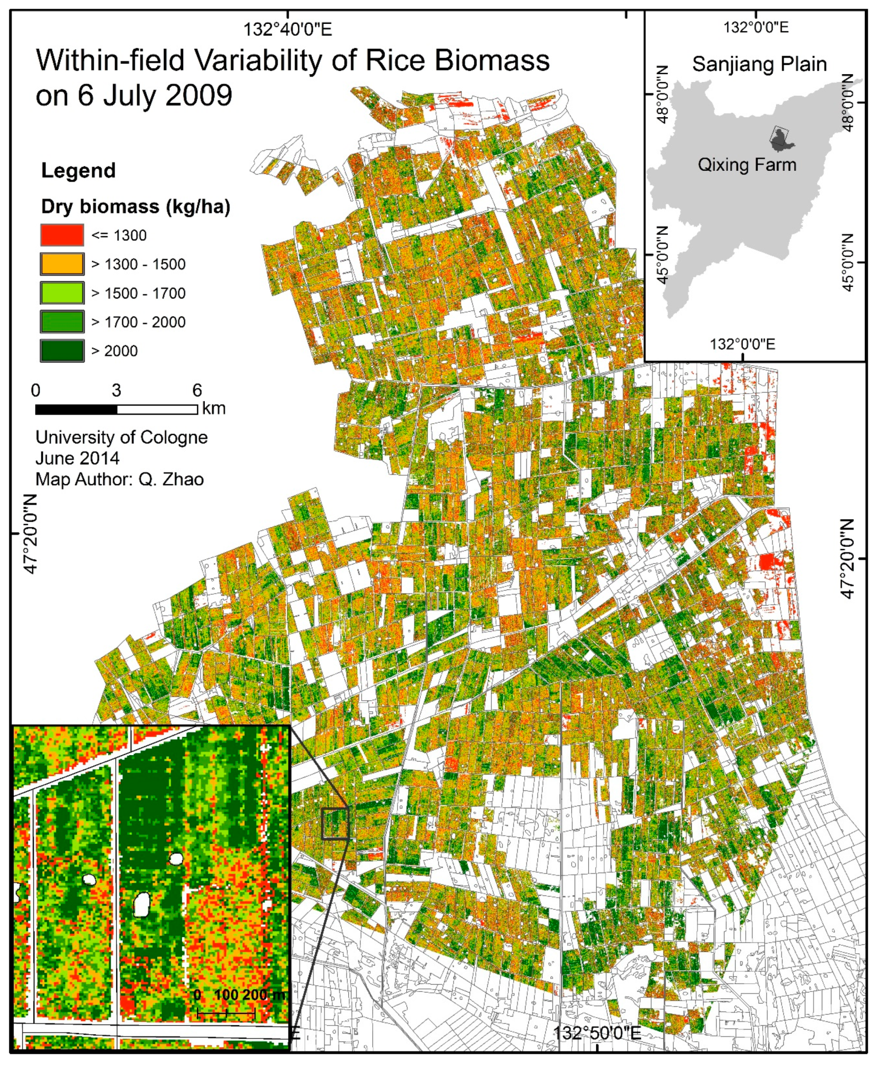
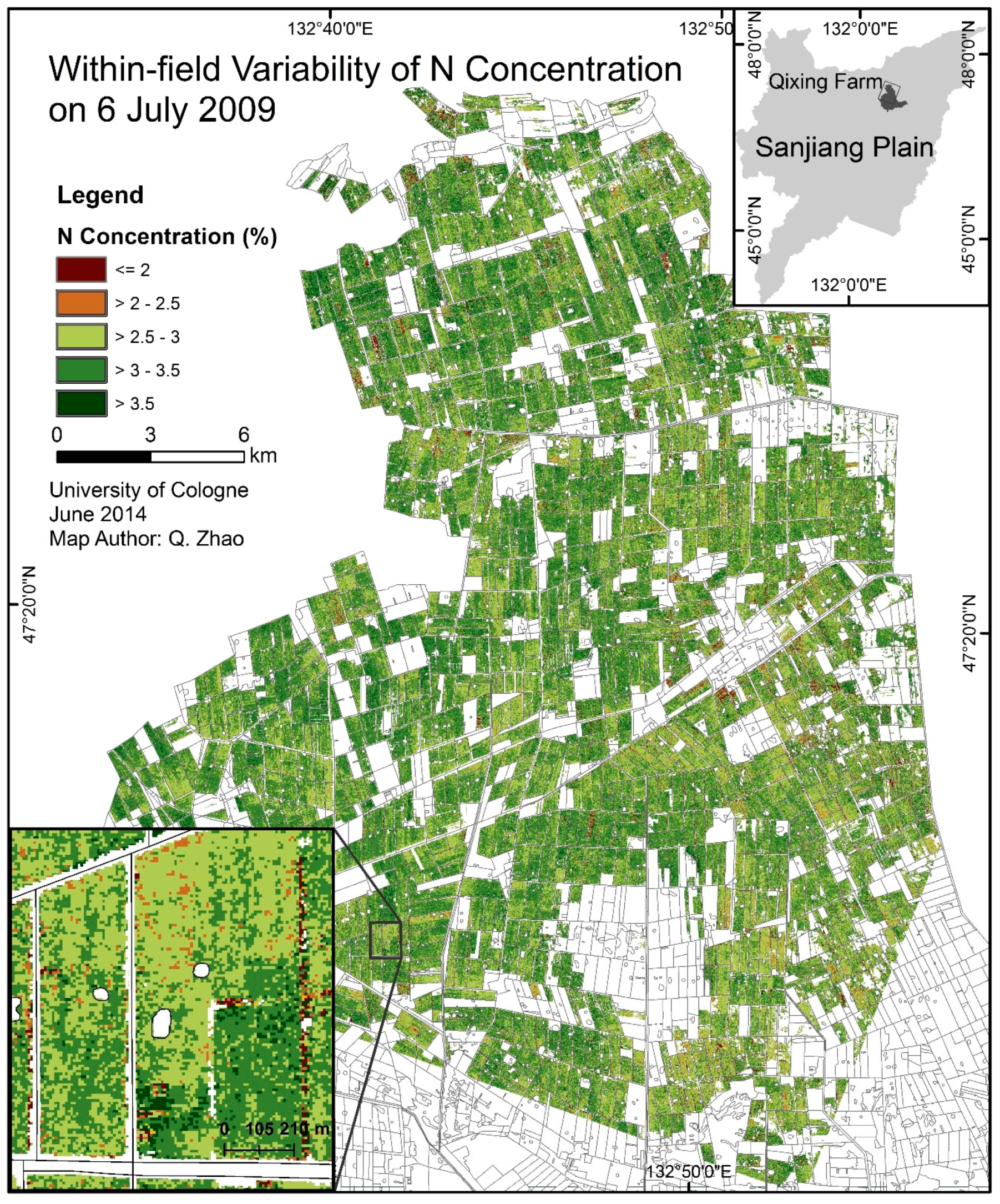
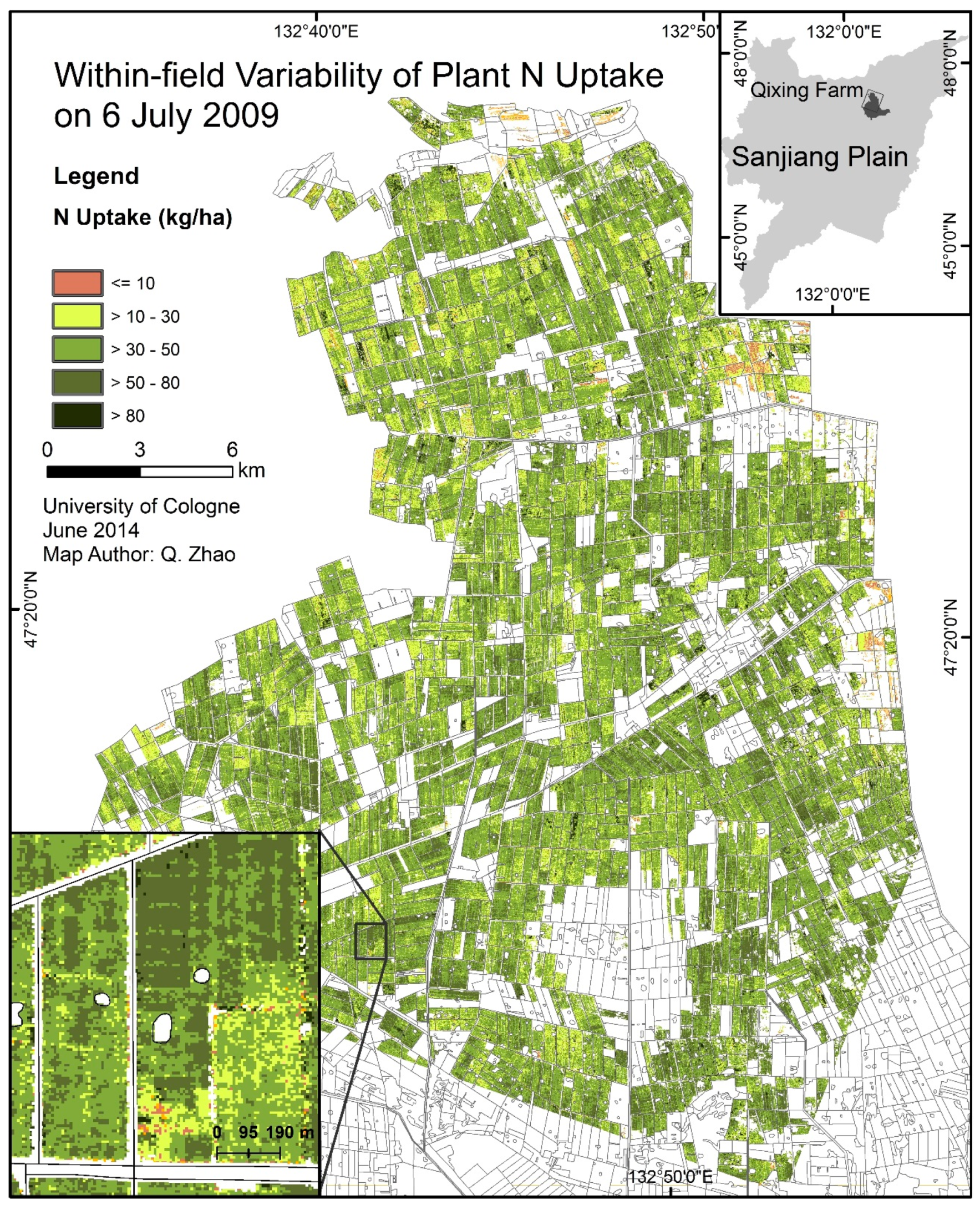
The overall aim of this study is to investigate the possibilities and accuracies of within-field variability of rice status monitoring during the entire growing season on a county scale (Qixing Farm) using satellite RS data. The term “within-field variability” in this study refers to the spatial variability of agronomic variables (biomass, LAI, N concentration, N uptake, etc.) within a rice crop field defined by enclosed boundaries. The size of a rice field in this study ranges from 0.5–100 ha. First, a map of rice cultivation areas was produced using multi-temporal RS FORMOSAT-2 (FS-2) images, coupled with auxiliary GIS data (MDA) to improve the classification accuracy. Then, empirical regression models were developed to relate RS spectra with field measurements of the four agronomic variables. One advantage of this research is the construction of specific regression models for different growth stages. Based on a stepwise regression analysis, the optimized predictors from the satellite images were identified to investigate the dynamics of crop canopy characteristics at different stages. The specific objectives of this study are to (1) identify rice cultivation areas with high classification accuracies based on multi-temporal RS and GIS data; (2) develop regression models for deriving rice crop variables from the FS-2 imagery; (3) validate the ability of the regression models to estimate rice parameters; (4) apply the regression models to the entire Qixing Farm County study area.
The presented method of extracting high resolution within-field variability information from the FS-2 imagery will assist farmers in their site-specific rice crop management and strategy planning.

2. Study Area

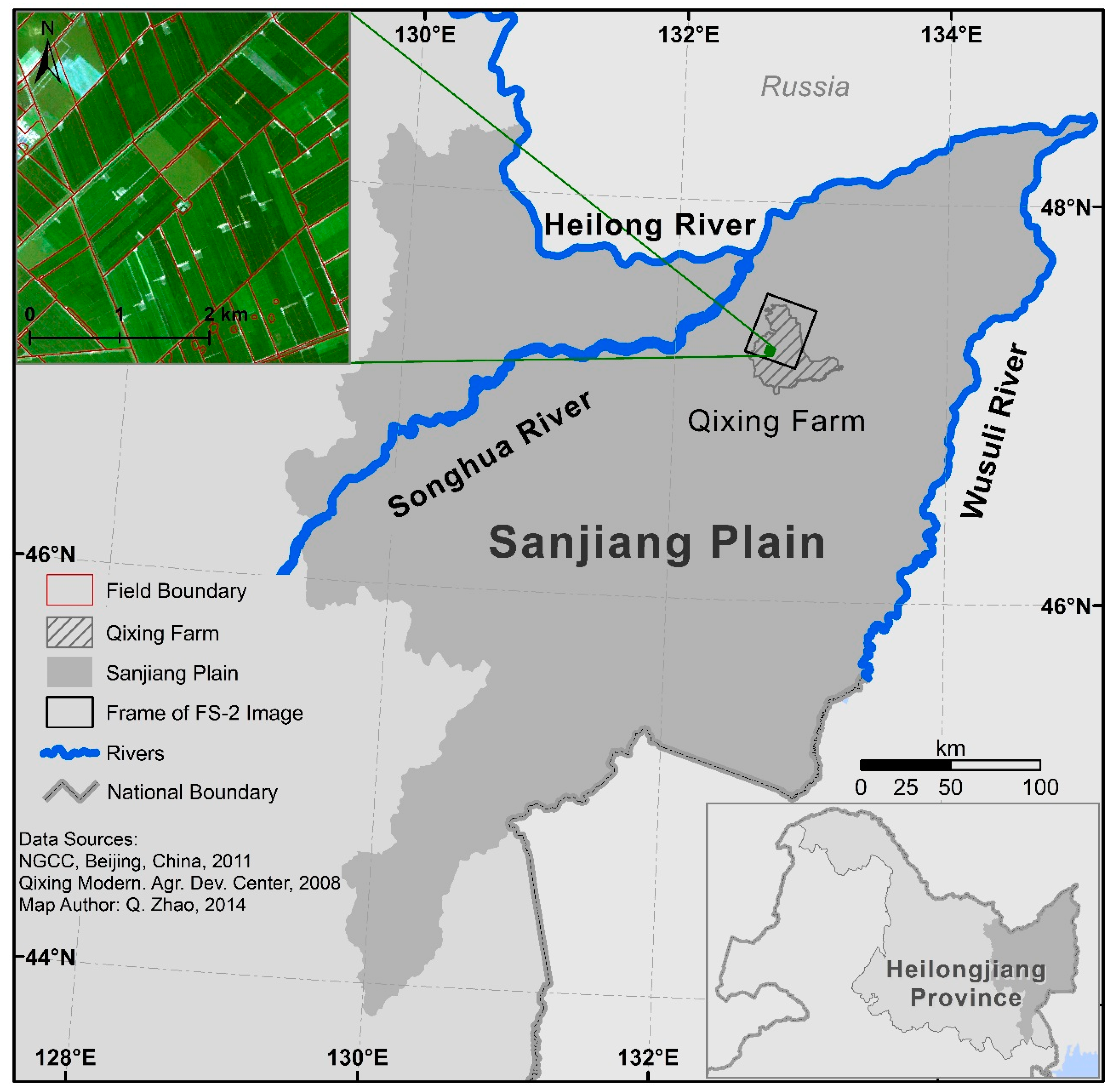
The study site Qixing Farm (47.2°N, 132.8°E), is located in the Sanjiang Plain (SJP) in North-eastern China (see Figure 1). The SJP is an alluvial plain formed by the Songhua River, the Heilong River and the Wusuli River. The administrative area of the Qixing Farm County is about 120,000 ha. The climate in the SJP is temperate sub-humid, with a mean annual precipitation of 500–650 mm. Rainfall mainly occurs from May to September during the growing season of crops. The accumulated ≥ 10 °C temperature all across the year is about 2300–2500 °C and only single-season crops are planted. The topography is rather flat with an average elevation of 60 m and is characterized by broad alluvial plains and low terraces formed by the rivers. The SJP, which covers an area of more than 100,000 km2, exceeding the size of the Netherlands almost by three times, is one of the major agricultural areas of China. In 2009, arable land in the SJP accounted for nearly 60% of the total land, being dominated by paddy rice (57%) [50]. Since the irrigation constructions (water channels, raised ridges) for paddy rice are reusable year by year, the field boundaries are mostly stable. In recent years, for better economic profit, there has been moderate land use change from dryland to paddy rice. Compared with Europe’s highly fragmented agricultural landscapes which prevent the utility of coarse resolution RS data for quantitative crop monitoring and yield forecasting [32], SJP’s large homogenous landscapes provide an ideal site for monitoring crops using satellite RS.
Figure 1. Location of the study area in Northeast China (the upper left corner shows a subset of the FS-2 image acquired on 9 August 2009).
Ijgi 04 00236 g001

3. Data

3.1. Satellite RS Images and GIS Data

FORMOSAT-2 (FS-2) collects multispectral images with a ground pixel resolution of 8 × 8 m2 over a swath of 24 km. The FS-2 images used in this study are optical images with 4 bands of blue (450–520 nm), green (520–600 nm), red (630–690 nm), and near-infrared (760–900 nm). Three tiles of high quality images covering the main arable land area (~56,000 ha) of the Qixing Farm were captured on 24 June, 6 July, and 9 August, in 2009. Thus, both the vegetative phase (24 June and 6 July) and the reproductive phase (9 August) of rice are well represented in these images.
GIS vector data of Qixing Farm field boundaries were provided by the Qixing Modern Agriculture Research Center. Information on crop field boundaries, irrigation wells, water drainages, and shelter forests edges are given at a fine field unit scale. Additional information such as crop type of each field is given in the GIS attribute table.

3.2. Ground Truth Data Collection

Field campaigns for the agronomic data collection were carried out during the entire rice growing season in 2009. In total, 42 sample sites covered by the FS-2 images were selected for this study. All these 42 sites were located in seven farmers’ fields being spatially separated. Each site was represented by one plot covering approximately 0.1–0.3 ha. The final plant samples collected from each site were a mixture of three or four spatially separated samples, taken from the same plot. As ground truth data, the areas of sample sites were mapped using a Trimble™ Global Positioning System (GPS) receiver. Field management calendars of transplanting, N topdressing, irrigation, application of insecticides, and harvest dates, were recorded. Several field campaigns were carried out to collect samples from the tillering stage, booting stage, heading stage, 20 days after heading, and the harvest stage. For each site, biomass, LAI and plant N concentration were measured and plant N uptake was calculated as well.
After the field sampling, the plants were first cleaned, and then separated into different organs (leaves, stems, panicles) to measure the biomass values. LAI was measured using a sub-sample of the leaf biomass. One sub-sample consisted of 10–20 leaves, randomly selected among the youngest fully developed leaves. All fresh samples were processed in the oven at 105 °C for half an hour to stop enzyme activity. After that, they were dried at 75 °C for at least 72 h until a constant weight was reached before they were finally weighted. N concentration was measured using the Kjeldahl-N method. The plant N uptake was calculated as the aboveground dry mass multiplied by the N concentration. Detailed information is listed in Table 1.
In the study area, rice cultivation technologies in high latitude are relatively sophisticated and rice cultivation regulations developed by the government are applied by most of the farmers. The rice seedlings are first grown in greenhouses and are then transplanted into the paddy fields. In the regulations, a date window of 15–25 May is suggested for transplanting in order to capture the maximum accumulated temperature throughout the whole year. In this research, we divided our ground truth data sets into two groups according to the transplanting dates. Sample sites with seedlings transplanted from 15–25 May were used to construct empirical regression models between the agronomic parameters and the RS data. Sample sites with seedlings transplanted beyond those dates were used as validation data sets to evaluate the performance of the regression models.
Table 1. Agronomic parameters of the sample sites in 2009.
FieldNumber of Sample SitesVarietyNumber of FoliageTransplanting DateQuantity of N Topdressing (kg/ha)Plant Density (plants/m2)Soil Properties
pHK (mg/kg)P (mg/kg)N (mg/kg)SOM (g/kg)
Field 14Longjing 2112May 10104, 104, 104, 1041096.0575.726.7181.137.98
3Kongyu 13111May 170, 94, 141
1Xixuan 113May 151321016.22134.536.6177.435.47
1Longdun 10412May 16118 6.07142.530.1173.646.85
1Longjing 2112May 171181336.0882.428.3175.837.78
Field 24Longjing 2112May 1384, 84, 84, 841155.59103.833.2259.941.83
3Longjing 2112May 130, 67, 101115
Field 34Longjing 2112May 1267, 67, 67, 671176.13126.524.0209.049.52
4Longjing 2112May 120, 54, 81, 67117
Field 44Kendao 611May 2083, 83, 83, 831586.29372.521.5249.866.03
Field 54Longjing 2411May 1695, 95, 95, 951665.8473.437.8176.235.76
1Longjing 2411May 160166
Field 61Longdun 24912May 20102 5.78126.530.6169.737.08
1Chaoyou 94911May 181061446.0898.432.0187.539.91
3Jinxuan 111May 200, 86, 129
Field 73Kongyu 13111May 170, 82, 123122

4. Methods

4.1. Satellite Image Pre-Processing

Pre-processing of satellite images prior to vegetation information extraction is essential to remove noise and increase the interpretability of image data [51]. Solar radiation reflected by the earth surface to the satellite sensors is significantly affected by its interaction with the atmosphere. Atmospheric correction is an important pre-processing step for satellite RS [52,53]. The uncertainties resulting from atmospheric effects in agriculture applications of satellite RS have been well discussed during the past decades [18,21,54,55]. In this study, atmospheric correction was performed using ENVI FLAASH, version 5.1. Table 2 lists the main parameters used in the atmospheric correction process. The sub-arctic summer model for rural region was selected.
Table 2. Main atmospheric correction parameters for the FS-2 images.
DateVisibility (km)Zenith AngleAzimuth Angle
June 2450146°10′0.84″−115°13′19.56″
July 650152°15′58.34″−45°34′58.34″
August 950155°12′2.90″−83°58′22.08″
Geometric distortion is another important factor affecting the results of image processing, especially when combing geospatial data from different dates or multiple sources. Dai and Siamak [56] noted that the geometric error even on a sub-pixel level can significantly affect the accuracy of land use classification from satellite images. The precision of geometric correction depends on the number, distribution, and accuracy of the Ground Control Points (GCPs) [57]. To avoid labor intensive work of in-situ GCP collection, Zhao et al. [58] developed a geometric correction method for georeferencing multi-source geodata by using TerraSAR-X data as a reference. The same method was applied in this study. Specifically, a stacked TerraSAR-X image produced from five dates served as the reference to georectify the FS-2 images. The main georeferencing parameters are shown in Table 3. The positional error (PE) was less than 6 m for all three images. More details about the method can be found in Zhao et al. [58].
Table 3. Main georeferencing parameters for the FS-2 images.
Image Capture DateNumber of Control PointsNumber of Check PointsPE of Control Points (m)PE of Check Points (m)
June 24100202.9915.901
July 6104204.1435.032
August 9101203.3535.666
The mean reflectance and VIs for each sample plot were calculated using the “Zonal Analysis” tool in ERDAS IMAGINE 2013. For each of the three FS-2 images, correspondingly 42 RS samples were extracted and used to develop the empirical regression models for crop status monitoring.

4.2. Mapping Rice Cultivation Areas

A rice area map of the Qixing Farm in 2009 was produced using aforementioned MDA. In particular, multi-temporal RS and GIS data were integrated to improve the accuracy of rice mapping. Based on the properties/attributes of the different datasets, a knowledge base was constructed and implemented, using the Knowledge Engineering tool mounted in ERDAS IMAGINE 2013. A series of logical rules were created in the Knowledge Engineering tool to integrate the RS and GIS data in order to achieve higher classification accuracy.
The general steps for delineating rice areas are summarized as follows: (1) a supervised classification based on the maximum likelihood algorithm was carried out. In order to extract more unique spectral signatures, more than five subclasses were classified firstly (for the image of June 24: nine subclasses in total with one of them being rice; for the image of July 6: 16 subclasses in total with three of them representing rice; for the image of August 9: 11 subclasses in total with three representing rice); (2) the resulting subclasses were further combined to five main classes, including rice, dryland, forests, residential areas, and “other areas” for each image; (3) isolated pixels were eliminated using the “clump and eliminate” functions embedded in ERDAS IMAGINE 2013; (4) an expert classification system based on knowledge rules was implemented to integrate and improve the rice classification results from multiple dates; and (5) the vector GIS data were used as auxiliary dataset in the post-classification process to further improve the accuracies of rice classification.
In a MDA study, Waldhoff et al. [13] reported that the support vector machine (SVM) approach and the maximum likelihood classifier (MLC) yielded similar classification accuracies. They found although the SVM method performed slightly better (up to 3%) in three of the four cases, the MLC had a shorter processing time. Therefore, the MLC was selected in this study to derive multi-temporal high resolution land cover classifications over a large study area. After the classification, the rice classes derived from the three RS images were “combined” by logical rules to take advantage of the specific spectral information corresponding to growth stages. Specifically, in the first step of the supervised classification, to improve the producer’s accuracy of rice classes, relatively “broad” spectral information was selected as rice spectral signatures. Thus, some other land covers such as “dryland” and “bare soils” may have been classified into rice classes as well. However, these misclassified areas from one single image could be different from those areas from the other dates, because spectral differences between rice and other land covers vary with growth stage [59]. In the next step, using the knowledge base, the pixels classified into rice classes in all three RS images were categorized into a new “rice class 1”. The areas classified into rice classes in two RS images were categorized into a new “rice class 2”. After that, these refined RS rice areas were further “combined” with the GIS data (rice area masks). To assign a pixel into the final rice class, the following conditions had to be satisfied: (1) this pixel was in the “rice class 1”; or (2) this pixel was in the “rice class 2” and in the GIS rice mask.

4.3. Ground Truth Data Interpolation

Ground truth data for each site were collected at the tillering stage (28–30 June), the jointing stage (10–12 July), the heading stage (2–8 August), 20 days after heading (22–28 August), and the harvest time. The FS-2 images were acquired on 24 June, 6 July and 9 August, at slightly different dates from the field campaigns. Therefore, the values of the agronomic variables of biomass, LAI, plant N concentration and N uptake were interpolated for these three FS-2 dates. First, a specific polynomial growing curve for each site was constructed based on the time series of ground truth data. The values of the agronomic variables for the three RS-2 dates were then interpolated. These interpolated values were used as the new ground truth data to explore their relationships with the satellite image reflectance and VIs.

4.4. Development of Regression Models for Deriving Agronomic Variables

A multiple linear regression method was constructed for each agronomic variable based on reflectance values and the VI derived from the FS-2 images and the corresponding field measurement. The VI used in this method was treated as an equivalent factor of reflectance. Correlation and regression analyses were performed in SPSS 21 (SPSS, Inc., Chicago, IL, USA). The format of the multiple linear regression models was as follows:
Y E = α 0 + α B l u e   × R B l u e   + α G r e e n   × R G r e e n   + α R e d   × R R e d   + α N I R   × R N I R   + α N D V I   × N D V I
The NDVI is calculated by the following function:
N D V I = ( R N I R R R e d ) / ( R N I R + R R e d )  
R stands for the reflectance value at the subscripted satellite band. In Equation (1), YE stands for the estimated agronomic variable; α i is the coefficient of the reflectance at the corresponding band/vegetation index. The performance of the regression model was evaluated by the coefficient of determination (R2).
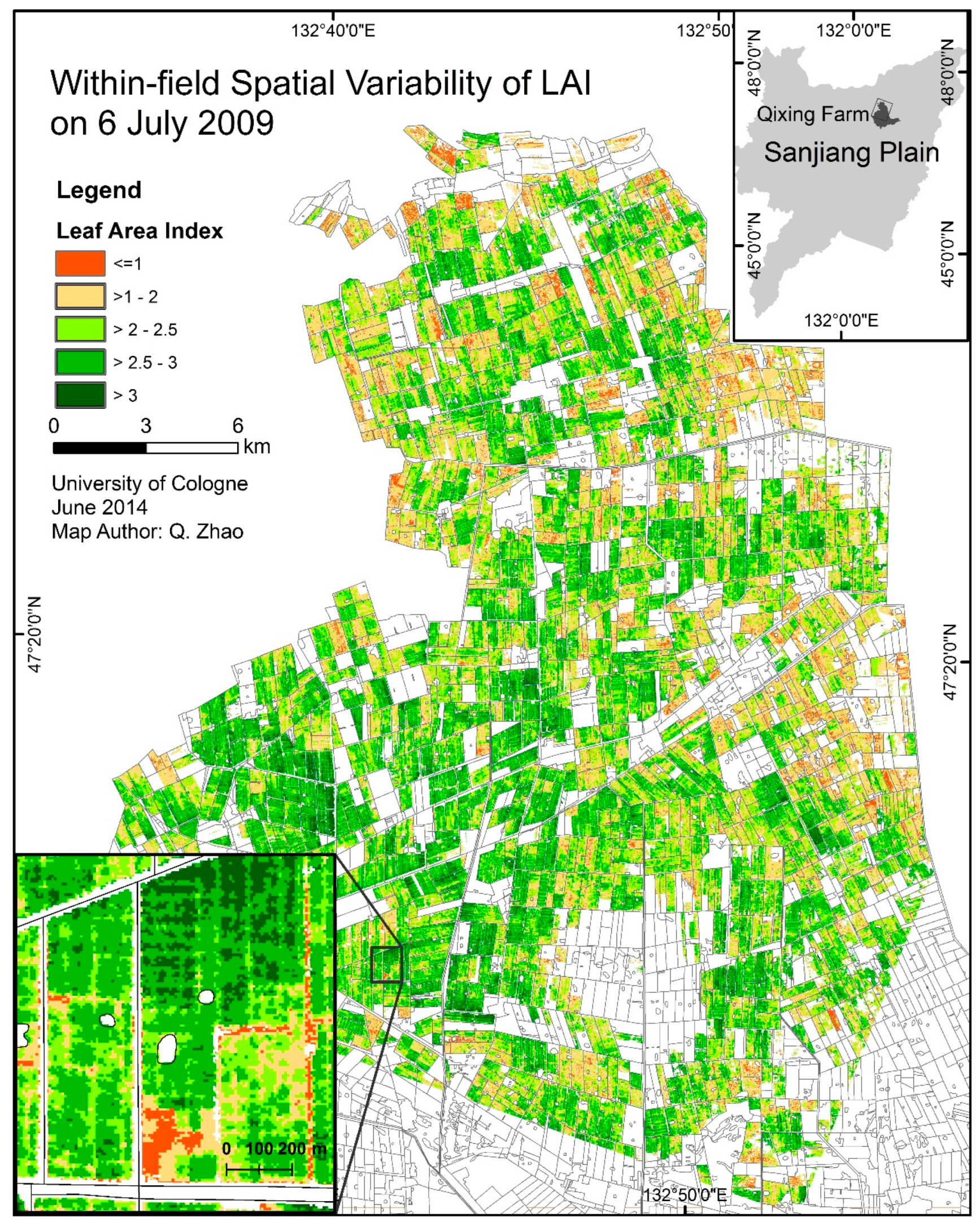
Biomass and LAI are essential crop physiological variables which determine the crop yield. LAI refers to the ratio of leaf surface area to ground area. It is a fundamental canopy parameter in agronomy and RS since it drives absorption of solar radiation and evapotranspiration for carbon assimilation, and thus primary production. In this research, both biomass and LAI were related to the FS-2 band reflectance based on the aforementioned Equation (1).
N is one of the most remobilizable elements during the reproductive stage in rice plants [60]. Since its remobilization causes leaf senescence, it is directly related to crop productivity [61]. Accurate plant N status detection to develop site specific N management strategies for rice in the SJP is of importance regarding both agricultural and environmental aspects [39]. In this study, plant N concentration and N uptake were also derived from the FS-2 images using the regression model represented by Equation (1).

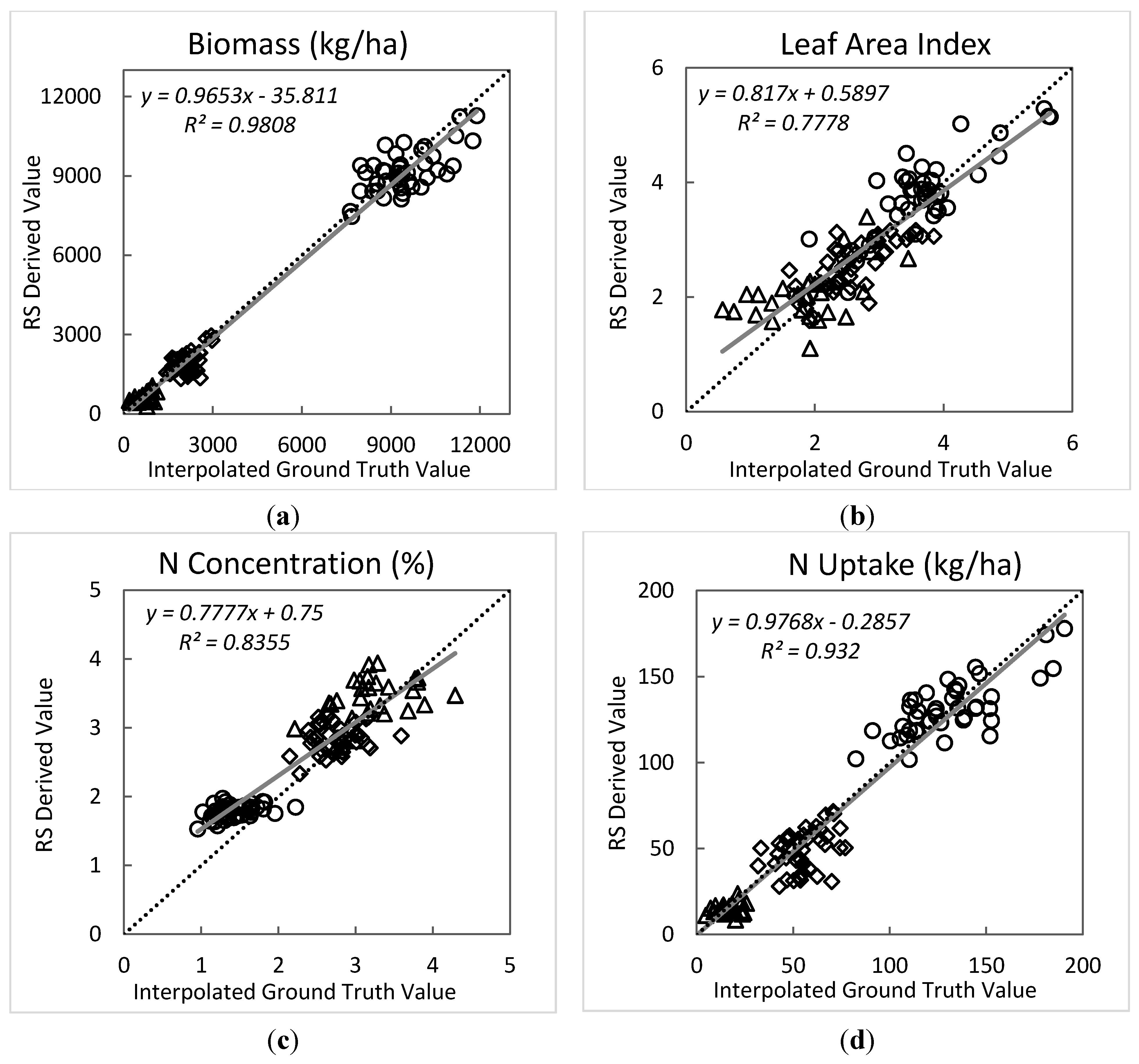
4.5. Validation of the Regression Models

The regression models were evaluated in a validation analysis. The feasibility of the model was quantified by the statistical measures of relative error (RE) and index of agreement (IA). In a further step, scatterplots were generated to assess the performance of the regression models. The RE is the ratio of the Root Mean Square Error (RMSE) to the mean of observed values, describing the differences between the predicted and the observed values relative to the mean of the ground truth values. The IA represents the degree of agreement between the model estimations and observed values [62]. It is calculated as:
I A = 1 i = 1 n ( O i P i ) 2 / i = 1 n ( | P i O ¯ | + | O i O ¯ | ) 2
where O i is the observed value, P i is the model-simulated value, and O ¯ is the mean of observed values. The denominator in Equation (3) was defined as a “potential error” by Willmott [62]; therefore the IA represents the ratio between the mean square error and the “potential error”. Although the IA is sensitive to extreme values [63], it can be interpreted straightforwardly since it ranges from 0–1.

5. Results

5.1. Accuracy of Rice Area Classification

To compare the classification accuracies from different data sources, 800 random points were created in the study area. More than 80 random points were distributed in each class. Error matrices were generated to quantify the classification accuracies. The kappa coefficients of agreement and overall accuracies for the rice class are shown in Table 4.
Table 4. Accuracies of rice maps produced from different data sources.
Data SourceUser’s Accuracy of RiceProducer’s Accuracy of RiceKappa CoefficientOverall Accuracy
RS single date (August 9)94.1%82.6%0.73380.8%
RS multiple dates (3 dates)89.4%91.7%0.78185.0%
RS and GIS data combined94.2%92.7%0.88191.6%
With auxiliary GIS data, both the Kappa and the overall accuracy values for the rice class were improved by 0.148 and 10.8%, respectively. While a similar user’s accuracy was obtained after combining the three RS classification maps and the GIS ancillary data, the producer’s accuracy increased from 82.6% to 92.7%, implying a decrease of 10% in omission errors. These results are in line with the conclusions made by Shrestha and Zinck [64] and Rozenstein and Karnieli [14].

5.2. Empirical Regression Models

5.2.1. Model Development

The parameters of the best qualified regression models for all agronomic variables are shown in Table 5. The coefficient of determination R2 was used to evaluate the regression models.
Table 5. Parameters of empirical regression models.
Agronomic VariablePhenological StageNumber of Model Construction SitesRegression Model Parameters
Model CoefficientR2
α 0 α B l u e α G r e e n α R e d α N I R α N D V I
Biomass (kg/ha)Tillering17−316.063 52,440−25,250 0.551 **
Booting237280.37913,48051,620−121,53021,270−12,113.1820.765 **
Heading235791.901 −148,910 31,710 0.519 **
LAITillering17−1.04 140−50 0.458 *
Booting23−0.451 4.3780.431 **
Heading23−5.463−50−27038030 0.650 **
N Concentration (%)Tillering174.371 −101.54871.492 0.401#
Booting234.89550.798−22.079−23.972−4.718 0.269 #
Heading230.193−35.742−44.725105.143.459 0.075 #
N Uptake (kg N/ha)Tillering17−21.022−370290260140 0.273 #
Booting23−18.834810690−1420280 0.460 *
Heading23167.251 −4270 550 0.483 **
Significance test: ** p < 0.01, * p < 0.05, # p > 0.05.
A stepwise multiple linear regression was applied to select the best RS predictors for the regression models at different phenological stages.
For the biomass regression models, the best R2 values, ranging from 0.519–0.765, were achieved. At the tillering stage, only green and red bands were applied to represent the biomass; while at the booting stage, all four bands as well as the NDVI value were included in the model. At the heading stage, only green and NIR bands were used. Across all three dates, the model for the booting stage (second date), near the height of the growing season, gives the highest R2 value of 0.765.
The stepwise regression analysis for the LAI estimation chose red and green bands as the predictors in the tillering stage, NDVI as the only predicting variable in the booting stage, and all four bands as predictors in the heading stage. The LAI estimation model with the best performance was found at the heading stage when panicles grow outside of the rice stem, with an R2 of 0.65.
Variations in N concentration are more difficult to detect than biomass or LAI development. The N concentration is a weak absorber of spectral radiation and occurs in very small quantities in leaf tissue (0.5–3%) [65]. The red and green bands of the FS-2 image were included in the regression model in the tillering stage, while all four bands were used in both the booting and heading stages. At the tillering and booting stages, when the plant N concentration is at a high level, higher associations were found between the plant N concentration and the RS spectra.
Stepwise regression analysis for N uptake included all four bands as predictors in the tillering and booting stages, whereas only green and NIR were needed in the heading stage. The highest R2 was 0.483 at the heading stage.

5.2.2. Validation of the Regression Models

Model validation was conducted using independent ground truth data sets as mentioned in Section 3.2. Table 6 shows the statistics of the model validation.
Table 6. Validation results for the regression models.
Agronomic variablePhenological StageNumber of Validation SitesModel Validation Parameter
RE (%)IA
Biomass (kg/ha)Tillering1239.40.38
Booting1927.00.32
Heading198.90.68
LAITillering1231.40.38
Booting1715.10.60
Heading1713.60.85
N Concentration (%)Tillering1217.70.41
Booting1915.30.48
Heading1927.70.48
N uptake (kg N/ha)Tillering1239.90.39
Booting1932.50.37
Heading1911.00.77
Validation analyses (Table 6) showed that the regression model for biomass reached the lowest RE of 8.9% and highest IA of 0.68 at the heading stage. Across all three dates, for the biomass, LAI and N uptake estimation models, the RE value decreases as rice grows. The LAI model in the heading stage showed the lowest RE and highest IA values of 13.6% and 0.85, respectively. These results demonstrated that the models based on the FS-2 images performed better at later growth stages.
The RE for the N concentration model was the lowest (15.3%) at the booting stage, while the IA values increase slightly from 0.41 at the tillering stage up to 0.48 at the later booting and heading stages. For the N uptake models, the lowest RE (11%) and the highest IA (0.77) also occurred at the heading stage.
Across all three dates, relationships between the FS-2 derived values and the interpolated ground truth data were analyzed by scatterplots (Figure 2). The R2 value was the highest (0.98) for biomass modeling results, followed by the N uptake model (0.93), whereas a moderate R2 value of 0.78 and 0.84 was achieved for LAI and plant N concentration estimation. These results showed that the RS derived values were highly related to the ground truth values, and the linear regression trend lines were ideally close to the 1:1 line (dashed diagonal lines in the figures).
Figure 2. Relationships between RS derived values and ground truth values for (a) biomass; (b) LAI; (c) N concentration; and (d) N uptake at the tillering (△), booting (◊), and heading (○) stages.
Ijgi 04 00236 g002

5.3. Regional Application of the Regression Models

Finally, the regression models were applied to the identified rice areas to map the within-field variability of the four agronomic variables for the area covered by the FS-2 images in the Qixing Farm County. As an example, the results for July 6 are shown in Figure 3, Figure 4, Figure 5 and Figure 6. The within-field variability of the rice status can be easily detected in these maps. In the biomass map (Figure 3), unevenly distributed values and patterns can be identified in most of the field blocks, revealing significant within-field variability of the growing status. Overall, a relatively higher biomass level is shown in the southern part.
Figure 3. Within-field spatial variability of biomass derived from the FS-2 image of 6 July 2009.
Ijgi 04 00236 g003
The LAI map (Figure 4) reveals higher LAI values in the south, especially the southwest, region of the study area. Variations within the field blocks are also well detected in this map.
Figure 4. Within-field spatial variability of LAI derived from the FS-2 image of 6 July 2009.
Ijgi 04 00236 g004
The N concentration distribution map (Figure 5) shows a general random pattern of spatial variation on the intra-field level. Most of the fields had N concentration values of 2.5–3.5%. However, the within-field variability is still presented.
Figure 5. Within-field spatial variability of N concentration derived from the FS-2 image of 6 July 2009.
Ijgi 04 00236 g005
Likewise, the N uptake map (Figure 6) displays apparent within-field spatial variation. In the south and southeast part of the image, a relatively higher plant N uptake is detected.
Figure 6. Within-field spatial variability of N uptake derived from the FS-2 image of 6 July 2009.
Ijgi 04 00236 g006

6. Discussion

6.1. Band Selection for Different Growth Stages

The recorded reflectance of optical imagery from a vegetated surface is a function of several physical properties such as vegetation structure, soil type, plant moisture content as well as sensor configuration. Plant pigments have distinct absorption spectra and some have an impact upon the reflectance spectra of leaves. This offers the opportunity of characterizing pigment concentration from reflectance spectra [66], and thus to interpret the plant status. Chlorophylls are one of the most important pigments because they control the absorption amount of solar radiation which determines the photosynthesis and, consequently, primary production. Several studies have demonstrated that the plant chlorophyll concentration indirectly indicates the plant nutrient status because the molecular structure of chlorophyll incorporates a large proportion of total leaf nitrogen [67,68,69].
In our results, different spectral bands were selected for the regression models at different growth stages. The red and green band combination performed well for most of the agronomic variables at the tillering stage, whereas green and NIR band combinations performed best for biomass and N uptake estimation at the heading stage. At the earlier growth (tillering) stage, the rice canopy coverage is lower (much less than 100%), resulting in a lower chlorophyll concentration on the pixel scale. In addition, the chlorophyll concentration on the leaf scale is lower compared to that at the heading stage [70,71]. However, at the later (heading) stage, the canopy cover is higher, and the leaf level chlorophyll concentration is higher as well. The blue band did not frequently show up in the stepwise regression models. This may be attributed to the strong scattering effects of the atmosphere on blue radiation.
In addition, we found when the plant N concentration was relatively high, green (520–600 nm) and red (630–690 nm) bands were effective for the regression models. This result conforms to the finding of O’Neill et al. [65] that the highest correlation between N concentration and reflectance occurred at 697.8 nm, followed by the region of 536.8–558.5 nm.

6.2. Background Effects in the Early Stage

According to the model validation results of REs, it can be concluded that the regression models for the tillering stage did not perform as well as the ones for the other two stages, regarding all agronomic variables except for N concentration. The highest RE of N concentration occurred at the heading stage, which mainly was caused by the low N concentration in leaf tissue at that stage, as mentioned in Section 5.2.1.
According to the IA, the regression models performed best in the heading stage for all agronomic variables, probably resulting from the higher biomass density and thus lower field soil and water effects compared to the early stages. This result is in conflict with the findings of Gnyp et al. [72], who utilized hyperspectral field data for rice biomass estimation and achieved better results at the early growth stages. However, in the study of Gnyp et al. [72], a specific vegetation index such as NDVI or RVI (ratio vegetation index) was used as the single independent variable in the regression models. They reported that NDVI became saturated at later growth stages before biomass reached 3 t/ha, which might have affected the model performance. They also noted that at the heading stage, the canopy reflectance signal became more complicated since panicles emerged from the sheath. In this study, the original multi-spectral reflectances in addition to NDVI were both used as the descriptive variables in the stepwise regression, which might help to remove the effects of the NDVI saturation problem on the model performance at later growth stages. Nevertheless, this needs to be further confirmed by analyzing the datasets from the two studies. Additionally, different measurement methods, RS instruments, physical conditions of the rice crop, sun angles, and sensor view angles, may also contribute to the discrepancy in these two studies.
In vegetation studies using satellite RS, several caveats have been noted by Myneni et al. [73]. These caveats include bidirectional effects, atmospheric effects, canopy structure effects, background or soil effects, nonlinear effects of scattering, effects of spectral heterogeneity, adjacent effects, nonlinear mixing, and topographic effects. In this study, the background soil and water effects and the rice canopy structure significantly affect the spectral response. Canopy conditions at different stages are clearly represented in the following photos (Figure 7). At the early stage, the rice canopy coverage was relatively low and therefore more soil and water background effects occurred. As one of the important canopy structure parameters, leaf orientation characterized by a smaller leaf angle at the early stage might result in the weak performance of the regression models as well.
Figure 7. Rice growth on 24 June (left), 6 July (middle) and 9 August (right).
Ijgi 04 00236 g007

7. Conclusions

Due to the integration of multi-temporal FS-2 imagery and GIS data, the rice cultivation areas in the Qixing Farm County were more clearly identified. The overall accuracy of the entire classified map was improved remarkably from 81.8% to 91.6%. This highly accurate rice cultivation map provides an ideal basis for further analyses of rice crops in the study area.
This study showed that the performance of the regression models was significantly affected by rice growth stages. Thus, an optimized band selection for every growth stage is important due to the varying spectral reflectance properties. Based on the R2 values, relatively higher goodness-of-fit values were found in the biomass and LAI estimation models than in the plant N uptake and plant N concentration models. In particular, for the estimation of plant N concentration, better model goodness-of-fit occurred at the earliest growth stage (tillering) when the N concentration was relatively high. The RS derived values and the interpolated ground truth values for all three dates were highly correlated. The most accurate models with the lowest REs and the highest IA values were found at the heading stage for three of the four agronomic variables, except for the N concentration. In conclusion, this study provides a framework and example of how high resolution satellite RS can support agricultural field management such as fertilizer, irrigation and pesticides management strategies by providing within-field agronomic information on regional scales. The information derived from satellite RS could be further used to study the relations between crop growth and other phenomena such as carbon fixation, climate change, and sustainable management of natural resources.

Acknowledgments

This work was funded by the Natural Science Foundation of China (NSFC, project No. 31071859), the International Bureau of the German Federal Ministry of Education and Research (BMBF, project No. 1DO12013), and the German Research Foundation (DFG, project no. BA 2062/8-1). The authors gratefully acknowledge Yinkun Yao, Shanyu Huang, Minmin Su and Guangming Zhao from the China Agriculture University; Martin Gnyp and Christoph Hütt from the University of Cologne; Liqin Zhao from the Qixing Modern Agriculture Development Center for their supports in ground truth data collection. The authors are extremely thankful to the cooperating officers and farmers for their assistance in field experiments at the Qixing Farm. The Qixing Research and Development Center and the Jiansanjiang Agricultural Research Station, both in Heilongjiang, China, are gratefully acknowledged. The leading author is supported by the China Scholarship Council (November 2010–October 2014), Beijing, China.

Author Contributions

Quanying Zhao conducted the field campaigns, processed and analyzed the satellite images and the agronomic data. She also was responsible for writing the manuscript and incooperating the co-authors’ contributions and comments. Victoria Lenz-Wiedemann and Fei Yuan intensively contributed to the writing of the manuscript and the data analysis. Rongfeng Jiang, Yuxin Miao and Fusuo Zhang designed and supervised the field campaigns, and contributed to the agronomic data analysis and those parts in the manuscripts. Georg Bareth intensively contributed to the structure of the manuscript, the GIS analysis and the satellite image classification. At different stages of the analysis and writing process, all co-authors contributed ideas for the preparation and improvement of the paper.

Conflicts of Interest

The authors declare no conflict of interest.

References

  1. Food and Agriculture Organization of the United Nations. FAO Statistical Database. Available online: http://www.fao.org/docrep/015/i2490e/i2490e03d.pdf (accessed on 13 June 2014).
  2. Yan, X.; Ohara, T.; Akimoto, H. Development of region-specific emission factors and estimation of methane emission from rice fields in the East, Southeast and South Asian countries. Glob. Change Biol. 2003, 9, 237–254. [Google Scholar] [CrossRef]
  3. Smith, P.; Martino, D.; Cai, Z.; Gwary, D.; Janzen, H.; Kumar, P.; McCarl, B.; Ogle, S.; O’Mara, F.; Rice, C.; et al. Greenhouse gas mitigation in agriculture. Philos. Trans. R. Soc. B 2008, 363, 789–813. [Google Scholar] [CrossRef]
  4. Global Methane Initiative. Global Methane Emissions and Mitigation Opportunities. Available online: http://www.globalmethane.org (accessed on 26 August 2014).
  5. Tan, Z.X.; Lal, R.; Wiebe, K.D. Global soil nutrient depletion and yield reduction. J. Sustain. Agr. 2005, 26, 123–146. [Google Scholar] [CrossRef]
  6. Kumar, M.; Monteith, J.L. Remote sensing of crop growth. In Plants and the Daylight Spectrum; Smith, H., Ed.; Academic Press: London, UK, 1981; pp. 133–144. [Google Scholar]
  7. Moulin, S.; Bondeau, A.; Delecolle, R. Combining agricultural crop models and satellite observations: From field to regional scales. Int. J. Remote Sens. 1998, 19, 1021–1036. [Google Scholar] [CrossRef]
  8. Hatfield, J.L.; Gitelson, A.A.; Schepers, J.S.; Walthall, C.L. Application of spectral remote sensing for agronomic decisions. Agron. J. 2008, 100, S117–S131. [Google Scholar] [CrossRef]
  9. Gitelson, A.A.; Peng, Y.; Arkebauer, T.J.; Schepers, J. Relationships between gross primary production, green LAI, and canopy chlorophyll content in maize: Implications for remote sensing of primary production. Remote Sens. Environ. 2014, 144, 65–72. [Google Scholar] [CrossRef]
  10. Frolking, S.; Qiu, J.; Boles, S.; Xiao, X.; Liu, J.; Zhuang, Y.; Li, C.; Qin, X. Combining remote sensing and ground census data to develop new maps of the distribution of rice agriculture in China. Glob. Biogeochem. Cycle 2002, 16. [Google Scholar] [CrossRef]
  11. Xiao, X.; Boles, S.; Liu, J.; Zhuang, D.; Frolking, S.; Li, C.; Salas, W.; Moore, B., III. Mapping paddy rice agriculture in southern China using multi-temporal MODIS images. Remote Sens. Environ. 2005, 95, 480–492. [Google Scholar] [CrossRef]
  12. Kuenzer, C.; Knauer, K. Remote sensing of rice crop areas. Int. J. Remote Sens. 2013, 34, 2101–2139. [Google Scholar] [CrossRef]
  13. Waldhoff, G.; Curdt, C.; Hoffmeister, D.; Bareth, G. Analysis of multitemporal and multisensor remote sensing data for crop rotation mapping. In Proceedings of the 2012 International Archives of the Photogrammetry, Remote Sensing and Spatial Information Sciences, Melbourne, Australia, 25 August–1 September 2012; pp. 177–182.
  14. Rozenstein, O.; Karnieli, A. Comparison of methods for land-use classification incorporating remote sensing and GIS inputs. Appl. Geogr. 2011, 31, 533–544. [Google Scholar] [CrossRef]
  15. Chang, K.; Shen, Y.; Lo, J. Predicting rice yield using canopy reflectance measured at booting stage. Agron. J. 2005, 97, 872–878. [Google Scholar] [CrossRef]
  16. Wang, Y.; Chang, K.; Chen, R.; Lo, J.; Shen, Y. Large-area rice yield forecasting using satellite imageries. Int. J. Appl. Earth Obs. 2010, 12, 27–35. [Google Scholar] [CrossRef]
  17. Van Niel, T.G.; McVicar, T.R. Current and potential uses of optical remote sensing in rice-based irrigation systems: A review. Crop Pasture Sci. 2004, 55, 155–185. [Google Scholar] [CrossRef]
  18. Duggin, M.J.; Piwinski, D. Recorded radiance indices for vegetation monitoring using NOAA AVHRR data; atmospheric and other effects in multitemporal data sets. Appl. Opt. 1984, 23, 2620–2623. [Google Scholar] [CrossRef] [PubMed]
  19. McCloy, K.R.; Smith, F.R.; Robinson, M.R. Monitoring rice areas using LANDSAT MSS data. Int. J. Remote Sens. 1987, 8, 741–749. [Google Scholar] [CrossRef]
  20. Okamoto, K.; Yamakawa, S.; Kawashima, H. Estimation of flood damage to rice production in North Korea in 1995. Int. J. Remote Sens. 1998, 19, 365–371. [Google Scholar] [CrossRef]
  21. Che, N.; Price, J.C. Survey of radiometric calibration results and methods for visible and near infrared channels of NOAA-7, -9, and -11 AVHRRs. Remote Sens. Environ. 1992, 41, 19–27. [Google Scholar] [CrossRef]
  22. Fang, H.; Wu, B.; Liu, H.; Huang, X. Using NOAA AVHRR and Landsat TM to estimate rice area year-by-year. Int. J. Remote Sens. 1998, 19, 521–525. [Google Scholar] [CrossRef]
  23. Kim, H.O.; Yeom, J.M. Multi-temporal spectral analysis of rice fields in South Korea using MODIS and RapidEye satellite imagery. J. Astron. Space Sci. 2012, 29, 407–411. [Google Scholar] [CrossRef]
  24. Son, N.T.; Chen, C.F.; Chen, C.R.; Chang, L.Y.; Duc, H.C.; Nguyen, L.D. Prediction of rice crop yield using MODIS EVI-LAI data in the Mekong Delta, Vietnam. Int. J. Remote Sens. 2013, 34, 7275–7292. [Google Scholar] [CrossRef]
  25. Huang, J.; Wang, X.; Li, X.; Tian, H.; Pan, Z. Remotely sensed rice yield prediction using multi-temporal NDVI data derived from NOAA’s-AVHRR. PLoS One 2013, 8, e70816. [Google Scholar] [CrossRef] [PubMed]
  26. Peng, D.; Huang, J.; Li, C.; Liu, L.; Huang, W.; Wang, F.; Yang, X. Modelling paddy rice yield using MODIS data. Agric. For. Meteorol. 2014, 184, 107–116. [Google Scholar] [CrossRef]
  27. Chang, C.H.; Liu, C.C.; Tseng, P.Y. Emissions inventory for rice straw open burning in Taiwan based on burned area classification and mapping using FORMOSAT-2 satellite imagery. Aerosol Air Qual. Res. 2013, 13, 474–487. [Google Scholar]
  28. Kim, H.O.; Yeom, J.M. Effect of red-edge and texture features for object-based paddy rice crop classification using RapidEye multi-spectral satellite image data. Int. J. Remote Sens. 2014, 35, 7046–7068. [Google Scholar]
  29. MacDonald, R.B.; Hall, F.G. Global crop forecasting. Science 1980, 208, 670–679. [Google Scholar] [CrossRef] [PubMed]
  30. Xiao, X.; Boles, S.; Frolking, S.; Li, C.; Babu, J.Y.; Salas, W.; Moore, B. Mapping paddy rice agriculture in South and Southeast Asia using multi-temporal MODIS images. Remote Sens. Environ. 2006, 100, 95–113. [Google Scholar] [CrossRef]
  31. Duveiller, G.; López-Lozano, R.; Seguini, L.; Bojanowski, J.S.; Baruth, B. Optical remote sensing requirements for operational crop monitoring and yield forecasting in Europe. In Proceedings of 2012 nel-3 OLCI/SLSTR and MERIS/(A) ATSR Workshop, Frascati, Italy, 15–19 October 2012.
  32. Xie, Y.; Sha, Z.; Yu, M. Remote sensing imagery in vegetation mapping: A review. J. Plant Ecol. 2008, 1, 9–23. [Google Scholar] [CrossRef]
  33. Mulla, D.J. Twenty five years of remote sensing in precision agriculture: Key advances and remaining knowledge gaps. Biosyst. Eng. 2013, 114, 358–371. [Google Scholar] [CrossRef]
  34. Tucker, C.J. Red and photographic infrared linear combinations for monitoring vegetation. Remote Sens. Environ. 1979, 8, 127–150. [Google Scholar] [CrossRef]
  35. Bannari, A.; Morin, D.; Bonn, F.; Huett, A.R. A review of vegetation indices. Remote Sens. Rev. 1995, 13, 95–120. [Google Scholar] [CrossRef]
  36. Jackson, R.D.; Slater, P.N.; Pinter, P.J., Jr. Discrimination of growth and water stress in wheat by various vegetation indices through clear and turbid atmospheres. Remote Sens. Environ. 1983, 13, 187–208. [Google Scholar] [CrossRef]
  37. Hansen, P.M.; Schjoerring, J.K. Reflectance measurement of canopy biomass and nitrogen status in wheat crops using normalized difference vegetation indices and partial least squares regression. Remote Sens. Environ. 2003, 86, 542–553. [Google Scholar] [CrossRef]
  38. Yao, Y.; Miao, Y.; Huang, S.; Gao, L.; Ma, X.; Zhao, G.; Jiang, R.; Chen, X.; Zhang, F.; Yu, K.; et al. Active canopy sensor-based precision N management strategy for rice. Agron. Sustain. Dev. 2012, 32, 925–933. [Google Scholar] [CrossRef]
  39. Yu, K.; Li, F.; Gnyp, M.L.; Miao, Y.; Bareth, G.; Chen, X. Remotely detecting canopy nitrogen concentration and uptake of paddy rice in the Northeast China Plain. ISPRS J. Photogramm. Remote Sens. 2013, 78, 102–115. [Google Scholar] [CrossRef]
  40. Hall, F.G.; Huemmrich, K.F.; Goward, S.N. Use of narrow-band spectra to estimate the fraction of absorbed photosynthetically active radiation. Remote Sens. Environ. 1990, 32, 47–54. [Google Scholar] [CrossRef]
  41. Baret, F.; Hagolle, O.; Geiger, B.; Bicheron, P.; Miras, B.; Huc, M.; Berthelot, B.; Niño, F.; Weiss, M.; Samain, O.; et al. LAI, fAPAR and fCover CYCLOPES global products derived from VEGETATION: Part 1: Principles of the algorithm. Remote Sens. Environ. 2007, 110, 275–286. [Google Scholar] [CrossRef] [Green Version]
  42. Bouman, B.A.M. Linking physical remote sensing models with crop growth simulation models, applied for sugar beet. Int. J. Remote Sens. 1992, 13, 2565–2581. [Google Scholar] [CrossRef]
  43. Prasad, A.K.; Chai, L.; Singh, R.P.; Kafatos, M. Crop yield estimation model for Iowa using remote sensing and surface parameters. Int. J. Appl. Earth Obs. 2006, 8, 26–33. [Google Scholar] [CrossRef]
  44. Bhatti, A.U.; Mulla, D.J.; Frazier, B.E. Estimation of soil properties and wheat yields on complex eroded hills using geostatistics and thematic mapper images. Remote Sens. Environ. 1991, 37, 181–191. [Google Scholar] [CrossRef]
  45. Zhang, N.; Wang, M.; Wang, N. Precision agriculture—A worldwide overview. Comput. Electron. Agr. 2002, 36, 113–132. [Google Scholar] [CrossRef]
  46. Thenkabail, P.S. Biophysical and yield information for precision farming from near-real-time and historical Landsat TM images. Int. J. Remote Sens. 2003, 24, 2879–2904. [Google Scholar] [CrossRef]
  47. Donlon, C.; Berruti, B.; Buongiorno, A.; Ferreira, M.H.; Féménias, P.; Frerick, J.; Goryl, P.; Klein, U.; Laur, H.; Mavrocordatos, C.; et al. The global monitoring for environment and security (GMES) sentinel-3 mission. Remote Sens. Environ. 2012, 120, 37–57. [Google Scholar] [CrossRef]
  48. Duveiller, G.; Baret, F.; Defourny, P. Remotely sensed green area index for winter wheat crop monitoring: 10-Year assessment at regional scale over a fragmented landscape. Agr. For. Meteorol. 2012, 166, 156–168. [Google Scholar] [CrossRef]
  49. Duveiller, G.; Defourny, P. A conceptual framework to define the spatial resolution requirements for agricultural monitoring using remote sensing. Remote Sens. Environ. 2010, 114, 2637–2650. [Google Scholar] [CrossRef]
  50. Ouyang, W.; Xu, Y.; Hao, F.; Wang, X.; Chen, S.; Lin, C. Effect of long-term agricultural cultivation and land use conversion on soil nutrient contents in the Sanjiang Plain. Catena 2013, 104, 243–250. [Google Scholar] [CrossRef]
  51. Dhaliwal, J.S.; Benbasat, I. The use and effects of knowledge-based system explanations: Theoretical foundations and a framework for empirical evaluation. Inf. Syst. Res. 1996, 7, 342–362. [Google Scholar] [CrossRef]
  52. Saastamoinen, J. Atmospheric correction for the troposphere and stratosphere in radio ranging satellites. In The Use of Artificial Satellites for Geodesy; Henriksen, S.W., Chovitz, B.H., Mancini, A., Eds.; American Geophysical Union: Washington D.C., WA, USA, 1972; pp. 247–251. [Google Scholar]
  53. Kaufman, Y.J.; Sendra, C. Algorithm for automatic atmospheric corrections to visible and near-IR satellite imagery. Int. J. Remote Sens. 1988, 9, 1357–1381. [Google Scholar] [CrossRef]
  54. Courault, D.; Seguin, B.; Olioso, A. Review to estimate evapotranspiration from remote sensing data: Some examples from the simplified relationship to the use of mesoscale atmospheric models. In Proceedings of the 2003 Workshop on Remote Sensing of ET for Large Regions, Montpellier, France, 17 September 2003; pp. 1–18.
  55. Hadjimitsis, D.G.; Papadavid, G.; Agapiou, A.; Themistocleous, K.; Hadjimitsis, M.G.; Retalis, A.; Michaelides, S.; Chrysoulakis, N.; Toulios, L.; Clayton, C.R.I. Atmospheric correction for satellite remotely sensed data intended for agricultural applications: Impact on vegetation indices. Nat. Hazard Earth Syst. 2010, 10, 89–95. [Google Scholar] [CrossRef]
  56. Dai, X.; Khorram, S. The effects of image misregistration on the accuracy of remotely sensed change detection. IEEE Trans. Geosci. Remote Sens. 1998, 36, 1566–1577. [Google Scholar] [CrossRef]
  57. Moré, J.; Pons, X. Preliminary considerations about the assessment and visualisation of the quality on geometric corrections of satellite imagery depending on the number of ground control points. In Proceedings of the 7th International Symposium on Spatial Data Quality, Coimbra, Portugal, 12–14 October 2011; pp. 12–14.
  58. Zhao, Q.; Hütt, C.; Lenz-Wiedemann, V.I.S.; Miao, Y.; Yuan, F.; Zhang, F.; Bareth, G. Georeferencing multi-source geospatial data using multi-temporal TerraSAR-X imagery: A case study in Qixing Farm, northeast China. Photogramm. Fernerkun. 2015. accepted. [Google Scholar]
  59. Chen, J.; Huang, J.; Hu, J. Mapping rice planting areas in southern China using the China Environment Satellite data. Math. Comput. Model. 2011, 54, 1037–1043. [Google Scholar] [CrossRef]
  60. Tanaka, A. Studies on characteristics of physiological function of leaf at definite position on stem of rice plant (Part 3). Relation between nitrogen metabolism and physiological function of leaf at definite position. J. Sci. Soil Manure Jpn. 1956, 26, 413–418. [Google Scholar]
  61. Mae, T.; Ohira, K. The remobilization of nitrogen related to leaf growth and senescence in rice plants (Oryza sativa L.). Plant Cell Physiol. 1981, 22, 1067–1074. [Google Scholar]
  62. Willmott, C.J. On the validation of models. Phys. Geogr. 1981, 2, 184–194. [Google Scholar]
  63. Legates, D.R.; McCabe, G.J. Evaluating the use of “goodness-of-fit” measures in hydrologic and hydroclimatic model validation. Water Resour. Res. 1999, 35, 233–241. [Google Scholar] [CrossRef]
  64. Shrestha, D.P.; Zinck, J.A. Land use classification in mountainous areas: Integration of image processing, digital elevation data and field knowledge (application to Nepal). Int. J. Appl. Earth Obs. 2001, 3, 78–85. [Google Scholar] [CrossRef]
  65. O’Neill, A.L.; Kupiec, J.A.; Curran, P.J. Biochemical and reflectance variation throughout a Sitka spruce canopy. Remote Sens. Environ. 2002, 80, 134–142. [Google Scholar] [CrossRef]
  66. Blackburn, G.A. Hyperspectral remote sensing of plant pigments. J. Exp. Bot. 2007, 58, 855–867. [Google Scholar] [CrossRef] [PubMed]
  67. Filella, I.; Serrano, L.; Serra, J.; Peñuelas, J. Evaluating wheat nitrogen status with canopy reflectance indices and discriminant analysis. Crop Sci. 1995, 35, 1400–1405. [Google Scholar] [CrossRef]
  68. Moran, J.A.; Mitchell, A.K.; Goodmanson, G.; Stockburger, K.A. Differentiation among effects of nitrogen fertilization treatments on conifer seedlings by foliar reflectance: A comparison of methods. Tree Physiol. 2000, 20, 1113–1120. [Google Scholar] [CrossRef] [PubMed]
  69. Yu, K.; Leufen, G.; Hunsche, M.; Noga, G.; Chen, X.; Bareth, G. Investigation of leaf diseases and estimation of chlorophyll concentration in seven barley varieties using fluorescence and hyperspectral indices. Remote Sens. 2013, 5, 64–86. [Google Scholar] [CrossRef]
  70. Chen, X.; Chen, C.; Zhou, L. Measurements and relationship analyses of chlorophyll contents and phenological growing stages in rice. Mod. Agricu. Sci. Technol. 2010, 17, 42–44. [Google Scholar]
  71. Cao, S.; Lu, W.; Zhai, H.; Sheng, S.; Gong, H.; Yang, T.; Zhang, R. Research on the method to estimating flag leaf photosynthesis function duration at rice seedling stage by relative steady phase of chlorophyll content. Chin. J. Rice Sci. 2001, 15, 309–313. (In Chinese) [Google Scholar]
  72. Gnyp, M.L.; Miao, Y.; Yuan, F.; Ustin, S.L.; Yu, K.; Yao, Y.; Huang, S.; Bareth, G. Non-destructive estimation of paddy rice aboveground biomass at different growth stages with hyperspectral canopy remote sensing. Field Crop Res. 2014, 155, 42–55. [Google Scholar] [CrossRef]
  73. Myneni, R.B.; Maggion, S.; Iaquinta, J.; Privette, J.L.; Gobron, N.; Pinty, B.; Kimes, D.S.; Verstraete, M.M.; Williams, D.L. Optical remote sensing of vegetation: Modeling, caveats, and algorithms. Remote Sens. Environ. 1995, 51, 169–188. [Google Scholar] [CrossRef]

