
Spatiotemporal Data Mining: A Computational Perspective

Abstract
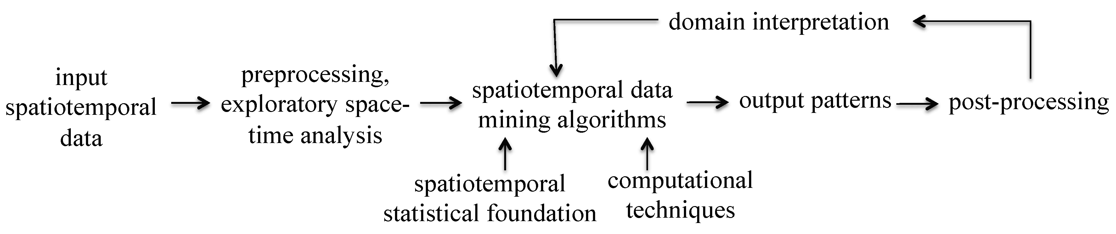
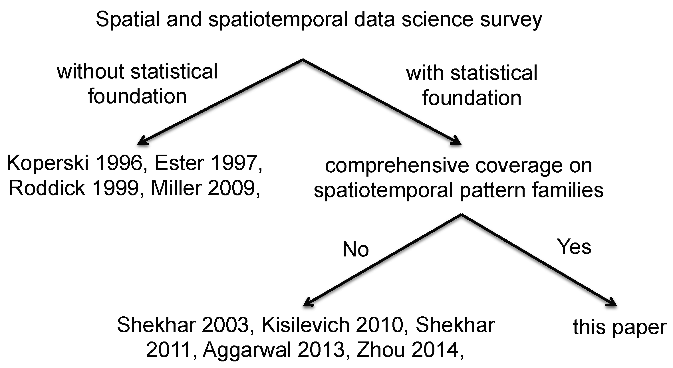
:1. Introduction


2. Input: Spatial and Spatiotemporal Data
2.1. Types of Spatial and Spatiotemporal Data

| Spatial Data | Temporal Snapshots (Time Series) | Temporal Change (Delta/Derivative) | Events/Processes | |
|---|---|---|---|---|
| object model | point(s) |
| displacement/motion (e.g., Brownian motion, random walk), speed/acceleration | spatial/spatiotemporal point process: Poisson, Cox, or Cluster process |
| line(s) | line trajectories | motion/extension/rotation, deformation, split/merge | line process | |
| polygon(s) | polygon trajectories | motion/expansion/rotation/ deformation, split/merge | flat process | |
| field model | regular, irregular | raster time series | change across raster snapshots | cellular automation |
| spatial network model | graph | spatiotemporal network:
| addition or removal of nodes and edges |
|
2.2. Data Attributes and Relationships
| Attributes | Categories | Relationships |
|---|---|---|
| non-spatial |
| Explicit
|
| spatial |
| Often implicit
|
| Spatial Data | Temporal Snapshots (Time Series) | Change (Delta/Derivative) | Event/Process | |
|---|---|---|---|---|
| object model | point(s), line(s), polygon(s) |
|
|
|
| field model | regular irregular |
| local, focal, zonal change across snapshots [29] | cellular automation [55] |
| spatial network | graph |
| change in centrality, connectivity | spatiotemporal coupling of network events |
3. Statistical Foundations
3.1. Spatial Statistics for Different Types of Spatial Data
| Spatial Model | Spatial Statistics | Spatiotemporal Statistics | |
|---|---|---|---|
| object model | point(s) | Geostatistics (point reference data)
| Statistics for spatial time series
|
Spatial Point Processes
| Spatiotemporal Point Processes
| ||
| line(s) | line process | ||
| polygon(s) | flat process | ||
| field model | regular, irregular | Lattice Statistics (areal data model)
| Statistics for raster time series
|
| spatial network | graph | Spatial Network Statistics
| |
3.2. Spatiotemporal Statistics
4. Output Pattern Families
4.1. Spatiotemporal Outlier
4.1.1. What are Spatiotemporal Outliers?
4.1.2. Application Domains
4.1.3. Statistical Foundation
4.1.4. Common Approaches

4.2. Spatiotemporal Couplings and Tele-Couplings
4.2.1. What are Spatiotemporal Couplings and Tele-Couplings?
4.2.2. Application Domains
4.2.3. Statistical Foundation
4.2.4. Common Approaches
4.3. Spatiotemporal Prediction
4.3.1. What is Spatiotemporal Prediction?
4.3.2. Application Domains
4.3.3. Statistical Foundation
4.3.4. Common Approaches
4.4. Spatiotemporal Partitioning and Summarization
4.4.1. What is Spatiotemporal Partitioning and Summarization?
4.4.2. Application Domains
4.4.3. Statistical Foundation
4.4.4. Common Approaches
| Data Types | Partition Definition | Summarization |
|---|---|---|
| classical data | partition of rows of records | aggregate statistics: sum, count, mean, etc. |
| spatial data | partition of Euclidean space | representatives: centroids, medoids, etc. |
| partition of spatial network | representatives: K main routes, etc. | |
| spatio-temporal data | partition of trajectories on a spatial or spatio-temprol network | representatives: K primary corridors, etc. |
4.5. Spatiotemporal Hotspots
4.5.1. What are Spatiotemporal Hotspots?
4.5.2. Application Domains
4.5.3. Statistical Foundation
4.5.4. Common Approaches
4.6. Spatiotemporal Change
4.6.1. What are Spatiotemporal Changes and Change Footprints
4.6.2. Common Approaches
5. Spatial and Spatiotemporal Analysis Tools
6. Research Trend and Future Research Needs
7. Summary
Acknowledgments
Author Contributions
Conflicts of Interest
References
- Stolorz, P.; Nakamura, H.; Mesrobian, E.; Muntz, R.; Shek, E.; Santos, J.; Yi, J.; Ng, K.; Chien, S.; Mechoso, R.; et al. Fast Spatio-Temporal Data Mining of Large Geophysical Datasets; AAAI Press: Palo Alto, CA, USA, 1995. [Google Scholar]
- Guting, R. An introduction to spatial database systems. VLDB J. 1994, 3, 357–399. [Google Scholar] [CrossRef]
- Shekhar, S.; Chawla, S. Spatial Databases: A Tour; Prentice Hall: Upper Saddle River, NJ, USA, 2003. [Google Scholar]
- Shekhar, S.; Chawla, S.; Ravada, S.; Fetterer, A.; Liu, X.; Lu, C.T. Spatial databases—Accomplishments and research needs. Trans. Knowl. Data Eng. 1999, 11, 45–55. [Google Scholar] [CrossRef]
- Worboys, M. GIS: A Computing Perspective; Taylor and Francis: London, UK, 1995. [Google Scholar]
- Krugman, P. Development, Geography, and Economic Theory; MIT Press: Cambridge, MA, USA, 1995. [Google Scholar]
- Albert, P.; McShane, L. A generalized estimating equations approach for spatially correlated binary data: Applications to the analysis of neuroimaging data. Biometrics 1995, 51, 627–638. [Google Scholar] [CrossRef] [PubMed]
- Shekhar, S.; Yang, T.; Hancock, P. An intelligent vehicle highway information management system. Comput.—Aided Civil Infrastruct. Eng. 1993, 8, 175–198. [Google Scholar] [CrossRef]
- Eck, J.E.; Chainey, S.; Cameron, J.G.; Leitner, M.; Wilson, R.E. Mapping Crime: Understanding Hot Spots. Available online: http://www.ncjrs.gov/pdffiles1/nij/209393.pdf (accessed on 10 May 2015).
- Issaks, E.H.; Svivastava, RM. Applied Geostatistics; Oxford University Press: Oxford, UK, 1989. [Google Scholar]
- Haining, R.J. Spatial Data Analysis in the Social and Environmental Sciences; Cambridge University Press: Cambridge, UK, 1989. [Google Scholar]
- Roddick, J.F.; Spiliopoulou, M. A bibliography of temporal, spatial and spatio-temporal data mining research. SIGKDD Explor. 1999, 1, 34–38. [Google Scholar] [CrossRef]
- Scally, R. GIS for Environmental Management; ESRI Press: Redlands, CA, USA, 2006. [Google Scholar]
- Leipnik, M.R.; Albert, D.P. GIS in Law Enforcement: Implementation Issues and Case Studies; CRC Press: Sacramento, CA, USA, 2002. [Google Scholar]
- Lang, L. Transportation GIS; ESRI Press: Redlands, CA, USA, 1999. [Google Scholar]
- Elliott, P.; Wakefield, J.; Best, N.; Briggs, D. Spatial Epidemiology: Methods and Applications; Oxford University Press: Oxford, UK, 2000. [Google Scholar]
- Hohn, M.; A.E. Liebhold, L.G. A Geostatistical model for forecasting the spatial dynamics of defoliation caused by the Gypsy Moth, Lymantria dispar (Lepidoptera:Lymantriidae). Environ. Entomol. 1993, 22, 1066–1075. [Google Scholar] [CrossRef]
- Yasui, Y.; Lele, S. A regression method for spatial disease rates: An estimating function approach. J. Am. Stat. Assoc. 1997, 94, 21–32. [Google Scholar] [CrossRef]
- Ruß, G.; Brenning, A. Data mining in precision agriculture: Management of spatial information. In Computational Intelligence for Knowledge-Based Systems Design; Springer: Berlin, Germany, 2010; pp. 350–359. [Google Scholar]
- Gubbi, J.; Buyya, R.; Marusic, S.; Palaniswami, M. Internet of Things (IoT): A vision, architectural elements, and future directions. Future Gener. Comput. Syst. 2013, 29, 1645–1660. [Google Scholar] [CrossRef]
- Marcus, G.; Davis, E. Eight (no, nine!) problems with big data. N. Y. Times 2014, 6, 2014. [Google Scholar]
- Caldwell, P.M.; Bretherton, C.S.; Zelinka, M.D.; Klein, S.A.; Santer, B.D.; Sanderson, B.M. Statistical significance of climate sensitivity predictors obtained by data mining. Geophys. Res. Lett. 2014, 41, 1803–1808. [Google Scholar] [CrossRef]
- Shekhar, S.; Zhang, P.; Huang, Y.; Vatsavai, R.R. Trends in spatial data mining. In Data Mining: Next Generation Challenges and Future Directions; AAAI Press: Palo Alto, CA, USA, 2003; pp. 357–380. [Google Scholar]
- Koperski, K.; Adhikary, J.; Han, J. Spatial data mining: Progress and challenges survey paper. In Proceedings of the ACM SIGMOD Workshop on Research Issues on Data Mining and Knowledge Discovery, Montreal, QC, Canada, 4–6 June 1996.
- Ester, M.; Kriegel, H.P.; Sander, J. Spatial Data Mining: A Database Approach. In Advances in Spatial Databases, Proceedings of the 5th International Symposium (SSD ’97), Berlin, Germany, 15–18 July 1997; Springer: Berlin, Germany, 1997; pp. 47–66. [Google Scholar]
- Miller, H.J.; Han, J. Geographic Data Mining and Knowledge Discovery; CRC Press: Sacramento, CA, USA, 2009. [Google Scholar]
- Kisilevich, S.; Mansmann, F.; Nanni, M.; Rinzivillo, S. Spatio-Temporal Clustering; Springer: Berlin, Germany, 2010. [Google Scholar]
- Aggarwal, C.C. Outlier Analysis; Springer: Berlin, Germany, 2013. [Google Scholar]
- Zhou, X.; Shekhar, S.; Ali, R.Y. Spatiotemporal change footprint pattern discovery: An inter-disciplinary survey. Wiley Interdiscip. Rev. Data Min. Knowl. Discov. 2014, 4, 1–23. [Google Scholar] [CrossRef]
- Cheng, T.; Haworth, J.; Anbaroglu, B.; Tanaksaranond, G.; Wang, J. Spatiotemporal data mining. In Handbook of Regional Science; Springer: Heidelberg, Germany, 2014; pp. 1173–1193. [Google Scholar]
- Shekhar, S.; Evans, M.R.; Kang, J.M.; Mohan, P. Identifying patterns in spatial information: A survey of methods. Wiley Interdiscip. Rev.: Data Min. Knowl. Discov. 2011, 1, 193–214. [Google Scholar] [CrossRef]
- Worboys, M.; Duckham, M. GIS: A Computing Perspective, 2nd ed.; CRC Press: Sacramento, CA, USA, 2004. [Google Scholar]
- Li, Z.; Chen, J.; Baltsavias, E. Advances in Photogrammetry, Remote Sensing and Spatial Information Sciences: 2008 ISPRS Congress Book; CRC Press: Sacramento, CA, USA, 2008. [Google Scholar]
- Yuan, M. Temporal GIS and spatio-temporal modeling. In Proceedings of the Third International Conference Workshop on Integrating GIS and Environment Modeling, Santa Fe, NM, USA, 21–26 January 1996.
- Allen, J.F. Towards a general theory of action and time. Artif. Intell. 1984, 23, 123–154. [Google Scholar] [CrossRef]
- George, B.; Kim, S.; Shekhar, S. Spatio-temporal Network Databases and Routing Algorithms: A Summary of Results. In Proceedings of the 10th International Symposium on Spatial and Temporal Databases (SSTD’07), Boston, MA, USA, 16–18 July 2007.
- George, B.; Shekhar, S. Time Aggregated Graphs: A model for spatio-temporal network. In Proceedings of the Workshops (CoMoGIS) at the 25th International Conference on Conceptual Modeling (ER2006), Tucson, AZ, USA, 6–9 November 2006.
- Gelfand, A.E.; Diggle, P.; Guttorp, P.; Fuentes, M. Handbook of Spatial Statistics; CRC Press: Sacramento, CA, USA, 2010. [Google Scholar]
- Campelo, C.E.; Bennett, B. Representing and Reasoning about Changing Spatial Extensions of Geographic Features; Springer: Berlin, Germany, 2013. [Google Scholar]
- Tan, P.N.; Steinbach, M.; Kumar, V. Introduction to Data Mining; Pearson Addison Wesley: Boston, MA, USA, 2006. [Google Scholar]
- Bolstad, P. GIS Fundamentals: A First Text on GIS; Eider Press: Saint Paul, MN, USA, 2002. [Google Scholar]
- Ganguly, A.R.; Steinhaeuser, K. Data Mining for Climate Change and Impacts. In Proceedings of the 2008 IEEE International Conference on Data Mining Workshops (ICDMW ’08), Pisa, Italy, 15–19 December 2008; pp. 385–394.
- Erwig, M.; Schneider, M.; Hagen, F. Spatio-temporal predicates. IEEE Trans. Knowl. Data Eng. 2002, 14, 881–901. [Google Scholar] [CrossRef]
- Chen, J.; Wang, R.; Liu, L.; Song, J. Clustering of trajectories based on Hausdorff distance. In Proceedings of the 2011 IEEE International Conference on Electronics, Communications and Control (ICECC), Ningbo, China, 9–11 September 2011; pp. 1940–1944.
- Zhang, Z.; Huang, K.; Tan, T. Comparison of similarity measures for trajectory clustering in outdoor surveillance scenes. In Proceedings of the 18th IEEE International Conference on Pattern Recognition (ICPR 2006), Hong Kong, China, 20–24 August 2006; Volume 3, pp. 1135–1138.
- Zhang, P.; Huang, Y.; Shekhar, S.; Kumar, V. Correlation analysis of spatial time series datasets: A filter-and-refine approach. In Advances in Knowledge Discovery and Data Mining; Springer: Berlin, Germany, 2003; pp. 532–544. [Google Scholar]
- Kawale, J.; Chatterjee, S.; Ormsby, D.; Steinhaeuser, K.; Liess, S.; Kumar, V. Testing the significance of spatio-temporal teleconnection patterns. In Proceedings of the 18th ACM SIGKDD International Conference on Knowledge Discovery and Data Mining, Beijing, China, 12–16 August 2012; pp. 642–650.
- Celik, M.; Shekhar, S.; Rogers, J.P.; Shine, J.A.; Yoo, J.S. Mixed-drove spatio-temporal co-occurence pattern mining: A summary of results. In Proceedings of the Sixth International Conference on Data Mining, Washington, DC, USA, 18–22 December 2006.
- Pillai, K.G.; Angryk, R.A.; Aydin, B. A Filter-and-Refine Approach to Mine Spatiotemporal Co-Occurrences; SIGSPATIAL/GIS: Orlando, USA, 2013; pp. 104–113. [Google Scholar]
- Mohan, P.; Shekhar, S.; Shine, J.A.; Rogers, J.P. Cascading spatio-temporal pattern discovery. IEEE Trans. Knowl. Data Eng. 2012, 24, 1977–1992. [Google Scholar] [CrossRef]
- Mohan, P.; Shekhar, S.; Shine, J.A.; Rogers, J.P. Cascading Spatio-Temporal Pattern Discovery: A Summary of Results; SDM: Columbus, USA, 2010. [Google Scholar]
- Huang, Y.; Zhang, L.; Zhang, P. A framework for mining sequential patterns from spatio-temporal event data sets. IEEE Trans. Knowl. Data Eng. 2008, 20, 433–448. [Google Scholar] [CrossRef]
- Huang, Y.; Zhang, L.; Zhang, P. Finding Sequential Patterns from a Massive Number of Spatio-Temporal Events; SDM: Bethesda, USA, 2006. [Google Scholar]
- Mennis, J.; Viger, R.; Tomlin, C.D. Cubic map algebra functions for spatio-temporal analysis. Cartogr. Geogr. Inf. Sci. 2005, 32, 17–32. [Google Scholar] [CrossRef]
- Brown, D.G.; Riolo, R.; Robinson, D.T.; North, M.; Rand, W. Spatial process and data models: Toward integration of agent-based models and GIS. J. Geogr. Syst. 2005, 7, 25–47. [Google Scholar] [CrossRef]
- Habiba, H.; Tantipathananandh, C.; Berger-Wolf, T. Betweenness Centrality Measure in Dynamic Networks; Department of Computer Science, University of Illinois at Chicago: Chicago, IL, USA, 2007. [Google Scholar]
- Kang, J.M.; Shekhar, S.; Wennen, C.; Novak, P. Discovering flow anomalies: A SWEET approach. In Proceedings of the 8th IEEE International Conference on Data Mining (ICDM ’08), Pisa, Italy, 15–19 December 2008.
- Kang, J.M.; Shekhar, S.; Henjum, M.; Novak, P.; Arnold, W. Discovering teleconnected flow anomalies: A relationship analysis of spatio-temporal Dynamic (RAD) neighborhoods. In Proceedings of 11th International Symposium (SSTD 2009), Aalborg, Denmark, 8–10 July 2009.
- Ahuja, R.K.; Magnanti, T.L.; Orlin, J.B. Network Flows: Theory, Algorithms, and Applications; Prentice Hall: Upper Saddle River, NJ, USA, 1988. [Google Scholar]
- Quinlan, J. C4.5: Programs for Machine Learning; Morgan Kaufmann Publishers: Burlington, MA, USA, 1993. [Google Scholar]
- Varnett, V.; Lewis, T. Outliers in Statistical Data; John Wiley: Hoboken, NJ, USA, 1994. [Google Scholar]
- Agarwal, R.; Imielinski, T.; Swami, A. Mining association rules between sets of items in large databases. In Proceedings of the ACM SIGMOD Conference on Management of Data, Washington, DC, USA, 26–28 May 1993.
- Agrawal, R.; Srikant, R. Fast algorithms for mining association rules. In Proceedings of the 20th International Conference on Very Large Data Bases, Santiago de Chile, Chile, 12–15 September 1994.
- Jain, A.; Dubes, R. Algorithms for Clustering Data; Prentice Hall: Upper Saddle River, NJ, USA, 1988. [Google Scholar]
- Tobler, W. Cellular Geography, Philosophy in Geography; Reidel: Dordrecht, Netherlands, 1979. [Google Scholar]
- Banerjee, S.; Carlin, B.; Gelfand, A. Hierarchical Modeling and Analysis for Spatial Data; Chapman & Hall: London, UK, 2004. [Google Scholar]
- Schabenberger, O.; Gotway, C. Statistical Methods for Spatial Data Analysis; Chapman and Hall: London, UK, 2005. [Google Scholar]
- Cressie, N.A.C. Statistics for Spatial Data; Wiley: New York, NY, USA, 1993. [Google Scholar]
- Cressie, N. Statistics for Spatial Data (Revised Edition); Wiley: New York, NY, USA, 1993. [Google Scholar]
- Gething, P.W.; Atkinson, P.M.; Noor, A.; Gikandi, P.; Hay, S.I.; Nixon, M.S. A local space-time kriging approach applied to a national outpatient malaria data set. Comput. Geosci. 2007, 33, 1337–1350. [Google Scholar] [CrossRef] [PubMed] [Green Version]
- Warrender, C.E.; Augusteijn, M.F. Fusion of image classifications using Bayesian techniques with Markov rand fields. Int. J. Remote Sens. 1999, 20, 1987–2002. [Google Scholar] [CrossRef]
- Anselin, L. Local indicators of spatial association-LISA. Geogr. Anal. 1995, 27, 93–155. [Google Scholar] [CrossRef]
- Openshaw, S. The Modifiable Areal Unit Problem; OCLC: Dublin, OH, USA, 1983. [Google Scholar]
- Ripley, B.D. Modelling spatial patterns. J. R. Stat. Soc. Ser. B (Methodol.) 1977, 39, 172–212. [Google Scholar]
- Marcon, E.; Puech, F. Generalizing Ripley’s K Function to Inhomogeneous Populations; Mimeo: New York, NY, USA, 2003. [Google Scholar]
- Kulldorff, M. A spatial scan statistic. Commun. Stat.-Theory Methods 1997, 26, 1481–1496. [Google Scholar] [CrossRef]
- Chiu, S.N.; Stoyan, D.; Kendall, W.S.; Mecke, J. Stochastic Geometry and Its Applications; John Wiley & Sons: New York, NY, USA, 2013. [Google Scholar]
- Guyon, X. Random Fields on a Network: Modeling, Statistics, and Applications; Springer: Berlin, Germany, 1995. [Google Scholar]
- Okabe, A.; Yomono, H.; Kitamura, M. Statistical analysis of the distribution of points on a network. Geogr. Anal. 1995, 27, 152–175. [Google Scholar] [CrossRef]
- Okabe, A.; Sugihara, K. Spatial Analysis along Networks: Statistical and Computational Methods; John Wiley & Sons: New York, NY, USA, 2012. [Google Scholar]
- Okabe, A.; Okunuki, K.; Shiode, S. The SANET Toolbox: New methods for network spatial analysis. Trans. GIS 2006, 10, 535–550. [Google Scholar] [CrossRef]
- Cressie, N.; Wikle, C.K. Statistics for Spatio-Temporal Data; John Wiley & Sons: New York, NY, USA, 2011. [Google Scholar]
- Shumway, R.H.; Stoffer, D.S. Time Series Analysis and Its Applications: With R Examples; Springer: Berlin, Germany, 2010. [Google Scholar]
- Kyriakidis, P.C.; Journel, A.G. Geostatistical space-time models: A review. Math. Geol. 1999, 31, 651–684. [Google Scholar] [CrossRef]
- Cressie, A.C.N. Statistics for Spatial Data; Wiley-Interscience: Hoboken, NJ, USA, 1993. [Google Scholar]
- Barnett, V.; Lewis, T. Outliers in Statistical Data, 3rd ed.; John Wiley: Hoboken, NJ, USA, 1994. [Google Scholar]
- Hawkins, D. Identification of Outliers; Chapman and Hall: London, UK, 1980. [Google Scholar]
- Chandola, V.; Banerjee, A.; Kumar, V. Anomaly Detection: A Survey. ACM Comput. Surv. 2009, 41, 1–58. [Google Scholar] [CrossRef]
- Shekhar, S.; Lu, C.; Zhang, P. Graph-based outlier detection: Algorithms and applications (a summary of results). In Proceedings of the Seventh ACM SIGKDD International Conference on Knowledge Discovery and Data Mining, San Francisco, CA, USA, 26–29 August 2001.
- Wu, W.; Cheng, X.; Ding, M.; Xing, K.; Liu, F.; Deng, P. Localized outlying and boundary data detection in sensor networks. IEEE Trans. Knowl. Data Eng. 2007, 19, 1145–1157. [Google Scholar] [CrossRef]
- Sun, P.; Chawla, S. On local spatial outliers. In Proceedings of the Fourth IEEE International Conference on Data Mining (ICDM ’04), Brighton, UK, 1–4 November 2004; pp. 209–216.
- Pei, Y.; Zaıane, O.R.; Gao, Y. An efficient reference-based approach to outlier detection in large Datasets. In Proceedings of the Sixth International Conference on Data Mining (ICDM ’06), Hong Kong, China, 18–22 December 2006; pp. 478–487.
- Shekhar, S.; Lu, C.; Zhang, P. A unified approach to detecting spatial outliers. GeoInformatica 2003, 7, 139–166. [Google Scholar] [CrossRef]
- Shekhar, S.; Lu, C.; Zhang, P. Detecting graph-based spatial outliers: Algorithms and applications. In Proceedings of the 7th ACM SIGKDD International Conference on Knowledge Discovery and Data Mining, San Francisco, CA, USA, 26–29 August 2001.
- Haslett, J.; Bradley, R.; Craig, P.; Unwin, A.; Wills, G. Dynamic graphics for exploring spatial data with application to locating global and local anomalies. Am. Stat. 1991, 45, 234–242. [Google Scholar]
- Luc, A. Local indicators of spatial association: LISA. Geogr. Anal. 1995, 27, 93–115. [Google Scholar]
- Luc, A. Exploratory spatial data analysis and geographic information systems. In New Tools for Spatial Analysis; Wiley: Hoboken, NJ, USA, 1994; pp. 45–54. [Google Scholar]
- Chen, F.; Lu, C.T.; Boedihardjo, A.P. GLS-SOD: A Generalized Local Statistical Approach for Spatial Outlier Detection; KDD: Washington, DC, USA, 2010. [Google Scholar]
- Lu, C.T.; Chen, D.; Kou, Y. Algorithms for spatial outlier detection. In Proceedings of the 3rd International Conference on Data Mining (ICDM ’03), Melbourne, FL, USA, 19–22 November 2003; pp. 597–600.
- Chen, D.; Lu, C.T.; Kou, Y.; Chen, F. On detecting spatial outliers. GeoInformatica 2008, 12, 455–475. [Google Scholar] [CrossRef]
- McGuire, M.P.; Janeja, V.P.; Gangopadhyay, A. Mining trajectories of moving dynamic spatio-temporal regions in sensor datasets. Data Min. Knowl. Discov. 2014, 28, 961–1003. [Google Scholar] [CrossRef]
- Lu, C.T.; Chen, D.; Kou, Y. Detecting spatial outliers with multiple attributes. In Proceedings of the 15th IEEE International Conference on Tools with Artificial Intelligence, Washington, DC, USA, 3–5 November 2003.
- Kou, Y.; Lu, C.T.; Chen, D. Spatial Weighted Outlier Detection; SDM: Bethesda, USA, 2006. [Google Scholar]
- Liu, X.; Chen, F.; Lu, C.T. On detecting spatial categorical outliers. GeoInformatica 2014, 18, 501–536. [Google Scholar] [CrossRef]
- Schubert, E.; Zimek, A.; Kriegel, H.P. Local outlier detection reconsidered: A generalized view on locality with applications to spatial, video, and network outlier detection. Data Min. Knowl. Discov. 2014, 28, 190–237. [Google Scholar] [CrossRef]
- Wu, M.; Song, X.; Jermaine, C.; Ranka, S.; Gums, J. A LRT Framework for Fast Spatial Anomaly Detection; KDD: Paris, France, 2009. [Google Scholar]
- Wu, M.; Jermaine, C.; Ranka, S.; Song, X.; Gums, J. A model-agnostic framework for fast spatial anomaly detection. TKDD 2010, 4. [Google Scholar] [CrossRef]
- Franke, C.; Gertz, M. Detection and exploration of outlier regions in sensor data streams. In Proceedings of the IEEE International Conference on Data Mining Workshops (ICDMW ’08), Pisa, Italy, 15–19 December 2008; pp. 375–384.
- Elfeky, M.G.; Aref, W.G.; Elmagarmid, A.K. STAGGER: Periodicity mining of data streams using expanding sliding windows. In Proceedings of the Sixth International Conference on Data Mining (ICDM ’06), Hong Kong, China, 18–22 December 2006; pp. 188–199.
- Liu, C.; Xiong, H.; Ge, Y.; Geng, W.; Perkins, M. A stochastic model for context-aware anomaly detection in indoor location traces. In Proceedings of the 12th International Conference on Data Mining (ICDM ’12), Brussels, Belgium, 10–13 December 2012; pp. 449–458.
- Bu, Y.; Chen, L.; Fu, A.W.C.; Liu, D. Efficient anomaly monitoring over moving object trajectory streams. In Proceedings of the 15th ACM SIGKDD International Conference on Knowledge Discovery and Data Mining, Paris, France, 28 June–1 July 2009; pp. 159–168.
- Li, X.; Han, J.; Kim, S. Motion-alert: Automatic anomaly detection in massive moving objects. In Intelligence and Security Informatics; Springer: Berlin, Germany, 2006; pp. 166–177. [Google Scholar]
- Ge, Y.; Xiong, H.; Liu, C.; Zhou, Z.H. A taxi driving fraud detection system. In Proceedings of the 2011 IEEE International Conference on Data Mining (ICDM), Vancouver, BC, Canada, 11–14 December 2011; pp. 181–190.
- Zhang, D.; Li, N.; Zhou, Z.H.; Chen, C.; Sun, L.; Li, S. iBAT: Detecting anomalous taxi trajectories from GPS traces. In Proceedings of the 13th International Conference on Ubiquitous Computing, Beijing, China, 17–21 September 2011; pp. 99–108.
- Chen, C.; Zhang, D.; Castro, P.S.; Li, N.; Sun, L.; Li, S. Real-time detection of anomalous taxi trajectories from GPS traces. In Mobile and Ubiquitous Systems: Computing, Networking, and Services; Springer: Berlin, Germany, 2012; pp. 63–74. [Google Scholar]
- Scott, M.S.; Dedel, K. Assaults in and Around Bars, 2nd ed.; Office of Community Oriented Policing Services: Washington, DC, USA, 2006. [Google Scholar]
- Lynch, H.J.; Moorcroft, P.R. A spatiotemporal Ripley’s K-function to analyze interactions between spruce budworm and fire in British Columbia, Canada. Can. J. For. Res. 2008, 38, 3112–3119. [Google Scholar] [CrossRef]
- Guting, R.; Schneider, M. Moving Object Databases; Morgan Kaufmann: Burlington, MA, USA, 2005. [Google Scholar]
- Koubarakis, M.; Sellis, T.; Frank, A.; Grumbach, S.; Guting, R.; Jensen, C.; Lorentzos, N.; Schek, H.J.; Scholl, M. Spatio-Temporal Databases: The Chorochronos Approach, LNCS 2520; Springer: Berlin, Germany, 2003; Volume 9. [Google Scholar]
- Celik, M.; Shekhar, S.; Rogers, J.P.; Shine, J.A. Mixed-drove spatiotemporal co-occurrence pattern mining. IEEE Trans. Knowl. Data Eng. 2008, 20, 1322–1335. [Google Scholar] [CrossRef]
- Cao, H.; Mamoulis, N.; Cheung, D.W. Mining frequent spatio-temporal sequential patterns. In Proceedings of the 5th International Conference on Data Mining (ICDM ’05), New Orleans, LA, USA, 26–30 November 2005; pp. 82–89.
- Verhein, F. Mining Complex Spatio-Temporal Sequence Patterns; SDM: Sparks, USA, 2009. [Google Scholar]
- Li, Y.; Bailey, J.; Kulik, L.; Pei, J. Mining probabilistic frequent spatio-temporal sequential patterns with gap constraints from uncertain databases. In Proceedings of the 13th International Conference on Data Mining (ICDM ’13), Dallas, TX, USA, 7–10 December 2013; pp. 448–457.
- Strategic Plan for the Climate change Science Program. 2003. Available online: http://www.climatescience.gov/Library/stratplan2003/final/ccspstratplan2003-chap9.htm (accessed on 15 May 2015).
- Frelich, L.E.; Reich, P.B. Will environmental changes reinforce the impact of global warming on the prairie-forest border of central north america? Front. Ecol. Environ. 2009, 8, 371–378. [Google Scholar] [CrossRef]
- Morens, D.M.; Folkers, G.K.; Fauci, A.S. The challenge of emerging and re-emerging infectious diseases. Nature 2004, 430, 242–249. [Google Scholar] [CrossRef] [PubMed]
- Zhang, P.; Huang, Y.; Shekhar, S.; Kumar, V. Exploiting spatial autocorrelation to efficiently process correlation-based similarity queries. In Proceedings of the 8th International Symposium on Advances in Spatial and Temporal Databases (SSTD 2003), Santorini Island, Greece, 24–27 July 2003; pp. 449–468.
- De Almeida, C.M.; Souza, I.M.; Alves, C.D.; Pinho, C.M.D.; Pereira, M.N.; Feitosa, R.Q. Multilevel object-oriented classification of quickbird images for urban population estimates. In Proceedings of the 15th ACM International Symposium on Geographic Information Systems, Seattle, USA, 2007; p. 12.
- Little, B.; Schucking, M.; Gartrell, B.; Chen, B.; Ross, K.; McKellip, R. High granularity remote sensing and crop production over space and time: NDVI over the growing season and prediction of cotton yields at the farm field level in Texas. In Proceedings of the IEEE International Conference on Data Mining Workshops (ICDMW ’08), Pisa, Italy, 15–19 December 2008; pp. 426–435.
- Friedl, M.A.; Brodley, C.E. Decision tree classification of land cover from remotely sensed data. Remote Sens. Environ. 1997, 61, 399–409. [Google Scholar] [CrossRef]
- Subbian, K.; Banerjee, A. Climate Multi-Model Regression Using Spatial Smoothing; SDM: Austin, USA, 2013. [Google Scholar]
- Pace, R.K.; Barry, R.; Clapp, J.M.; Rodriquez, M. Spatiotemporal autoregressive models of neighborhood effects. J. Real Estate Financ. Econ. 1998, 17, 15–33. [Google Scholar] [CrossRef]
- Elhorst, J.P. Specification and estimation of spatial panel data models. Int. Reg. Sci. Rev. 2003, 26, 244–268. [Google Scholar] [CrossRef]
- Anselin, L. Spatial Econometrics: Methods and Models; Kluwer: Dordrecht, Netherlands, 1988. [Google Scholar]
- Levine, N. CrimeStat 3.0: A Spatial Statistics Program for the Analysis of Crime Incident Locations; Ned Levine & Associatiates: Houston, TX, USA, 2004. [Google Scholar]
- Han, J.; Kamber, M.; Tung, A.K.H. Spatial Clustering Methods in Data Mining: A Survey; Taylor and Francis: London, UK, 2001. [Google Scholar]
- Agrawal, R.; Gehrke, J.; Gunopulos, D.; Raghavan, P. Automatic Subspace Clustering of High Dimensional Data for Data Mining Applications; ACM: New York, NY, USA, 1998. [Google Scholar]
- Ng, R.T.; Han, J. CLARANS: A method for clustering objects for spatial data mining. IEEE Trans. Knowl. Data Eng. 2002, 14, 1003–1016. [Google Scholar] [CrossRef]
- Birant, D.; Kut, A. ST-DBSCAN: An algorithm for clustering spatial-temporal data. Data Knowl. Eng. 2007, 60, 208–221. [Google Scholar] [CrossRef]
- Ester, M.; Kriegel, H.P.; Sander, J.; Xu, X. A density-based algorithm for discovering clusters in large spatial databases with noise. Kdd 1996, 96, 226–231. [Google Scholar]
- Ankerst, M.; Breunig, M.M.; Kriegel, H.P.; Sander, J. OPTICS: Ordering points to identify the clustering structure. In ACM Sigmod Record; ACM: New York, NY, USA, 1999; Volume 28, pp. 49–60. [Google Scholar]
- Wang, M.; Wang, A.; Li, A. Mining spatial-temporal clusters from geo-databases. In Advanced Data Mining and Applications; Springer: Berlin, Germany, 2006; pp. 263–270. [Google Scholar]
- Zhang, T.; Ramakrishnan, R.; Livny, M. BIRCH: An Efficient Data Clustering Method for Very Large Databases. In ACM SIGMOD Record, Proceedings of the 1996 ACM SIGMOD International Conference on Management of Data, Montreal, QC, Canada, 4–6 June 1996; Jagadish, H.V., Mumick, I.S., Eds.; ACM Press: New York, NY, USA, 1996; pp. 103–114. [Google Scholar]
- Karypis, G.; Han, E.H.; Kumar, V. Chameleon: Hierarchical clustering using dynamic modeling. IEEE Comput. 1999, 32, 68–75. [Google Scholar] [CrossRef]
- Lee, J.G.; Han, J.; Whang, K.Y. Trajectory clustering: A partition-and-group framework. In Proceedings of the 2007 ACM SIGMOD International Conference on Management of Data; ACM: New York, NY, USA, 2007; pp. 593–604. [Google Scholar]
- Sander, J.; Ester, M.; Kriegel, H.P.; Xu, X. Density-based clustering in spatial databases: The algorithm gdbscan and its applications. Data Min. Knowl. Discov. 1998, 2, 169–194. [Google Scholar] [CrossRef]
- Lee, A.J.; Chen, Y.A.; Ip, W.C. Mining frequent trajectory patterns in spatial-temporal databases. Inf. Sci. 2009, 179, 2218–2231. [Google Scholar] [CrossRef]
- Chandola, V.; Kumar, V. Summarization-compressing data into an informative representation. Knowl. Inf. Syst. 2007, 12, 355–378. [Google Scholar] [CrossRef]
- Pan, B.; Demiryurek, U.; Banaei-Kashani, F.; Shahabi, C. Spatiotemporal summarization of traffic data streams. In Proceedings of the ACM SIGSPATIAL International Workshop on GeoStreaming, San Jose, CA, USA, 3–5 November 2010; pp. 4–10.
- Evans, M.R.; Oliver, D.; Shekhar, S.; Harvey, F. Summarizing trajectories into k-primary corridors: A summary of results. In Proceedings of the 20th International Conference on Advances in Geographic Information Systems, Redondo Beach, CA, USA, 6–9 November 2012; pp. 454–457.
- Evans, M.R.; Oliver, D.; Shekhar, S.; Harvey, F. Fast and Exact Network Trajectory Similarity Computation: A Case-study on Bicycle Corridor Planning. In Proceedings of the 2nd ACM SIGKDD International Workshop on Urban Computing; ACM: New York, NY, USA, 2013; pp. 9:1–9:8. [Google Scholar]
- Kulldorff, M. SaTScan User Guide for Version 9.0. Available online: www.satscan.org (accessed on 15 May 2015).
- Jain, A.; Murty, M.; Flynn, P. Data clustering: A review. ACM Comput. Surv. (CSUR) 1999, 31, 264–323. [Google Scholar] [CrossRef]
- Chang, W.; Zeng, D.; Chen, H. Prospective spatio-temporal data analysis for security informatics. In Proceedings of the 2005 IEEE Intelligent Transportation Systems, Vienna, Austria, 13–15 September 2005; pp. 1120–1124.
- Tango, T.; Takahashi, K.; Kohriyama, K. A space-time scan statistic for detecting emerging outbreaks. Biometrics 2011, 67, 106–115. [Google Scholar] [CrossRef] [PubMed]
- Neill, D.; Moore, A.; Sabhnani, M.; Daniel, K. Detection of emerging space-time clusters. In Proceedings of the 11th ACM SIGKDD International Conference on Knowledge Discovery in Data Mining, Chicago, IL, USA, 21–24 August 2005; pp. 218–227.
- Chandola, V.; Hui, D.; Gu, L.; Bhaduri, B.; Vatsavai, R. Using time series segmentation for deriving negetation phenology indices from MODIS NDVI data. In Proceedings of the 2010 IEEE International Conference on Data Mining Workshops (ICDMW), Sydney, NSW, Australia, 13 December 2010.
- Worboys, M.; Duckham, M. GIS: A Computing Perspective; CRC Press: Sacramento, CA, USA, 2004. [Google Scholar]
- Bujor, F.; Trouvé, E.; Valet, L.; Nicolas, J.M.; Rudant, J.P. Application of log-cumulants to the detection of spatiotemporal discontinuities in multitemporal SAR images. IEEE Trans. Geosci. Remote Sens. 2004, 42, 2073–2084. [Google Scholar] [CrossRef]
- Kosugi, Y.; Sakamoto, M.; Fukunishi, M.; Lu, W.; Doihara, T.; Kakumoto, S. Urban change detection related to earthquakes using an adaptive nonlinear mapping of high-resolution images. IEEE Geosci. Remote Sens. Lett. 2004, 1, 152–156. [Google Scholar] [CrossRef]
- Di Martino, G.; Iodice, A.; Riccio, D.; Ruello, G. A novel approach for disaster monitoring: Fractal models and tools. IEEE Trans. Geosci. Remote Sens. 2007, 45, 1559–1570. [Google Scholar] [CrossRef]
- Radke, R.; Andra, S.; Al-Kofahi, O.; Roysam, B. Image change detection algorithms: A systematic survey. IEEE Trans. Image Process. 2005, 14, 294–307. [Google Scholar] [CrossRef] [PubMed]
- Thoma, R.; Bierling, M. Motion compensating interpolation considering covered and uncovered background. Signal Process.: Image Commun. 1989, 1, 191–212. [Google Scholar] [CrossRef]
- Aach, T.; Kaup, A. Bayesian algorithms for adaptive change detection in image sequences using Markov random fields. Signal Process.: Image Commun. 1995, 7, 147–160. [Google Scholar] [CrossRef]
- Chen, G.; Hay, G.J.; Carvalho, L.M.; Wulder, M.A. Object-based change detection. Int. J. Remote Sens. 2012, 33, 4434–4457. [Google Scholar] [CrossRef]
- Desclee, B.; Bogaert, P.; Defourny, P. Forest change detection by statistical object-based method. Remote Sens. Environ. 2006, 102, 1–11. [Google Scholar] [CrossRef]
- Im, J.; Jensen, J.; Tullis, J. Object-based change detection using correlation image analysis and image segmentation. Int. J. Remote Sens. 2008, 29, 399–423. [Google Scholar] [CrossRef]
- Aach, T.; Kaup, A.; Mester, R. Statistical model-based change detection in moving video. Signal Process. 1993, 31, 165–180. [Google Scholar] [CrossRef]
- Rignot, E.J.; van Zyl, J.J. Change detection techniques for ERS-1 SAR data. IEEE Trans. Geosci. Remote Sens. 1993, 31, 896–906. [Google Scholar] [CrossRef]
- Im, J.; Jensen, J. A change detection model based on neighborhood correlation image analysis and decision tree classification. Remote Sens. Environ. 2005, 99, 326–340. [Google Scholar] [CrossRef]
- Yakimovsky, Y. Boundary and object detection in real world images. J. ACM (JACM) 1976, 23, 599–618. [Google Scholar] [CrossRef]
- Douglas, D.H.; Peucker, T.K. Algorithms for the reduction of the number of points required to represent a digitized line or its caricature. Cartogr. Int. J. Geogr. Inf. Geovisualization 1973, 10, 112–122. [Google Scholar] [CrossRef]
- Kulldorff, M.; Athas, W.; Feurer, E.; Miller, B.; Key, C. Evaluating cluster alarms: A space-time scan statistic and brain cancer in Los Alamos, New Mexico. Am. J. Public Health 1998, 88, 1377–1380. [Google Scholar] [CrossRef] [PubMed]
- Kulldorff, M. Prospective time periodic geographical disease surveillance using a scan statistic. J. R. Stat. Soc. Ser. A (Stat. Soc.) 2001, 164, 61–72. [Google Scholar] [CrossRef]
- Website, A. ArcGIS. Available online: http://www.arcgis.com/ (accessed on 15 May 2015).
- Website, Q. QGIS: A Free and Open Source Geographic Information System. Available online: http://www.qgis.org/ (accessed on 15 May 2015).
- Bivand, R. CRAN Task View: Analysis of Spatial Data. Available online: https://cran.r-project.org/web/views/Spatial.html (accessed 15 May 2015).
- MathWorks. Mapping Toolbox in Matlab. Available online: http://www.mathworks.com/products/mapping/ (accessed on 15 May 2015).
- SAS. Spatial Analysis in SAS. Available online: http://support.sas.com/rnd/app/stat/procedures/SpatialAnalysis.html (accessed on 15 May 2015).
- Beinat, E.; Godfrind, A.; Kothuri, R.V. Pro Oracle Spatial; Apress: New York, NY, USA, 2004. [Google Scholar]
- Chamberlin, D. Using the New DB2: IBM’s Object Relational System; Ap Professional: Waltham, USA, 1997. [Google Scholar]
- PostGIS. Available online: http://postgis.refractions.net/ (accessed on 15 May 2015).
- ESRI. Breathe Life into Big Data: ArcGIS Tools and Hadoop Analyze Large Data Stores. Available online: http://www.esri.com/esriOnews/arcnews/summer13articles/breatheOlifeOintoObigOdata! (accessed on 15 May 2015).
- ESRI. ESRI: GIS and Mapping Software. Available online: http://www.esri.com (accessed on 15 May 2015).
- Aji, A.; Wang, F.; Vo, H.; Lee, R.; Liu, Q.; Zhang, X.; Saltz, J. Hadoop GIS: A high performance spatial data warehousing system over mapreduce. Proc. VLDB Endow. 2013, 6, 1009–1020. [Google Scholar] [CrossRef]
- Eldawy, A.; Mokbel, M.F. SpatialHadoop: A MapReduce framework for spatial data. In Proceedings of the IEEE International Conference on Data Engineering (ICDE’15), Seoul, Korea, 13–17 April 2015.
- Isaak, D.J.; Peterson, E.E.; Ver Hoef, J.M.; Wenger, S.J.; Falke, J.A.; Torgersen, C.E.; Sowder, C.; Steel, E.A.; Fortin, M.J.; Jordan, C.E.; et al. Applications of spatial statistical network models to stream data. Wiley Interdiscip. Rev.: Water 2014, 1, 277–294. [Google Scholar] [CrossRef]
- Oliver, D.; Bannur, A.; Kang, J.M.; Shekhar, S.; Bousselaire, R. A k-main routes approach to spatial network activity summarization: A summary of results. In Proceedings of the 2010 IEEE International Conference on Data Mining Workshops (ICDMW), Sydney, NSW, Australia, 13 December 2010; pp. 265–272.
- Oliver, D.; Shekhar, S.; Kang, J.M.; Laubscher, R.; Carlan, V.; Bannur, A. A k-main routes approach to spatial network activity summarization. IEEE Trans. Knowl. Data Eng. 2014, 26, 1464–1478. [Google Scholar] [CrossRef]
- Gunturi, V.M.V.; Shekhar, S. Lagrangian xgraphs: A logical data-model for spatio-temporal network data: A summary. In Proceedings of the Advances in Conceptual Modeling—ER 2014 Workshops, ENMO, MoBiD, MReBA, QMMQ, SeCoGIS, WISM, and ER Demos, Atlanta, GA, USA, 27–29 October 2014; pp. 201–211.
- Gunturi, V.M.; Nunes, E.; Yang, K.; Shekhar, S. A critical-time-point approach to all-start-time lagrangian shortest paths: A summary of results. In Advances in Spatial and Temporal Databases; Pfoser, D., Tao, Y., Mouratidis, K., Nascimento, M., Mokbel, M., Shekhar, S., Huang, Y., Eds.; Springer: Berlin/Heidelberg, Germany, 2011; Volume 6849, pp. 74–91. [Google Scholar]
- Gunturi, V.; Shekhar, S.; Yang, K. A Critical-time-point Approach to All-departure-time Lagrangian Shortest Paths. IEEE Trans. Knowl. Data Eng. 2015, 27, 2591–2603. [Google Scholar] [CrossRef]
- Speed, J. IoT for V2V and the Connected Car. Available online: http://www.slideshare.net/JoeSpeed/aw-megatrends-2014-joe-speed (accessed on May 15 2015).
- Ali, R.Y.; Gunturi, V.M.; Kotz, A.; Shekhar, S.; Northrop, W. Discovering non-compliant window co-occurrence patterns: A summary of results. In Proceedings of the 14th International Symposium on Spatial and Temporal Databases, Seoul, South Korea, 26–28 August 2015.
- Avery, C. Giraph: Large-scale graph processing infrastructure on hadoop. In Proceedings of the Hadoop Summit, Santa Clara, CA, USA, 29 June 2011.
- Low, Y.; Gonzalez, J.E.; Kyrola, A.; Bickson, D.; Guestrin, C.E.; Hellerstein, J. Graphlab: A New Framework for Parallel Machine Learning. Available online: http://arxiv.org/pdf/1408.2041 (accessed on 15 May 2015).
- Malewicz, G.; Austern, M.H.; Bik, A.J.; Dehnert, J.C.; Horn, I.; Leiser, N.; Czajkowski, G. Pregel: A system for large-scale graph processing. In Proceedings of the 2010 ACM SIGMOD International Conference on Management of Data, Indianapolis, IN, USA, 6–11 June 2010; pp. 135–146.
© 2015 by the authors; licensee MDPI, Basel, Switzerland. This article is an open access article distributed under the terms and conditions of the Creative Commons Attribution license (http://creativecommons.org/licenses/by/4.0/).
Share and Cite
Shekhar, S.; Jiang, Z.; Ali, R.Y.; Eftelioglu, E.; Tang, X.; Gunturi, V.M.V.; Zhou, X. Spatiotemporal Data Mining: A Computational Perspective. ISPRS Int. J. Geo-Inf. 2015, 4, 2306-2338. https://0-doi-org.brum.beds.ac.uk/10.3390/ijgi4042306
Shekhar S, Jiang Z, Ali RY, Eftelioglu E, Tang X, Gunturi VMV, Zhou X. Spatiotemporal Data Mining: A Computational Perspective. ISPRS International Journal of Geo-Information. 2015; 4(4):2306-2338. https://0-doi-org.brum.beds.ac.uk/10.3390/ijgi4042306
Chicago/Turabian StyleShekhar, Shashi, Zhe Jiang, Reem Y. Ali, Emre Eftelioglu, Xun Tang, Venkata M. V. Gunturi, and Xun Zhou. 2015. "Spatiotemporal Data Mining: A Computational Perspective" ISPRS International Journal of Geo-Information 4, no. 4: 2306-2338. https://0-doi-org.brum.beds.ac.uk/10.3390/ijgi4042306