Integrated WiFi/PDR/Smartphone Using an Adaptive System Noise Extended Kalman Filter Algorithm for Indoor Localization

Abstract

Wireless signal strength is susceptible to the phenomena of interference, jumping, and instability, which often appear in the positioning results based on Wi-Fi field strength fingerprint database technology for indoor positioning. Therefore, a Wi-Fi and PDR (pedestrian dead reckoning) real-time fusion scheme is proposed in this paper to perform fusing calculation by adaptively determining the dynamic noise of a filtering system according to pedestrian movement (straight or turning), which can effectively restrain the jumping or accumulation phenomena of wireless positioning and the PDR error accumulation problem. Wi-Fi fingerprint matching typically requires a quite high computational burden: To reduce the computational complexity of this step, the affinity propagation clustering algorithm is adopted to cluster the fingerprint database and integrate the information of the position domain and signal domain of respective points. An experiment performed in a fourth-floor corridor at the School of Environment and Spatial Informatics, China University of Mining and Technology, shows that the traverse points of the clustered positioning system decrease by 65%–80%, which greatly improves the time efficiency. In terms of positioning accuracy, the average error is 4.09 m through the Wi-Fi positioning method. However, the positioning error can be reduced to 2.32 m after integration of the PDR algorithm with the adaptive noise extended Kalman filter (EKF).

1. Introduction

Indoor navigation has become an essential technology in a number of applications, such as in a supermarket as a shopping guide, a fire emergency service for navigation, or a hospital patient for tracking. However, some successful technologies that are similar to the Global Navigation Satellite System (GNSS) [1,2,3] are unsuitable for indoor navigation. Real-time indoor positioning via existing technologies remains a challenge, and this is a bottleneck in the development of indoor location-based services (LBSs) [4].

The solution for indoor positioning is increasingly regarded as being based on multiple integrated technologies—e.g., Wi-Fi, ZigBee, inertial navigation systems (INSs), and laser scanning systems (LSSs). Each has its shortcomings, but an integrated system can combine the advantages of several of these technologies. Pahlavan and Li reviewed the technical aspects of existing technologies for wireless indoor location systems [5]. There are two main hardware layouts that can be used in an indoor situation: (1) a sensor network, such as a Wi-Fi or ZigBee system [6,7,8]; and (2) self-contained sensors, such as gyroscopes, accelerometers, or magnetometers [9,10,11,12]. However, the stringent demands of reliable and continuous navigation in indoor environments are unlikely to be achievable using a single type of layout, and developing a hybrid scheme for reliable and continuous positioning is therefore a core prerequisite for real-time indoor navigation [13,14,15].

Developing a hybrid scheme for real-time indoor navigation is a more effective practice [16]. Li et al. presented a Wi-Fi-aided magnetic matching (MM) algorithm for indoor pedestrian navigation with consumer portable devices. This algorithm reduces both the mismatching rate and computational load of MM by using Wi-Fi positioning solutions to limit the MM search space [17]. Masiero et al. proposed a particle filtering method based on the integration of information provided by the inertial navigation system measurements, the radio signal strength of a standard wireless network, and the geometrical information of the building [18]. Aicardi et al. integrated the data captured from mobile phone cameras into indoor pedestrian dead reckoning and used image matching to achieve positioning [19]. Saeedi et al. proposed an approach based on context-aware personal navigation, the basic idea being that mobile navigation services can provide different services based on different contexts—where contexts are related to the user’s activity and the device placement [20].

However, most existing methods may need additional information such as images and magnetic fields, which can not only increase the volume and power consumption of the system but also be more easily influenced by the external environment. Moreover, most existing methods require large data calculation, which is suitable for post-processing analysis, and high operational capability of the processor, which is unsuitable for an application with a low-cost processor. This paper proposes a novel data fusion framework by using an adaptive extended Kalman filter (EKF) to integrate Wi-Fi localization with PDR.

The fingerprint-based Wi-Fi indoor positioning method includes offline sampling and real-time matching and positioning. Offline sampling selects a number of RPs (reference points) in the target zone to obtain the fingerprint database in the target environment zone by sampling Wi-Fi signal information, including the location information and signal strength of RPs, the MAC address information of APs (Access Points), and other data; in the real-time matching stage, when receiving real-time Wi-Fi signal data, the user target device will conduct a matching calculation between the data and the fingerprint database and then estimate the current position of the target user with the location of a known reference point. The fingerprint positioning methods usually include the KNN (K-Nearest-Neighbor) method [21], HORUS [22,23,24], etc.

The basic idea of the KNN algorithm is to classify the target into the nearest sample class in the feature space. Owing to the complex and varied features of the indoor environment, the complexity of the environment cannot be adequately characterized by using the mean signal strength as the basic element of the fingerprint database. Therefore, Youssef proposed the HORUS positioning system to conduct Gaussian modeling on the signal intensity distribution on the RPs and establish a fingerprint database based on the average value and variance of the signal strength. However, if the points to be calculated are too many, such as more than 1000, whether based on KNN or probability distribution, the time consumption will increase. The algorithm based on probability distribution will especially take more time, thus seriously lowering the timeliness of positioning; therefore, to improve the timeliness and accuracy of the system, the data to be matched must be reduced.

The clustering process of a positioning fingerprint database may effectively reduce the data size of the respective points to be searched by the system. The clustering feature selection can be based on the strongest AP [25] or the distance between the RP signals [26]. The clustering process using the strongest AP as the feature cannot significantly reduce the positioning calculation because of the shadow fading effect caused by the strong reflection of the wireless signal in indoor environments [27]; the one using the distance between signals as the feature can effectively avoid this situation [28]. However, the ultimate goal of a positioning algorithm is to determine the location of an unknown point, so the use of the distance between the signals cannot well reflect the relationship between the positions, which may result in low accuracy of positioning. This paper integrates the signal feature and position feature of the respective points in fingerprint database as the clustering feature and introduces the APC (Affinity Propagation Clustering) method for clustering. Compared with the results of K-means, the class division by the APC method is closer to the spatial structure division, and the class distribution is more uniform. To further improve the stability and reliability of indoor positioning, a Wi-Fi signal and PDR real-time fusion scheme is put forward. The advantage of a positioning method based on Wi-Fi signal strength is that it can obtain the absolute coordinate figure. However, because the wireless signal is easily blocked by obstacles and disturbed by the multipath effect and other factors, positioning failure or instability phenomena such as location jumping or clustering may occur during the positioning; the dead-reckoning system based on the inertial measurement unit can achieve relatively higher precision position calculation, but the positioning error will rapidly increase with increasing walking distance. Accordingly, a positioning model of dead reckoning and Wi-Fi fusion is established. This scheme can adaptively determine the filtering system dynamic noise to conduct the EKF fusion calculation according to the pedestrian movement (straight or turning), which can improve the stability of the wireless positioning while restraining the error accumulation caused by dead reckoning.

2. The Wireless Positioning Technology Based on Field Strength

2.1. The Feature Extraction Integrating the Distance and Signal Information

Collection B = {b₁, b₂, ..., b_n} comprises all APs within the fingerprint positioning area, where all artificially planned RPs also compose Collection L = {l₁, l₂, ..., l_m}. The element l_i (1 ≤ i ≤ m) in Collection L consists of two pieces of data, one of which is represented by G_i = (x_i, y_i), which is the geographic coordinate of this point, and the other indicated by V_i = (v_i.1, v_i.2, ..., v_i.n), which is the signal strength vector of each AP received at the point, where v_i.j (1 ≤ I ≤ m, 1 ≤ j≤ n) represents the intensity of the signal received in the spatial position associated with l_i from b_j.

In the extraction of clustering feature, the distance in the position domain and signal domain of the sampling points must be used. The signal distance is similar to the spatial distance; thus, the Euclidean distance between the two groups of signals is defined as the signal distance in this paper, as follows:

$$SigDis\left(l_i,l_j\right)=\frac{\Vert v_i,v_j\Vert }{m\_ij}=\frac{{\displaystyle \sum _{k=1}^n\sqrt{{\left(v_{i,k}-v_{j,k}\right)}^2}}}{m\_ij}$$

(1)

where m_ij refers to the number of APs with nonzero signal strength received at both locations related to l_i and l_j. Typically, the value of m_ij is much larger when the positions related to l_i and l_j are near each other, and vice versa. Because the value of m_ij can reflect the spatial distance relationship between the respective points in some degree, the introduction of variable m_ij can increase the signal distance value between long-distance points and reduce the signal distance value between the short-distance points when calculating the signal distance. The geographical distance between two sampling points is defined as

$$GeoDis\left(l_i,l_j\right)=\Vert G_i,G_j\Vert$$

(2)

Because the dimensions of the signal domain distance and position domain distance are different, the distance used in the test is the Min-Max normalized result to integrate the features. Although the trends of both kinds of distance in numerical values are almost the same—that is, the numerical distribution of the signal distance and the spatial distance tends to be the same after normalization—there is more noise in the signal domain distance owing to the instability of the signal. To remove the effect of noise, the fusion feature uses the position domain distance to restrain the signal domain distance, which is defined as:

$$MixDis(l_i,l_j)=Nor(SigDi{s}_{new}(l_i,l_j))\times Nor(GeoDis(l_i,l_j))$$

(3)

where Nor is the Min-Max normalized function. The fusion feature obtained by modifying the signal distance with geographic position can better reflect the geographic relationship between sampling points, and the clustered class distribution is more uniform and closer to spatial structure division.

2.2. Affinity Propagation Clustering

In the usual clustering algorithms, cluster centers are iteratively chosen and optimized to minimize the quadratic sum of the distance between other members of the class and the cluster center. The classic K-means algorithm, for example, must provide a series of initial cluster centers when starting. Moreover, the algorithm is quite dependent on the initial value of the system and easily falls into local extrema. Instead, in the APC [29], all points are connected in a network, in which each node can be potentially considered as a cluster center. Through iteration, attraction and attribution messages are continuously transmitted and received between the points, thus expanding the gaps between the center point and the attachment points and finally determining the center point. Compared with the K-means method, APC has a faster convergence rate and a lower absolute average error and average variance [29].

The APC input information is the similarity matrix S_m*m between m points, and the fused feature MixDis is used in this paper. The similarity matrix S_m*m represents the characteristic matrix for the signal distance and the spatial distance between m APs with the calculation of every value made according to the fusion feature, MixDis(i, j) in Formula 3. Moreover, s(i, j) represents the fusion feature of the ith AP and the jth AP, also representing the fused value of the spatial distance and the signal distance between two APs. Generally, a median in S_m*m is chosen as a reasonable value to represent s(k, k); namely, the median in line k of S is selected as the initial value of s(k, k). The calculation of the message transmission between two reference points then follows, which is the core of the algorithm: attraction message r(i, j) and attribution message a(i, j). Here, the attraction message r(i, j) is passed from point i to point j to indicate the reliability of point j as the cluster center of point i; the attribution message a (i, j) is passed from point j to point i to indicate the reliability of point i as the cluster center of point j.

(1) Attraction message r(i, j)

The transmission from respective point l_i to respective point l_j shows the attraction accumulation of l_j to l_i as the cluster center under the role of respective points except for l_i, and the formula is as follows:

$$r(i,j)=s(i,j)-\max {\left\{a(i,j\prime )+s(i,j\prime )\right\}}_{j\prime \ne j}$$

(4)

where s(i, j) refers to MixDis(i, j), and a(i, j) is the attribution message as defined below.

(2) The attribution message a(i, j).

The transmission from respective point l_j to respective point l_i shows the attraction accumulation of l_i to l_j as the cluster center under the role of the respective points instead of l_j, and the formula is as follows:

$$a(i,j)=\min \{0,r(j,j)+{\displaystyle {\sum }_{i\prime \notin (i,j)}\max \{0,r(i\prime ,j)\}}\}$$

(5)

(3) The self-attribution message:

$$a(j,j)={\displaystyle {\sum }_{j\ne j\prime }\max \{0,r(j\prime ,j)\}}$$

(6)

The passing of the above two kinds of messages between the respective points achieves the division of center and the attaching point. Specifically, if j’ = i, reference point l_i is the center. Otherwise, point l_j’ is the center.

2.3. Positioning Point Set Searching

After the APC clustering, RP points will be divided into several classes according to different signals and positions. When positioning, rough matching should be made between the MAC address information received by the point to be positioned and the address vector of each class center to realize the rough estimation of the class scope; more accurate matching can then be made by taking advantage of the distance between the signal strength value of the point to be positioned and the signal strength vector of each class center in particular.

(1) The class search space is filtered with the MAC address of the first N (3–5) APs corresponding to the maximum signal strength RSSI received by the target in real time. As a result, one or more point sets may be returned.

(2) The distance of the returned class center vector from the signal vector received in real time to the previous step is calculated. The signal propagation characteristics show that the closer the geometric distance between two data collection points, the more similar the signal strength values received. Thus, the smallest class number of the signal vector distance is assigned to the final determined class.

(3) The search of the within-class fingerprint points adopts the Weighted K Nearest Neighbor (WKNN) algorithm, which selects K nearest RPs to the signal domain of the point to be positioned and takes the reciprocal of the distance as the weight to increase the weight of the position coordinates of the fingerprint points with smaller distance to the signal domain, which can greatly improve the positioning accuracy to some degree [30]. The average position coordinate of the RPs is calculated as the positioning result of the users:

$$(\widehat{x},\widehat{y})=\frac{{\displaystyle \sum _{i=1}^K(\frac{1}{d_i}\times (x_i,y_i))}}{{\displaystyle \sum _{i=1}^K\frac{1}{d_i}}}$$

(7)

where (x_i, y_i) is the coordinate of the ith nearest RP in the determined fingerprint class collection, $(\hat{x},\hat{y})$ is the positioning result, and d_i is the signal domain distance between the ith nearest RP and the point to be positioned in the determined class. With respect to Equation (7), some other researchers used $1/d_i^2$ instead of $1/d_i$ [31]. From the perspective of computational efficiency, the usage of $1/d^2$ will further increase the impact of the signal distance on the calculation result. In other words, the ultimate positioning result will tend to such an RP that has a smaller signal distance. However, because the distance between two RPs in this paper is rather small, at 1.2 × 1.2 m², such a correction will not significantly affect the positioning result.

3. PDR and Wi-Fi Fusion Algorithm

3.1. Adaptive-Weighted Smoothing Filter Based on the Displacement Constraint

The Wi-Fi-based positioning system has an absolute positioning advantage, which usually updates the position information every 1 or 2 s. The inertial measurement system can output high-rate original observation data in real time, and the PDR positioning algorithm based on inertial data is featured with strong independence, a short term, and high accuracy [32,33]. Owing to the finite velocity when the pedestrian moves, it is inevitable that there is a connection between the present positioning result and the previous positioning result in terms of physical distance. Based on this relation, first assume that the distance threshold is $\delta S$. When dead reckoning is made according to the data from the inertial sensor, start from the previous point obtained through the fusion positioning to estimate the current position information and calculate $S_{PDR}$, the displacement within the time frame when the wireless signal received by the terminal should vary. In addition, calculate$S_{WIFI}$, the distance between the current Wi-Fi-based positioning result and the previous position obtained through fusion positioning. Then, adaptively choose the weight for the calculation made based on the integration of both positioning technologies according to the relationship between the distance threshold $\delta S$ and $\left|S_{WIFI}-S_{PDR}\right|$, the absolute difference in the displacement distance separately through the Wi-Fi and the PDR-based positioning method. When $\left|S_{WIFI}-S_{PDR}\right|<\delta S$, the Wi-Fi-based positioning technology with the absolute positioning characteristics is more weighted. In other words, choose Formula (8) to estimate the current position of the pedestrian. Otherwise, return the positioning result obtained in Formula (9) as the current position of the pedestrian.

$$\{\begin{array}{l}{N}_k=\frac{max(w_1,w_2)N_{k,w}+min(w_1,w_2)N_{k,p}}{w_1+w_2}\\ E_k=\frac{max(w_1,w_2)E_{k,w}+min(w_1,w_2)E_{k,p}}{w_1+w_2}\end{array}$$

(8)

$$\{\begin{array}{l}{N}_k=\frac{min(w_1,w_2)N_{k,w}+max(w_1,w_2)N_{k,p}}{w_1+w_2}\\ E_k=\frac{min(w_1,w_2)E_{k,w}+max(w_1,w_2)E_{k,p}}{w_1+w_2}\end{array},$$

(9)

where $\left(N_k{E}_k\right)$ represents the coordinate of the output from the fusion system at moment k, $\left(N_{k,w},E_{k,w}\right)$ is the coordinate of the output from the Wi-Fi positioning system at moment k, $\left(N_{k,p},E_{k,p}\right)$ is the coordinate of the output from the PDR system at moment k, and $\left(w_1,w_2\right)$is the weight. According to the experimental data, the measurement shows that the best positioning results can be achieved when $w_1$ and $w_2$ are 0.4 and 0.6, respectively.

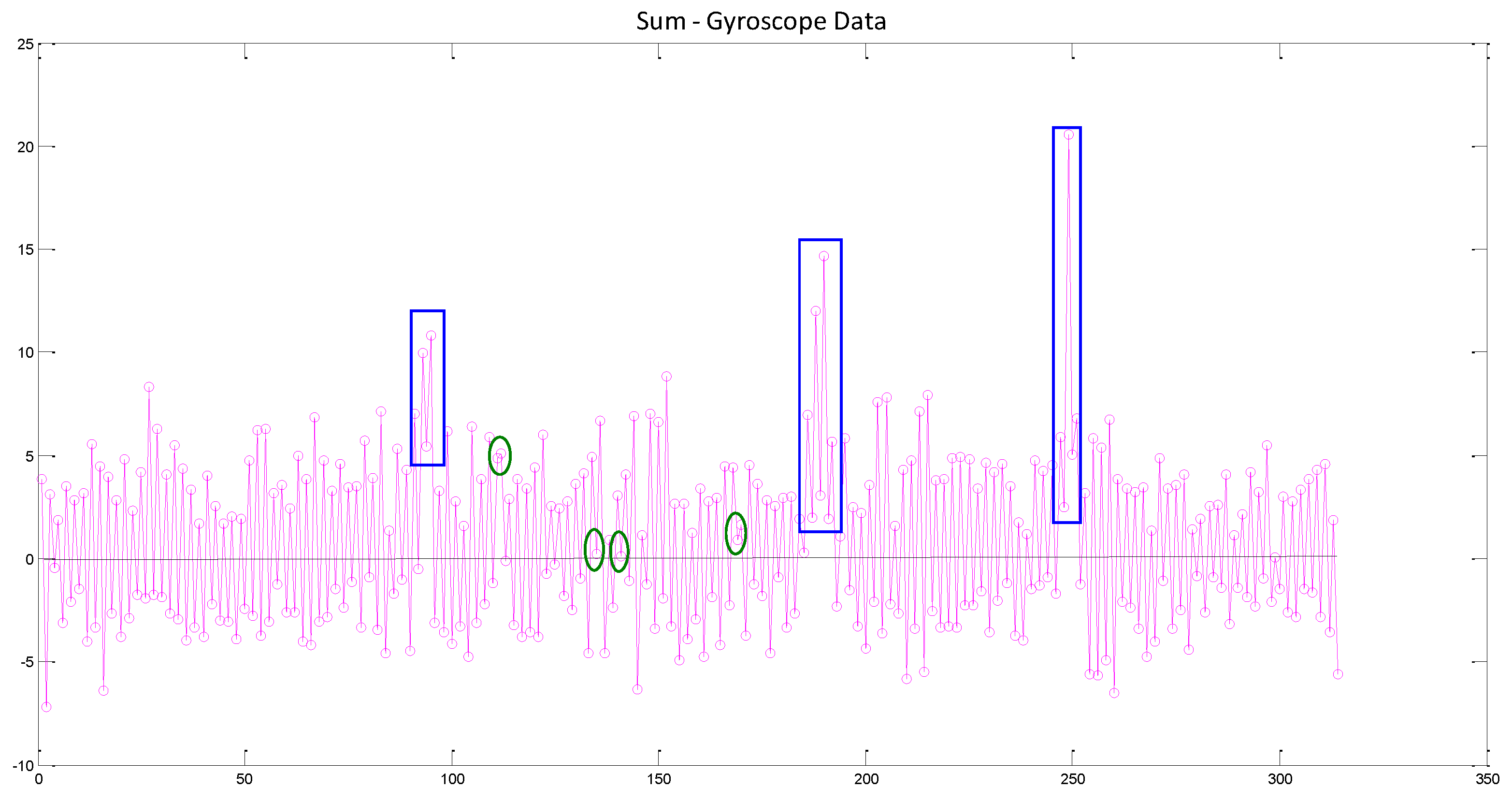
3.2. Adaptive System Noise Filter Based on the Pedestrian’s Moving Status

Based on the idea discussed in Section 3.1, to further optimize the weights of the two positioning results, the EKF method is used for fusion. Actually, our fusion method has the advantage of being able to perform a fusion calculation through the adaptive identification of the dynamic noise in the filtering system according to the pedestrian’s moving status (walking forward, turning a corner, or pseudo turning a corner) to realize a smaller trajectory divergence at the corner while improving positioning accuracy.

First, judge the stationary or moving state according to the acceleration data in the inertial measurement. In the initial positioning, gross error elimination is performed in the Wi-Fi positioning result when pedestrians stand still for a few seconds. Then, calculate the average value as the starting position of PDR. The fusion algorithm takes the position error, displacement distance difference and course error as the state variable of the filter system:

$$X=\left[dN,dE,ds,d\theta \right]$$

(10)

where N and E represent the coordinates of the positioning system in the north and east, respectively, obtained in real time; s is the step value calculated by the PDR algorithm in real time; and θ is the course angle in the moving direction. When the Wi-Fi system position is updated, the position difference between the Wi-Fi and PDR systems will be taken as the observed value of the system; namely,

$$Z={\left[\Delta N,\Delta E\right]}^T={\left[N_{w,k}-N_{p,k},E_{w,k}-E_{p,k}\right]}^T$$

(11)

where $\left(\Delta N,\Delta E\right)$ represents the position difference between the two systems at time point k, $\left(N_{w,k},E_{w,k}\right)$ is the positioning result of the Wi-Fi system at time point k, and $\left(N_{p,k},E_{p,k}\right)$ is the position information at time point k calculated according to the dead reckoning principle.

The state equation of the EKF system is

$$\{\begin{array}{l}d{N}_{k+1}=d{N}_k+\cos {\theta }_k\times d{s}_k-s_k\times \sin {\theta }_k\times d{\theta }_k+d{w}_N\\ d{E}_{k+1}=d{E}_k+\sin {\theta }_k\times d{s}_k+s_k\times \cos {\theta }_k\times d{\theta }_k+d{w}_E\\ d{s}_{k+1}=d{s}_k+d{w}_s\\ d{\theta }_{k+1}=d{\theta }_k+d{w}_{\theta }\end{array}$$

(12)

here the dynamic noise satisfaction of the position coordinates and displacement meets the Gaussian distribution—namely, $w_{N }~N\left(0,{\delta }_N^2\right)$, $w_{E }~N\left(0,{\delta }_{\mathrm{E}}^2\right)$, $w_{s }~N\left(0,{\delta }_s^2\right)$.

State-transition matrix:

$${\Phi }_k=\left[\begin{array}{cccc}1& 0& \cos {\theta }_k& -s_k\times \sin {\theta }_k\\ 0& 1& \sin {\theta }_k& s_k\times \cos {\theta }_k\\ 0& 0& 1& 0\\ 0& 0& 0& 1\end{array}\right]$$

(13)

Measurement matrix:

$$H_k=\left[\begin{array}{l}\begin{array}{cccc}1& 0& 0& 0\end{array}\\ \begin{array}{cccc}0& 1& 0& 0\end{array}\end{array}\right]$$

(14)

For the dynamic noise sequence and measurement noise sequence required in the filtering process, many positioning result data are used to obtain the experience numbers via characteristic analysis of the error statistics of the Wi-Fi and PDR positioning systems. The dynamic noise matrix is:

$$Q_k=\left[\begin{array}{cccc}{\delta }_N^2& 0& 0& 0\\ 0& {\delta }_E^2& 0& 0\\ 0& 0& {\delta }_s^2& 0\\ 0& 0& 0& {\delta }_{\theta }^2\end{array}\right]$$

(15)

Given ${\delta }_N^2={\delta }_E^2=2$, ${\delta }_s^2=1$, measurement noise matrix:

$$R=\left[\begin{array}{l}\begin{array}{cccc}Rw& 0& 0& 0\end{array}\\ \begin{array}{cccc}0& Rw& 0& 0\end{array}\end{array}\right]$$

(16)

where $R_w={10}^2$. Considering the actual situation in which the value of the course $w_{\theta }$ is larger when turning and smaller when moving straight, adaptively determine the dynamic noise value of the course-related variables by judging the pedestrian movement attributes (straight or turning). Use the accumulated value SGyr (rad/s) of the gyro data in each step to determine the movement attributes of mobile users. The judgement conditions of turning are

$$SGy{r}_k\times SGy{r}_{k-1}>0\text{ and }abs(SGy{r}_k)>10rad/s$$

(17)

In the experiment, we found that the results will improve if we dynamically adjust the Q matrix each time there are turning trends. The turning trends contain the true turning and pseudo turning, which is caused by the large deviation that occurs when a pedestrian holds the phone in a certain direction while walking. The formula for judging the turning tread is:

$$SGy{r}_k\times SGy{r}_{k-1}>0$$

(18)

When the pedestrian moves straight, ${\delta }_{\theta }^2={\left(2^{°}\right)}^2$; when the pedestrian turns, ${\delta }_{\theta }^2={\left({15}^{°}\right)}^2$; when the pedestrian moves straight but pseudo turning is caused by a slight turning of the hand, ${\delta }_{\theta }^2={\left(8^{°}\right)}^2$.

In the case in which the Wi-Fi position has not been updated, take the difference between the coordinates predicted by the system and the coordinates observed through the PDR method as the observation variables to perform a recursive correction on the calculation of the position through PDR with all others remaining unchanged:

$$Z={[\Delta N,\Delta E]}^T={[N_{k+1}-N_{p,k+1},E_{k+1}-E_{p,k+1}]}^T$$

(19)

where the coordinates predicted by the system can be updated through the following approach:

$$\begin{array}{l}{N}_{k+1}=N_{p,k}+dN+(s_k+d{s}_k)\times \cos ({\theta }_k+d{\theta }_k)\\ E_{k+1}=E_{p,k}+dE+(s_k+d{s}_k)\times \sin ({\theta }_k+d{\theta }_k)\end{array}$$

(20)

According to the position error obtained through the filtering, Formula (20) is able to update the pedestrian’s current position, which is also the final position at moment k + 1 obtained after the computation is performed in the fusion model.

4. Experimental Analysis

The experimental site was set up on the fourth floor of the School of Environment Science and Spatial Informatics, China Mining University of Technology. A Wi-Fi network system was established, and the Samsung Galaxy Note 3 (SM-N9002) was chosen as the mobile testing device. As shown in Figure 1, D-LINK wireless routers (DIR-600NB) were installed every 9 m along both sides of the corridor, providing 64 APs in total. In the positioning process, the positioning system sent the positional information to mobile users every 2 s according to the Wi-Fi signal strength. The data sampling frequency of the inertial sensor was 50 Hz; each new data point was analyzed, including the gait detection, step-size calculation, course rough calculation, and position calculation. The position was calculated according to the fusion model described in Section 3 with the Wi-Fi positioning results and PDR positioning results. In the experiment, the pedestrian started from the west end of Area C in the School of Environment Science and Spatial Informatics towards the westernmost end of Area B via Area A along the corridor at a constant speed. In this process, the pedestrian basically held the mobile phone level and walked 316 steps in total.

Figure 1. Experimental site. (a) Floor scene graph of the fourth floor; (b) 3D model of the experimental site.

Figure 1. Experimental site. (a) Floor scene graph of the fourth floor; (b) 3D model of the experimental site.

4.1. Wi-Fi Positioning Analysis

The experimental site was set up in a long, narrow corridor environment divided into A, B and C zones, and a regular quadrilateral (1.2 m × 1.2 m) grid structure was used to lay out the fingerprint points to achieve offline fingerprint data acquisition and construct the fingerprint database. The sampling rate of the device to the received signal is 100 Hz, and relevant data collected by the RPs usually includes Wi-Fi signal strength and the real coordinates of RPs. The received signal strength is an integer in (−110, −15); 390 efficient points are finally collected from the fingerprint point distribution, as shown in Figure 2 [34].

Figure 2. Distribution of fingerprint points.

Figure 2. Distribution of fingerprint points.

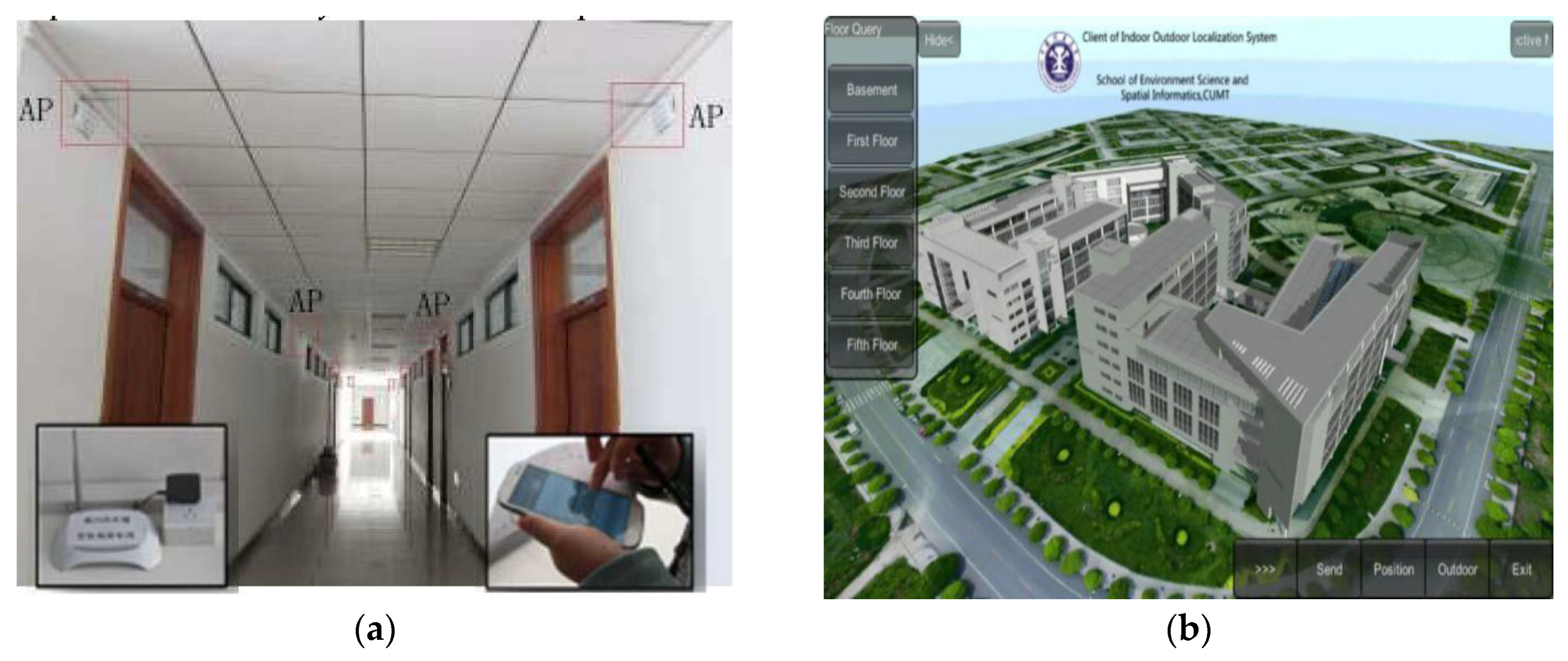
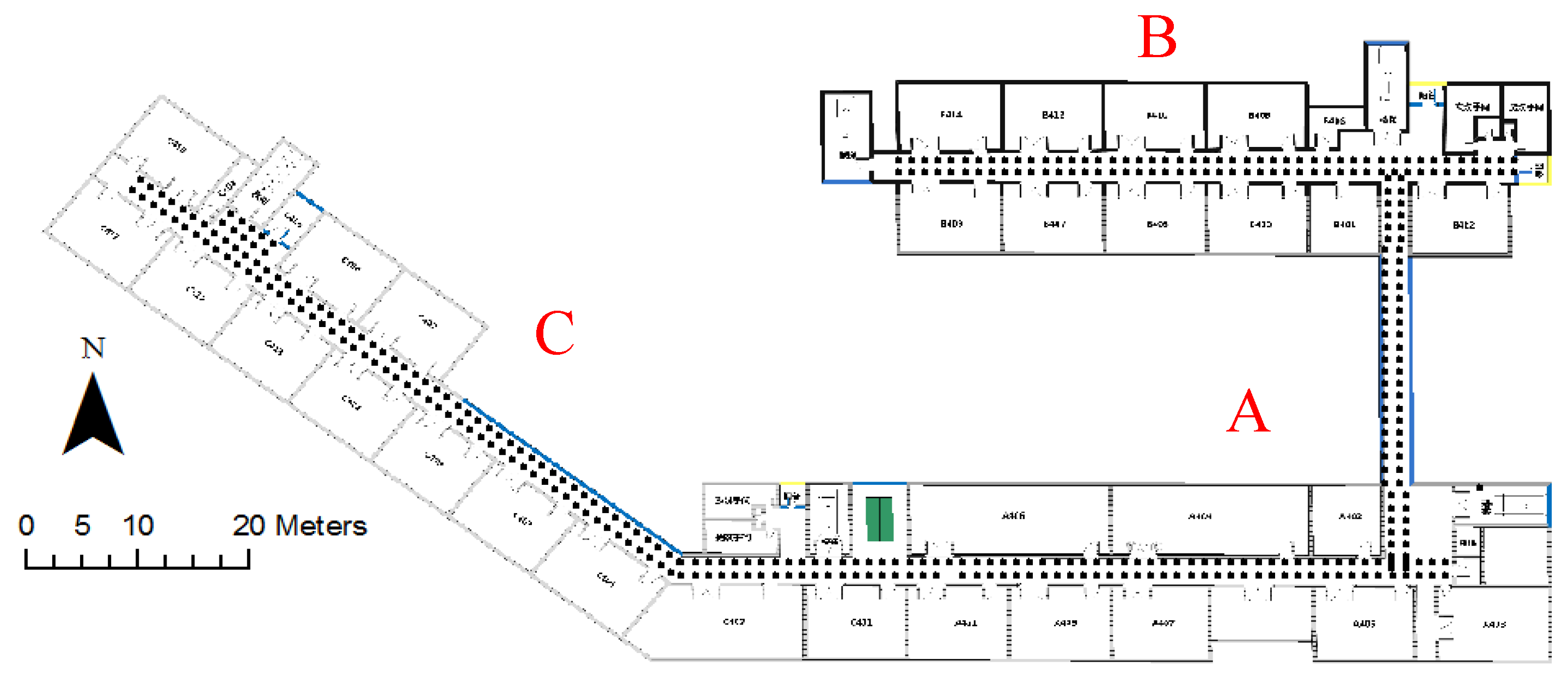
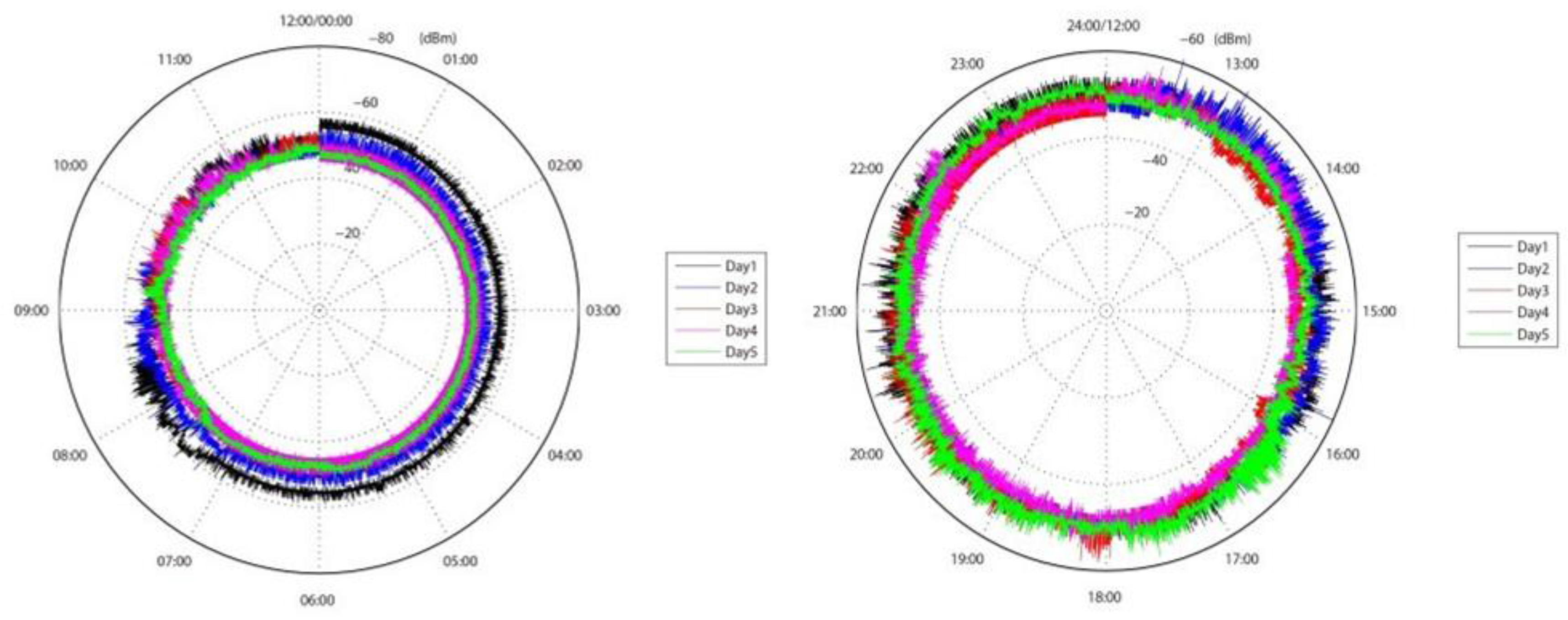
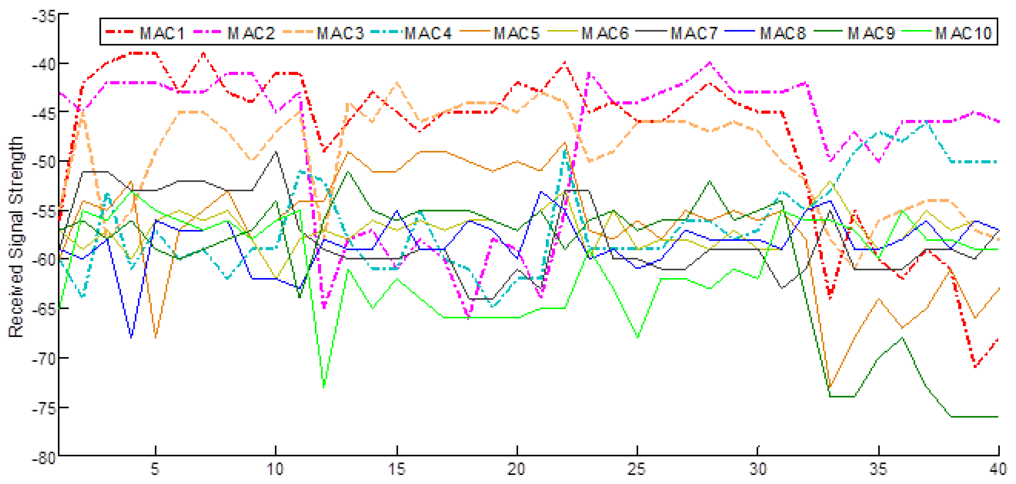
(1) Offline data acquisition and preprocessing

The Wi-Fi signal from the D-LINK (DIR-600NB) wireless router was recorded in a fixed position on the fourth floor for five days to describe the time-variation effect of the Wi-Fi signal with the measured data. The statistical results are shown in Figure 3.

Figure 3. The polar coordinates diagram for statistical results of the Wi-Fi signal in the five consecutive days.

Figure 3. The polar coordinates diagram for statistical results of the Wi-Fi signal in the five consecutive days.

From the figure, we can see that the signal propagation was stable from 23:00 to 7:00 but fluctuated greatly from 7:00 to 23:00. In fact, there were staff members in the lab beginning at 7:00, and the lab closed at 23:00. Thus, we can see that the signal is significantly affected by human disturbance. In addition, by comparing the data from the five days, we can find that the RSSI of the curves at the same time every day are different by up to 15 dB. In Wi-Fi fingerprint positioning, the fingerprint collection is distributed based on the current signal strength; the signal changes at different times in the same day, and changes in the same period on different days will result in a failure to completely describe the signal strength distribution by the statistics of the signal strength collected in one period, which will undoubtedly affect the positioning results.

Therefore, we collected fingerprint data on 10 consecutive days from 11 to 20 April 2015. Ten samples were collected in four directions by each RP each day, resulting in 40 groups of signal strength measurements in total. Figure 4 shows the signal strength information of 10 APs observed on an RP, and all 40 signals of each AP are very unstable. The data were collected from four directions because there are large differences in the signal strength values obtained in different directions at the same position. Figure 5 shows the signal strength distribution of the same AP collected by an RP in four directions (absolute value), where the maximum difference is up to 20 dBm. The measurement of difference is affected by the multipath effect caused by the layout of the environment. Moreover, the body itself is one of the important factors interfering with wireless signal propagation. Finally, the mean value of all field strengths in the four directions collected over 10 days is taken as the fingerprint information of the RP.

Figure 4. Signal strength data of 10 available APs for an RP.

Figure 4. Signal strength data of 10 available APs for an RP.

Figure 5. Signal strength observed from four sampling directions.

Figure 5. Signal strength observed from four sampling directions.

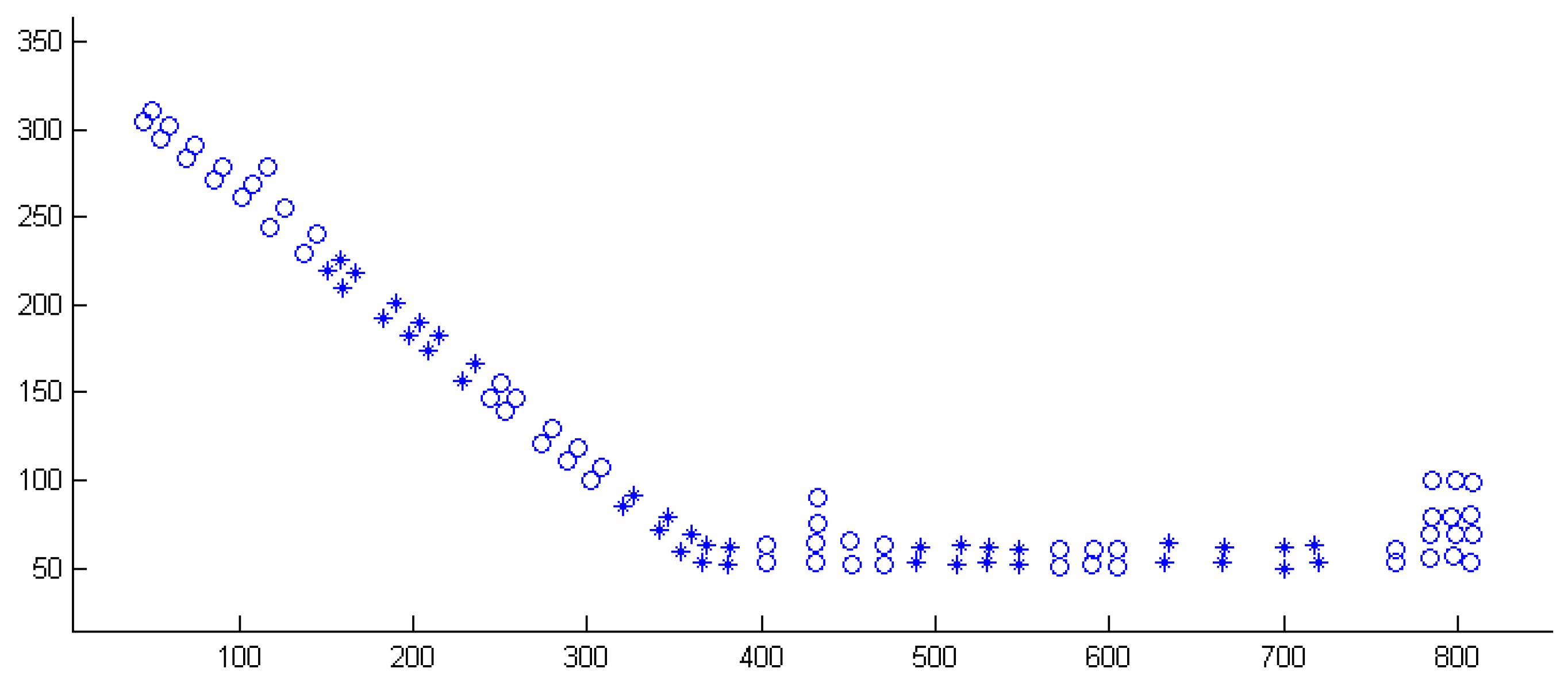
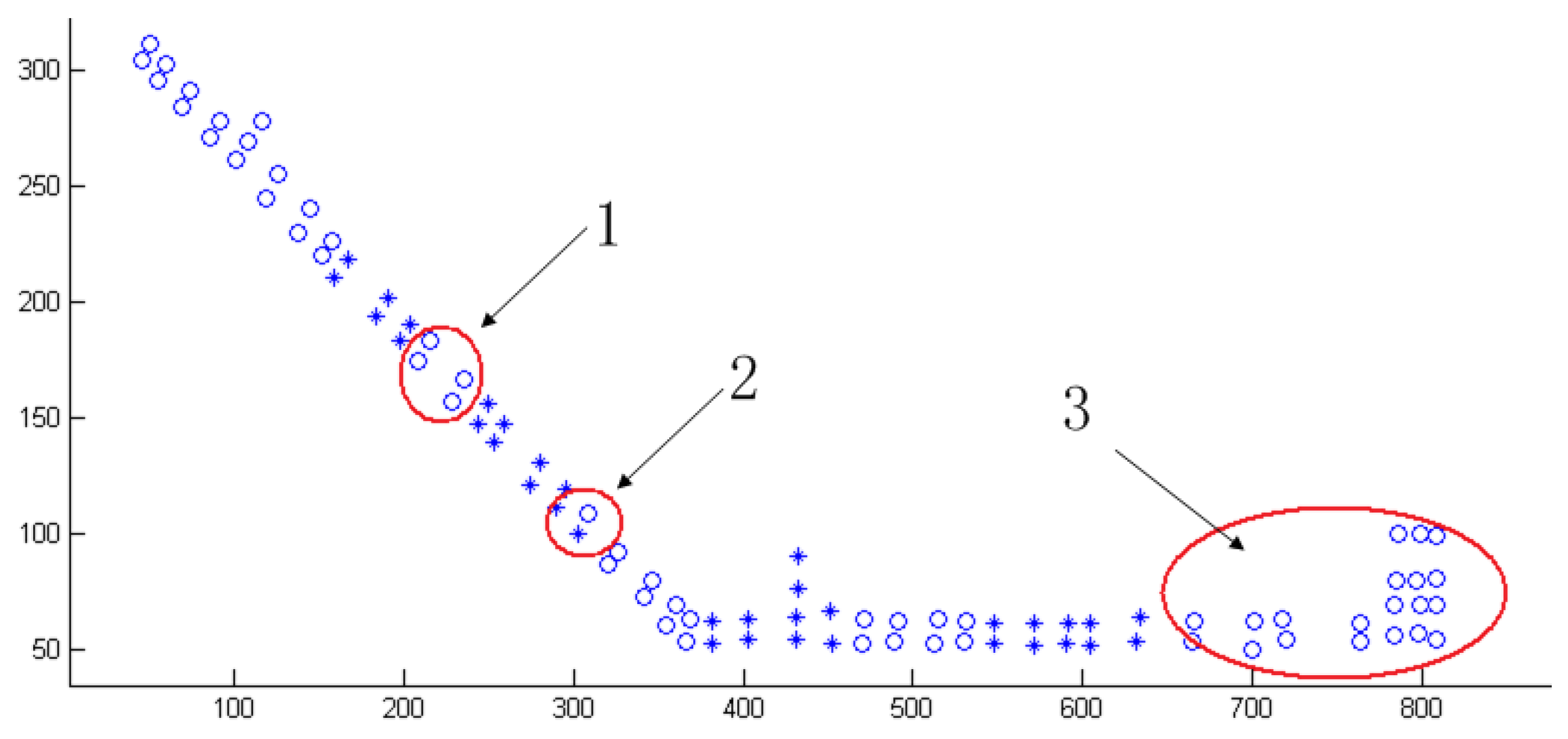
(2) Clustering analysis

To show the analysis results, the experiment re-collected 93 efficient points in Areas C and A with an average sampling interval of 3.5 m; the APC algorithm is adopted to cluster the respective points in the sample database by extracting the fusion feature.

By comparing Figure 6 and Figure 7, it can be found that the results obtained by APC clustering are closer to the geographic division, such as the corner of the corridor and the open area, and the classification results are more uniform. This is because the clustering feature in the APC method fused part of the geographic information. Although the center distance has increased, the distance control later has an important role in the improvement of the positioning accuracy.

The selection of the K-means clustering initial value is random, so the results generated by several operation iterations are different. Because the APC algorithm is an unsupervised classification method, it is unnecessary to set the number of classes and the random initial value, which is the result of long-term feedback. Therefore, the obtained calculation result is unique. The K-means classification results are shown in Figure 7. The circles are the positions with unreasonable classification: 1 is due to few class members; 2 is because of fuzzy boundaries, and 3 is because the corner of the corridor is not classified. Table 1 shows the result statistics after the K-means clustering algorithm was run 10 times.

Figure 6. APC classification results.

Figure 6. APC classification results.

Figure 7. Classification results of K-means.

Figure 7. Classification results of K-means.

Table 1. The statistics for the number of class members in the result of K-means clustering (10 times).

Times	Class 1	Class 2	Class 3	Class 4	Class 5	Class 6	Class 7	Class 8	Class 9
1	17	15	10	7	6	8	10	11	9
2	17	15	10	7	9	15	8	3	9
3	17	6	10	12	10	8	10	11	9
4	11	6	6	10	9	7	9	15	20
5	8	9	6	10	12	10	8	10	20
6	17	6	10	9	7	9	15	11	9
7	17	6	10	9	7	6	8	10	20
8	9	9	14	10	7	9	15	11	9
9	8	9	6	10	12	10	18	11	9
10	32	13	10	8	10	8	3	5	4

Table 1. The statistics for the number of class members in the result of K-means clustering (10 times).

Times	Class 1	Class 2	Class 3	Class 4	Class 5	Class 6	Class 7	Class 8	Class 9
1	17	15	10	7	6	8	10	11	9
2	17	15	10	7	9	15	8	3	9
3	17	6	10	12	10	8	10	11	9
4	11	6	6	10	9	7	9	15	20
5	8	9	6	10	12	10	8	10	20
6	17	6	10	9	7	9	15	11	9
7	17	6	10	9	7	6	8	10	20
8	9	9	14	10	7	9	15	11	9
9	8	9	6	10	12	10	18	11	9
10	32	13	10	8	10	8	3	5	4

It can be seen from Table 1 that there are great differences between the classification results under the action of different initial values, which illustrates that instability results when using K-means to cluster the respective points in the fingerprint database. Moreover, the classification number should be set before processing, which is more difficult for Wi-Fi signals, which are susceptible to interference.

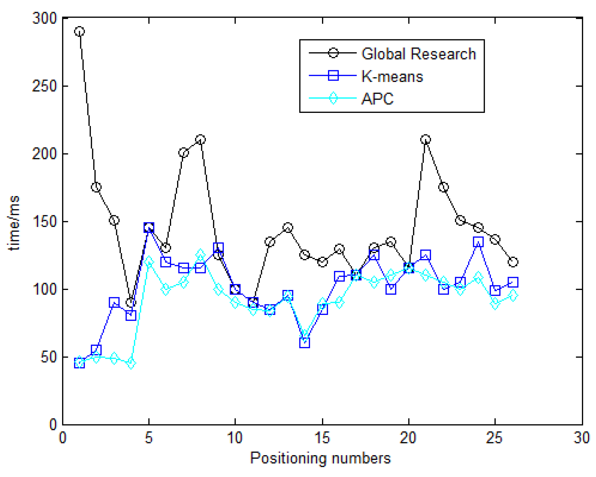
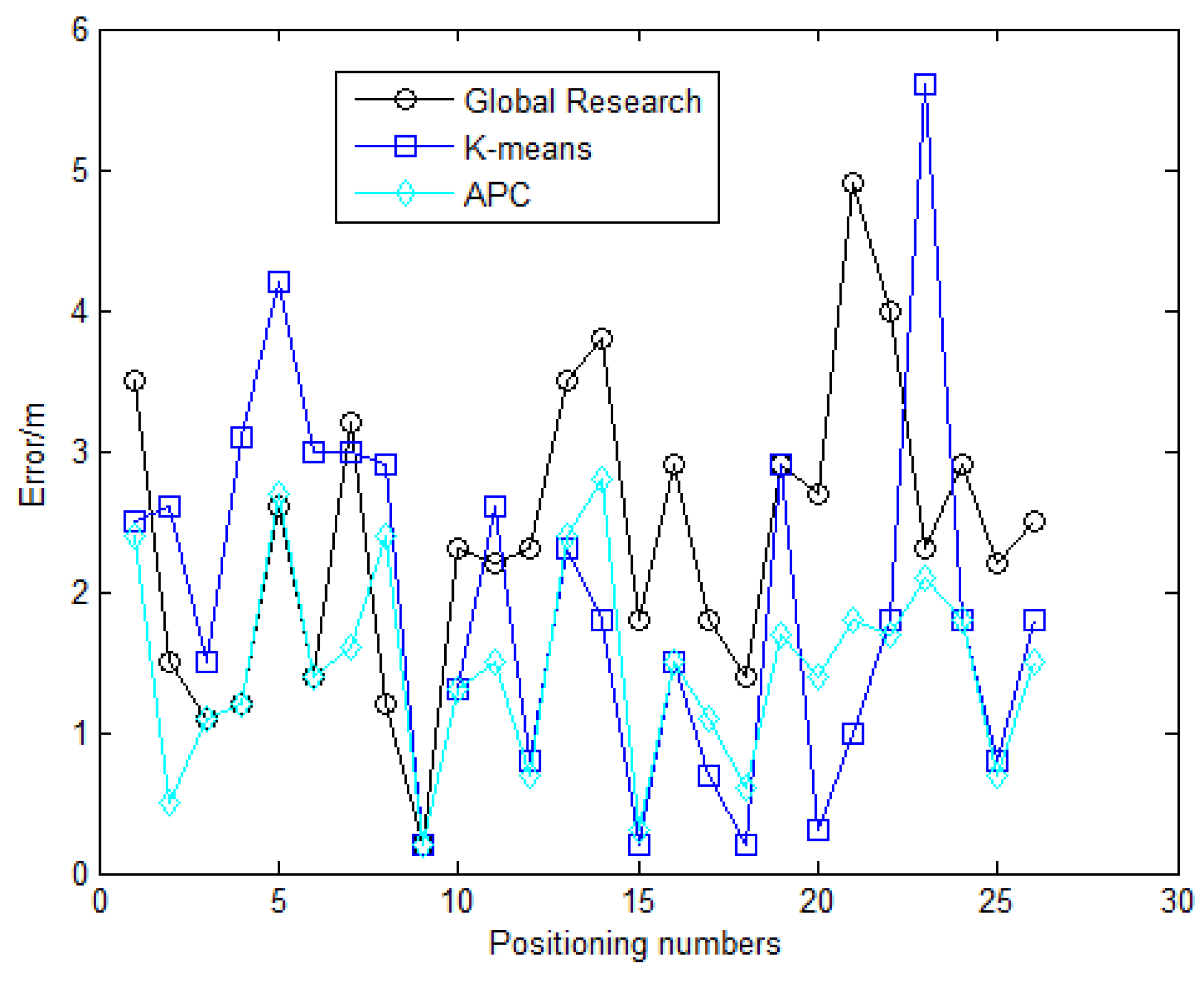
(3) Analysis results of static positioning

Static positioning test method: take 26 points to be positioned in the experimental site; sample for 10 s at the points to be positioned in the up, down, left, and right directions with the same device; and record the mean value of the Wi-Fi signal data. The experiment analyzes and compares the positioning effects of APC and K-means from the aspects of time efficiency and positioning accuracy. The positioning times of the 26 points to be positioned are shown in Figure 8. After the clustering process, both the data search volume and positioning time are reduced. Compared with a global search, K-means and APC clustering processing achieve great improvement in time efficiency. The average positioning time of global search is 127 ms, and K-means and APC have similar effects, which are 76 ms and 70 ms, respectively. The largest drop by K-means is 88.2%, and the smallest drop is only 0.2%, whereas the largest drop by APC is 87.2%, and the smallest drop is up to 16.8%. The quantity of data searched by APC decreases by 75% on average and 80% at most. Because the average reduction rates of APC and K-means are almost the same, the average positioning time of the two clustering methods is similar; however, K-means has a larger drop because of the great difference in the numbers of sampling points searched on each positioning point caused by the non-uniformity of the clustering results.

Figure 8. Comparison of static positioning time.

Figure 8. Comparison of static positioning time.

As shown in Figure 9, the clustered positioning result is more accurate than that of the global search. The average positioning accuracy of the global search is 2.6 m, but the positioning accuracies of K-means and APC are 1.6 m and 1.5 m, respectively; the maximum positioning error of K-means is 5.6 m, and the minimum positioning error is 0.18 m; the maximum positioning error of APC is 2.8 m, and the minimum positioning error is 0.2 m. In terms of the average error, APC has a slightly better result than K-means and has a smaller error fluctuation. The class with few members in the K-means, combined with the fact that the mean value of the signal of that class cannot reflect the features of this kind of area signal, can easily result in mismatching and thus reduce the accuracy.

Figure 9. Comparison of static positioning accuracy.

Figure 9. Comparison of static positioning accuracy.

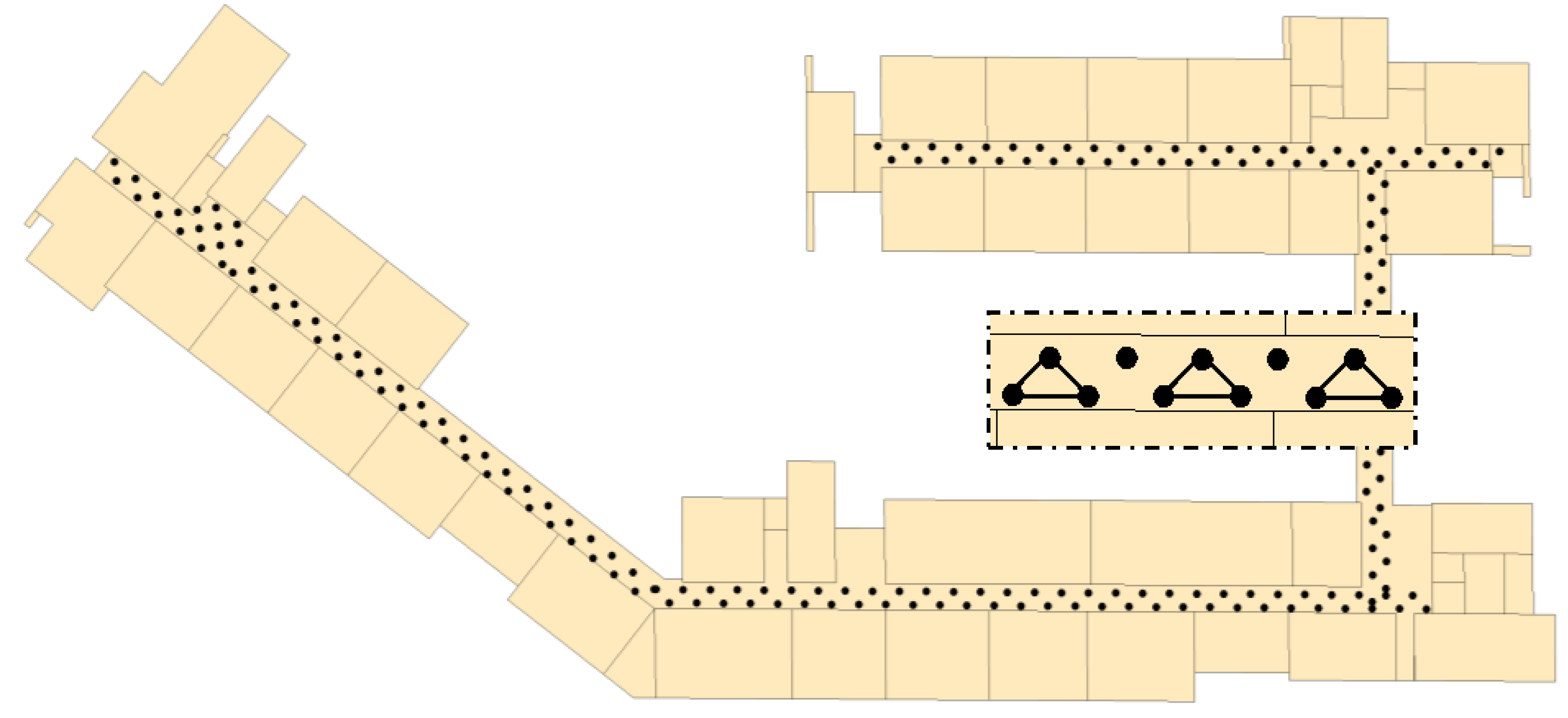
(4) Triangle mesh structure of fingerprint points

To further improve the computation efficiency, we attempted a triangle mesh structure layout of fingerprint points, as shown in Figure 10. There is no significant difference in the positioning accuracies of the APC clustering of the fingerprint database based on the two structural layouts. The static positioning accuracy is within 2 m on average, and the average accuracy of dynamic positioning is approximately 4 m, as shown in Table 2. However, considering the workload of the off sampling, the triangular mesh of fingerprint points is half the square grid in accordance with the layout plan of this paper; that is, compared with the quadrangular layout plan, the workload of the offline sampling is reduced by half, and the two layout plans contain 195 and 390 fingerprint points, respectively. Therefore, the triangular mesh fingerprint reference points can be set in the environment with long and narrow features for the collection of Wi-Fi fingerprint data.

The inconsistency of dynamic and static positioning accuracy is caused by the static positioning data, consisting of the mean value of multi-data collected from four directions, so the positioning accuracy is higher; however, the Wi-Fi dynamic positioning data are collected by the device in real time, which only uses a group of scanning data. That is, when the signal scanned by the device is changed or updated, the new data are used immediately for the positioning calculation. Owing to the randomness and the instability of the signal, the positioning accuracy is lower than the static data position calculation.

Figure 10. Triangular mesh structure layout of fingerprint points.

Figure 10. Triangular mesh structure layout of fingerprint points.

Table 2. Positioning results based on different layout fingerprint databases.

	Quadrilateral fingerprint database	Triangle fingerprint database
Average error of static positioning / m	1.50	1.76
Maximum error of static positioning / m	2.80	3.52
Average error of dynamic positioning / m	4.09	4.43
Maximum error of dynamic positioning / m	19.76	22.4

Table 2. Positioning results based on different layout fingerprint databases.

	Quadrilateral fingerprint database	Triangle fingerprint database
Average error of static positioning / m	1.50	1.76
Maximum error of static positioning / m	2.80	3.52
Average error of dynamic positioning / m	4.09	4.43
Maximum error of dynamic positioning / m	19.76	22.4

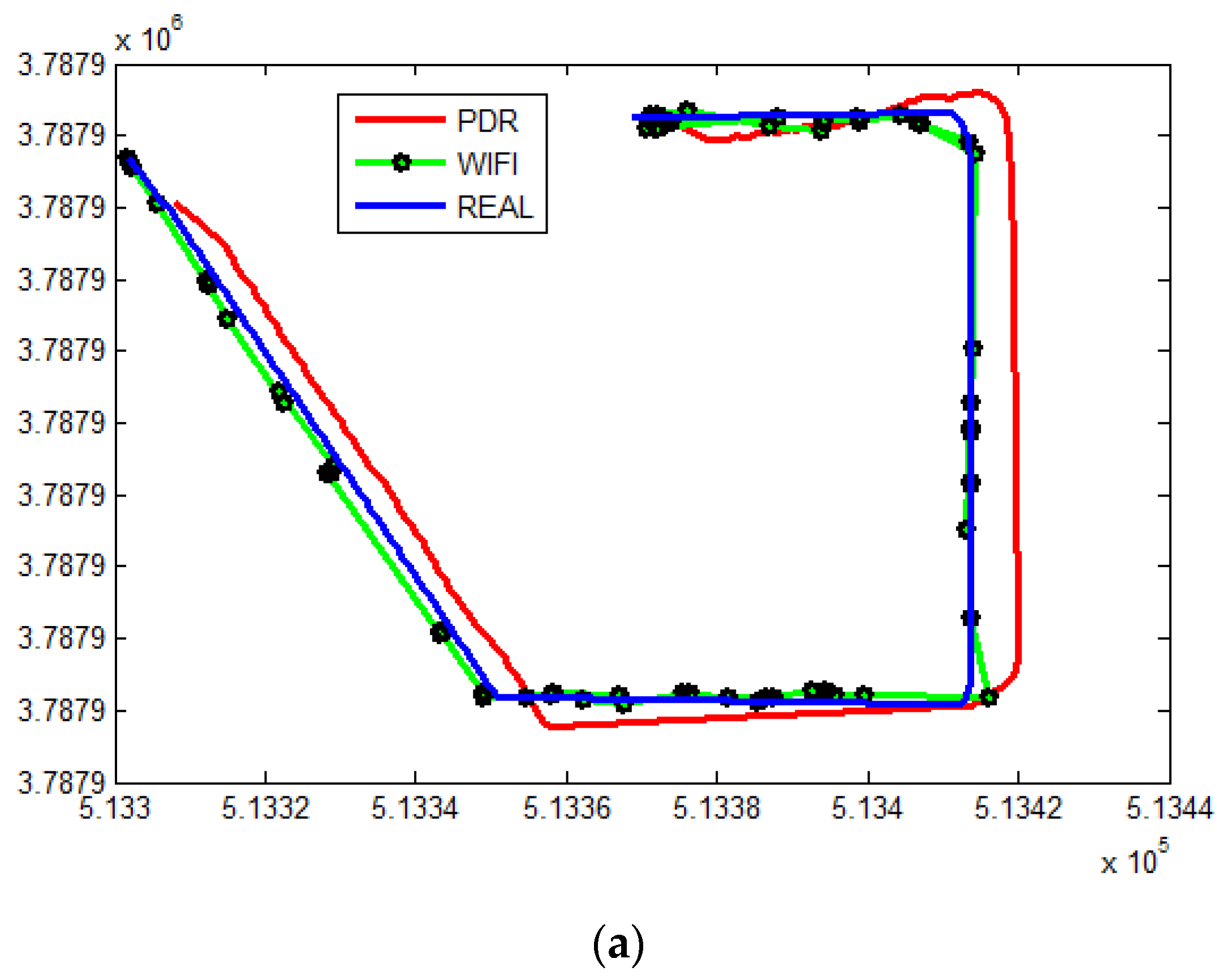
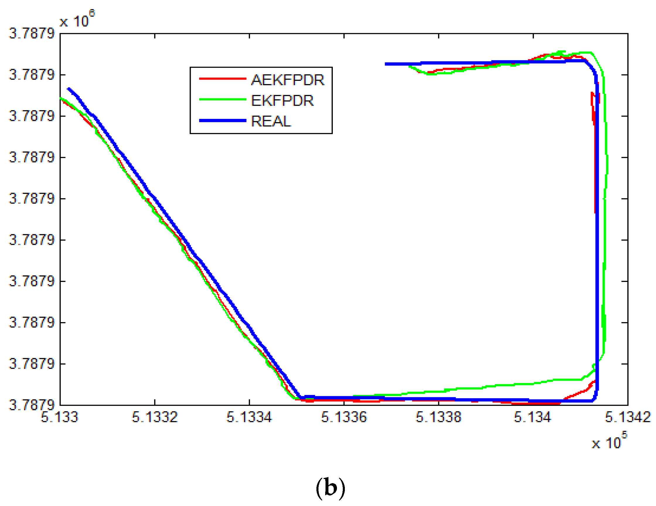
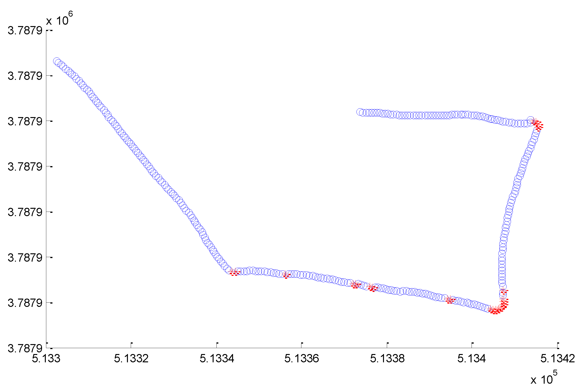
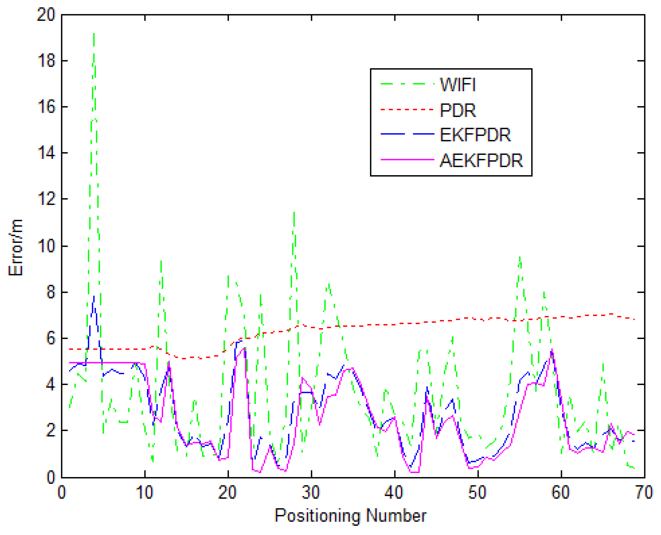
4.2. Fusion Analysis

Because the Wi-Fi positioning system has an absolute positioning function, the positioning results of the system can be considered as the PDR initial point. By calculation, the initial position error of the quadrilateral fingerprint database positioning is 2.58 m, which uses four kinds of positioning schemes for the indoor positioning test:

Scheme 1: Using the WKNN positioning model based on a Wi-Fi signal strength affinity clustering fingerprint database to mark Wi-Fi.

Scheme 2: With the Wi-Fi static smooth positioning results as the starting point, mark the PDR positioning based on compensation course reckoning as PDR. Here, the estimation of course error is based on the method proposed by Chen in 2010 [35].

Scheme 3: According to the Wi-Fi positioning and course correction PDR, mark WEPDR based on conventional EKF value fusion positioning.

Scheme 4: According to the Wi-Fi positioning and course correction PDR, mark AWEPDR based on the fusion positioning of the adaptive model noise extended Kalman filter.

The trajectory of positioning results obtained by the different positioning models is shown in Figure 11.

For the user trajectory of the Wi-Fi positioning system in Scheme 1, two apparent instabilities are shown in the figure: first, there are many occasions of the rebound phenomenon (according to the user moving direction in this experiment, the normal movement trajectories can be only forward along the route). The concept of “rebound” in this paper characterizes the received rear position information fed back by the system in the forward positioning; second, there are repeated accumulation points in positioning. That is, the user received feedback of the same position or a nearby position in different positions at different time points, which caused the clustering of positioning points. It is found that those two issues are a large problem independently based on the Wi-Fi signal fingerprint database positioning algorithm.

Figure 11. Trajectory analysis for different indoor positioning methods. (a) Trajectory of PDR, WIFI,REAL; (b) trajectory of AEKFPDR, EKFPDR.

Figure 11. Trajectory analysis for different indoor positioning methods. (a) Trajectory of PDR, WIFI,REAL; (b) trajectory of AEKFPDR, EKFPDR.

In Scheme 2, owing to the error of gait detection, step-size calculation, and course estimation, there are some errors with the PDR positioning results. Owing to the error of the initial position obtained by Wi-Fi positioning, the position of the overbridge from Area B to Area A especially deviates from the structures. However, its advantage is that the output positioning points are uninterrupted, and there is no rebound or clustering phenomenon.

In Scheme 3, the point positions are evenly distributed, and there is little rebound, which alleviates the pileup problems to some degree. It can be seen that the classic EKF fusion algorithm preserves the continuity and short-term stability of the pedestrian dead reckoning, which greatly weakens the error accumulation of the PDR and has a certain capability to resist the gross Wi-Fi error. With the increasing fusion times, the deviated points will gradually return to the real track trajectory direction. Although the initial positioning error is approximately 4.2 m, the positioning accuracy can be gradually compensated to some degree with the update of Wi-Fi positions. However, the divergence problem of point positions still exists at the corners.

In Scheme 4, the noise matrix value Q is dynamically set according to the pedestrian movement attributes (straight or turning). Figure 12 shows the accumulated gyro value corresponding to each step of the pedestrian, in which the singular points in the three rectangular boxes represent the three occasions of true turning of the mobile users, and the other four points marked with ellipses are “pseudo-turning.” There are seven “turning trends” on the routes in total, marked with a red circle in Figure 13.

Figure 12. Analysis of the accumulated gyro value.

Figure 12. Analysis of the accumulated gyro value.

Figure 13. Analysis of the accumulated gyro value.

Figure 13. Analysis of the accumulated gyro value.

The experimental results show that the convergence speed at corners in Scheme 4 is higher than that of the classic EKF. While maintaining the stability and the strong ability to resist Wi-Fi gross error and other advantages, Scheme 4 also weakens the divergence at the corners while improving the positioning accuracy.

The detailed error analysis of the four different schemes in Figure 14 and Table 3 shows that the average positioning error of AWEPDR is the smallest and accounts for 56.2%, 37.5%, and 85.9% of the average error values of the other three models. The maximum average positioning error of AWEPDR accounts for 26.8%, 81.2%, and 66.4%, and the minimum positioning error accounts for 55.8%, 4.2%, and 78.4% of the other three models.

Figure 14. Error analysis of different indoor positioning methods.

Figure 14. Error analysis of different indoor positioning methods.

Table 3. Error analysis of different indoor positioning methods.

	Wi-Fi	PDR	WEPDR	AWEPDR
Minimum error/m	0.36	5.14	0.28	0.22
Average error/m	4.09	6.08	2.74	2.32
Maximum error/m	19.35	6.46	7.96	5.25

Table 3. Error analysis of different indoor positioning methods.

	Wi-Fi	PDR	WEPDR	AWEPDR
Minimum error/m	0.36	5.14	0.28	0.22
Average error/m	4.09	6.08	2.74	2.32
Maximum error/m	19.35	6.46	7.96	5.25

In conclusion, the indoor positioning result can be controlled within 2.5 m by adaptive noise EKF filtering fusion of Wi-Fi system positioning results and PDR, which meet the demand of pedestrian indoor navigation and positioning.

5. Conclusions

Clustering processing is performed on the fingerprint data of indoor positioning by the APC algorithm to reduce the traversal data volume in positioning and improve the positioning accuracy. Based on this, the calculation method of adaptively determining the filtering system dynamic noise to conduct the fusion calculation based on pedestrian movement (straight or turning) is proposed according to the respective advantages of Wi-Fi and PDR positioning systems. The experimental results show that the fusion algorithm can effectively solve the instability problems such as Wi-Fi positioning jumping and clustering, overcome the positioning error and cumulative error of PDR caused by the initial position error, and thus improve the reliability and robustness of indoor positioning.

References

1. Mahfouz, M.R.; Kuhn, M.J.; To, G.; Fathy, A.E. Integration of UWB and wireless pressure mapping in surgical navigation. IEEE Trans. Microw. Theory Tech. 2009, 57, 2550–2564. [Google Scholar] [CrossRef]
2. Gu, Y.; Lo, A.; Niemegeers, I. A survey of indoor positioning systems for wireless personal networks. IEEE Commun. Surv. Tutor. 2009, 11, 13–32. [Google Scholar] [CrossRef]
3. Hightower, J.; Borriello, G. Location systems for ubiquitous computing. Computer 2001, 34, 57–66. [Google Scholar] [CrossRef]
4. Li, F.; Zhao, C.; Ding, G.; Gong, J.; Liu, C.; Zhao, F. A reliable and accurate indoor localization method using phone inertial sensors. In Proceedings of the 2012 ACM Conference on Ubiquitous Computing, Pittsburgh, PA, USA, 5–8 September 2012; pp. 421–430.
5. Pahlavan, K.; Li, X.; Makela, J.-P. Indoor geolocation science and technology. IEEE Commun. Mag. 2002, 40, 112–118. [Google Scholar] [CrossRef]
6. Jimenez, A.; Seco, F.; Prieto, C.; Guevara, J. A comparison of pedestrian dead-reckoning algorithms using a low-cost MEMS IMU. In Proceedings of the 2009 IEEE International Symposium on Intelligent Signal Processing, Budapest, Hungary, 26–28 August 2009; pp. 37–42.
7. Mautz, R. The challenges of indoor environments and specification on some alternative positioning systems. In Proceedings of the 6th Workshop on Positioning, Navigation and Communication, Hannover, Germany, 19 March 2009; pp. 29–36.
8. Marano, S.; Gifford, W.M.; Wymeersch, H.; Win, M.Z. NLOS identification and mitigation for localization based on uwb experimental data. IEEE J. Sel. Areas Commun. 2010, 28, 1026–1035. [Google Scholar] [CrossRef]
9. Foxlin, E. Pedestrian tracking with shoe-mounted inertial sensors. IEEE Comput. Graph. Appl. 2005, 25, 38–46. [Google Scholar] [CrossRef] [PubMed]
10. Colomar, D.S.; Nilsson, J.; Handel, P. Smoothing for Zupt-aided INSS. In Proceedings of the 2012 International Conference on Indoor Positioning and Indoor Navigation (IPIN), Sydney, NSW, Australia, 13–15 November 2012; pp. 1–5.
11. Jiménez, A.R.; Seco, F.; Prieto, J.C.; Guevara, J. Indoor pedestrian navigation using an INS/EKF framework for yaw drift reduction and a foot-mounted IMU. In Proceedings of the 7th Workshop on Positioning Navigation and Communication, Dresden, Germany, 8 June 2010; pp. 135–143.
12. Harle, R. A survey of indoor inertial positioning systems for pedestrians. IEEE Commun. Surv. Tutor. 2013, 15, 1281–1293. [Google Scholar] [CrossRef]
13. Ruiz, A.R.J.; Granja, F.S.; Prieto Honorato, J.C.; Rosas, J.I.G. Accurate pedestrian indoor navigation by tightly coupling foot-mounted IMU and RFID measurements. IEEE Trans. Instrum. Meas. 2012, 61, 178–189. [Google Scholar] [CrossRef]
14. Adams, D. Introduction to inertial navigation. J. Navig. 1956, 9, 249–259. [Google Scholar] [CrossRef]
15. Jiménez, A.R.; Zampella, F.; Seco, F. Improving inertial pedestrian dead-reckoning by detecting unmodified switched-on lamps in buildings. Sensors 2014, 14, 731–769. [Google Scholar] [CrossRef] [PubMed]
16. Widyawan; Pirklb, G.; Munarettoc, D.; Fischerd, C.; Ane, C.; Lukowiczb, P.; Klepalf, M.; Timm-Gielg, A.; Widmerh, J.; Pesch, D.; et al. Virtual lifeline: Multimodal sensor data fusion for robust navigation in unknown environments. Pervasive Mob. Comput. 2012, 8, 388–401. [Google Scholar] [CrossRef]
17. Li, Y.; Zhang, Y.; Lan, H.; Zhang, P.; Niu, X.; El-Sheimy, N. WiFi-aided magnetic matching for indoor navigation with consumer portable devices. Micromachines 2015, 6, 747–764. [Google Scholar] [CrossRef]
18. Masiero, A.; Guarnieri, A.; Pirotti, F.; Vettore, A. A particle filter for smartphone-based indoor pedestrian navigation. Micromachines 2014, 5, 1012–1033. [Google Scholar] [CrossRef]
19. Ghinamo, G.; Corbi, C.; Francini, G.; Lepsoy, S.; Lovisolo, P.; Lingua, A.; Aicardi, I. The MPEG7 visual search solution for image recognition based positioning using 3D models. In Proceedings of the 27th International Technical Meeting of The Satellite Division of the Institute of Navigation, Tampa, FL, USA, 8–12 September 2014.
20. Saeedi, S.; Moussa, A.; El-Sheimy, N. Context-aware personal navigation using embedded sensor fusion in smartphones. Sensors 2014, 14, 5742–5767. [Google Scholar] [CrossRef] [PubMed]
21. Ling, P.; Chen, R.; Liu, J. Using Inquiry-based bluetooth RSSI probability distributions for indoor positioning. J. Glob. Position. Syst. 2010, 9, 122–130. [Google Scholar]
22. Youssef, M.A.; Agrawala, A.; Shankar, A.U.; Noh, S.H. A Probabilistic Clustering-Based Indoor Location Determination System. Available online: http://www.cs.umd.edu/~moustafa/papers/locdet_tr.pdf (accessed on 23 April 2015).
23. Yousseff, M.; Agrawala, A. Handling samples correlation in the Horus system. In Proceedings of the 23rd Annual Joint Conference of the IEEE Computer and Communications Societies, Hong Kong, China, 7–11 March 2004.
24. Yousseff, M.; Agrawala, A. Location determination via clustering and probability distributions. Pervasive Comput. Commun. 2003, 8, 143–150. [Google Scholar]
25. Shin, B.; Lee, J.H.; Lee, T.; Kim, H.S. Enhanced weighted K-nearest neighbor algorithm for indoor Wi-Fi positioning systems. In Proceedings of the 8th International Conference on Computing Technology and Information Management (ICCM), Seoul, South Korea, 24–26 April 2012.
26. Kuo, S.P. Cluster-enhances techniques for pattern-matching localization systems. Mob. Ad-Hoc Sens. Syst. 2007, 7, 1–9. [Google Scholar]
27. Bahl, P.; Padmanabhan, V.N. RADAR: An in-building RF-based user location and tracking system. In Proceedings of the 9th Annual Joint Conference of the IEEE Computer and Communications Societies, Tel Aviv, Israel, 26–30 March 2000; pp. 775–784.
28. Klingbeil, L.; Wark, T. A wireless sensor network for real-time indoor localization and motion monitoring. In Proceedings of the 7th International Conference on Information Processing in Sensor Networks, St. Louis, MO, USA, 22–24 April 2008; pp. 39–50.
29. Frey, B.J.; Dueck, D. Clustering by passing messages between data points. Science 2007, 315, 972–976. [Google Scholar] [CrossRef] [PubMed]
30. Yu, F.; Jiang, M.; Liang, J. An indoor localization of WiFi based on branch-bound algorithm. In Proceedings of the 2014 International Conference on Information Science, Electronics and Electrical Engineering (ISEEE), Sapporo, Japan, 26–28 April 2014; pp. 1306–1308.
31. Song, L.; Hatzinakos, D. A cross-layer architecture of wireless sensor networks for target tracking. IEEE/ACM Trans. Netw. 2007, 15, 145–158. [Google Scholar] [CrossRef]
32. Cho, S.Y.; Park, C.G. MEMS based pedestrian navigation system. J. Navig. 2006, 6, 135–153. [Google Scholar] [CrossRef]
33. Klepal, M.; Beauregard, S. A backtracking particle filter for fusing building plans with PDR displacement estimates. In Proceedings of the 5th Workshop on Positioning, Navigation and Communication, Hannover, Germany, 27 March 2008; pp. 207–212.
34. Chen, G.; Meng, X.; Wang, Y.; Zhang, Y.; Tian, P.; Yang, H. Integrated WiFi/PDR/Smartphone using an unscented Kalman Filter algorithm for 3D indoor localization. Sensors 2015, 15, 24595–24614. [Google Scholar] [CrossRef] [PubMed]
35. Chen, W.; Chen, R.; Chen, Y.; Kuusniemi, H.; Wang, J.; Fu, Z. An effective pedestrian dead reckoning algorithm using a unified heading error model. In Proceedings of the 2010 IEEE/ION Position Location and Navigation Symposium (PLANS), Indian Wells, CA, USA, 4–6 May 2010; pp. 340–347.