
An Assessment of Urban Surface Energy Fluxes Using a Sub-Pixel Remote Sensing Analysis: A Case Study in Suzhou, China

 ,
,
Abstract
:1. Introduction
2. Materials and Method
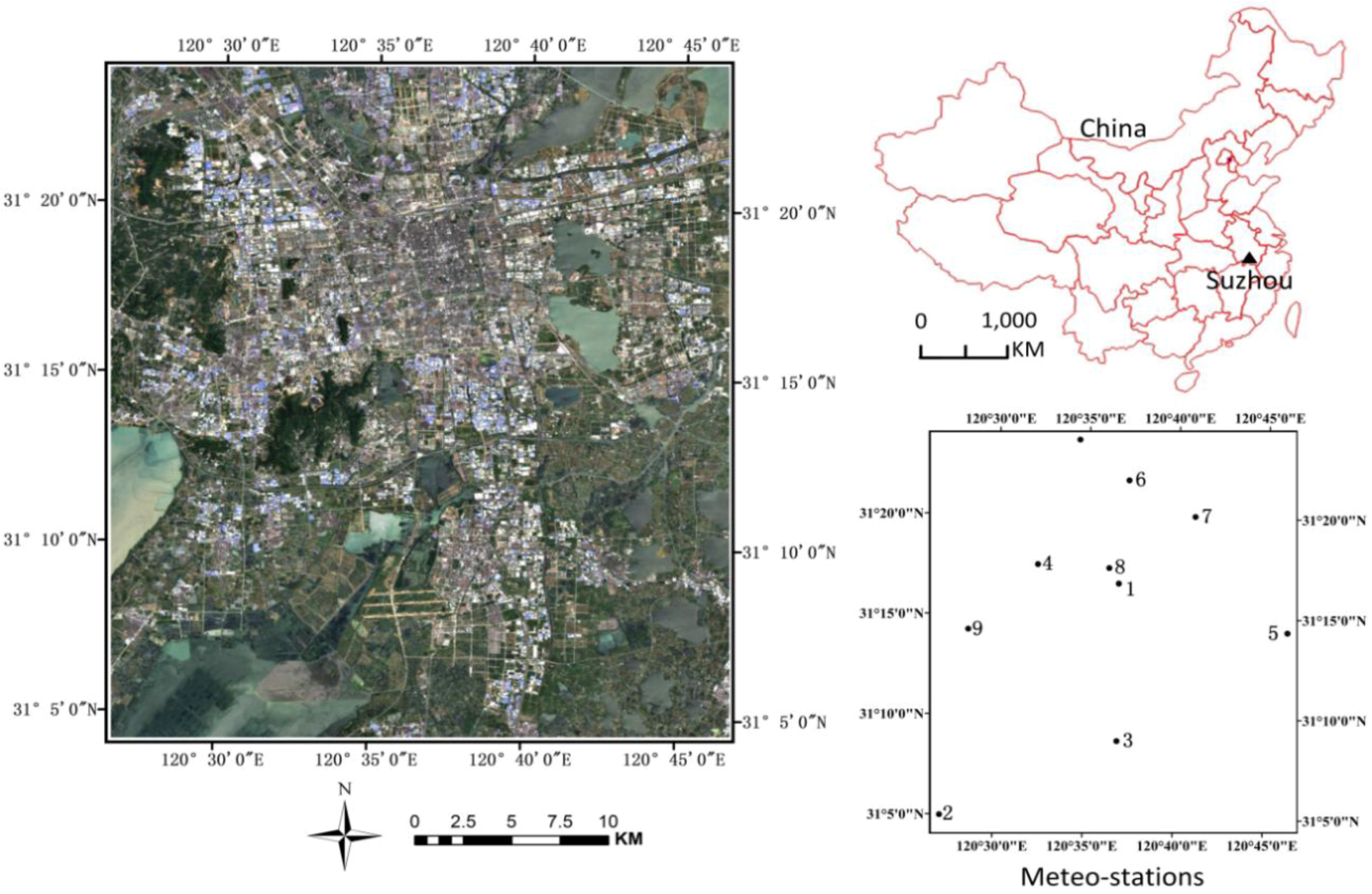
2.1. Study Area and Materials


| ID | Meteo-Stations | Latitude (degree) | Longitude (degree) | AT (°C) | WS (ms−1) | RH (%) | SSD (Hour) |
|---|---|---|---|---|---|---|---|
| 1 | Suzhou | 31.27 | 120.63 | 24.7 | 2.2 | 46.0 | 11.2 |
| 2 | Dongshan | 31.07 | 120.43 | 22.9 | 2.0 | 56.0 | 12.2 |
| 3 | Wujiang | 31.13 | 120.62 | 23.0 | 4.5 | 54.7 | 11.6 |
| 4 | Suzhou Park | 31.29 | 120.54 | 25.0 | 3.1 | ||
| 5 | Xukou Marine Firm | 31.23 | 120.47 | 23.1 | 3.5 | ||
| 6 | Xiangcheng Road | 31.37 | 120.63 | 24.5 | 3.0 | 42.7 | |
| 7 | Kuatang | 31.33 | 120.68 | 24.5 | 2.6 | ||
| 8 | Experimental Primary School | 31.28 | 120.62 | 23.9 | 1.2 | ||
| 9 | Sanmadun | 31.25 | 120.78 | 23.2 | 4.7 | ||
| 10 | Huangdi | 31.42 | 120.6 | 24.6 | 3.9 |
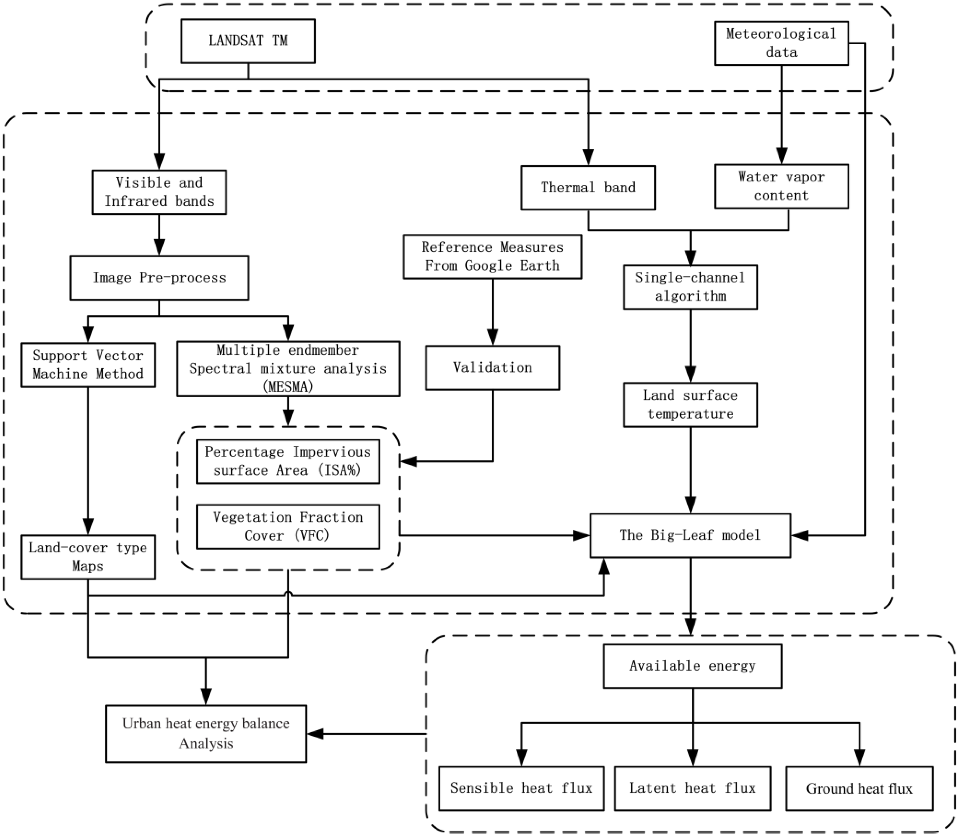
2.2. Methodology

2.2.1. Retrieving the LST
2.2.2. Retrieval of Heat Flux Components
| LCTs | |||
|---|---|---|---|
| Water | 0.3 × 10⁻⁴ | 0.34 | 0 |
| Bare soil | 0.001 | 50 | 0 |
| Crop field | 0.1 | 100 | 0.02 |
| Lawn | 0.001 | 50 | 0.133 |
| Forest | 0.5–1.0 | 1000 | 4 |
| Developed, low | 0.5 | 1000 | 2.5 |
| Developed, high | 1.5 | 1000 | 7.5 |
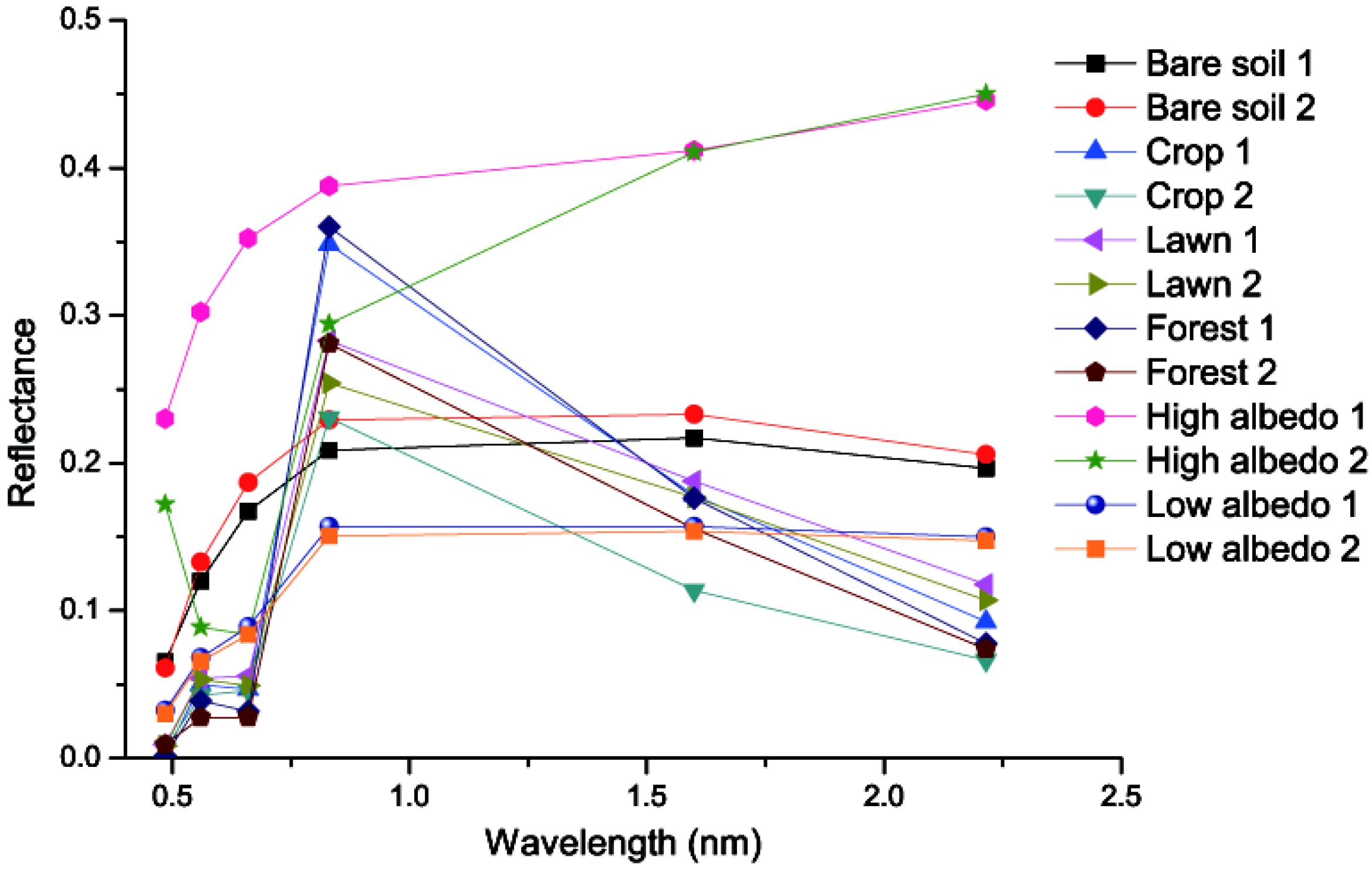
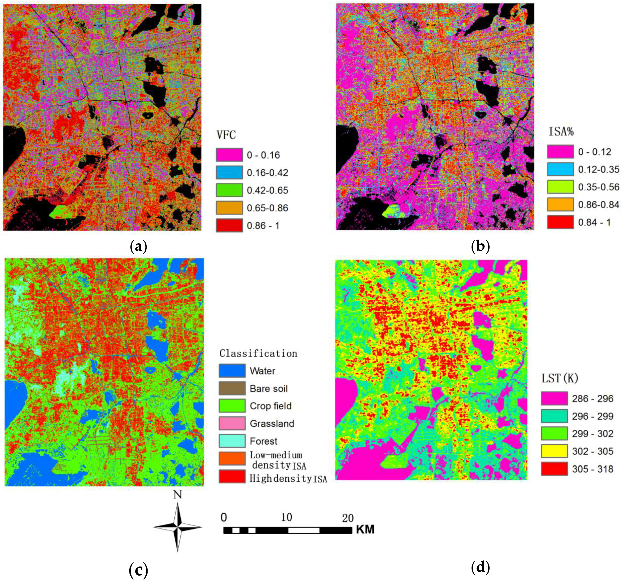
2.2.3. Retrieving the VFC, ISA% and Land Classification Map

3. Results and Discussion
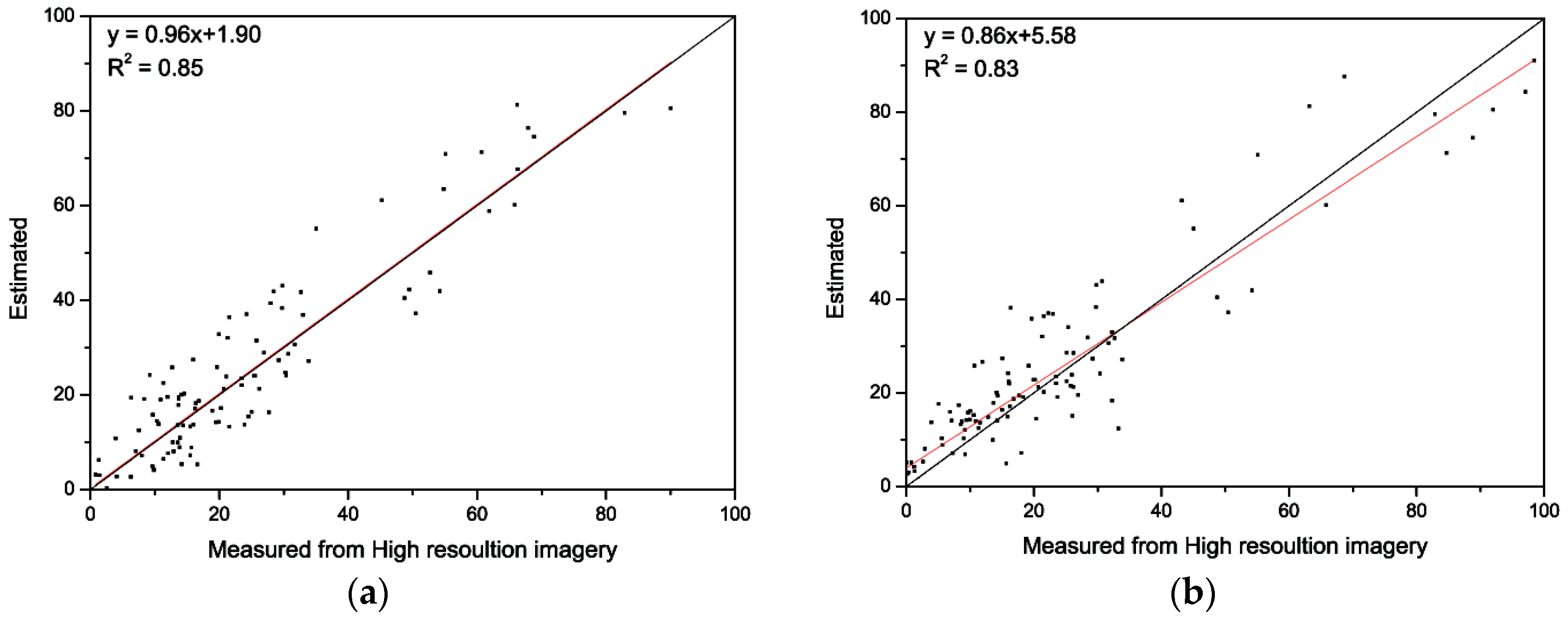
3.1. Validation of the Land Cover Fractions and Heat Fluxes


| Mean Value | H/Rn (%) | LE/Rn (%) | DG/Rn (%) |
|---|---|---|---|
| Bare soil | 3.81 | 32.5 | 63.81 |
| Crop | 5.56 | 65.6 | 33.22 |
| Lawn | 2.35 | 53.1 | 44.58 |
| Forest | 3.60 | 85.85 | 15.27 |
| Low-medium density ISA | 18.78 | 41.38 | 46.71 |
| High density ISA | 22.38 | 10.0 | 68.07 |
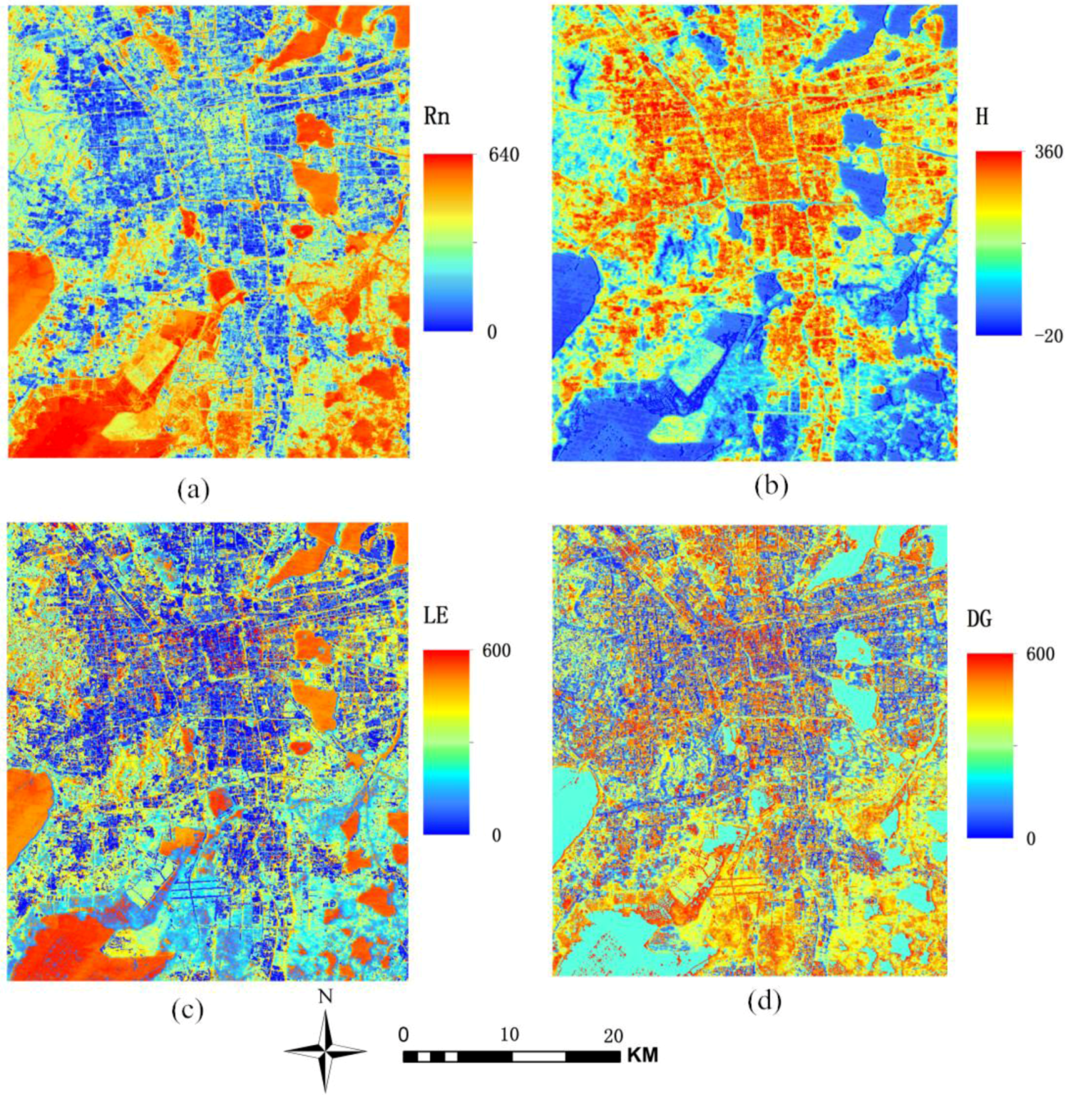
3.2. Spatial Pattern of Heat Energy
| Rn | H | LE | DG | LST | ||||||
|---|---|---|---|---|---|---|---|---|---|---|
| Mean | SD | Mean | SD | Mean | SD | Mean | SD | Mean | SD | |
| Water | 593.5 | 18.5 | −8.9 | 7.6 | 477.3 | 29.2 | 118.4 | 16.2 | 295.6 | 2.1 |
| Bare soil | 490.2 | 35.6 | 17.8 | 8.6 | 157.1 | 31.4 | 315.5 | 68.3 | 302.5 | 2.1 |
| Crop | 528.8 | 28.1 | 21.1 | 23.8 | 352.2 | 72.3 | 169.4 | 111.6 | 299.8 | 2.1 |
| Lawn | 474.3 | 17.3 | 10.9 | 5.8 | 282.8 | 19.8 | 190.6 | 361 | 300.8 | 1.5 |
| Forest | 534.2 | 19.2 | 13.2 | 19.5 | 462.6 | 46.9 | 59.4 | 73.6 | 298.8 | 1.2 |
| Low-medium density ISA | 491.5 | 24.2 | 90.4 | 36.7 | 207.9 | 85.7 | 214.1 | 95.8 | 302.6 | 1.8 |
| High density ISA | 485.7 | 46.4 | 104.9 | 40.2 | 47.8 | 72.7 | 334.0 | 106.5 | 303.3 | 2.0 |
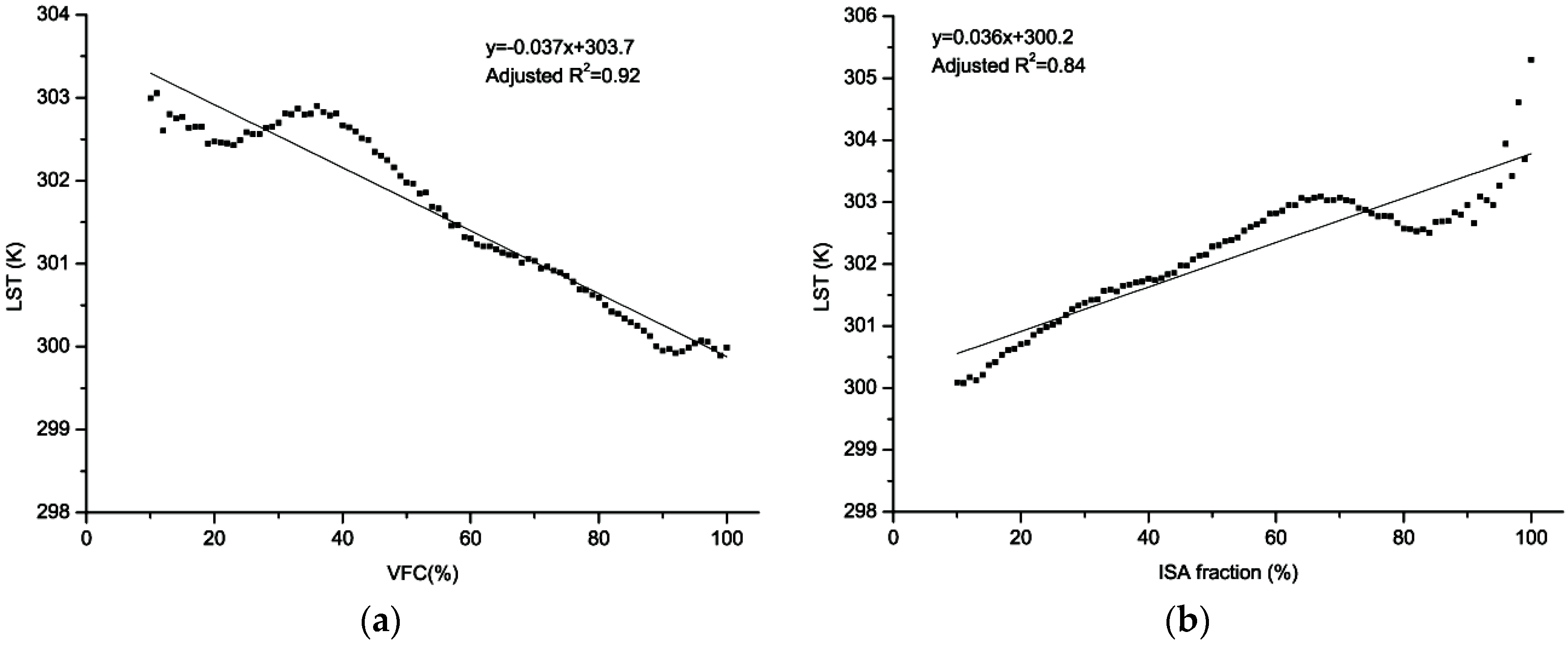
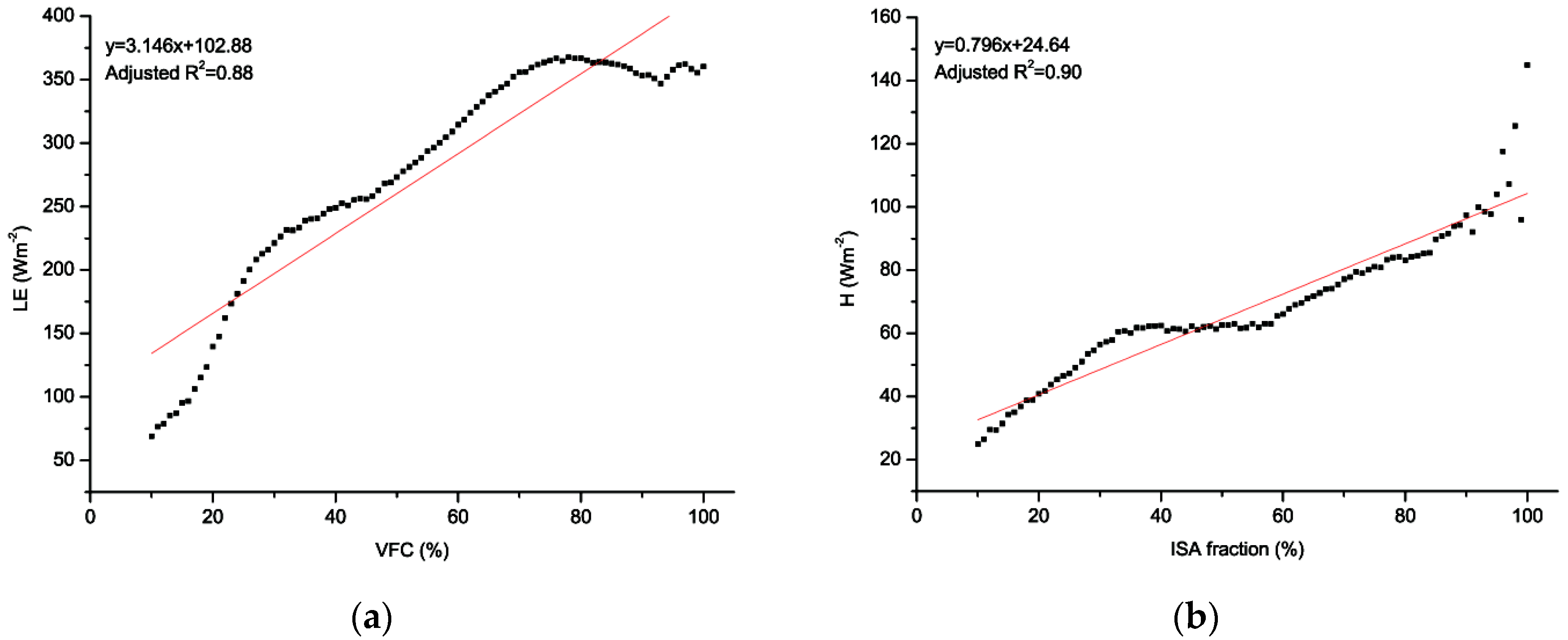
3.3. The Relationships between Heat Energy and VFC and ISA%
| LE | LST | |||
|---|---|---|---|---|
| VFC | Mean | SD | Mean | SD |
| <10% | 66.5 | 122.8 | 302.6 | 2.7 |
| 10%–30% | 174.2 | 122.1 | 302.6 | 2.1 |
| 30%–50% | 253.3 | 109.7 | 302.5 | 2.3 |
| 50%–70% | 325.3 | 98.6 | 301.3 | 2.3 |
| >70% | 361.3 | 81.7 | 299.9 | 2.1 |
| H | LST | |||
|---|---|---|---|---|
| ISA | Mean | SD | Mean | SD |
| <10% | 15.8 | 23.1 | 299.4 | 1.9 |
| 10%–30% | 44.2 | 40.1 | 300.9 | 2.3 |
| 30%–50% | 61.1 | 46.0 | 301.8 | 2.2 |
| 50%–70% | 68.0 | 49.6 | 302.8 | 2.1 |
| >70% | 88.1 | 48.9 | 303.0 | 2.2 |


3.4. Significance and Future Work
4. Conclusions
Acknowledgments
Author Contributions
Conflicts of Interest
References
- Phinn, S.; Stanford, M.; Scarth, P.; Murray, A.; Shyy, P. Monitoring the composition of urban environments based on the vegetation-impervious surface-soil (VIS) model by subpixel analysis techniques. Int. J. Remote Sens. 2002, 23, 4131–4153. [Google Scholar] [CrossRef]
- Raynolds, M.; Comiso, J.; Walker, D.; Verbyla, D. Relationship between satellite-derived land surface temperatures, arctic vegetation types, and NDVI. Remote Sens. Environ. 2008, 112, 1884–1894. [Google Scholar] [CrossRef]
- Weng, Q.; Lu, D.; Schubring, J. Estimation of land surface temperature-vegetation abundance relationship for urban heat island studies. Remote Sens. Environ. 2004, 89, 467–483. [Google Scholar] [CrossRef]
- Mackey, C.W.; Lee, X.; Smith, R.B. Remotely sensing the cooling effects of city scale efforts to reduce urban heat island. Build. Environ. 2012, 49, 348–358. [Google Scholar] [CrossRef]
- Holt, T.; Pullen, J. Urban canopy modeling of the new york city metropolitan area: A comparison and validation of single- and multilayer parameterizations. Mon. Weather Rev. 2007, 135, 1906–1930. [Google Scholar] [CrossRef]
- Oke, T.R. The energetic basis of the urban heat island. Quart. J. R. Meteorol. Soc. 1982, 108, 1–24. [Google Scholar] [CrossRef]
- Zhang, Y.; Odeh, I.O.; Han, C. Bi-temporal characterization of land surface temperature in relation to impervious surface area, NDVI and NDBI, using a sub-pixel image analysis. Int. J. Appl. Earth Obs. Geoinform. 2009, 11, 256–264. [Google Scholar] [CrossRef]
- Oke, T.; Spronken-Smith, R.; Jauregui, E.; Grimmond, C. The energy balance of central mexico city during the dry season. Atmos. Environ. 1999, 33, 3919–3930. [Google Scholar] [CrossRef]
- Quah, A.K.L.; Roth, M. Diurnal and weekly variation of anthropogenic heat emissions in a tropical city, singapore. Atmos. Environ. 2012, 46, 92–103. [Google Scholar] [CrossRef]
- Christen, A.; Vogt, R. Energy and radiation balance of a central european city. Int. J. Climatol. 2004, 24, 1395–1421. [Google Scholar] [CrossRef]
- Sham, J.F.C.; Memon, S.A.; Lo, Y.T. Application of continuous surface temperature monitoring technique for investigation of nocturnal sensible heat release characteristics by building fabrics in Hong Kong. Energy Build. 2013, 58, 1–10. [Google Scholar] [CrossRef]
- Mirzaei, P.A.; Haghighat, F. Approaches to study urban heat island—Abilities and limitations. Build. Environ. 2010, 45, 2192–2201. [Google Scholar] [CrossRef]
- Kato, S.; Yamaguchi, Y. Analysis of urban heat-island effect using aster and ETM+ data: Separation of anthropogenic heat discharge and natural heat radiation from sensible heat flux. Remote Sens. Environ. 2005, 99, 44–54. [Google Scholar] [CrossRef]
- Kato, S.; Liu, C.-C.; Sun, C.-Y.; Chen, P.-L.; Tsai, H.-Y.; Yamaguchi, Y. Comparison of surface heat balance in three cities in taiwan using Terra ASTER and formosat-2 RSI data. Int. J. Appl. Earth Obs. Geoinform. 2012, 18, 263–273. [Google Scholar] [CrossRef]
- Zhou, Y.; Weng, Q.; Gurney, K.R.; Shuai, Y.; Hu, X. Estimation of the relationship between remotely sensed anthropogenic heat discharge and building energy use. ISPRS J. Photogramm. Remote Sens. 2012, 67, 65–72. [Google Scholar] [CrossRef]
- Xu, W.; Wooster, M.J.; Grimmond, C.S.B. Modelling of urban sensible heat flux at multiple spatial scales: A demonstration using airborne hyperspectral imagery of Shanghai and a temperature-emissivity separation approach. Remote Sens. Environ. 2008, 112, 3493–3510. [Google Scholar] [CrossRef]
- Kato, S.; Yamaguchi, Y. Estimation of storage heat flux in an urban area using aster data. Remote Sens. Environ. 2007, 110, 1–17. [Google Scholar] [CrossRef]
- Kato, S.; Yamaguchi, Y.; Liu, C.-C.; Sun, C.-Y. Surface heat balance analysis of tainan city on March 6, 2001 using ASTER and formosat-2 data. Sensors 2008, 8, 6026–6044. [Google Scholar] [CrossRef]
- Yuan, F.; Bauer, M.E. Comparison of impervious surface area and normalized difference vegetation index as indicators of surface urban heat island effects in Landsat imagery. Remote Sens. Environ. 2007, 106, 375–386. [Google Scholar] [CrossRef]
- Weng, Q.; Lu, D.; Liang, B. Urban surface biophysical descriptors and land surface temperature variations. Photogrammetric Eng. Remote Sens. 2006, 72, 1275–1286. [Google Scholar] [CrossRef]
- Rashed, T.; Weeks, J.R.; Gadalla, M.S.; Hill, A.G. Revealing the anatomy of cities through spectral mixture analysis of multispectral satellite imagery: A case study of the Greater Cairo Region, Egypt. Geocarto Int. 2001, 16, 7–18. [Google Scholar] [CrossRef]
- Weng, Q.; Lu, D. A sub-pixel analysis of urbanization effect on land surface temperature and its interplay with impervious surface and vegetation coverage in Indianapolis, United States. Int. J. Appl. Earth Obs. Geoinform. 2008, 10, 68–83. [Google Scholar] [CrossRef]
- Ridd, M.K. Exploring a V-I-S (vegetation-impervious surface-soil) model for urban ecosystem analysis through remote sensing: Comparative anatomy for cities. Int. J. Remote Sens. 1995, 16, 2165–2185. [Google Scholar] [CrossRef]
- Gluch, R.; Quattrochi, D.A.; Luvall, J.C. A multi-scale approach to urban thermal analysis. Remote Sens. Environ. 2006, 104, 123–132. [Google Scholar] [CrossRef]
- Gillies, R.R.; Brim Box, J.; Symanzik, J.; Rodemaker, E.J. Effects of urbanization on the aquatic fauna of the Line Creek watershed, Atlanta—A satellite perspective. Remote Sens. Environ. 2003, 86, 411–422. [Google Scholar] [CrossRef]
- Mallick, J.; Rahman, A.; Singh, C.K. Modeling urban heat islands in heterogeneous land surface and its correlation with impervious surface area by using night-time aster satellite data in highly urbanizing city, Delhi-India. Adv. Space Res. 2013, 52, 639–655. [Google Scholar] [CrossRef]
- Roberts, D.A.; Gardner, M.; Church, R.; Ustin, S.; Scheer, G.; Green, R. Mapping chaparral in the Santa Monica Mountains using multiple endmember spectral mixture models. Remote Sens. Environ. 1998, 65, 267–279. [Google Scholar] [CrossRef]
- Yang, J.; He, Y.; Oguchi, T. An endmember optimization approach for linear spectral unmixing of fine-scale urban imagery. Int. J. Appl. Earth Obs. Geoinform. 2014, 27, 137–146. [Google Scholar] [CrossRef]
- Feizizadeh, B.; Blaschke, T. Examining urban heat island relations to land use and air pollution: Multiple endmember spectral mixture analysis for thermal remote sensing. IEEE J. Sel. Top. Appl. Earth Obs. Remote Sens. 2013, 6, 1749–1756. [Google Scholar] [CrossRef]
- Zhang, N.; Gao, Z.; Wang, X.; Chen, Y. Modeling the impact of urbanization on the local and regional climate in Yangtze River Delta, China. Theor. Appl. Climatol. 2010, 102, 331–342. [Google Scholar] [CrossRef]
- Zhang, N.; Zhu, L.; Zhu, Y. Urban heat island and boundary layer structures under hot weather synoptic conditions: A case study of Suzhou City, China. Adv. Atmos. Sci. 2011, 28, 855–865. [Google Scholar] [CrossRef]
- Cooley, T.; Anderson, G.; Felde, G.; Hoke, M.; Ratkowski, A.; Chetwynd, J.; Gardner, J.; Adler-Golden, S.; Matthew, M.; Berk, A. Flaash, a Modtran4-based atmospheric correction algorithm, its application and validation. In Proceedings of the 2002 IEEE International Geoscience and Remote Sensing Symposium, Toronto, ON, Canada, 24–28 June 2002; pp. 1414–1418.
- Jiménez-Muñoz, J.C.; Sobrino, J.A. A generalized single-channel method for retrieving land surface temperature from remote sensing data. J. Geophys. Res. Atmos. (1984–2012) 2003, 108. [Google Scholar] [CrossRef]
- Sobrino, J.; Raissouni, N.; Li, Z.-L. A comparative study of land surface emissivity retrieval from NOAA data. Remote Sens. Environ. 2001, 75, 256–266. [Google Scholar] [CrossRef]
- Sobrino, J.A.; Jiménez-Muñoz, J.C.; Paolini, L. Land surface temperature retrieval from Landsat TM 5. Remote Sens. Environ. 2004, 90, 434–440. [Google Scholar] [CrossRef]
- Jiménez-Muñoz, J.C.; Sobrino, J.A.; Gillespie, A.; Sabol, D.; Gustafson, W.T. Improved land surface emissivities over agricultural areas using ASTER NDVI. Remote Sens. Environ. 2006, 103, 474–487. [Google Scholar] [CrossRef]
- Nunez, M.; Oke, T.R. Energy balance of an urban canyon. J. Appl. Meteor. 1977, 16, 11–19. [Google Scholar] [CrossRef]
- Liang, S. Narrowband to broadband conversions of land surface albedo I: Algorithms. Remote Sens. Environ. 2001, 76, 213–238. [Google Scholar] [CrossRef]
- Brutsaert, W. Evaporation into the Atmosphere: Theory, History and Applications (Environmental Fluid Mechanics); Springer: Houten, The Netherland, 1982; p. 302. [Google Scholar]
- Allen, R.G.; Pereira, L.S.; Raes, D.; Smith, M. Crop Evapotranspiration—Guidelines for Computing Crop Water Requirements—FAO Irrigation and Drainage Paper 56; FAO Technical Papers; Food and Agriculture Organization: Rome, Italy, 1998; p. 6541. [Google Scholar]
- Wong, M.S.; Yang, J.; Nichol, J.; Weng, Q.; Menenti, M.; Chan, P.W. Modeling of anthropogenic heat flux using HJ-1B Chinese small satellite image: A study of heterogeneous urbanized areas in Hong Kong. IEEE Geosci. Remote Sens. Lett. 2015, 12, 1466–1470. [Google Scholar] [CrossRef]
- Grimmond, C. Aerodynamic roughness of urban areas derived from wind observations. Bound. Layer Meteorol. 1998, 89, 1–24. [Google Scholar] [CrossRef]
- Moriwaki, R.; Kanda, M. Scalar roughness parameters for a suburban area. J. Meteorol. Soc. Jpn. 2006, 84, 1063–1071. [Google Scholar] [CrossRef]
- Stewart, J.B.; Kustas, W.P.; Humes, K.S.; Nichols, W.D.; Moran, M.S.; De Bruin, H. Sensible heat flux-radiometric surface temperature relationship for eight semiarid areas. J. Appl. Meteorol. 1994, 33, 1110–1117. [Google Scholar] [CrossRef]
- Weng, Q.; Hu, X.; Quattrochi, D.; Liu, H. Assessing intra-urban surface energy fluxes using remotely sensed aster imagery and routine meteorological data: A case study in Indianapolis, USA. IEEE J. Sel. Top. Appl. Earth Obs. Remote Sens. 2014, 7, 4046–4057. [Google Scholar] [CrossRef]
- Suckling, P.W. The energy balance microclimate of a suburban lawn. J. Appl. Meteorol. 1980, 19, 606–608. [Google Scholar] [CrossRef]
- Jarvis, P. The interpretation of the variations in leaf water potential and stomatal conductance found in canopies in the field. Philos. Trans. R. Soc. Lond. B Biol. Sci. 1976, 273, 593–610. [Google Scholar] [CrossRef]
- Nishida, K.; Nemani, R.R.; Running, S.W.; Glassy, J.M. An operational remote sensing algorithm of land surface evaporation. J. Geophys. Res. Atmos. (1984–2012) 2003, 108. [Google Scholar] [CrossRef]
- Kelliher, F.; Leuning, R.; Raupach, M.; Schulze, E.-D. Maximum conductances for evaporation from global vegetation types. Agric. For. Meteorol. 1995, 73, 1–16. [Google Scholar] [CrossRef]
- Boardman, J.W.; Kruse, F.A.; Green, R.O. Mapping target signatures via partial unmixing of AVIRIS data. In Proceedings of the 5th Annual JPL Airborne Earth Science Workshop, Pasadena, CA, USA, 23–26 January 1995; pp. 23–26.
- Roberts, D.A.; Gardner, M.E.; Church, R.; Ustin, S.L.; Green, R.O. Optimum strategies for mapping vegetation using multiple-endmember spectral mixture models. Proc. SPIE 1997. [Google Scholar] [CrossRef]
- Dennison, P.E.; Roberts, D.A. Endmember selection for multiple endmember spectral mixture analysis using endmember average RMSE. Remote Sens. Environ. 2003, 87, 123–135. [Google Scholar] [CrossRef]
- Roberts, D.; Halligan, K.; Dennison, P. Viper Tools User Manual (Version 1.5); University of California: Santa Barbara, CA, USA, 2007. [Google Scholar]
- Liu, K.; Su, H.; Zhang, L.; Yang, H.; Zhang, R.; Li, X. Analysis of the urban heat island effect in Shijiazhuang, China using satellite and airborne data. Remote Sens. 2015, 7, 4804–4833. [Google Scholar] [CrossRef]
- Liu, K.; Su, H.; Li, X. Estimating high-resolution urban surface temperature using a hyperspectral thermal mixing (HTM) approach. IEEE J. Sel. Top. Appl. Earth Obs. Remote Sens. 2015. [Google Scholar] [CrossRef]
- Ju, W.; Gao, P.; Wang, J.; Zhou, Y.; Zhang, X. Combining an ecological model with remote sensing and GIS techniques to monitor soil water content of croplands with a monsoon climate. Agric. Water Manag. 2010, 97, 1221–1231. [Google Scholar] [CrossRef]
- Gao, Z.; Liu, C.; Gao, W.; Chang, N.-B. A coupled remote sensing and the surface energy balance with Topography Algorithm (SEBTA) to estimate actual evapotranspiration over heterogeneous terrain. Hydrol. Earth Syst. Sci. 2011, 15, 119–139. [Google Scholar] [CrossRef] [Green Version]
- Liu, Y. Characteristics of Surface Heat Flux on Urban Island Effects Using Thermal Infrared Remote Sensing in China’s Typical City. Ph.D. Thesis, Graduate University of Chinese Academy of Sciences, Beijing, China, 2012. [Google Scholar]
- Unger, J.; Savić, S.; Gál, T. Modelling of the annual mean urban heat island pattern for planning of representative urban climate station network. Adv. Meteorol. 2011, 2011. [Google Scholar] [CrossRef]
- Zhou, W.; Huang, G.; Cadenasso, M.L. Does spatial configuration matter? Understanding the effects of land cover pattern on land surface temperature in urban landscapes. Landsc. Urban Plan. 2011, 102, 54–63. [Google Scholar] [CrossRef]
- Wu, H.; Ye, L.-P.; Shi, W.-Z.; Clarke, K.C. Assessing the effects of land use spatial structure on urban heat islands using HJ-1B remote sensing imagery in Wuhan, China. Int. J. Appl. Earth Obs. Geoinform. 2014, 32, 67–78. [Google Scholar] [CrossRef]
- Grimmond, C.; Oke, T.R. Comparison of heat fluxes from summertime observations in the suburbs of four north American cities. 1995, 34, 873–889. [Google Scholar]
- Gao, Z.; Gao, W.; Chang, N.-B. Evaluation of dynamic linkages between evapotranspiration and land-use/land-cover changes with Landsat TM and ETM+ data. Int. J. Remote Sens. 2012, 33, 3733–3750. [Google Scholar] [CrossRef]
- Chen, X.-L.; Zhao, H.-M.; Li, P.-X.; Yin, Z.-Y. Remote sensing image-based analysis of the relationship between urban heat island and land use/cover changes. Remote Sens. Environ. 2006, 104, 133–146. [Google Scholar] [CrossRef]
- Shashua-Bar, L.; Pearlmutter, D.; Erell, E. The cooling efficiency of urban landscape strategies in a hot dry climate. Landsc. Urban Plan. 2009, 92, 179–186. [Google Scholar] [CrossRef]
- Cohen, P.; Potchter, O.; Matzarakis, A. Daily and seasonal climatic conditions of green urban open spaces in the mediterranean climate and their impact on human comfort. Build. Environ. 2012, 51, 285–295. [Google Scholar] [CrossRef]
- Grimmond, C.; Souch, C.; Hubble, M. Influence of tree cover on summer-time surface energy balance fluxes, San Gabriel Valley, Los Angeles. Clim. Res. 1996, 6, 45–57. [Google Scholar] [CrossRef]
- Oke, T. Advectively-assisted evapotranspiration from irrigated urban vegetation. Bound. Layer Meteorol. 1979, 17, 167–173. [Google Scholar] [CrossRef]
- Kuang, W.; Dou, Y.; Zhang, C.; Chi, W.; Liu, A.; Liu, Y.; Zhang, R.; Liu, J. Quantifying the heat flux regulation of metropolitan land use/land cover components by coupling remote sensing modeling with in situ measurement. J. Geophys. Res. Atmos. 2015. [Google Scholar] [CrossRef]
- Zhang, Y.; Balzter, H.; Wu, X. Spatial-temporal patterns of urban anthropogenic heat discharge in Fuzhou, China, observed from sensible heat flux using Landsat TM/ETM+ data. Int. J. Remote Sens. 2013, 34, 1459–1477. [Google Scholar] [CrossRef]
- Boegh, E.; Poulsen, R.N.; Butts, M.; Abrahamsen, P.; Dellwik, E.; Hansen, S.; Hasager, C.B.; Ibrom, A.; Loerup, J.K.; Pilegaard, K.; et al. Remote sensing based evapotranspiration and runoff modeling of agricultural, forest and urban flux sites in Denmark: From field to macro-scale. J. Hydrol. 2009, 377, 300–316. [Google Scholar] [CrossRef]
- Fernández-Manso, A.; Quintano, C.; Roberts, D. Evaluation of potential of multiple endmember spectral mixture analysis (MESMA) for surface coal mining affected area mapping in different world forest ecosystems. Remote Sens. Environ. 2012, 127, 181–193. [Google Scholar] [CrossRef]
- Tompkins, S.; Mustard, J.F.; Pieters, C.M.; Forsyth, D.W. Optimization of endmembers for spectral mixture analysis. Remote Sens. Environ. 1997, 59, 472–489. [Google Scholar] [CrossRef]
- Franke, J.; Roberts, D.A.; Halligan, K.; Menz, G. Hierarchical multiple endmember spectral mixture analysis (MESMA) of hyperspectral imagery for urban environments. Remote Sens. Environ. 2009, 113, 1712–1723. [Google Scholar] [CrossRef]
- Quintano, C.; Fernández-Manso, A.; Roberts, D.A. Multiple endmember spectral mixture analysis (MESMA) to map burn severity levels from landsat images in mediterranean countries. Remote Sens. Environ. 2013, 136, 76–88. [Google Scholar] [CrossRef]
© 2016 by the authors; licensee MDPI, Basel, Switzerland. This article is an open access article distributed under the terms and conditions of the Creative Commons by Attribution (CC-BY) license (http://creativecommons.org/licenses/by/4.0/).
Share and Cite
Liu, K.; Fang, J.-y.; Zhao, D.; Liu, X.; Zhang, X.-h.; Wang, X.; Li, X.-k. An Assessment of Urban Surface Energy Fluxes Using a Sub-Pixel Remote Sensing Analysis: A Case Study in Suzhou, China. ISPRS Int. J. Geo-Inf. 2016, 5, 11. https://0-doi-org.brum.beds.ac.uk/10.3390/ijgi5020011
Liu K, Fang J-y, Zhao D, Liu X, Zhang X-h, Wang X, Li X-k. An Assessment of Urban Surface Energy Fluxes Using a Sub-Pixel Remote Sensing Analysis: A Case Study in Suzhou, China. ISPRS International Journal of Geo-Information. 2016; 5(2):11. https://0-doi-org.brum.beds.ac.uk/10.3390/ijgi5020011
Chicago/Turabian StyleLiu, Kai, Jun-yong Fang, Dong Zhao, Xue Liu, Xiao-hong Zhang, Xiao Wang, and Xue-ke Li. 2016. "An Assessment of Urban Surface Energy Fluxes Using a Sub-Pixel Remote Sensing Analysis: A Case Study in Suzhou, China" ISPRS International Journal of Geo-Information 5, no. 2: 11. https://0-doi-org.brum.beds.ac.uk/10.3390/ijgi5020011