Time-Series and Frequency-Spectrum Correlation Analysis of Bridge Performance Based on a Real-Time Strain Monitoring System

Abstract

Monitoring bridges’ performance is a vital task to ensure their safety and to plan their maintenance operations. Therefore, it is very important to monitor bridges’ behavior and to analyze their measured data. In this study, the time-series and frequency-spectrum correlation analyses are used to study the performance of Fu-Sui Bridge under harsh environmental and traffic loads. It investigates the bridge performance based on a real-time strain monitoring system, and the ambient environmental and traffic loads are studied and discussed. Furthermore, a simplified method based on signal processing is developed and used to estimate the traffic volumes. The results of this study reveal that the traffic loads influence on static strain is obviously lower than that of air temperature and temperature changes of the bridge cross-section; the non-linearity behavior of the bridge during summer time is more than winter time; and the stability of the whole bridge during winter time is more than during summer time. The time-series and vibration analyses also show that the bridge performance in terms of its rigidity and stability is higher during winter time.

1. Introduction

To estimate the performance of structures, recently, structural health monitoring (SHM) systems have been developed and enhanced using advanced measurement sensors and monitoring networks [1,2]. SHM is used to detect the displacements and damage of civil engineering infrastructures based on the changes of their physical properties, such as mass and stiffness [3,4]. The fundamental structures changes can be estimated based on structure parameter changes, like resonance frequencies, mode shapes and modal damping. The structures’ parameters are affected by the varying operational and environmental conditions [4]. In SHM systems, two types of sensors are utilized to collect structure data; the first type is used to collect the input data (environmental, traffic, etc.), and the second type is to collect the behavior of the structure (displacement, acceleration, strain, etc.). Sohn et al. [3] provided a literature review of SHM, vibration analysis and damage detection. Furthermore, Follen et al. [5] presented a previous SHM literature review and its use to identify bridges’ performance.

Strain measurements are widely used to study the safety of structures, because they provide rich information about the stresses experienced by the structures during their operation [1,6,7]. Real-time monitoring systems, or long-term continuous monitoring, of dynamic strain are critical in the assessment, inspection and decision making of bridges and other engineering structures’ maintenance [7,8]. For example, Follen et al. [5] counted the truck events based on strain measurements. Therefore, strain measurements can be used to assess bridges performance under combined loads’ effects. The strain measurements contain static and dynamic strains and noises measurements. The static strain performance is due to the combined effect of both the temperature and traffic loads [8,9]. Furthermore, Wang et al. [9] concluded that the daily or seasonal temperature field causes critical strain levels, even higher than traffic-induced strains. Therefore, abnormal variation of the correlation between the temperature field and its static strain effect can indicate static performance degradation of bridge structures. Miao et al. [4] stated that the temperature condition is a common important parameter in structures’ condition assessment. The dynamic strain, on the other hand, refers to the peaks or impulse strain measurements that can be used to estimate the traffic volume passing on the bridge. Furthermore, the covered noises of measurements should be removed first by applying a filter process. In this study, a temperature and strain SHM system is used to analyze the performance of the Fu-Sui Bridge, China. As such, the study focuses on strain measurements to assess the Fu-Sui Bridge and counts the traffic volume based on a simple developed method.

The time-series correlation analysis is one of the methods used widely in analyzing and classifying data in SHM systems. Omenzetter and Brownjohn [10] applied the autoregressive integrated moving average (ARIMA) model for the recorded strain signals and analyzed bridge performance based on observing the changes in the ARIMA coefficients and correlation analysis of ARIMA parameters. Liu et al. [6] studied the correlation among bridge components’ safety under actual traffic and strain data. They also represented the sensitivity of measurements of strain based on system modeling, correlations, probability distribution, measurement errors and number of observations. Follen et al. [5] used the correlation analysis of the probability density function to estimate the behavior of bridges and to study the damage detection based on strain measurements. Wang et al. [9] applied the correlation of the multivariate linear regression modeling, principal component analysis and residual strain analysis to study the performance of steel bridges due to temperature variation effects. Hu and Kaloop [11] studied the performance of bridges during harsh environmental effects based on the changes of the correlation of the model identification parameters with input-output wavelet model identification.

The frequency domain analysis is used to detect the dynamic performance of structures [12,13]. Hong et al. [12] introduced the application of the time frequency and power spectrum density of strain simulation to estimate the failure of materials. Wu et al. [14] studied the dynamic performance of bridges based on strain measurements, and they found that the noise is affecting the frequency modes’ calculation. Furthermore, they found that low frequency modes occurred due to temperature variation. Mata et al. [15] studied the dynamic performance of a concrete dam using time-frequency correlation analysis of the displacement sensor and air temperature changes. In their study, they concluded that this method can be used for continuous assessment of the performance and safety of the dam. The dynamic property changes of bridges are studied based on air temperature changes in Xia et al. [16]. Xia et al. [16] showed that the fundamental frequency of bridges is in high negative correlation with the air temperature, while the damping ratio is in positive correlation with temperature for the fundamental frequency mode.

The time-series and frequency-spectrum are applied in this study on the data collected for both the real-time strains and the temperature changes. In addition, a novel application of signal processing is used to estimate the traffic volume based on strain measurements. Simplified model identification is used to classify the affected loads on the strain measurements, and the static strain performance of the bridge is studied under harsh environmental effects. Furthermore, the power spectrum density of real strain measurements is presented and discussed.

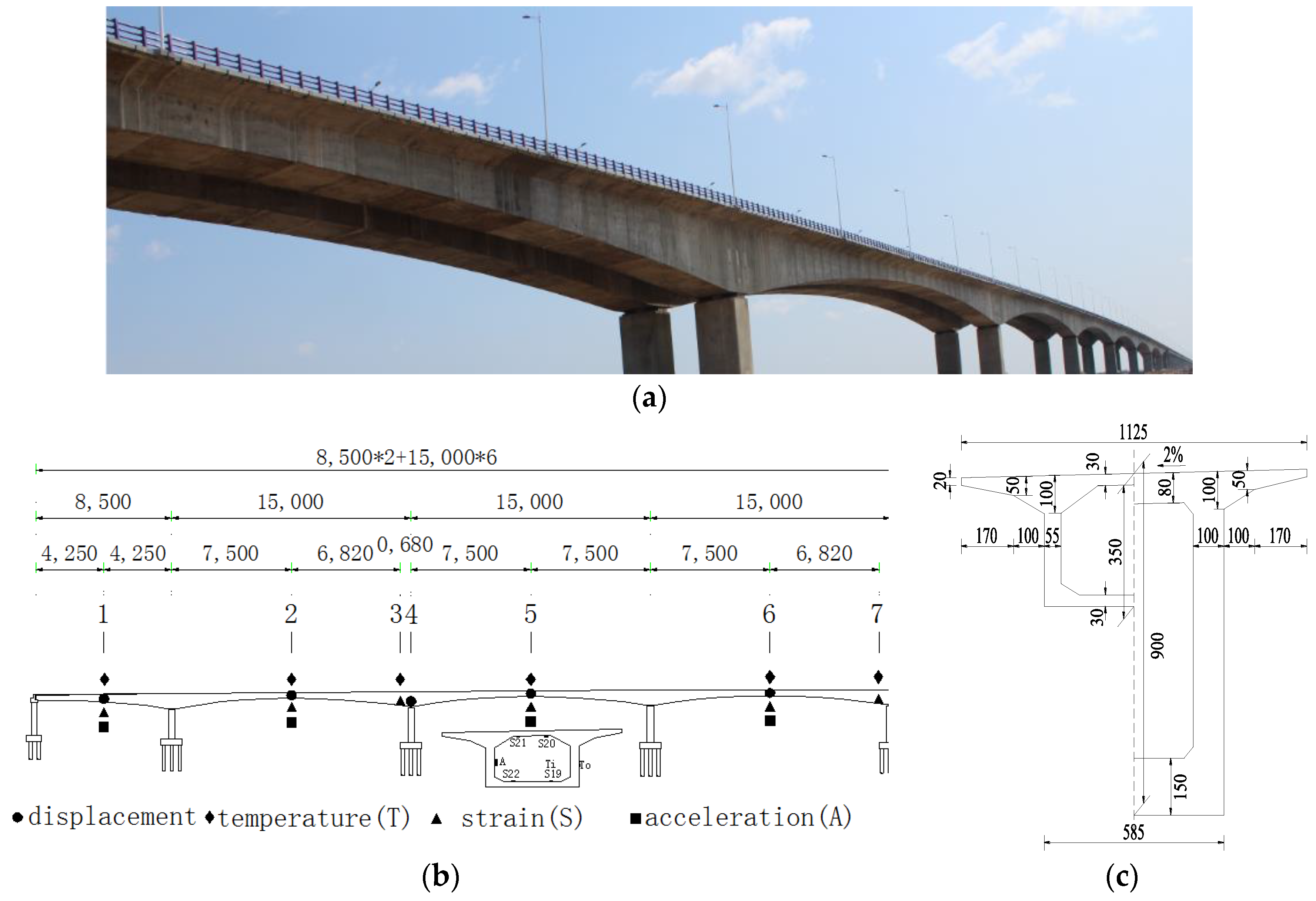
2. Fu-Sui Bridge and SHM System

The monitoring object of this research is the Fu-Sui Bridge, which is designed to cross the Songhua River and connect the Fu-Sui high speed highway with a total length of 1170 m. The bridge deck is formed of a main continuous prestressed concrete box-girder. The bridge consists of eight continuous spans; two outer spans, 80 m each, and six inner spans, 150 m each (Figure 1). The main girder of the bridge is made of segments cast in place with post-tensioned steel. As shown in Figure 1c, the cross-section of the main girder is a single cell box, with its height varying from 9 m (pier section) to 3.5 m (mid-span section), including a top slab of 11.25 m in width, a bottom slab of 5.85 m in width and a 2.7-m length of web slab on each side. The weather at the bridge site area is extremely cold in the winter with no outdoor work being possible during November to the following April.

The monitoring system was designed just after the opening of the bridge for traffic, and the installation was conducted in mid-April 2012. In order to record the temperature variations of the concrete of the box-girder regularly, 24 FBG strain (S) sensors are installed in six positions (four sensors at each position) in the top and bottom inside of the box-girder plates, as shown in Figure 1b. The strain (Si) denotes the i-th strain sensor number (where i = 1, 2, …, 24) to continuously obtain axial static strain data. Furthermore, one FBG temperature (T) sensor is installed at each of these (i) sections; while six temperature sensors are installed inside and outside Section Number “3”, as shown in Figure 1b. The (Ti) denotes the i-th number of the temperature sensor (where i = 1, 2, …, 12) to continuously measure temperature field data. Since the changes of temperature and strain are very high and fast, the sampling frequency of data collection is set to an appropriate value of 25 Hz. In addition, four uniaxial acceleration sensors are installed in the four mid-spans of the bridge to acquire the dynamic data and ten hydrostatic leveling subsystems (HLS) to measure static displacement. More detail about the monitoring system and previous studies can be found in [11,17,18].

In this paper, the bridge performance is studied at Cross-section 5, where full monitoring data are available. At this section, four monitoring strain points, S19, S20, S21 and S22, two monitoring temperature points, Ti (inside) and To (outside), and one accelerometer point (A) are installed, as shown in Figure 1b. The study is performed over four selected months to estimate the effect of temperature changes on the section performance. The maximum variation of temperature changes occurred in May 2012 and March 2013, while the maximum and minimum observed ambient temperature occurred in May 2012 and January 2013 [11]. Figure 2 presents the maximum and minimum observed temperature on the bridge site during one year. The maximum and minimum temperature changes are noted during May and June 2012 and January 2013, respectively. The maximum variation between inside and outside the bridge box girder occurred during May 2012 (12.27 °C) and March 2013 (10.15 °C). Furthermore, the low positive and negative were in October 2012 (7.42 °C) and January 2013 (−21.92 °C), respectively. In addition, the maximum and minimum temperatures recorded were 30.25 °C and −21.92 °C. However, to study the full performance of the bridge with the ambient and variation changes of temperature on the bridge deck, the following months are chosen: (1) May and October 2012 (the period of high temperature changes during the monitoring time), assuming that as summer time; (2) January and March 2013 (period of low temperature changes during the monitoring time), assuming that as winter time.

3. Data Measurements and Preprocessing

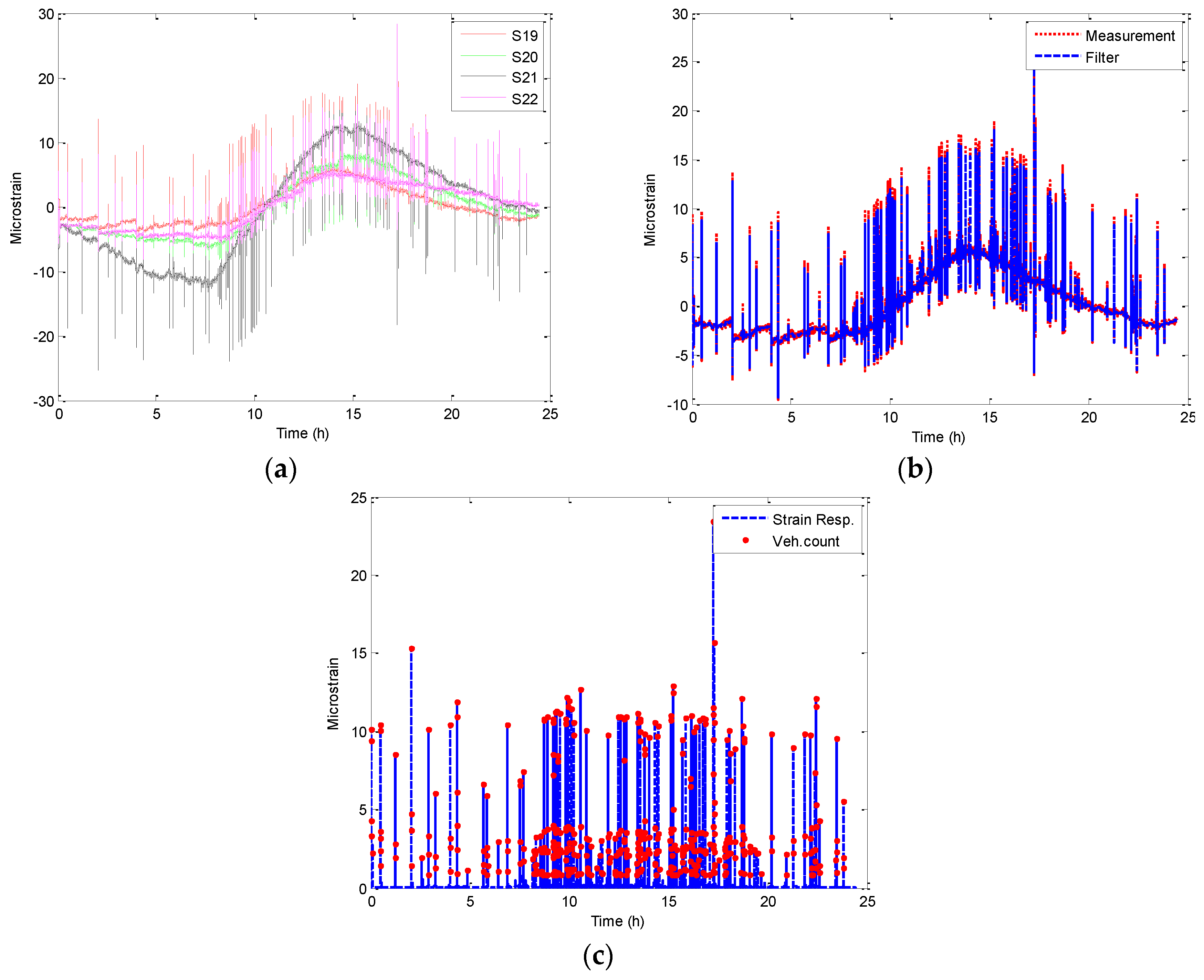
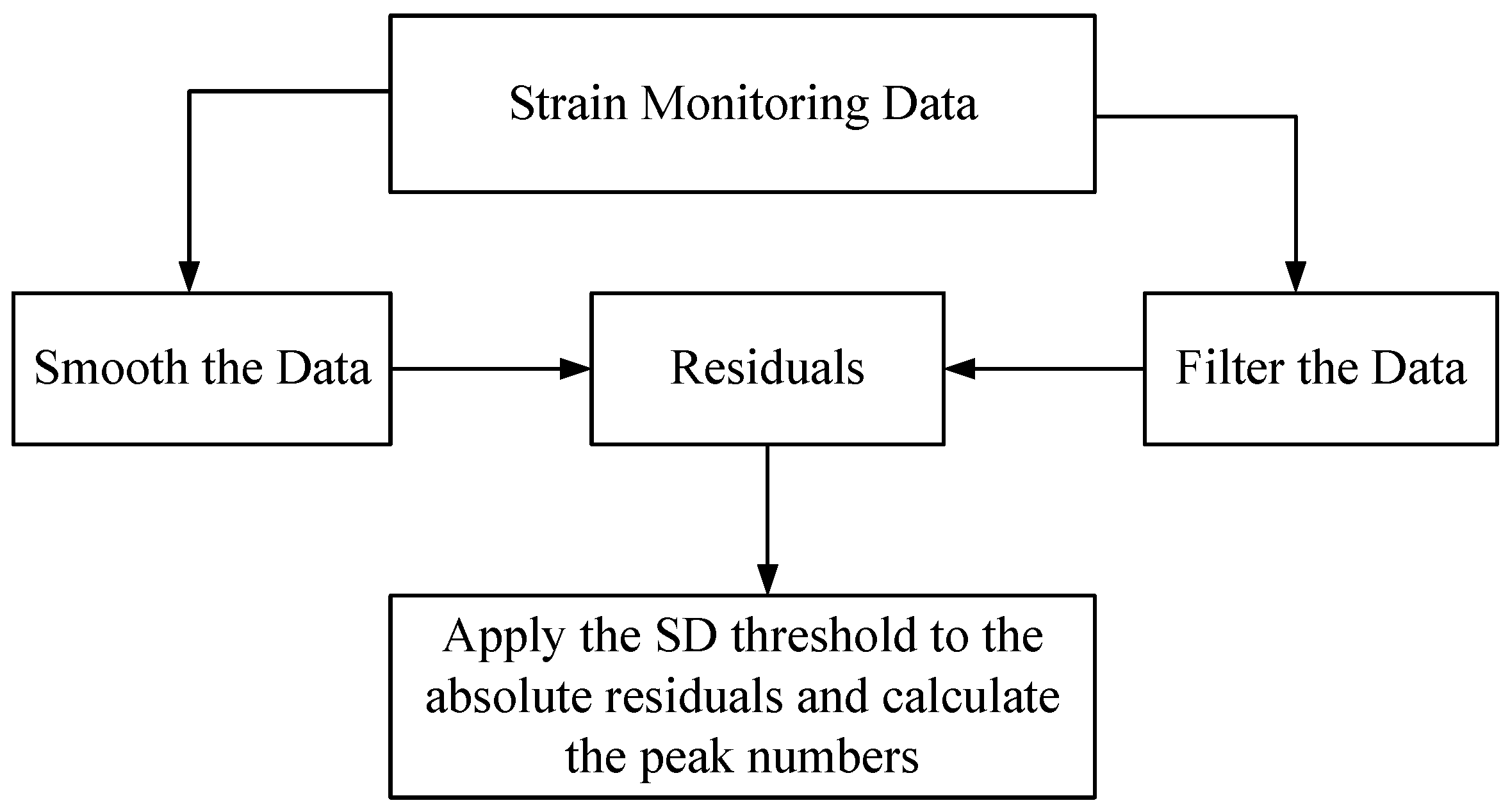
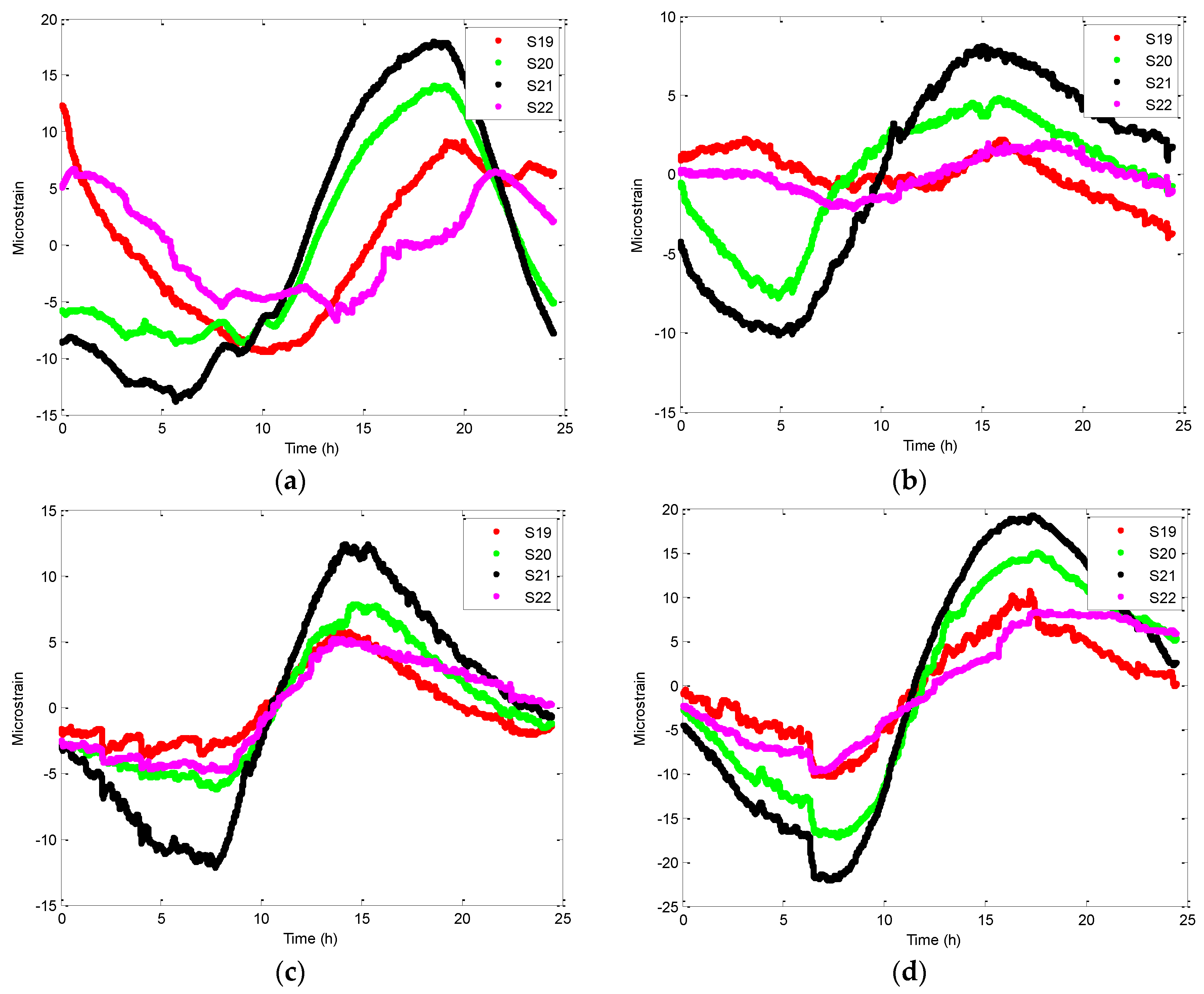
3.1. Temperature and Strain Preprocessing

The strain S19 and outside temperature for 21 May 2012 measurements are shown in Figure 3. From the previous studies conclusions [4,5,19], it has been stated that the strain measurements clearly show that the peak impulses are caused by traffic loads. Therefore, to estimate the temperature and strain changes, the traffic effects and noises should be first removed. Furthermore, each peak point corresponds to the time when traffic crosses the bridge [5,19], whereas the static strain shows a high response with temperature changes, as shown in Figure 3. The measurements of the strain and temperature data are refined and smoothed by eliminating the traffic and noise effects using the moving average (MA) filter. Based on the results of numerous trials of the MA filter steps, it is found that a simple low-pass MA filter with approximately a 1-s step allows us to separate measurements into static and dynamic components. The smoothed data (static component) are shown in Figure 3. It shows a high correlation and no information losses for the temperature and static strain measurements.

From Figure 3, it can be seen that the air temperature and strain measurements approximately have a similar trend. Furthermore, the performance of the strain follows a sine curve with approximately the same trend as the temperature changes. Thus, the temperature effect is a main factor of strain performance. Figure 4 shows the daily smoothed temperature monitoring data inside and outside the studied section for May 2012, October 2012, January 2013 and March 2013.

As shown in Figure 4, the smoothed temperature inside the section is approximately constant during the whole study period, while the maximum air temperature change varies between +15 and +5 °C for May and October 2012, respectively, and −7 and −10 °C for January and March 2013, respectively. Therefore, the air temperature and temperature changes of the section are the most influential factors of static strain variation based on the correlation between strain response and temperature effects, as shown in Figure 3.

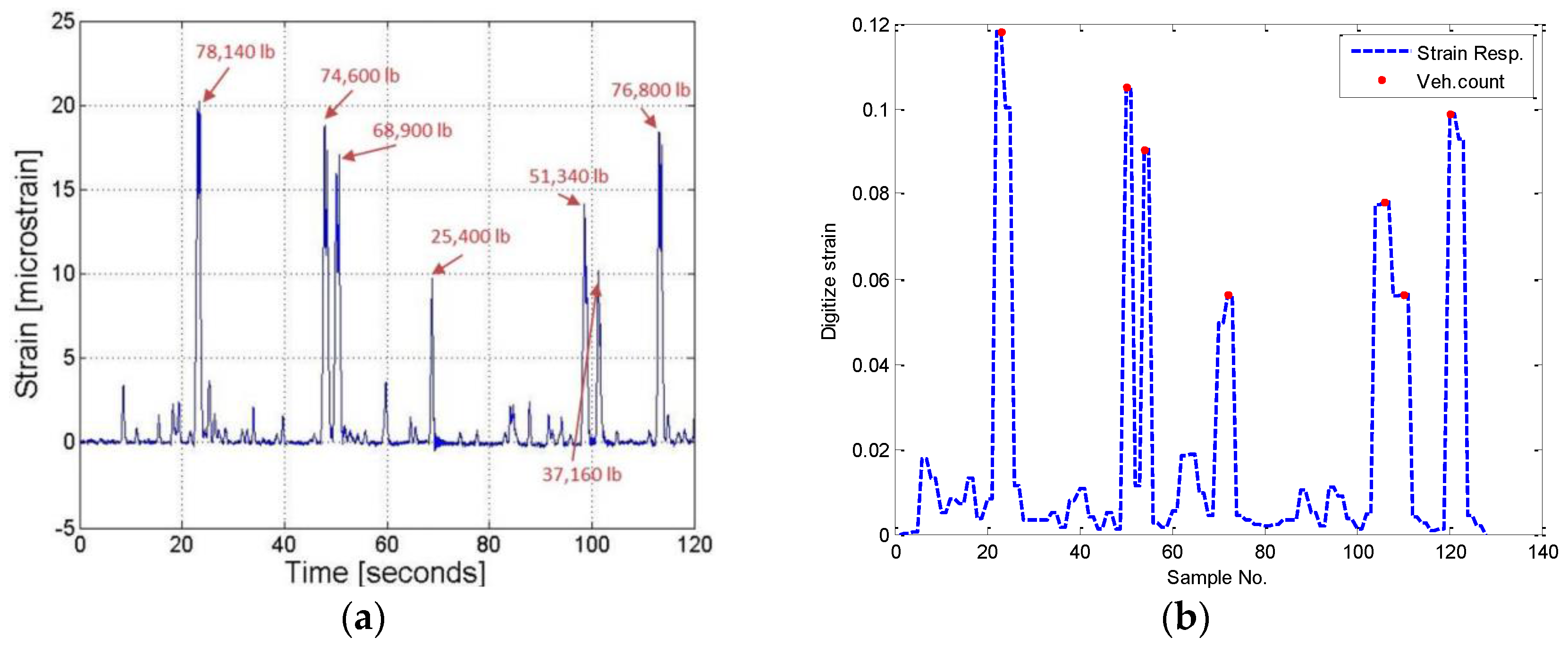
3.2. Traffic Strain Counter

The accuracy of the strain measurement used is high and the measurement ranges from −1500 to +1500 microstrain; more details about the sensors used can be found in Chen et al. [17]. Figure 5a shows the strains measurements in January 2013. It shows that the sensitivity of the upper and lower strains is high and occurred at the same time due to traffic effects. In order to measure the volume of the traffic crossing the bridge, the strain measurements used previously by [4,5] are adopted. The Follen method [5] counted the heavy truck events that are triggered above a given threshold (outlier) of recorded strains. It also works only when there is small noise affecting the strain measurements. In addition, Miao et al. [4] presented complex and parametric methods to count the traffic events, and their method needs a manual parameter selection. Therefore, the current development depends on the accuracy of strain measurements, and it is a simplified and non-parametric method, with a calculated threshold. Accordingly, the data should be filtered to remove measurement noises. The thresholds used in this case depend on the noise ratio. The original data are smoothed to increase the strain accuracy and enable calculating the traffic volume with small threshold values. The steps of the developed method for calculating the traffic volumes are: first, the measurements are filtered to estimate the accurate strain performance under traffic loads. For that purpose, wavelet decomposition is used to filter the strain measurements; more detail about this filter can be found in [1,9,20]. The wavelet decomposition Level 12 with wavelet mother db10 “Daubechies wavelets order 10” and an adaptive threshold are applied in this study (Figure 5b); second, the measurements are smoothed to estimate the static performance; third, the residuals between the filtered and smoothed data contain the impulse response of the traffic loads without or with little noise effect. Finally, the number of impulses of the absolute residuals are calculated with applied small threshold (the standard deviation, SD, of residuals is applied in this study) to eliminate the remaining smallest noises to reveal the amount of traffic. In addition, to classify the traffic types, different thresholds are used with two measurements, which are strain and video measurements.

To verify the developed traffic counting method, the data presented in Kolev [19] is used for comparison purposes. In his study, two minutes of strain sensor measurements are collected with seven trucks passing the bridge (Figure 6a). The digitizing method [21] is utilized to estimate the strain variation, and the developed signal processing method is used to detect the vehicles numbers (Figure 6b). The applied method shows that the seven trucks are counted as shown in Figure 6b, thus verifying the reliability of the developed method in counting the number of vehicles passing the bridge.

In this study, the developed method is also verified based on the vehicle number measured from the two strains, as shown in Figure 5. The vehicle numbers based on the two strain sensors S19 and S22 are equal. For a full-scale implementation of this method, more experimental work or field observation with video measurements can be done. Moreover, the thresholds values are changed based on the strain instruments’ accuracy. Figure 7 shows a simplified flowchart of the traffic counter design, and Figure 5c shows the traffic volume in January 2013 using S19 strain measurements.

In this study, the standard deviation of strain residuals is used as a threshold to eliminate the remaining noises [4]. The calculated traffic volume shows that the number of vehicles crossing the bridge at the selected dates is 294, 373, 430 and 458 vehicles for 21 May and 21 October 2012 and 21 January and 21 March 2013, respectively, thus indicating that the traffic volume increased by 55% since the opening of the bridge in May 2012 till March 2013. As such, the traffic volume is one of the important factors when studying the performance of the bridge with air temperature and cross-section temperature changes. On the other hand, the high correlation (0.95) between filter and measurement strain response means that Level 12 wavelet decomposition filters can be used to de-noise the strain measurements.

4. Bridge Performance Assessment

4.1. Performance Due to Affected Loads

Wang et al. [9] studied the performance of steel bridges under strain and temperature loads’ effects. They concluded that the strain behavior is affected by three components: temperature, temperature changes and strain loads. In addition, they concluded that the influence of strains’ loads in strain data is lower than temperature and temperature changes. For highway bridges, the traffic loads affect the natural frequency of bridges [4]. Xia et al. [16] studied the relation between the vibration properties of steel and concrete structures with temperature changes; they concluded that the variations in the frequencies of concrete structures are much more significant than those of steel structures. Therefore, in this study, a multi-input single-output regression model is used to describe the relation between strain response and affected loads. Generally, regression models are simple and convenient to identify the relation between parameters [9,16,22]. Therefore, the effects of air temperature (T), temperature change (DT) and traffic (V (number of vehicles)) loads on the strain (S) behavior are examined based on a simplified robust regression model. Consider the model:

$$S_i=a+b_1{T}_i+b_{2}D{T}_i+b_3{V}_i$$

(1)

where a, b₁, b₂ and b₃ are unknown parameters; therefore, the number of unknowns u = k + 1, k is the number of input quantities; i = 1, …, n; n is the number of observations. The unknown parameters U (Equation (2)), U^T = [a, b₁, b₂, b₃]^T, can be estimated and tested for statistical significance using the least squares method. The estimation process is examined after removing the insignificant parameters.

$$U={\left(A^{T}WA\right)}^{-1}{A}^{T}WS$$

(2)

where A is a design matrix, W is the weight matrix (W = diag(w₁, w₂, …, w_n)), w_i is the chosen weight function as follows:

$$w_i=\{\begin{array}{c}[1-{\left(\frac{v_i}{r}\right)}^2{]}^{2}for\left|v_i\right|\le r\\ 0for\left|v_i\right|>r\end{array}\left(r=2.2\right)$$

(3)

where v is the residuals of the observations and estimated strains performance (K = S − AU); and K = (v₁, v₂, …, v_n). It is assumed that the response error is a normal distribution, and the extreme values are rare. However, extreme values do occur and are called outliers. The main disadvantage of the least square (LS) fitting is its sensitivity to outliers. Outliers have a large influence on the fit because squaring the residuals magnifies the effects of these extreme observation points. Bi-square weighted robust predictors are used in the regression analysis to minimize the influence of outliers. Bi-square weights minimize a weighted sum of squares, where the weight given to each observation point depends on how far the point is from the fitted line. Points near the line get full weight; while points further from the line get reduced weight. Robust fitting with bi-square weights uses an iteratively re-weighted LS algorithm, as shown in Equation (3).

Solving the robust model (Equation (1)) is a weighted least squares problem, minimizing ${\displaystyle \sum }{w}_i^2{v}_i^2$. The weights and residuals depend on the residuals and estimated coefficients, respectively. In this study, three models are examined: Model (1) contains input parameters of the temperature, temperature changes and traffic numbers quantities; Model (2) contains two input quantities only, temperature and temperature changes between the outside and inside section; and Model (3) for air temperature effects only. Three criteria are used to assess the three models. The first criterion is to examine the model parameters based on t-test values (t = parameter/standard deviation of parameter). The t values are compared to the pre-determined 95% confidence level and the t_f,95% confidence limit of the t distribution, where f is the order of freedom. As a result of the test, insignificant parameters are excluded from the function, and this procedure is continued till all parameters became significant (Martin, 2007). The second criterion is Akaike’s final prediction error (FPE), which is defined as:

$$\mathrm{FPE}=\left(\frac{1}{n}\right)\left(1+\frac{2u}{n-u}\right){\displaystyle \sum }_{t=1}^n{e}^2\left(t\right)$$

(4)

where e is the residual of the observation and prediction model strain behavior. The FPE represents a balance between the number of parameters and the explained variation. The third criterion is the correlation coefficient (R-square). The R-square represents a balance between the old and the predicted data variation.

The robust fit regression model of the relationship between the observed input and output quantities of strain (S19) of Section 5 on May 2012 is presented in

Table 1. Robust fit model of the strain S19 of Section 5 of the bridge. FPE, final prediction error.

Model	S = a + b1(T) + b2(DT) + b3(V)	t(T,DT,V)	FPE	R2
1	S = −93.726 + 12.306(T) + 11.630(DT) − 0.185(V)	6.28, 5.76, −1.28	33.62	0.64
2	S = −307.081 + 12.828(T) + 12.200(DT)	6.62, 6.12	31.16	0.66
3	S = −20.775 + 0.913(T)	4.95	35.43	0.32

. Transfer functions considered in expressing the relationship between the observed input and output quantities of the section are presented in Equation (1). The means of the temperature, temperature changes and strain with number of vehicles for each 15 min are used to examine the models. The unknown parameters U^T of the robust regression models and the covariance matrices of these parameters were predicted using the LS method (Table 1). However, due to the sensitivity of the LS method to incompatible measurements, the existence of outliers was checked with bi-square weighted robust predictors. As a result of the investigation, w_i bi-square weights were found to be close, or near to “1”, which showed that there were no outliers in the observations for the smoothed strains. In addition, the model evaluation criteria, t, FPE and R-square, values were calculated. The statistical significance of the model coefficients, presented in Table 1, were tested by comparing them to the confidence boundary of the t-distribution related to the degree of freedom at a confidence level of 95%, t_{f, 95%}. Test results revealed that the coefficient pertaining to the traffic (V) in Model “1”, representing the strain of the bridge in Section 5, was statistically insignificant since t_v < 1.96. Hence, the effect of traffic on the bridge strain was ignored in the static strain time domain analysis.

From Table 1, the FPE and R-square values of the models describing the strains of the bridge for Models “1” and “2” are nearly the same. This confirms that the traffic has no effect on the static strain behavior of the bridge. As a result, the models used for calculating the bridge strain were defined with respect to the “T” and change in “DT” (Model (2)). Therefore, it is concluded that the influence of traffic loads in static strain data is lower than temperature and temperature changes and can be neglected in the case of studying the performance of the bridge based on the static strain monitoring system in the time domain.

4.2. Temperature Correlation Performance Analysis

From the previous section, it is seen that the temperature and temperature changes of the bridge sections are the main parameters of strain behavior. Therefore, the correlation analysis between static strain and temperature and temperature changes are represented in this section. Figure 8 shows the smoothed strain measurements of the Section “5” response during four months. It is noticed that the correlation between upper strain points (S20 and S21) is high during May and October 2012 and March 2013 and the same for the lower strain points (Figure 8). Furthermore, it shows that the strain variation of the upper points is higher than lower strain points. Furthermore, the S20 strain variation is similar to the lower point’s variations, S21. This means that the air temperature affects the upper points more, because of the direct effects of temperature on these points. It also reveals that the winter temperature has more effect on the upper and lower strain behavior than summer temperature effects. Therefore, it is concluded that the thermal expansion and shrinkage performance of the bridge deck material during winter time is greater than during summer time.

Table 2. Coefficient of correlation among the monitored strain and air temperature data.

Parameter	S19		S20		S21		S22		To
	May	January	May	January	May	January	May	January	May	January
S19	1.00	1.00	0.57	0.95	0.47	0.92	0.78	0.89	0.46	0.95
S20	0.57	0.95	1.00	1.00	0.98	0.98	0.04	0.97	0.93	0.97
S21	0.47	0.92	0.98	0.98	1.00	1.00	−0.06	0.98	0.96	0.97
S22	0.78	0.88	0.04	0.97	−0.06	0.98	1.00	1.00	−0.04	0.96
To	0.46	0.95	0.93	0.97	0.96	0.97	−0.04	0.95	1.00	1.00

presents the correlation coefficients between the daily component strains and air temperature at time t (ε(s, t) and To (T, t)) for May 2012, summer time, and January 2013, winter time. It is seen that the correlation between monitoring strain points is high, as well as with the air temperature effect during winter time. Furthermore, it shows that the high correlation occurred with upper monitoring strain points only, as well as with air temperature at the same points during summer time. This means that the bridge performance during summer time is less reliable than winter time, and the behavior of the bridge during winter time is more stable than summer time.

The strain behavior during the monitoring period shows high variation during May 2012 and March 2013. As such, the temperature changes affected the bridge performance. The scatter plots between the mean of 15 minutes of strain variation of S19 and S20 and temperature changes for May 2012 and March 2013 are shown in Figure 9. It shows a linear negative correlation, approximately, between strain variation and temperature section changes for points S19 and S20 during the winter time; while the linear negative correlation is higher only for point S20 during the summer time. In addition, the non-linear correlation is shown for point S19 during summer time. This means that the bridge members’ non-linearity performances change during summer time more than winter time. Furthermore, the non-linearity temperature changes of the section affected the lower plate girder more than the upper plate during summer time. Therefore, the direct air temperature effect is higher than indirect temperature effects. Furthermore, the linear fitting shows that the bridge performance during winter time is more stable than summer time.

4.3. Frequency Correlation Analysis

The traffic reflects almost the phase shift of frequency modes of structures’ performances [23]. In concrete bridges, the acting loads are non-stationary, as well as the residuals from the behavior models [15]. Therefore, the frequency domain can be used to study the performance of structures based on strain measurements [24]. The traffic should be taken into account when studying the performance of bridges vibration [13,15]. In this study, the residuals of strain measurements between measured and smoothed data are used. In addition, the correlation analysis of power spectrum density (PSD) for the monitored points is used to estimate the stability and dynamic performance safety of structures [15,25]. A MATLAB code is written to design the frequency technique based on the P-Welch method to estimate the power-spectral density [26], while for the Welch-based estimation of the PSDs, a 256 sample-long Hamming window with 50% overlapping and a sampling frequency of 25 Hz is used. The PSD and frequency modes of Section 5 during May and October 2012 and January and March 2013 are shown in Figure 10, respectively. In addition, the correlation coefficients of May 2012 and January 2013 PSD are presented in

Table 3. Coefficient of correlation among the calculated power spectrum density (PSD) of strain measurements.

Parameter	S19		S20		S21		S22
	May	January	May	January	May	January	May	January
S19	1.00	1.00	0.93	0.99	0.99	0.99	0.92	0.99
S20	0.93	0.99	1.00	1.00	0.93	0.99	0.91	0.99
S21	0.99	0.99	0.93	0.99	1.00	1.00	0.92	0.99
S22	0.92	0.99	0.91	0.99	0.92	0.99	1.00	1.00

.

From Figure 10, the dominant frequency of the static strain and the noise is shown for the four months at 0.098 Hz. May 2012 vibration frequency modes are not shown clearly because of the low traffic effect during this month, while the bridge was just opened in mid-April 2012. The frequency modes 0.78, 2.44 and 4.98 Hz are shown clearly from October 2012 to March 2013. From the simulation model [18] and calculated frequency modes, it is seen that the first mode calculation is close to the third vertical (0.73 Hz) and first lateral (0.74 Hz) frequency modes of the bridge. The classified frequency modes are due to the traffic capacity increase since the bridge opening to March 2013. The PSD shows the strength of signal energy in the frequency domain [25,26]. Furthermore, Bigdeli and Kim [27] applied the PSD to study the effect of mass systems on the vibration control of structures under dynamic loads, and they found that the decreased PSD values refer to the controlled movement response of the structure. The PSD mean strain residuals decrease from May 2012 to March 2013 by 40%, approximately. This means that the bridge behavior became more controlled as the traffic increased.

In addition, the PSD values are not changed from January to March 2013 with temperature changes of 10 °C, due to the occurrence of high strength signal energy. Moreover, the frequency contents and PSD values of the bridge vibration are correlated during the monitoring time; this means that the bridge is safer and more stable as the traffic volume increases; and the traffic volume is one of the main reasons for the dynamic behavior of the bridge. Furthermore, from Table 3, the correlations of the PSD strain values are approximately close to one. Furthermore, the vibration analysis during the winter time shows more rigidity of the bridge with higher correlation than summer time. In general the summer and winter times’ correlation analysis reveals that the bridge performance is safe and reliable. Finally, it can be concluded that the bridge is safe in the time and frequency domains of strain measurements. In addition, the real-time strain measurements can be used to check the serviceability of bridges in-site.

5. Conclusions

Real-time structural health monitoring systems of dynamic and static strain measurements are critical in the assessment, inspection and decision making of bridges’ behavior. The real-time temperature and strain monitoring of Fu-Sui Bridge is studied, and a traffic counter is developed based on the moving average smooth and wavelet decomposition filter applications. The robust regression model identification is used to classify the loads affecting the bridge performance. The correlation analysis between air temperature and static strain and temperature changes is used in time-series. Furthermore, these correlations are used in the frequency domain between strain residuals of the bridge cross-section to study the serviceability and safety of the bridge dynamic behavior during harsh environmental effects. Upon these investigations, the following conclusions are drawn.

• The static strain can be estimated using smoothed strain measurements, while the dynamic strain behavior can be extracted by filtering the strain measurements. Based on this conclusion, the traffic volume can be estimated, and the study reveals that the traffic volume on Fu-Sui Bridge increased during one year by 55%.
• The multi-input single-output robust regression identification model of strain measurements reveals that the influent portion of traffic loads in the static strain is lower than the air temperature and temperature changes, and it can be neglected in the case of studying the performance of the bridge based on the strain monitoring system.
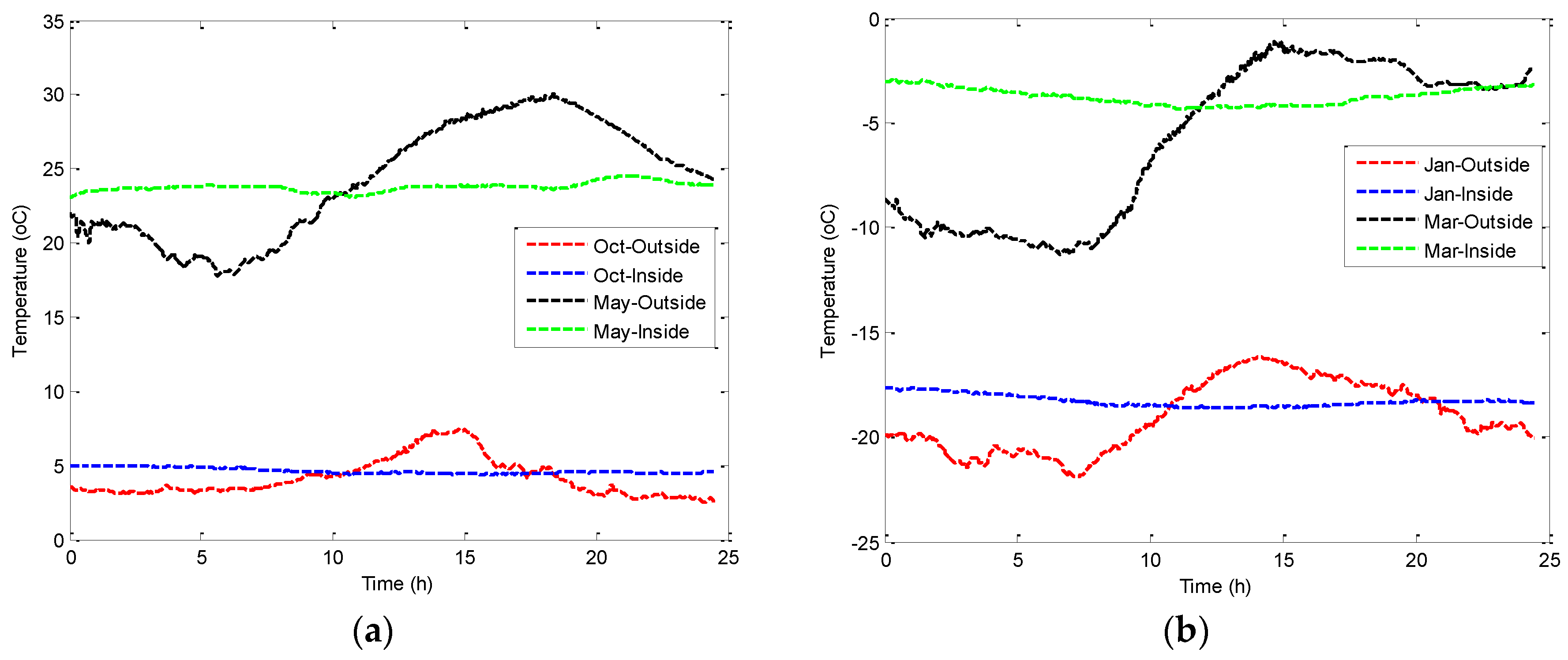
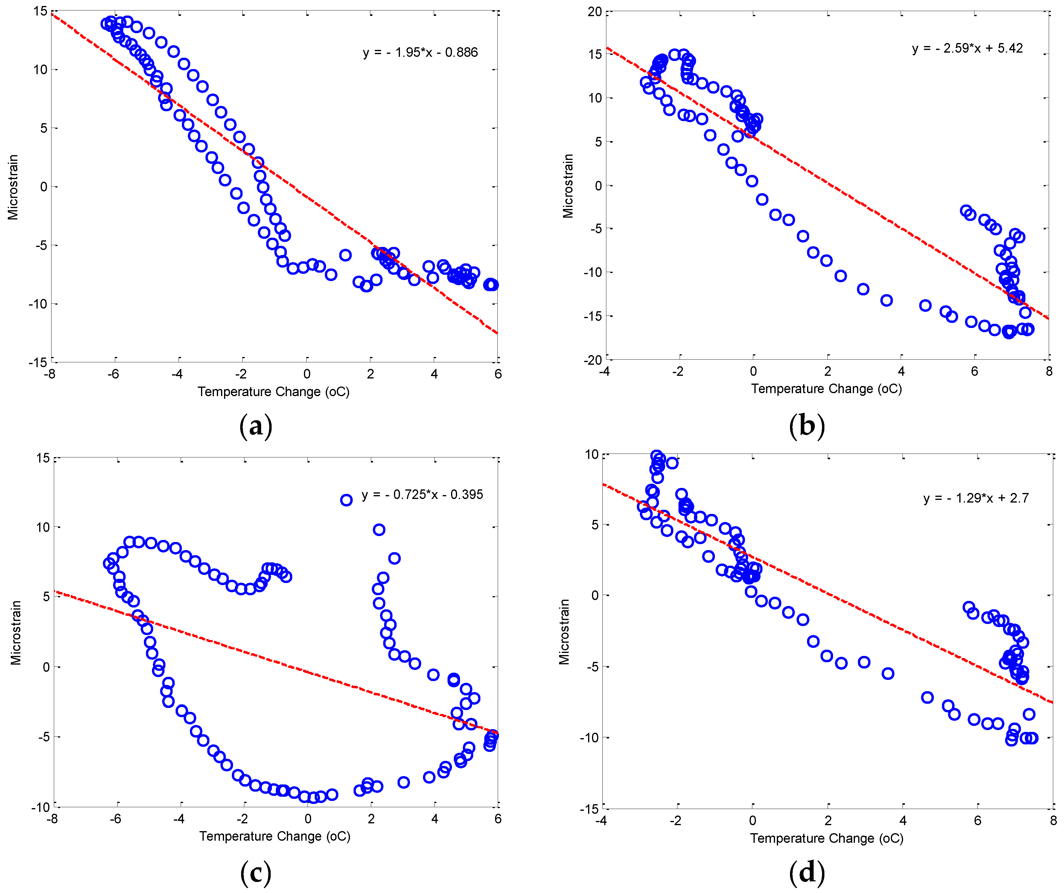
• The time-series correlation analysis of strain and temperature revealed that the winter temperature time has more effect on the upper and lower strain behavior than summer temperature, while the summer time strain behavior is less reliable than winter time, and the behavior of the bridge during winter time is more stable than summer time. Furthermore, the temperature changes of the bridge section affect the lower plate girder more than the upper plate during summer time. This means that the direct air temperature effect is higher than indirect temperature effects. The linear fitting between strain and temperature changes shows that the bridge performance during winter time is more stable than summer time.
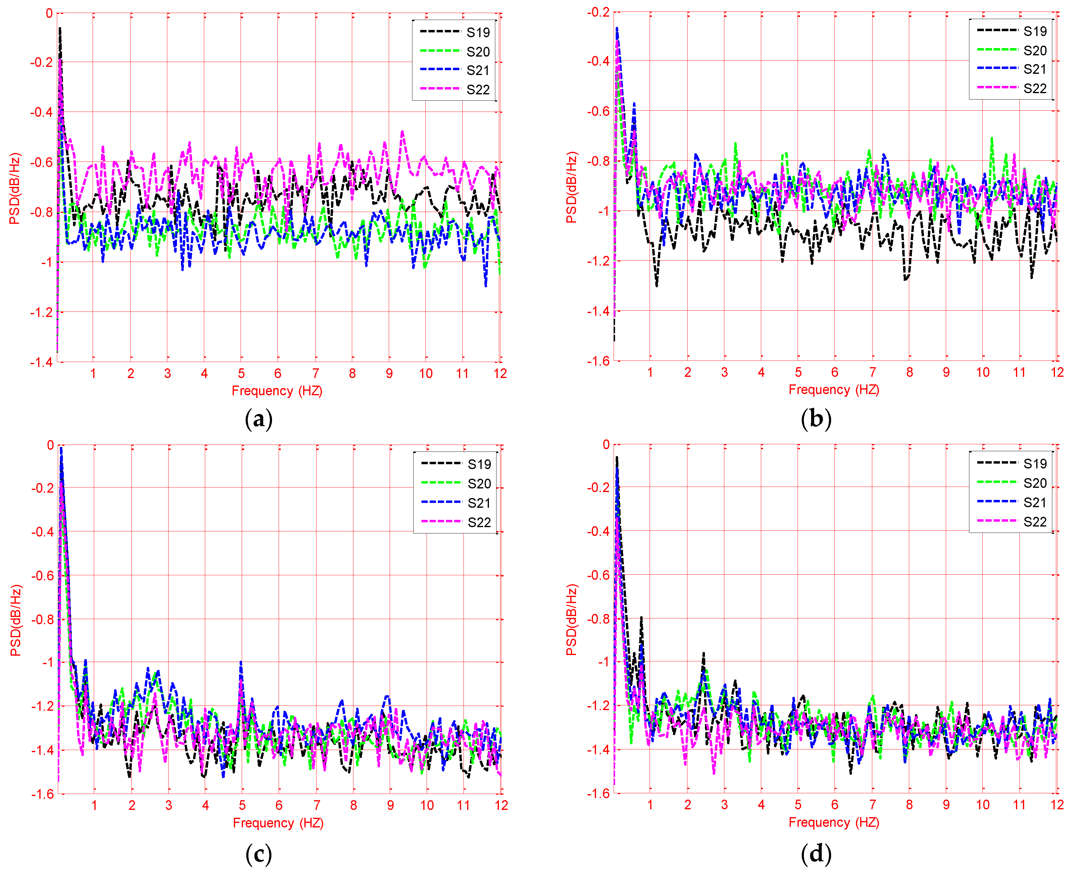
• The correlation of frequency spectrum analysis of strain residuals shows that the increased traffic volume on the bridge increases the bridge stability in vibration modes with more controlled bridge vibration. In addition, the air temperature and temperature changes of the bridge sections do not affect the frequency modes and power spectrum density of strain signals. The correlation of power spectrum density reveals that the dynamic performance of the bridge in summer and winter times is safe.

References

1. Xia, H. SHM-Based Condition Assessment of in-Service Bridge Structures Using Strain Measurement. Ph.D. Thesis, Department of Civil and Structural Engineering, Hong-Kong Polytechnic University, Hong Kong, China, 2011. [Google Scholar]
2. Dahal, S. Structural Health Monitoring for in-Service Highway Bridges Using Smart Sensors. Available online: http://digitalcommons.uconn.edu/gs_theses/381 (accessed on 5 May 2016).
3. Sohn, H.; Farrar, C.R.; Hemez, F.M.; Shunk, D.; Stinemates, D.W.; Nadler, B.R.; Czarnecki, J. A Review of Structural Health Monitoring Literature: 1996–2001; Los Alamos National Laboratory Report LA-13976-MS; Massachusetts Institute of Technology: Cambridge, MA, USA, 2004. [Google Scholar]
4. Miao, S.; Koenders, E.; Knobbe, A. Automatic baseline correction of strain gauge signals. Struct. Control Health Monit. 2015, 22, 36–49. [Google Scholar] [CrossRef]
5. Follen, C.; Sanayei, M.; Brenner, B.; Vogel, R. Statistical bridge signatures. J. Bridge Eng. 2014, 19, 04014022. [Google Scholar] [CrossRef]
6. Liu, M.; Frangopol, D.; Kim, S. Bridge system performance assessment from structural health monitoring: A case study. J. Struct. Eng. 2009, 135, 733–742. [Google Scholar] [CrossRef]
7. Ni, Y.; Xia, H.; Wong, K.; Ko, J. In-service condition assessment of bridge deck using long-term monitoring data of strain response. J. Bridge Eng. 2012, 17, 876–885. [Google Scholar] [CrossRef]
8. Howell, D.; Shenton, H. A system for in-service strain monitoring of ordinary bridges. In Structures Congress 2005; ASCE: New York, NY, USA; pp. 1–7.
9. Wang, G.X.; Ding, Y.L.; Sun, P.; Wu, L.; Yue, Q. Assessing static performance of the Dashengguan Yangtze bridge by monitoring the correlation between temperature field and its static strains. Mathemat. Probl. Eng. J. 2015, 2015, 946907. [Google Scholar] [CrossRef]
10. Omenzetter, P.; Brownjohn, J.M. Application of time series analysis for bridge monitoring. Smart Mater. Struct. 2006, 15. [Google Scholar] [CrossRef]
11. Hu, J.W.; Kaloop, M.R. Single input-single output identification thermal response model of bridge using nonlinear ARX with wavelet networks. J. Mech. Sci. Technol. 2015, 29, 2817–2826. [Google Scholar] [CrossRef]
12. Hong, C.; Bang, H.; Kang, H.; Kim, C. Real-time damage detection for smart composite materials using optical fiber sensors. In Proceedings of the 13th International Conference on Composite Materials (ICCM-13), CD-ROM ID-1509, Beijing, China, 25–29 June 2001.
13. Kaloop, M.; Elbeltagi, E.; Elnabwy, M. Bridge monitoring with wavelet principal component and spectrum analysis based on GPS measurements: Case study of the Mansoura Bridge in Egypt. J. Perform. Constr. Facil. 2015, 29, 04014071. [Google Scholar] [CrossRef]
14. Wu, B.; Li, Z.; Wang, Y.; Chan, T. Separation and extraction of bridge dynamic strain data Front. Archit. Civ. Eng. China 2009, 3, 395–400. [Google Scholar] [CrossRef]
15. Mata, J.; Casto, A.T.; Costa, J. Time-frequency analysis for concrete dam safety control: Correlation between the daily variation of structural response and air temperature. Eng. Struct. 2013, 48, 658–665. [Google Scholar] [CrossRef]
16. Xia, Y.; Chen, B.; Weng, S.; Ni, Y.; Xu, Y. Temperature effect on vibration properties of civil structures: A literature review and case studies. J. Civ. Struct. Health Monit. 2012, 2, 29–46. [Google Scholar] [CrossRef]
17. Chen, C.; Kaloop, M.R.; Wang, Z.L.; Gao, Q.F.; Zhong, J.F. Design of a long-term monitoring system for a PSC continuous box-girder bridge. Key Eng. Mater. 2014, 619, 1–9. [Google Scholar] [CrossRef]
18. Chen, C.; Kaloop, M.R.; Gao, Q.; Wang, Z. Environmental effects and output-only model identification of continuous bridge response. KSCE J. Civ. Eng. 2015, 19, 2198–2207. [Google Scholar] [CrossRef]
19. Kolev, V. Bridge Weigh-in-Motion Long-Term Traffic Monitoring in the State of Connecticut. Available online: http://digitalcommons.uconn.edu/gs_theses/838 (accessed on 5 May 2016).
20. Zhang, X.Z.; Rui, Y.Q.; Wang, W.X. An new filtering method in the wavelet domain for bowel sound. Int. J. Adv. Comput. Sci. Appl. 2012, 1, 26–31. [Google Scholar]
21. Rohatgi, A. Web Based Tool to Extract Data from Plots, Images, and Maps. Available online: http://arohatgi.info/WebPlotDigitizer/ (accessed on 5 May 2016).
22. Kaloop, M.R.; Li, H. Multi input-single output model identification of tower bridge movements using GPS monitoring system. Measurement 2014, 47, 531–539. [Google Scholar] [CrossRef]
23. Hasegawa, H.; Kanai, H. Frequency analysis of strain of cylindrical shell for assessment viscosity. Jpn. J. Appl. Phys. 2005, 44, 4609–4614. [Google Scholar] [CrossRef]
24. Li, S.; Wu, Z. Model analysis on micro-stain measurements from distributed long-gage fiber optic sensors. J. Intell. Mater. Syst. Struct. 2008, 19, 937–946. [Google Scholar]
25. Martin, H. Matlab Recipes for Earth Sciences, 2nd ed.; Springer: Berlin, Germany; Heidelberg, Germany; New York, NY, USA, 2007. [Google Scholar]
26. Mathworks Inc. MATLAB, Release 12; Mathworks: Natick, MA, USA, 2008. [Google Scholar]
27. Bigdeli, Y.; Kim, D. Damping effects of the passive control devices on structural vibration control: TMD, TLC and TLCD for varying total masses. KSCE J. Civ. Eng. 2016, 20, 301–308. [Google Scholar] [CrossRef]
Figure 1. Fu-Sui Bridge: (a) view; (b) monitoring system; and (c) bridge cross-section.
Ijgi 05 00061 g001
Figure 2. Measured temperature during the monitoring time.
Ijgi 05 00061 g002
Figure 3. Measured and smoothed data of: (a) strain of strain point S19; (b) temperature of May 2012.
Ijgi 05 00061 g003
Figure 4. Outside and inside cross-section temperature: (a) May and October 2012; (b) January and March 2013.
Ijgi 05 00061 g004
Figure 5. Section 5: (a) strain measurements; (b) wavelet filter of S19; and (c) traffic volume calculation (unit: number of vehicles).
Ijgi 05 00061 g005
Figure 6. Vehicle counts verification (a) strain measurements; (b) vehicle count.
Ijgi 05 00061 g006
Figure 7. Traffic counter flow chart.
Ijgi 05 00061 g007
Figure 8. Strain response variation for: (a) May 2012; (b) October 2012; (c) January 2013; and (d) March 2013.
Ijgi 05 00061 g008
Figure 9. Correlation scatter plots between S19 and S20 and temperature changes for the (a,b) S20 and (c,d) S19.
Ijgi 05 00061 g009
Figure 10. PSD of strain during: (a) May 2012; (b) October 2012; (c) January 2013; and (d) March 2013.
Ijgi 05 00061 g010