Article

Using Moderate-Resolution Temporal NDVI Profiles for High-Resolution Crop Mapping in Years of Absent Ground Reference Data: A Case Study of Bole and Manas Counties in Xinjiang, China

1
The State Key Laboratory of Remote Sensing Science, Institute of Remote Sensing and Digital Earth, Chinese Academy of Sciences, CAS Olympic S & T Park, No. 20 Datun Road, P.O. Box 9718, Beijing 100101, China
2
University of Chinese Academy of Sciences, No. 19A Yuquan Road, Beijing 100049, China
*
Authors to whom correspondence should be addressed.
ISPRS Int. J. Geo-Inf. 2016, 5(5), 67; https://0-doi-org.brum.beds.ac.uk/10.3390/ijgi5050067
Submission received: 15 March 2016 / Revised: 29 April 2016 / Accepted: 9 May 2016 / Published: 16 May 2016

Abstract

:
Most methods used for crop classification rely on the ground-reference data of the same year, which leads to considerable financial and labor cost. In this study, we presented a method that can avoid the requirements of a large number of ground-reference data in the classification year. Firstly, we extracted the Normalized Difference Vegetation Index (NDVI) time series profiles of the dominant crops from MODIS data using the historical ground-reference data in multiple years (2006, 2007, 2009 and 2010). Artificial Antibody Network (ABNet) was then employed to build reference NDVI time series for each crop based on the historical NDVI profiles. Afterwards, images of Landsat and HJ were combined to obtain 30 m image time series with 15-day acquisition frequency in 2011. Next, the reference NDVI time series were transformed to Landsat/HJ NDVI time series using their linear model. Finally, the transformed reference NDVI profiles were used to identify the crop types in 2011 at 30 m spatial resolution. The result showed that the dominant crops could be identified with overall accuracy of 87.13% and 83.48% in Bole and Manas, respectively. In addition, the reference NDVI profiles generated from multiple years could achieve better classification accuracy than that from single year (such as only 2007). This is mainly because the reference knowledge from multiple years contains more growing conditions of the same crop. Generally, this approach showed potential to identify crops without using large number of ground-reference data at 30 m resolution.

1. Introduction

Multi-temporal remote sensing data can be used to describe changes in vegetation characteristics over time [1,2,3], and these data have been employed to produce crop distributions from regional to national scales using both, supervised and unsupervised classifiers [4,5,6,7,8,9,10]. Moreover, the crop maps are the foundation for crop modeling, irrigation water distributions and land water management, which are important for decision makers [11,12,13,14,15]. However, most of the previous studies relied on the field reference data in the mapping year to train the classifiers [16,17]. When the cropland map need to be provided on yearly basis, the ground-reference data will be collected at annual frequency, which leads to considerable financial, time and labor costs [18]. In addition, national or local authorities do not pay much attention to collecting ground-reference data sometimes, which lead to the difficulties in obtaining the ground reference data annually [19].
In areas with a stable cropping system, phenological metrics of the same specific crop are usually more similar than that of different crops among multi-years [18,20,21]. Thus, vegetation indices (VI), such as Normalized Difference Vegetation Index (NDVI) and Enhanced Vegetation Index (EVI), time series and the phenological metrics extracted from the VI time series have been used to transfer the knowledge of training samples from one year to another [21,22,23,24,25]. On the one hand, coarse spatial resolution data (such as Advanced Very High Resolution Radiometer, AVHRR and Moderate Resolution Imaging Spectroradiometer, MODIS), which are characterized by density temporal resolution, have shown the potential to identify crop types using the classification model built from the adjacent years [21], whereas a drawback is the relatively coarse spatial resolution cannot discriminate crop types in heterogeneous landscape [26,27,28,29]. Some pixel unmixing attempts, which are based on both linear and non-linear regression principles, have been proposed to solve this situation [30,31,32,33], but there are still some limitations: (1) the unmixing approaches can solely derive sub-pixel fractions of crop area in a pixel, and hardly provide the crop distribution within the pixel; (2) the VI profiles of some crops maybe too similar to be reliably separated; and (3) if the endmembers were extracted across multiple years, the inter-annual differences will result in the variable temporal signatures of endmembers of the same crop [30].
On the other hand, the image time series at finer spatial resolution, such as Landsat Thematic Mapper (TM) and Satellite Pour l’Observationde la Terre (SPOT), have shown the potential to discriminate crops [5,15,34]. Note that there have been some attempts at identifying crop types without ground reference data of the classification year using the spectrum at specific phenological periods [22,23]. The limitation of these methods is that they have to extract phenological metrics using high resolution image time series (such as Landsat) in the classification year, which result in the difficulty of the application of these methods in large area for the following reasons: (1) within one year, it is difficult to obtain cloud-free image time series that are dense enough to extract phenological metrics in large areas by a single sensor (such as Landat 5); and (2) although the temporal resolution of the image time series can be improved by combining the data from multi-sensor [35,36], the radiometric differences among different sensors may have negative influence on the accuracy of the phenological metrics [37].
The objective of this study is to propose a method and classify crop types at high resolution (30 m) without the use of the ground reference samples in the classification year. To achieve this purpose, we combined the advantages of both moderate resolution (MODIS) and high resolution (Landsat and Huan Jing) data. First, we acquired the historical ground reference data of multiple years (2006, 2007, 2009 and 2010); the NDVI profiles of the crops were extracted from MODIS NDVI time series using historical ground reference data; and reference NDVI time series were then obtained from the historical NDVI profiles. Afterwards, the linear relations between Landsat/HJ NDVI and MODIS NDVI during the entire crop-growing season were obtained, and the reference NDVI time series were transformed using the linear relations. Finally, the transformed reference NDVI time series were utilized to identify crop types at 30 m resolution.

2. Study Regions and Data Description

2.1. Description of the Study Area and the Crop Calendar

In this study, we selected two representative agricultural regions in northern Xinjiang, Bole County and Manas County. Bole County (44°20′~45°23′N, 80°40′~82°42′E) covers 32 kha of cropland (Figure 1a), and the average temperature and rainfall is 14.1 °C and 144.4 mm during the crop period (between April and October), respectively. Manas County (43°17′~45°20′N, 85°17′~86°46′E) covers 180 kha of cropland (Figure 1a), the average temperature and rainfall are 14.4 °C and 153.2 mm during the crop period, respectively.
Cropland covers 13.7% (more than 1100 ha) and 15.8% (more than 1800 ha) of the total area in Bole and Manas, respectively. The dominant crops grown in the study areas include cotton, spring maize, watermelon, grape, tomato, and wheat. The vegetation cover fraction for each crop type over the course of a year is presented in Figure 1b. Cotton, spring maize, watermelon, tomato, and grape are planted in early April and begin their growth mostly during the June–July period. Watermelon and tomato are harvested in August, spring maize is harvested in early September, and grape and cotton are harvested during the August–September and September–October periods, respectively. However, the field for winter wheat is a bit complex. Winter wheat is planted in early November, begins its growth in the next April, and is reaped for harvest in late June. After the harvest, some fields are in rotation, and others are used to plant some other summer crops, mainly summer maize. Hence, we divided the winter wheat into two parts relying on whether summer crops are planted in the same field or not.

2.2. Datasets

2.2.1. MODIS Imagery

Sixteen-day composite Terra MODIS 250m NDVI data from the MOD13Q1 Vegetation Indices product were used in this study. These data were downloaded from Land Processes Distributed Active Archive Centre [38], and two MODIS tiles (h23v04 and h24v04) were used to cover all of the field sites. The MODIS NDVI images are consisted of 15 scenes (21 March–1 November) in each year and spanned five crop years (2006, 2007 and 2009–2011). The MODIS images were mosaicked and re-projected from Sinusoidal to UTM WGS84 zone 44N (Bole) and zone 45N (Manas).

2.2.2. TM and HJ-CCD Imagery

Images used in this study are listed in Table 1 and Table 2. Data from both Landsat TM/ETM+ and Huan Jing (HJ) CCD with cloud-cover of less than 10% were used to acquire the time series at 30 m spatial resolution. The HJ-1 Constellation has two satellites (HJ-1A and HJ-1B), and each satellite had two CCD cameras. Compared with Landsat TM images, HJ data have similar spatial resolution (30 m), and finer temporal resolution (four days). Table 3 shows the spectral range of Landsat-5 TM and HJ-1 CCD in Red and Near-Infrared (NIR) bands, which were used to calculate NDVI.
The Landsat-5 TM surface reflectance product (CDR) and the HJ Level 2 standard product (DN value) were used to classify crop types in 2011 at 30 m resolution in this study [39,40]. Images were georeferenced to the UTM WGS 84 zones 44N (Bole county) and 45N (Manas county). The HJ images were registered to the TM images, achieving a RMSE of less than 0.3 pixels using a 2nd order polynomial transformation and bi-linear resampling. Subsequently, radiance calibration and FLAASH atmospheric correction were performed for HJ-1 CCD images [41]. Normalized Difference Vegetation Index (NDVI) time series was employed in this study, and we used Red and NIR bands to calculate NDVI (Equation (1)).
NDVI = ρ ( NIR ) ρ ( Red ) ρ ( NIR ) + ρ ( Red )
where ρ ( NIR ) and ρ ( Red ) were the land surface reflectance of the NIR band (0.775~0.9 μm) and Red band (0.63~0.69 μm), respectively. As for the Landsat-5/7 data during 2006 and 2010, we used the original images with DN value because these images were just utilized to identify crop fields containing entire MODIS pixels.

2.2.3. Ground-Reference Data

In this study, the ground-reference data were divided into two parts: historical field samples used for building reference NDVI time series across four years (2006, 2007, 2009 and 2010), and field samples used for validating classification accuracy in 2011. The distribution of the ground reference data is shown in Figure 2.
To obtain the historical field samples, we selected 33 and 30 sampling frames (1 km by 1 km) in Bole and Manas, respectively. Then, NDVI of all Landsat images during 2006 and 2011 were calculated, and the field boundaries were visually interpreted in each sampling frame based on the 30 m NDVI images of each year. Afterwards, the field boundaries were overlaid on the MODIS images, and the fields that did not contain entire MODIS pixels were removed. The crop type information during 2006 and 2010 of the remained fields was obtained from the local statics Bureau and farmers during the field survey work in 2011. Subsequently the historical NDVI time series were extracted from pure ground reference MODIS pixels. If there were more than 13 “good data” periods in a reference pixel among the “Pixel Reliability” of the 15 time periods [38], the pixel was retained. Otherwise, the pixel was removed from the historical reference dataset. For the remaining pixels, the NDVI for low-quality periods (if the quality of a pixel is not “good data”, we define it as “low-quality”) was replaced by the average NDVI of the previous and following periods. Finally, there were 1061 samples of the seven major crop types in the study area in total (Table 4). We did not collect the historical field samples in 2008 because we did not obtain Landsat-5 TM images in 2008 before our field survey. Thus, the crop types of 2008 were not retrieved during the farmer interview. The procedure for obtaining the historical ground reference samples is shown in Figure 3.
The validation field samples were collected by field research of the study area during 2011. These field samples were selected to represent the full variety of crop types and an even distribution across the study areas. A total of 525 fields in Bole and 463 fields in Manas were selected and surveyed. For each field, the crop type was collected as attribute information. Field boundaries were recorded using GPS, and digitized as polygons. All polygons were converted to raster format using the TM grid (30 m spatial resolution), and boundary pixels were removed to ensure that all samples are pure crop pixels. In addition, the polygons were overlaid on the MODIS grid (250 m resolution), and the MODIS pure pixels were obtained. To compare the results derived from historical reference with that derived from the ground-reference data, some of the samples were used as training samples. The number of training and validation samples is shown in Table 5.

3. Methods

The methodology of the study was presented in 
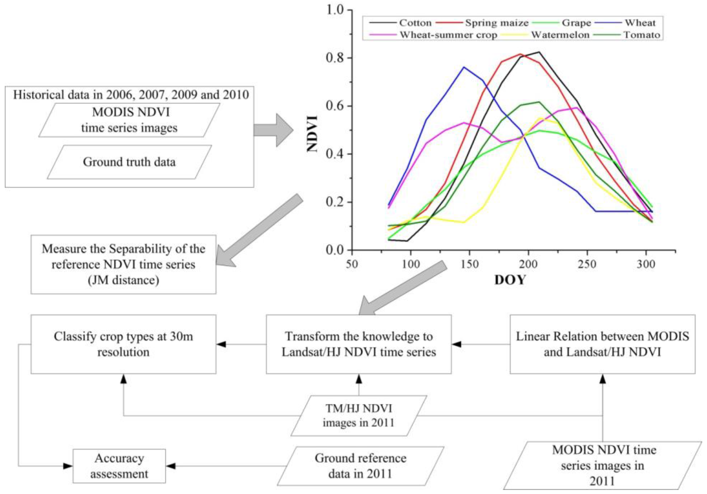
Figure 4. This study was composed of six main parts: (1) extracting NDVI time series profiles from MODIS data using ground reference data in 2006, 2007, 2009 and 2010; (2) building historical reference NDVI time series (between 2006 and 2010) for each crop using ABNet based on the historical NDVI time series profiles, and measuring the separability of reference NDVI for crop classification; (3) using Landsat-5 TM and HJ data to build multi-source NDVI time series at 30 m resolution in 2011; (4) testing the linear relationship between Landsat/HJ and MODIS NDVI, and then transforming the reference NDVI time series using the linear relation; (5) using the transformed reference time series to classify crop types at 30 m spatial resolution; and (6) assessing classification accuracy. Additionally, the classification accuracy was compared with the result derived from ground-reference data of 2011.

3.1. Artificial Antibody Network

The Artificial Antibody Network (ABNet) was proposed by Zhong and Zhang [42] based on artificial immune network principles (AIN). The antibody model was used as the basic component for the ABNet and each antibody contained three attributes: the crop type of the antibody, center vector and the recognizing radius. The ABNet have two procedures: training and classification. During the training procedure, the training antigens were used as input of the ABNet, and the antibodies were obtained. Then, in the classification procedure, the antibodies were used to identify new antigens.
The training procedure of the ABNet contained five steps for each class: pre-selection, cloning, mutation, adaptive calculation of new antibodies and antibody reorganization. The detailed training process can be found in work of Zhong and Zhang [42]. While training the ABNet, an important issue was to select a similarity measure, and we used Euclidean distance (Equation (2)) [43], which can easily measure the similarity in the training process:
ED ( a , b ) = t = 1 n ( a t b t ) 2
where a t and b t are the values of time series a and b at moment t, respective, and N is the number of samples in the time series. Moreover, the ABNet can build up a network and guarantee its convergence adaptively, and no more parameters need further optimized.
The classification procedure was to calculate the Euclidean distance between vector of a new antigen and the center vector of each antibody, and the new antigen was labeled as the crop type of the antibody with the minimum distance if the minimum distance was less than the recognizing radius of the antibody. Otherwise, the spectral angle (Equation (3)) was calculated between the vector of the new antigen and the center vector of the antibodies [44], and the antigen was labeled as the crop type of antibody with the minimum spectral angle.
SAM ( a , b ) = cos 1 ( t = 1 n ( a t · b t ) t = 1 n ( a t ) 2 t = 1 n ( b t ) 2 )
We employed ABNet in this study to build the reference NDVI time series for each crop because ABNet can adaptively build up the network and guarantee its convergence without any parameters. In addition, one crop type can contain many antibodies, and the ABNet could recognize different distinctive patterns that are suitable for identifying the same crop in different situations with variable NDVI time series. In this study, the ABNet was interpreted in IDL.

3.2. Building the Reference NDVI Time Series for the Crops

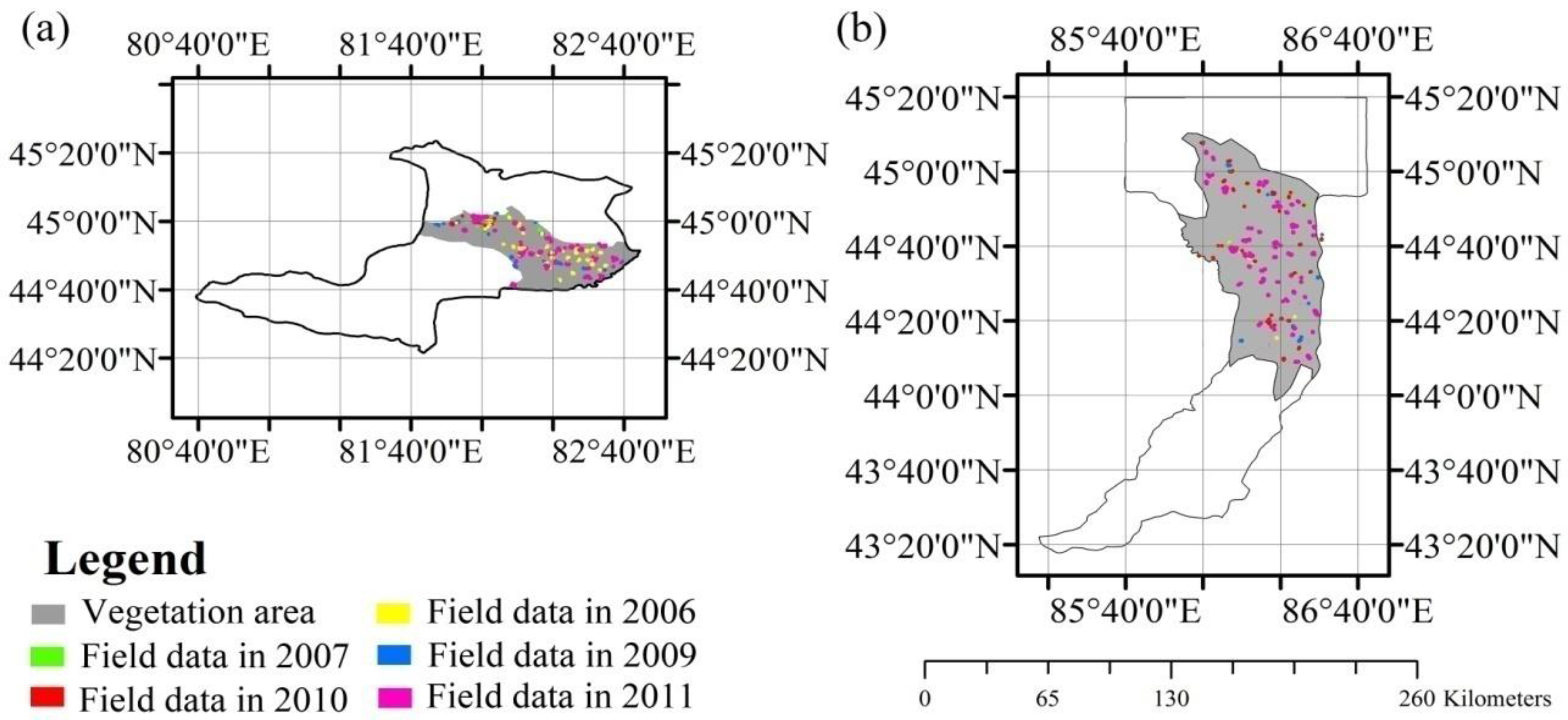
We used the ABNet to build the reference NDVI time series. First, we extracted the NDVI time series from the ground reference samples of both Bole and Manas. Then, all historical NDVI profiles were used as input of the ABNet training process, and the antibodies were then obtained. The center vectors of the antibodies were the reference NDVI time series for each crop type, and multiple reference NDVI time series profiles were obtained to describe the same crop under different conditions.

3.3. Measuring the Separability of Reference NDVI Time Series

In this study, we used the Jeffries-Matusita (JM) distance to measure the separability of the reference NDVI time series for each pair of crops because previous studies showed that JM distance could better measure the separability among different classes than other distances, such as Euclidean distance or divergence [41,45]. The JM distance between a pair of class and specific functions was given by:
JM ( c i , c j ) = x ( p ( x | c i ) p ( x | c j ) ) 2 dx
where x denotes a span of VI time series values and c i and c j (lowercase c) denote the two crop classes under consideration. Under normality assumptions, Equation (2) was reduced to JM = 2 ( 1 e B ) , where:
B = 1 8 ( μ i μ j ) T ( C i + C j 2 ) 1 ( μ i μ j ) + 1 2 ln ( | | C i + C j | 2 | C i | × | C j | | )
and C i and C j (uppercase C) are the covariance matrixes of class i and j, respectively. Additionally, | C i | and | C j | are the determinants of C i and C j , respectively. The JM distance ranged from 0 to 2, with a large value indicating a high level of separability between two classes [46].

3.4. Testing the Relation between MODIS and Landsat/HJ NDVI

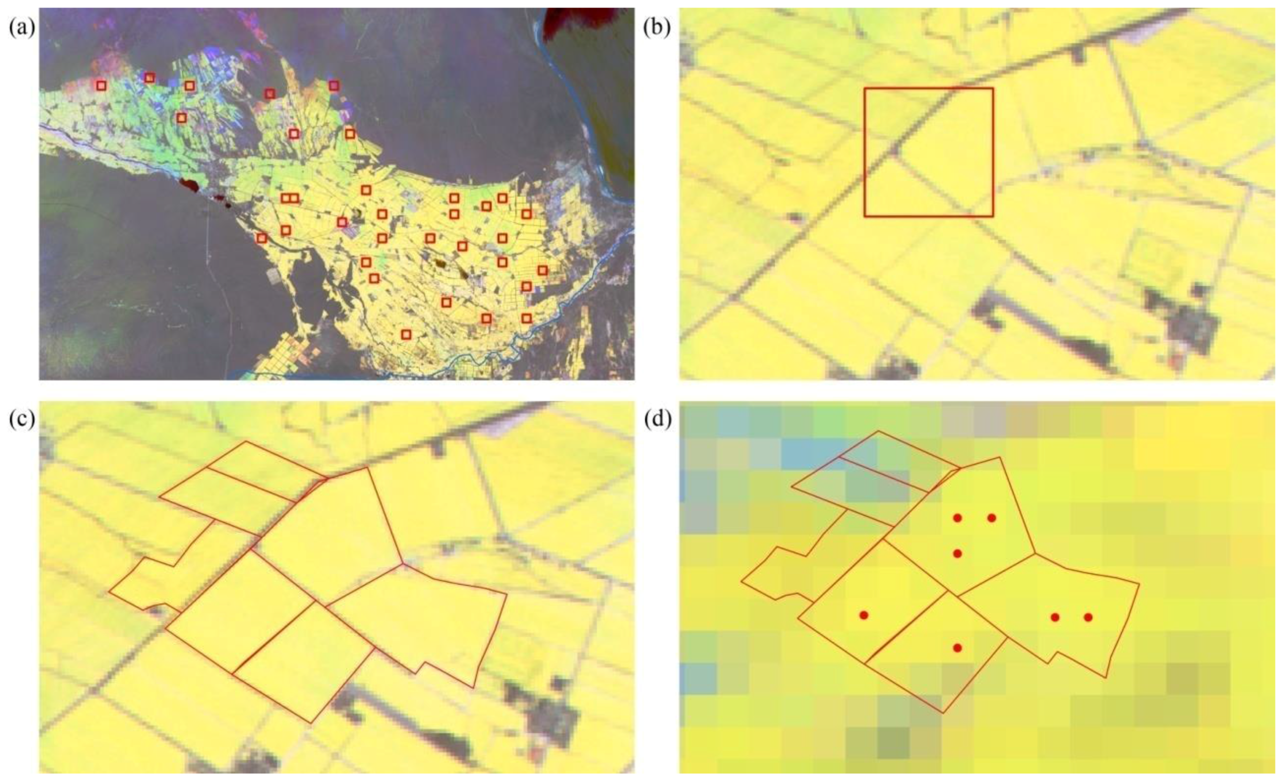
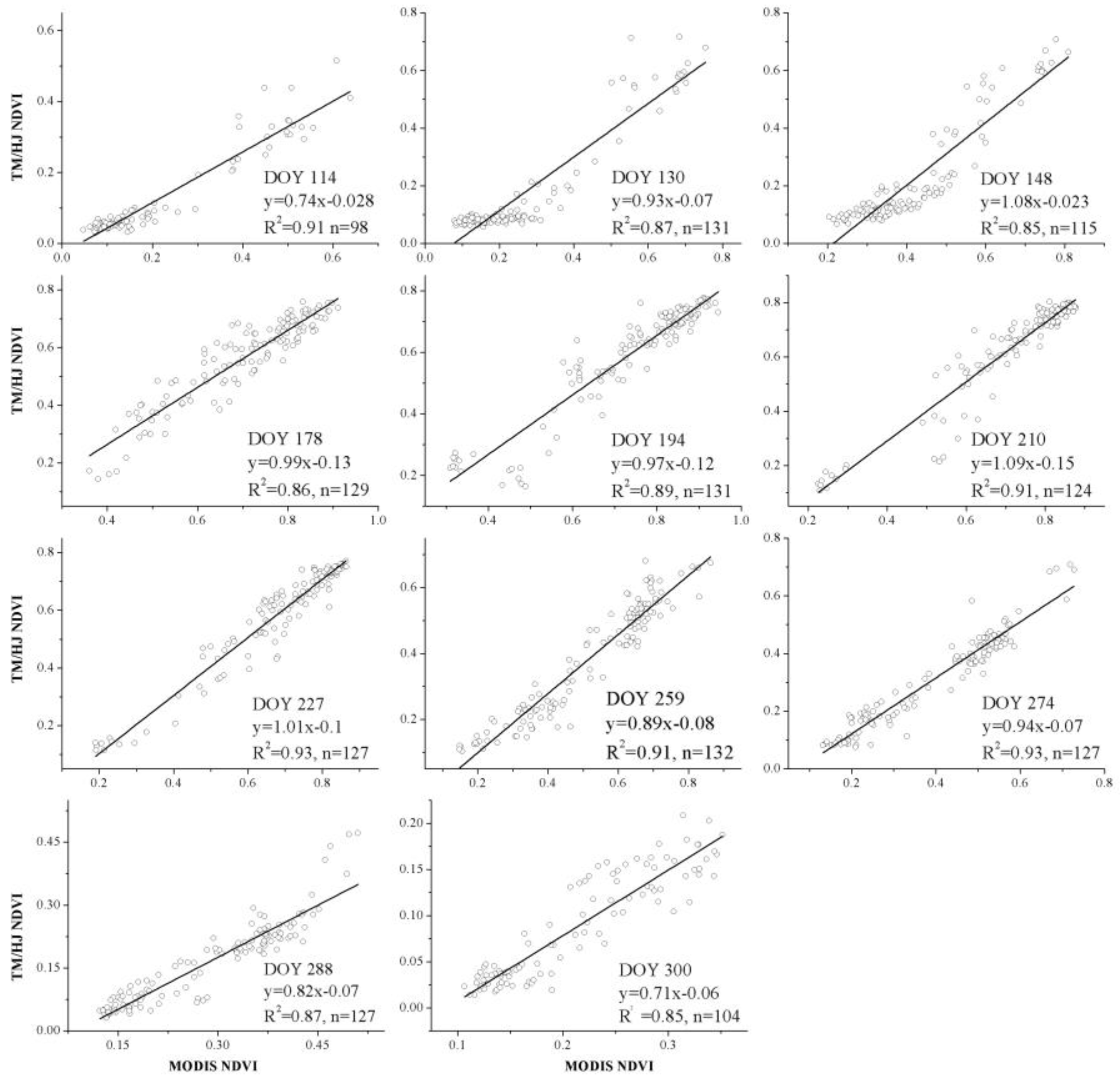
We combined the Landsat-5 TM and HJ-1 NDVI in 2011 to increase the temporal resolution of NDVI time series at 30 m resolution. For each Landsat TM/HJ CCD NDVI image, we selected the MODIS image whose temporal flag is the nearest to the date that Landsat TM/HJ CCD images were acquired. When testing the relationship between Landsat TM/HJ CCD NDVI and MODIS NDVI, the samples were selected in homogenous crop fields, and the average NDVI of all Landsat TM/HJ CCD pixels to the corresponding MODIS pixel were calculated. Coinciding with some previous studies, Landsat TM/HJ CCD NDVI and MODIS NDVI showed strong linear relationships (R2 > 0.8 in Figure 5 and Figure 6) [37,47,
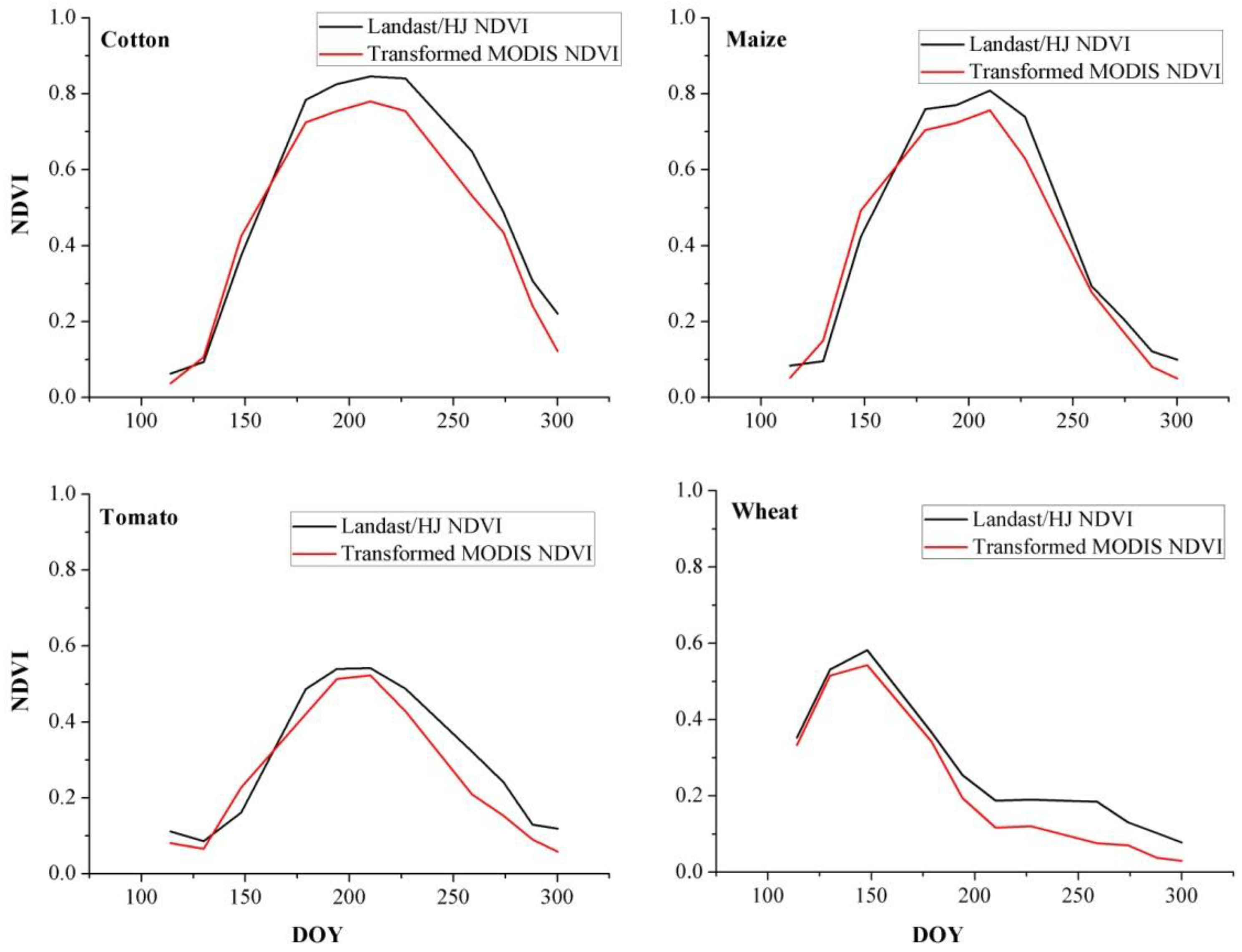
48]. Then, all reference NDVI time series were transformed to Landsat/HJ NDVI using corresponding linear relation, and the transformed reference NDVI time series were used to identifying crop types in the next step.

3.5. Crop Classification at 30 m Resolution

We first masked the non-agricultural area using the “agriculture land” of Finer Resolution Observation and Monitoring of Global Land Cover (FROM-GLC) at 30 m spatial resolution [49]. Before the masking, we randomly selected 300 validation pixels in both study regions using Hawths Tools [50]; all validation samples were visually interpreted as crop/non-crop (Table 6), and these validation samples were used to verify the accuracy of the crop mask. The overall accuracies were above 90% for both study areas, which indicated that the crop mask of both study regions were accurate enough to mask non-crop area. Next, we classified the crops at 30 m resolution using the transformed reference NDVI time series by the classification procedure of ABNet. In addition, we used a portion of the ground-reference data as training samples to classify the agricultural area for comparison. The classifier was also ABNet.

4. Results

4.1. Reference NDVI Time Series

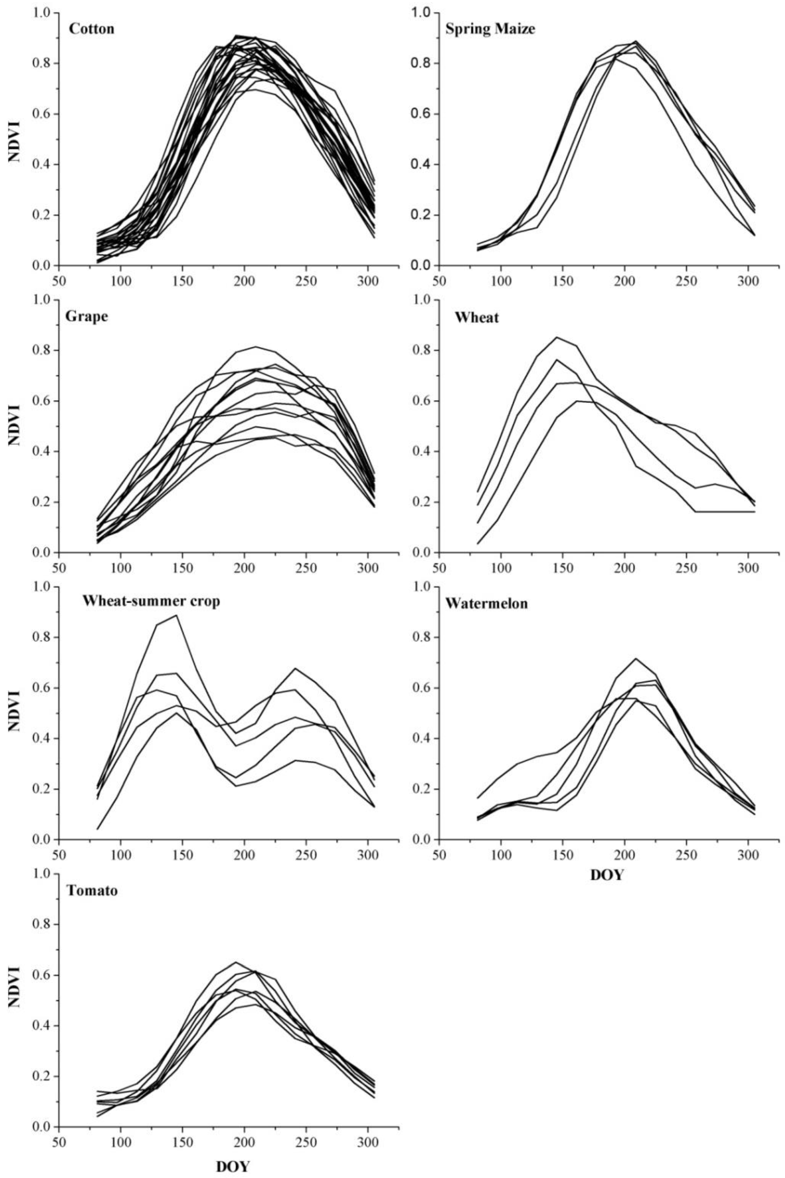
For each crop type, the reference NDVI time series were plotted in 
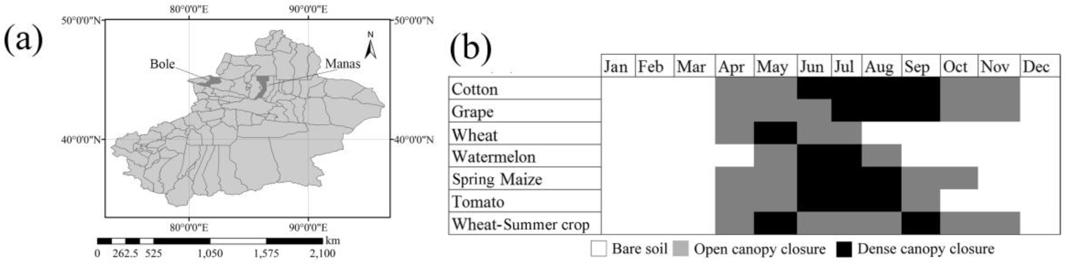
Figure 7. Among the summer crops, cotton was the major crop type in the study region, and had the largest amount of reference NDVI time series among all crops. The highest NDVI value of cotton was between 0.75 and 0.9 around Day 190 (late July). For spring maize, the highest value was similar to cotton, but after the peak, NDVI of spring maize decreased faster than cotton, and at around Day 250 (September), NDVI of spring maize was relatively lower than cotton. Tomato also had the highest NDVI around Day 190, but the NDVI value was between 0.5 and 0.6, which was significantly lower than cotton and spring maize. For grape, NDVI was high during Days 170–250 (from late June to early September). In addition, the variability of grape was the largest among all crops in the study region (between 0.4 and 0.7). Another summer crop was watermelon, which had a relatively short growing season, with NDVI peak at around Day 210 (late July). The major winter crop in the study areas was winter wheat, the time period of high NDVI (above 0.5) value was between Days 120 and 130. After the harvest of the winter wheat, some filed were used to plant the summer crops. The crops were sown at about Day 200 and then reach NDVI peak between Days 230 and 270. As there are various crop types, the NDVI profile differed, while we did not identify the summer crop types and just labeled all pixels with a NDVI peak after the harvest of wheat as wheat-summer crop.
Period-by-period JM distances were calculated using the reference NDVI time series of different crop types. The result (Figure 8) showed that the winter wheat and wheat-summer crop can be distinguished from the other crops between day 120 and 140 with the early NDVI peak. In addition, wheat could be discriminated from wheat-summer crop at day 170 because of the development of the summer crops. Grape had the lowest separability among all crops, and the average JM distance between grape and all other crops were around 0.5 in each time period. This was attributed to the large variability of the reference NDVI time series of grape. For example, some grape reference profiles had low NDVI, but some other grape reference time series had high NDVI values, which were similar to the cotton profiles. Moreover, cotton and spring maize had relatively low separability (1.994 in Table 7) because of the similar NDVI during the majority of the growing season (between Days 81 and 225 in Figure 8), and the similarity between cotton and spring maize was also observed by [51,52] in Uzbekistan. Generally, JM distances for all pair-wise crop comparisons were above 1.9 when all time periods in the entire growing season were used (Table 7), which indicated that the reference NDVI time series of each crop was separable in the study region.

4.2. Classification Accuracy Assessment

The results of the accuracy assessment (overall accuracy, Kappa coefficient, user’s and producer’s accuracy) for the two study areas are summarized in Table 8 and Table 9 [53,54]. If the historical NDVI time series of single year is used to build the reference NDVI profiles, the classification accuracies were low. For example, when the historical NDVI time series of 2007 were used to build the reference NDVI time series, the overall accuracy was 73.01%. The summer crops, such as spring maize, watermelon and grape were seriously mislabeled as cotton. Moreover, the reference tomato NDVI time series were not collected in 2006 and 2007; as a result, the reference profiles obtained from only 2006 and 2007 cannot identify tomato in 2011.
When the historical NDVI time series among 2006 and 2010 were used to build the reference time series, the classification accuracy improved significantly. The overall accuracy in Bole and Manas were 87.13% and 83.48%, respectively, which were acceptable for crop mapping without the use of ground reference data in the classification year. In Bole, both producer’s and user’s accuracy (PA and UA) of cotton, watermelon, wheat and wheat-summer crop were above 80%; but PA and UA of grape were about 70% because cotton and grape were confused: 280 cotton pixels were mislabeled as grape, while 260 grape pixels were wrongly classified as cotton. Spring maize had low UA (70.16%) because more than 200 cotton pixels were labeled as spring maize. In Manas, PA of cotton, spring maize, wheat and wheat-summer crop were higher than 80%, but the UA of spring maize and wheat were low (only 71.54% and 65.43%, respectively) because 272 and cotton samples were mislabeled as spring maize and wheat, respectively.
To assess the quality of the classification process based on the historical reference NDVI time series, a portion of the ground-reference data were used to classify the crops using the same classifier (ABNet). The overall accuracies for Bole and Manas were found to be 90.21% and 86.87%, respectively, which were higher compared to the accuracies for the historical reference NDVI-derived classification. In Bole, the increase of the accuracy was mainly caused by the better identification of wheat and wheat-summer crop (both PA and UA of wheat and wheat-summer crop were higher than 98%). In Manas, more correctly classified cotton and tomato pixels contributed to the improvement of the overall accuracy.
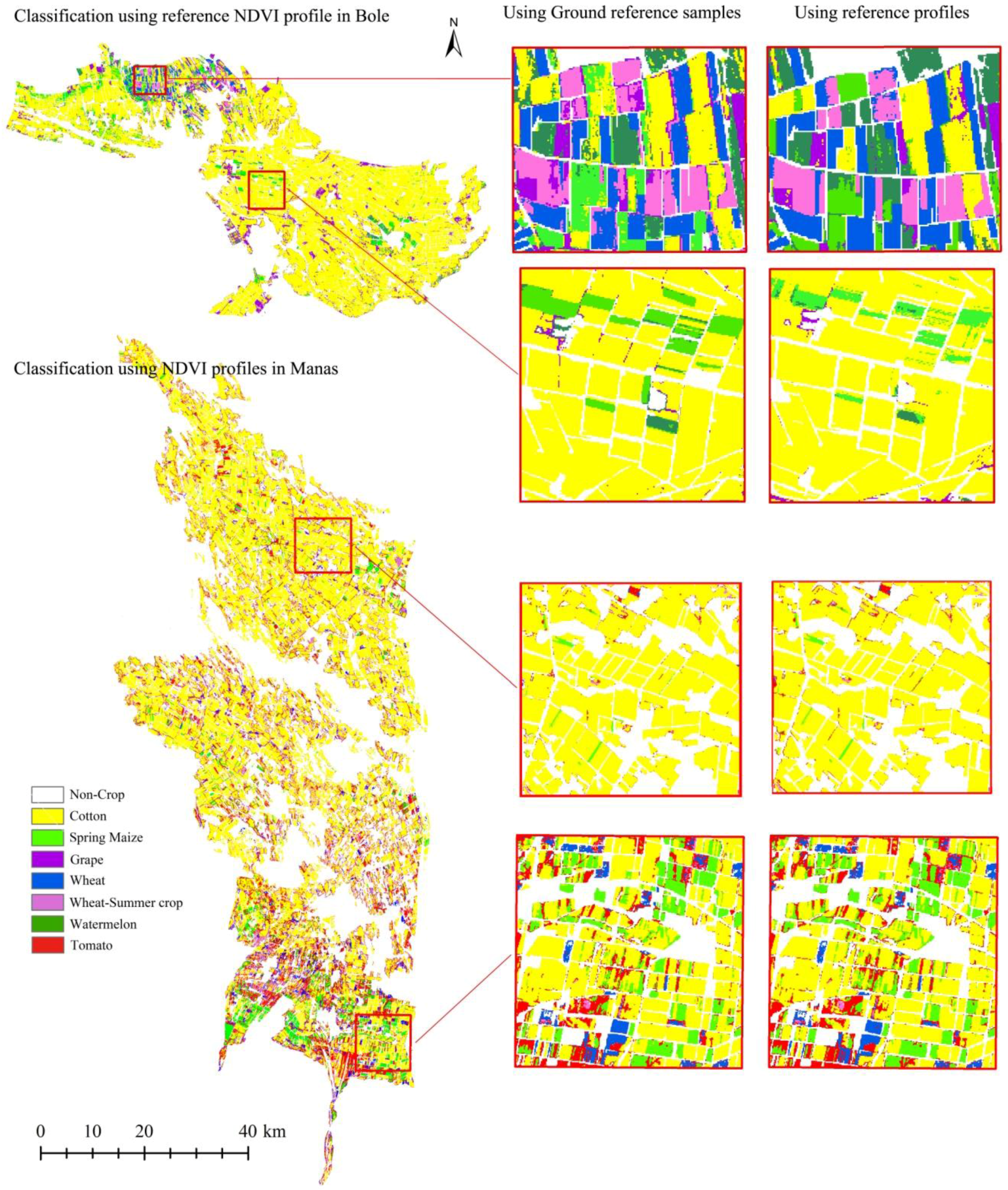
Figure 9 shows the crop map in Bole and Manas for year 2011. Cotton was the major crop type in both study areas, comprising 67.79% and 62.68% of cropland in Bole and Manas, respectively. In Bole, cotton was mainly distributed in the central county, and spring maize was mainly planted in the northwest of the county. Other crops, such as grape and watermelon were planted in the northern county. In Manas, cotton was mainly planted in the central and northern counties; and spring maize was planted in the southern county. As the crop identification were conducted at pixel level, there were some inter-field misclassifications, which was mainly due to the crop situation variation. In addition, the field boundaries were always misclassified. This was mainly because the boundary pixels were always mixed pixels combining crops and the road beside the crop fields. The mixed NDVI signature was perhaps more similar to the NDVI of a different crop, which led to the misclassification. As the training and validation samples did not contain field boundary pixels, these misclassification were not reported in the accuracy assessment confusion matrix.

5. Discussion

This study uses the knowledge acquired from historical ground reference data and MODIS image time series to replace the ground reference in the classification year and classify the crops at 30 m resolution. The separability tests (JM distance) of the reference NDVI time series have shown that the crops in the study area are separable (Table 7). But the challenges of using the reference NDVI time series to identify crops at 30 m resolution contain the following three aspects: (1) the observation frequency of high resolution sensors; (2) the variation of the phenological metrics may result in the situation that the reference profiles cannot identify the crops in the classification year; and (3) the NDVI transformation (using linear relation to transform MODIS to Landsat/HJ NDVI) may attribute to some uncertainty in crop identification.

5.1. The Combination of Landsat and HJ Images

The reference NDVI profiles in this study are obtained from the MODIS 16-day composite NDVI product, and the reference profiles have shown the potential to separate the crops in the study area. However, for the images time series at 30 m spatial resolution, the first challenge is the temporal resolution of the image time series. Previous studies have indicated that some optimal time periods could classify the crop types with high accuracy and using more images provide little further improvement for the crop identification [35,55,56]. For the images from a single sensor at 30 m resolution, such as Landsat, the possibility of acquiring cloud-free images in each season is limited to only about 50% during winter and fall, and 60% during summer and spring on average [57]. Apparently, this relatively low image acquiring frequency cannot fulfill the requirement of the crop classification. In this study, we combined Landsat and HJ images and obtained the image time series of nearly 15-day temporal resolution. The combined images time series could classify the crops with high accuracy (the overall accuracy of using ground reference to classify crops is found in Table 8 and Table 9), which is also consistent with other studies that the combination use of the images from multi-sensor could benefit the crop classification procedure, especially in large areas [58].

5.2. The Influence of Crop Growth Situation Variation on Crop Identification

Another challenge for crop identification using reference knowledge is the inter-annual phenological changes of the crops caused by the variation of temperature and precipitation among multiple years [43,59,60,61]. The temporal patterns of NDVI (Figure 10) have shown inter-annual variation in Bole and Manas. The NDVI time series of cotton among the five years are similar generally, except for slight variations during DOY 225~300. For spring maize, the NDVI peak of the profiles in all years are similar, the inter-annual variations are mainly in spring (DOY 100~150) and autumn (DOY 225~300). Grape and wheat have greater inter-annual variation, the NDVI of grape in 2007 is significantly higher during the entire growing season, and the wheat profiles showed that both greenup and NDVI-peak phases are 20 days earlier in 2007 than in the other years. In addition, NDVI peaks also vary by 0.06 and 0.11 for grape and wheat, respectively.
When using historical data of a single year as reference knowledge, the classification accuracies vary significantly. If the crop conditions of the reference year and the classification year are similar, the reference knowledge could achieve acceptable accuracy (such as using reference data of 2010 in Bole, Table 8). Otherwise, the reference knowledge and the NDVI pattern of the classification year are mismatched, and the classification accuracies are low (such as using reference data of 2007 in Manas, Table 9). Some complex methods have been proposed to use the shape of the NDVI profiles to measure the similarity [62]; but the shape of the NDVI time series sometimes changes because of the inter-annual phenological variation [43], which may lead to the failure of the shape-based similarity measures. Note that historical NDVI series from multiple years are used in this study, and reference knowledge from multiple years contains more growing conditions of the same crop and improves the classification performance when compared with the reference knowledge from a single year (Table 8 and Table 9). However, there is a limitation: if the crop condition has not been recorded in the reference knowledge, this method may fail to correctly identify crops. Therefore, we need to collect as much historical reference data as possible to enrich the knowledge of reference NDVI time series.
We select ABNet in this study because maybe the principle of ABNet is suitable for the acquisition of reference NDVI time series. The NDVI profiles of all samples among multiple years are used to derive the antibodies. Thus, each antibody could represent a specific phenological condition of one crop. Therefore, different distinctive patterns of the same crop are recorded by ABNet. Additionally, another advantage of ABNet is that it is an adaptive classifier, which needs no user-defined parameters during the training procedure.

5.3. The Influence of NDVI Transformation

In this study, we used MODIS NDVI time series as a reference, and transformed the MODIS NDVI to Landsat/HJ NDVI using linear relations. Thus, we do not need to take the radiation difference between Landsat and HJ into consideration [37]. Additionally, it is important to find the homogeneous area because the linear relations are calculated between the NDVI at different spatial resolution. Moreover, the samples used to fit the linear model need to be stratified distributed in the NDVI range for each time phase. Otherwise, the NDVI of the small sample number interval will be misestimated after the NDVI transformation. In our study area, the crop fields are characterized by homogenous; and generally, the transformed reference NDVI time series and the NDVI profile at 30 m resolution are matched (Figure 11 and Figure 12). However, in some other study areas with disconnected patches, the lower “purity” of the MODIS pixels might have negative influence on the NDVI transformation. Thus, the transformed reference NDVI profile and the high resolution NDVI time series are mismatched, and classification accuracy is reduced.

6. Conclusions

Most existing crop classification methods rely on ground-reference data from the same year, which have led to high labor and financial costs. In this study, we presented a crop classification method using the historical NDVI time series of multiple years (from 2006 to 2010) to classify crop at 30 m resolution. The main conclusions are as follows.
(1)
The method proposed in this study could identify the dominant crops in the study areas, as the overall classification accuracies were 87.13% and 83.48% in Bole and Manas, respectively. Notably, no ground-reference data of the classification year were required in the classification process.
(2)
Reference NDVI time series obtained by historical NDVI profiles of multiple years could achieve higher accuracy than that from a single year. This is because there are phenological inter-annual variations among different years, and the reference NDVI profiles obtained from multiple years could contain more crop conditions and showed better classification performance.
(3)
The combination of Landsat and HJ data could increase the acquisition frequency of the 30 m image time series to 15-day, which is similar to the temporal resolution of the reference NDVI profiles. Moreover, the reference NDVI was transformed to Landsat/HJ NDVI; thus, we do not need to consider the radiation difference between Landsat and HJ images.
The limitation of this method is that we have to find homogenous areas that could contain pure MODIS pixels when transforming MODIS NDVI to Landsat/HJ NDVI. Therefore, the classification accuracy might be affected in some heterogeneous area. Additionally, the historical NDVI profiles should be collected as much as possible to enrich the knowledge of the reference NDVI time series. Generally, the method proposed in this study could be used to identify crop types at 30 m resolution when the ground reference data of the classification year is absent. As the results obtained depended on the specifics of the study area, other combinations of crop types and might have new problems. Therefore, further studies are essential to illustrate the feasibility of this approach in various study regions.

Acknowledgments

This work was supported by the National Natural Science Foundation of China (41371358, 41371416 and 41401399) and Natural Science Foundation of Heibei province (D2015207008). We thank all of the people working in the projects, especially for their efforts in the fieldwork.

Author Contributions

Pengyu Hao designed the experiments, processed the data and wrote the paper. Yulin Zhan, Li Wang and Zheng Niu contributed important ideas and considerations.

Conflicts of Interest

The authors declare no conflict of interest.

References

  1. Kuenzer, C.; Knauer, K. Remote sensing of rice crop areas. Int. J. Remote Sens. 2013, 34, 2101–2139. [Google Scholar] [CrossRef]
  2. Pan, Y.Z.; Li, L.; Zhang, J.S.; Liang, S.L.; Zhu, X.F.; Sulla-Menashe, D. Winter wheat area estimation from MODIS-EVI time series data using the Crop Proportion Phenology Index. Remote Sens. Environ. 2012, 119, 232–242. [Google Scholar] [CrossRef]
  3. Hansen, M.C.; Egorov, A.; Potapov, P.V.; Stehman, S.V.; Tyukavina, A.; Turubanova, S.A.; Roy, D.P.; Goetz, S.J.; Loveland, T.R.; Ju, J.; et al. Monitoring conterminous United States (CONUS) land cover change with Web-Enabled Landsat Data (WELD). Remote Sens. Environ. 2014, 140, 466–484. [Google Scholar] [CrossRef]
  4. Conrad, C.; Colditz, R.R.; Dech, S.; Klein, D.; Vlek, P.L.G. Temporal segmentation of MODIS time series for improving crop classification in Central Asian irrigation systems. Int. J. Remote Sens. 2011, 32, 8763–8778. [Google Scholar] [CrossRef]
  5. Vieira, M.A.; Formaggio, A.R.; Renno, C.D.; Atzberger, C.; Aguiar, D.A.; Mello, M.P. Object based image analysis and data mining applied to a remotely sensed Landsat time-series to map sugarcane over large areas. Remote Sens. Environ. 2012, 123, 553–562. [Google Scholar] [CrossRef]
  6. De Rainville, F.M.; Durand, A.; Fortin, F.A.; Tanguy, K.; Maldague, X.; Panneton, B.; Simard, M.J. Bayesian classification and unsupervised learning for isolating weeds in row crops. Pattern Anal. Appl. 2014, 17, 401–414. [Google Scholar] [CrossRef]
  7. Howard, D.M.; Wylie, B.K. Annual crop type classification of the US great plains for 2000 to 2011. Photogramm. Eng. Remote Sens. 2014, 80, 537–549. [Google Scholar] [CrossRef]
  8. Wu, Z.; Thenkabail, P.S.; Verdin, J.P. Automated cropland classification algorithm (ACCA) for California using multi-sensor remote sensing. Photogramm. Eng. Remote Sens. 2014, 80, 81–90. [Google Scholar] [CrossRef]
  9. Thenkabail, P.S.; Wu, Z. An automated cropland classification algorithm (ACCA) for Tajikistan by combining Landsat, MODIS, and secondary data. Remote Sens. 2012, 4, 2890–2918. [Google Scholar] [CrossRef]
  10. Han, W.; Yang, Z.; Di, L.; Mueller, R. Cropscape: A web service based application for exploring and disseminating us conterminous geospatial cropland data products for decision support. Comput. Electron. Agric. 2012, 84, 111–123. [Google Scholar] [CrossRef]
  11. Conrad, C.; Rahmann, M.; Machwitz, M.; Stulina, G.; Paeth, H.; Dech, S. Satellite based calculation of spatially distributed crop water requirements for cotton and wheat cultivation in Fergana Valley, Uzbekistan. Glob. Planet Chang. 2013, 110, 88–98. [Google Scholar] [CrossRef]
  12. Xiao, Y.; Mignolet, C.; Mari, J.F.; Benoit, M. Modeling the spatial distribution of crop sequences at a large regional scale using land-cover survey data: A case from France. Comput. Electron. Agric. 2014, 102, 51–63. [Google Scholar] [CrossRef]
  13. Beziat, P.; Rivalland, V.; Tallec, T.; Jarosz, N.; Boulet, G.; Gentine, P.; Ceschia, E. Evaluation of a simple approach for crop evapotranspiration partitioning and analysis of the water budget distribution for several crop species. Agric. For. Meteorol. 2013, 177, 46–56. [Google Scholar] [CrossRef] [Green Version]
  14. Zheng, B.; Myint, S.W.; Thenkabail, P.S.; Aggarwal, R.M. A support vector machine to identify irrigated crop types using time-series Landsat NDVI data. Int. J. Appl. Earth Obs. Geoinform. 2015, 34, 103–112. [Google Scholar] [CrossRef]
  15. Fan, C.; Zheng, B.; Myint, S.W.; Aggarwal, R. Characterizing changes in cropping patterns using sequential Landsat imagery: An adaptive threshold approach and application to Phoenix, Arizona. Int. J. Remote Sens. 2014, 35, 7263–7278. [Google Scholar] [CrossRef]
  16. Zhang, J.H.; Feng, L.L.; Yao, F.M. Improved maize cultivated area estimation over a large scale combining MODIS-EVI time series data and crop phenological information. ISPRS J. Photogramm. Remote Sens. 2014, 94, 102–113. [Google Scholar] [CrossRef]
  17. Low, F.; Michel, U.; Dech, S.; Conrad, C. Impact of feature selection on the accuracy and spatial uncertainty of per-field crop classification using support vector machines. ISPRS J. Photogramm. Remote Sens. 2013, 85, 102–119. [Google Scholar] [CrossRef]
  18. Zhong, L.H.; Gong, P.; Biging, G.S. Phenology-based crop classification algorithm and its implications on agricultural water use assessments in California’s Central Valley. Photogramm. Eng. Remote Sens. 2012, 78, 799–813. [Google Scholar] [CrossRef]
  19. Gallego, J.; Craig, M.; Michaelsen, J.; Bossyns, B.; Fritz, S. Best Practices for Crop Area Estimation with Remote Sensing; European Commission: Brussels, Luxembourg, 2008. [Google Scholar]
  20. Zhong, L.H.; Hawkins, T.; Biging, G.; Gong, P. A phenology-based approach to map crop types in the San Joaquin Valley, California. Int. J. Remote Sens. 2011, 32, 7777–7804. [Google Scholar] [CrossRef]
  21. Brown, J.C.; Kastens, J.H.; Coutinho, A.C.; Victoria, D.D.; Bishop, C.R. Classifying multiyear agricultural land use data from Mato Grosso using time-series MODIS vegetation index data. Remote Sens. Environ. 2013, 130, 39–50. [Google Scholar] [CrossRef]
  22. Zhong, L.H.; Gong, P.; Biging, G.S. Efficient corn and soybean mapping with temporal extend ability: A multi-year experiment using Landsat imagery. Remote Sens. Environ. 2014, 140, 1–13. [Google Scholar] [CrossRef]
  23. Foerster, S.; Kaden, K.; Foerster, M.; Itzerott, S. Crop type mapping using spectral-temporal profiles and phenological information. Comput. Electron. Agric. 2012, 89, 30–40. [Google Scholar] [CrossRef]
  24. Rouse, J.W.; Haas, R.H.; Schell, J.A.; Deering, D.W.; Harlan, J.C. Monitoring the Vernal Advancements and Retrogradation of Natural Vegetation; National Aeronautics and Space Administration (NASA): Washington, DC, USA, 1974.
  25. Huete, A.; Didan, K.; Miura, T.; Rodriguez, E.P.; Gao, X.; Ferreira, L.G. Overview of the radiometric and biophysical performance of the MODIS vegetation indices. Remote Sens. Environ. 2002, 83, 195–213. [Google Scholar] [CrossRef]
  26. Wardlow, B.D.; Egbert, S.L. Large-area crop mapping using time-series MODIS 250 m NDVI data: An assessment for the U.S. Central Great Plains. Remote Sens. Environ. 2008, 112, 1096–1116. [Google Scholar] [CrossRef]
  27. Wardlow, B.D.; Egbert, S.L.; Kastens, J.H. Analysis of time-series MODIS 250 m vegetation index data for crop classification in the us central great plains. Remote Sens. Environ. 2007, 108, 290–310. [Google Scholar] [CrossRef]
  28. Sibanda, M.; Murwira, A. The use of multi-temporal MODIS images with ground data to distinguish cotton from maize and sorghum fields in smallholder agricultural landscapes of Southern Africa. Int. J. Remote Sens. 2012, 33, 4841–4855. [Google Scholar] [CrossRef]
  29. Arvor, D.; Jonathan, M.; Meirelles, M.S.P.; Dubreuil, V.; Durieux, L. Classification of MODIS EVI time series for crop mapping in the state of Mato Grosso, Brazil. Int. J. Remote Sens. 2011, 32, 7847–7871. [Google Scholar] [CrossRef]
  30. Lobell, D.B.; Asner, G.P. Cropland distributions from temporal unmixing of MODIS data. Remote Sens. Environ. 2004, 93, 412–422. [Google Scholar] [CrossRef]
  31. Quarmby, N.A.; Townshend, J.R.G.; Settle, J.J.; White, K.H.; Milnes, M.; Hindle, T.L.; Silleos, N. Linear mixture modeling applied to AVHRR data for crop area estimation. Int. J. Remote Sens. 1992, 13, 415–425. [Google Scholar] [CrossRef]
  32. Chang, J.; Hansen, M.C.; Pittman, K.; Carroll, M.; DiMiceli, C. Corn and soybean mapping in the United States using modn time-series data sets. Agron. J. 2007, 99, 1654–1664. [Google Scholar] [CrossRef]
  33. Atzberger, C.; Rembold, F. Mapping the spatial distribution of winter crops at sub-pixel level using AVHRR NDVI time series and neural nets. Remote Sens. 2013, 5, 1335–1354. [Google Scholar] [CrossRef] [Green Version]
  34. Lisita, A.; Sano, E.E.; Durieux, L. Identifying potential areas of cannabis sativa plantations using object-based image analysis of spot-5 satellite data. Int. J. Remote Sens. 2013, 34, 5409–5428. [Google Scholar] [CrossRef]
  35. Hao, P.; Wang, L.; Niu, Z.; Aablikim, A.; Huang, N.; Xu, S.; Chen, F. The potential of time series merged from Landsat-5 TM and HJ-1 CCD for crop classification: A case study for Bole and Manas counties in Xinjiang, China. Remote Sens. 2014, 6, 7610–7631. [Google Scholar] [CrossRef]
  36. De Wit, A.J.W.; Clevers, J.G.P.W. Efficiency and accuracy of per-field classification for operational crop mapping. Int. J. Remote Sens. 2004, 25, 4091–4112. [Google Scholar] [CrossRef]
  37. Huang, W.J.; Huang, J.F.; Wang, X.Z.; Wang, F.M.; Shi, J.J. Comparability of red/near-infrared reflectance and NDVI based on the spectral response function between MODIS and 30 other satellite sensors using rice canopy spectra. Sensors 2013, 13, 16023–16050. [Google Scholar] [CrossRef] [PubMed]
  38. LPDAAC. Vegetation Indices 16-Day l3 Global 250 m. Available online: https://lpdaac.usgs.gov/dataset_discovery/modis/modis_products_table/mod13q1 (accessed on 23 June 2015).
  39. Chander, G.; Markham, B.L.; Helder, D.L. Summary of current radiometric calibration coefficients for Landsat MSS, TM, ETM+, and Eo-1 ALI sensors. Remote Sens. Environ. 2009, 113, 893–903. [Google Scholar] [CrossRef]
  40. CRESDA GaoFen (GF-1) Satellite. Available online: http://www.cresda.com/n16/n1130/n188475/188494.html (accessed on 11 May 2016).
  41. Vanonckelen, S.; Lhermitte, S.; Van Rompaey, A. The effect of atmospheric and topographic correction methods on land cover classification accuracy. Int. J. Appl. Earth Obs. Geoinform. 2013, 24, 9–21. [Google Scholar] [CrossRef]
  42. Zhong, Y.; Zhang, L. An adaptive artificial immune network for supervised classification of multi-/hyperspectral remote sensing imagery. IEEE Trans. Geosci. Remote Sens. 2012, 50, 894–909. [Google Scholar] [CrossRef]
  43. Lhermitte, S.; Verbesselt, J.; Verstraeten, W.W.; Coppin, P. A comparison of time series similarity measures for classification and change detection of ecosystem dynamics. Remote Sens. Environ. 2011, 115, 3129–3152. [Google Scholar] [CrossRef]
  44. Kruse, F.A.; Lefkoff, A.B.; Boardman, J.W.; Heidebrecht, K.B.; Shapiro, A.T.; Barloon, P.J.; Goetz, A.F.H. The spectral image-processing system (sips)—Interactive visualization and analysis of imaging spectrometer data. Remote Sens. Environ. 1993, 44, 145–163. [Google Scholar] [CrossRef]
  45. Murakami, T.; Ogawa, S.; Ishitsuka, N.; Kumagai, K.; Saito, G. Crop discrimination with multi-temporal SPOT/HRV data in the saga plains, Japan. Int. J. Remote Sens. 2001, 22, 1335–1348. [Google Scholar] [CrossRef]
  46. Adam, E.; Mutanga, O. Spectral discrimination of papyrus vegetation (Cyperus papyrus L.) in swamp wetlands using field spectrometry. ISPRS J. Photogramm. Remote Sens. 2009, 64, 612–620. [Google Scholar] [CrossRef]
  47. Huang, N.; He, J.S.; Niu, Z. Estimating the spatial pattern of soil respiration in Tibetan alpine grasslands using Landsat TM images and MODIS data. Ecol. Indic. 2013, 26, 117–125. [Google Scholar] [CrossRef]
  48. Gao, F.; Masek, J.G.; Wolfe, R.E.; Huang, C. Building a consistent medium resolution satellite data set using moderate resolution imaging spectroradiometer products as reference. J. Appl. Remote Sens. 2010, 4. [Google Scholar] [CrossRef]
  49. Gong, P.; Wang, J.; Yu, L.; Zhao, Y.C.; Zhao, Y.Y.; Liang, L.; Niu, Z.G.; Huang, X.M.; Fu, H.H.; Liu, S.; et al. Finer resolution observation and monitoring of global land cover: First mapping results with Landsat TM and ETM + data. Int. J. Remote Sens. 2013, 34, 2607–2654. [Google Scholar] [CrossRef]
  50. Hawthorne, B. Hawth’s Analysis Tools for Arcgis. Available online: http://www.spatialecology.com/htools/overview.php (accessed on 30 January 2016).
  51. Conrad, C.; Dech, S.; Dubovyk, O.; Fritsch, S.; Klein, D.; Low, F.; Schorcht, G.; Zeidler, J. Derivation of temporal windows for accurate crop discrimination in heterogeneous croplands of Uzbekistan using multi-temporal rapid-eye images. Comput. Electron. Agric. 2014, 103, 63–74. [Google Scholar] [CrossRef]
  52. Forkuor, G.; Conrad, C.; Thiel, M.; Ullmann, T.; Zoungrana, E. Integration of optical and Synthetic Aperture Radar imagery for improving crop mapping in northwestern Benin, West Africa. Remote Sens. 2014, 6, 6472–6499. [Google Scholar] [CrossRef]
  53. Congalton, R.G. A review of assessing the accuracy of classifications of remotely sensed data. Remote Sens. Environ. 1991, 37, 35–46. [Google Scholar] [CrossRef]
  54. Story, M.; Congalton, R.G. Accuracy assessment—A users perspective. Photogramm. Eng. Remote Sens. 1986, 52, 397–399. [Google Scholar]
  55. Van Niel, T.G.; McVicar, T.R. Determining temporal windows for crop discrimination with Remote Sensing: A case study in south-eastern Australia. Comput. Electron. Agric. 2004, 45, 91–108. [Google Scholar] [CrossRef]
  56. Jia, K.; Wu, B.; Li, Q. Crop classification using HJ satellite multispectral data in the North China Plain. J. Appl. Remote Sens. 2013, 7. [Google Scholar] [CrossRef]
  57. Ju, J.C.; Roy, D.P. The availability of cloud-free Landsat ETM plus data over the conterminous united states and globally. Remote Sens. Environ. 2008, 112, 1196–1211. [Google Scholar] [CrossRef]
  58. USDA. National Agricultural Statistics Service. Available online: http://www.nass.usda.gov/research/Cropland/SARS1a.htm (accessed on 11 May 2016).
  59. Zhang, X.Y. Reconstruction of a complete global time series of daily vegetation index trajectory from long-term AVHRR data. Remote Sens. Environ. 2015, 156, 457–472. [Google Scholar] [CrossRef]
  60. Melaas, E.K.; Friedl, M.A.; Zhu, Z. Detecting interannual variation in deciduous broadleaf forest phenology using Landsat TM/ETM plus data. Remote Sens. Environ. 2013, 132, 176–185. [Google Scholar] [CrossRef]
  61. Zhang, X.Y.; Tan, B.; Yu, Y.Y. Interannual variations and trends in global land surface phenology derived from enhanced vegetation index during 1982–2010. Int. J.Biometeorol. 2014, 58, 547–564. [Google Scholar] [CrossRef] [PubMed]
  62. Evans, J.P.; Geerken, R. Classifying rangeland vegetation type and coverage using a Fourier component based similarity measure. Remote Sens. Environ. 2006, 105, 1–8. [Google Scholar] [CrossRef]
Figure 1. (a) The extent of Xinjiang and the locations of the study areas of this study; and (b) vegetation cover fractions for different crop types over the course of a year.
Ijgi 05 00067 g001
Figure 2. Distributions of ground reference data: (a) Bole; and (b) Manas.
Ijgi 05 00067 g002
Figure 3. Procedure of collecting the historical reference data: (a) The distribution of sampling frames; (b) one of the 1 km by 1 km frames; (c) crop field boundaries of a frame; and (d) select MODIS pixels that could be used as ground reference sample. The images in the figure are composed of R: NDVI of Landsat TM image (29 May 2007), G: NDVI of Landsat TM image (1 August 2007), and B: NDVI of Landsat TM image (2 September 2007).
Ijgi 05 00067 g003
Figure 4. Study methodology.
Ijgi 05 00067 g004
Figure 5. The relationship between the TM/HJ-CCD (NDVI calculated from the TM/HJ images) and the MODIS NDVI (NDVI calculated from the MODIS images) during the growing season for crops in Bole County during 2011. DOY, day of year; n, the number of samples used for the transformation.
Ijgi 05 00067 g005
Figure 6. The relationship between the TM/HJ–CCD (NDVI calculated from the TM/HJ images) and the MODIS NDVI (NDVI calculated from the MODIS images) during the growing season for crops in Manas County during 2011 (n = 345). DOY, day of year; n, the number of samples used for the transformation.
Ijgi 05 00067 g006
Figure 7. Reference NDVI time series for crops in the study area.
Ijgi 05 00067 g007
Figure 8. JM distances of all pair-wise crop comparisons for reference NDVI time series.
Ijgi 05 00067 g008
Figure 9. Crop map of Bole and Manas.
Ijgi 05 00067 g009
Figure 10. Comparison of inter-annual variation of historical MODIS NDVI time series averaged in Bole and Manas.
Ijgi 05 00067 g010
Figure 11. Transformed MODISNDVI and Landsat/HJ NDVI time series in Bole.
Ijgi 05 00067 g011
Figure 12. Transformed MODISNDVI and Landsat/HJ NDVI time series in Manas.
Ijgi 05 00067 g012
Table 1. The dates of Landsat TM/ETM+ and HJ images (in Bole).
YearSensorAprilMayJuneJulyAugustSeptemberOctober
2006TM 29th 1st
ETM+16th
2007TM 29th 1st2nd
2009TM 19th21st 24th
2010TM 5th 8th 26th
2011TM6th, 22nd24th 11st, 27th 13th
HJ1A-CCD1 27th
HJ1A-CCD2 16th
HJ1B-CCD1 10th 16th
Table 2. The dates of Landsat TM/ETM+ and HJ CCD images (in Manas).
YearSensorAprilMayJuneJulyAugustSeptemberOctober
2006TM 31st 17th
ETM+ 20th
2007TM 15th 2nd 4th
2009TM 20th 7th 5th
2010TM 8th 11th 14th
2011TM24th10th28th13th, 29th 1st
HJ1A-CCD2 15th, 27th
HJ1B-CCD1 16th
HJ1B-CCD2 28th 15th
Notes: Images in 2006, 2007, 2009 and 2010 were used to obtain field boundary, and images in 2011 were used to classify crops.
Table 3. Red and NIR bands of Landsat-5 TM and HJ-1 CCD.
Landsat-5 TM Spectral BandsHJ-1 CCD Spectral Bands
#Band width (μm)Band width (μm)
30.630–0.690 (Red)0.63–0.69 (Red)
40.775–0.900 (NIR)0.76–0.90 (NIR)
Table 4. The number of historical samples (pixels at 250 m) by year and crop type.
Crop2006200720092010Total
Cotton177219239157792
Spring Maize141321654
Grape1215342081
Wheat218231062
Wheat-Summer Crop359724
Watermelon1062422
Tomato0017926
Total2372663452131061
Table 5. The number of training and validation samples in 2011.
BoleManas
Surveyed FieldsTrainingValidationSurveyed FieldsTrainingValidation
(Polygons)(Pixels at 30 m)(Polygons)(Pixels at 30 m)
Cotton22950045422693504081
Spring Maize36150699633001674
Grape433001169000
Wheat743501038543001468
Wheat-Summer Crop682008402850434
Watermelon753501044000
Tomato000491501277
Total5251850933246311508843
Table 6. Confusion-matrix of the classification process of “crop” and “non-crop” (%).
BoleManas
Non-CropCropNon-CropCrop
PA87.3997.8888.3995.17
UA96.0492.9695.1488.46
OA90.6791.67
Note: UA, user’s accuracy; PA, producer’s accuracy; OA, Overall accuracy.
Table 7. JM distances for all pair-wise crop comparisons during the entire time series.
Spring MaizeGrapeWheatWheat-Summer CropWatermelonTomato
Cotton1.9941.9972.0002.0002.0002.000
Spring maize 2.0002.0002.0002.0001.998
Grape 2.0002.0002.0002.000
Wheat 2.0002.0002.000
Wheat-Summer Crop 2.0002.000
Watermelon 2.000
Table 8. Error matrix for Bole.
Ground Truth Data
CottonSpring MaizeGrapeWheatWheat-Summer CropWatermelonUA (%)
Using reference sample of 2006, OA = 78.63%, Kappa = 0.67
Cotton42085164850046174.22%
Spring Maize81833011028735.26%
Grape450626186184.48%
Wheat000100014098.62%
Wheat-Summer Crop00008580100.00%
Watermelon0050023497.91%
PA (%)98.76%26.18%54.62%98.81%97.50%22.44%
Using reference sample of 2007, OA = 73.01%, Kappa = 0.59
Cotton416611866011061174.85%
Spring Maize1278000099.64%
Grape3054012078.26%
Wheat00080300100.00%
Wheat-Summer Crop60195197868068.56%
Watermelon853032371043240.83%
PA (%)97.77%39.77%4.71%79.35%98.64%41.42%
Using reference sample of 2009, OA = 78.95%, kappa = 0.68
Cotton42405236649050971.32%
Spring Maize0176102014053.66%
Grape21046409393.36%
Wheat00099600100.00%
Wheat-Summer Crop0004871099.54%
Watermelon0081039197.75%
PA (%)99.51%25.18%40.49%98.42%98.98%37.49%
Using reference sample of 2010, OA = 82.96%, Kappa = 0.76
Cotton37631833859028381.40%
Spring Maize20751615006264.50%
Grape285073600072.09%
Wheat00095346095.40%
Wheat-Summer Crop00047834094.67%
Watermelon60103069897.35%
PA (%)88.31%73.82%64.22%94.17%94.77%66.92%
Using reference sample of 2006~2010, OA = 87.13%, Kappa = 0.82
Cotton37471126000093.26%
Spring Maize22162310003470.16%
Grape2800821014071.89%
Wheat00090971092.76%
Wheat-Summer Crop00091808089.88%
Watermelon13655512096986.98%
PA (%)87.94%89.13%71.64%89.82%91.82%92.91%
Using ground reference data, OA = 90.21%, Kappa = 0.87
Cotton375204400098.84%
Spring Maize786657005382.81%
Grape379087000069.66%
Wheat00010001099.90%
Wheat-Summer Crop00008790100.00%
Watermelon523422512099075.40%
PA (%)88.05%95.14%75.92%98.81%99.89%94.92%
Note: UA, user’s accuracy; PA, producer’s accuracy.
Table 9. Error matrix for Manas.
Ground Truth Data
CottonSpring MaizeWheatWheat-Summer CropTomatoUA (%)
Using reference sample of 2006, OA = 79.71%, Kappa = 0.69
Cotton3288178610-93.22%
Spring Maize79113652250-57.33%
Wheat0131107156-85.14%
Wheat-Summer Crop00110378-77.18%
PA (%)80.61%81.54%73.01%86.92%-
Using reference sample of 2007, OA = 67.08%, Kappa = 0.41
Cotton399016573250-66.81%
Spring Maize8917585-10.06%
Wheat007000-100.00%
Wheat-Summer Crop00384429-52.42%
PA (%)97.82%1.02%47.72%98.83%-
Using reference sample of 2009, OA = 79.24%, Kappa = 0.71
Cotton385810120997.18%
Spring Maize145861285037251.77%
Wheat00104112098.86%
Wheat-Summer Crop0015422096.52%
Tomato76712124089649.56%
PA (%)94.58%51.43%70.96%97.20%70.16%
Using reference sample of 2010, OA = 67.75%, Kappa = 0.57
Cotton3135020099.94%
Spring Maize87918510117.35%
Wheat00102300100.00%
Wheat-Summer Crop0042434091.06%
Tomato6514893990127639.52%
PA (%)76.86%11.05%69.73%100.00%99.92%
Using reference sample of 2006~2010, OA = 83.48%, Kappa = 0.77
Cotton35251710099.44%
Spring Maize272142374022071.54%
Wheat26918512005312765.43%
Wheat-Summer Crop00153381071.02%
Tomato134939092890.18%
PA (%)86.42%85.01%81.80%87.62%72.67%
Using ground reference data, OA = 86.87%, Kappa = 0.82
Cotton3662207099.75%
Spring Maize22714854013780.14%
Wheat0010541099.91%
Wheat-Summer Crop0004170100.00%
Tomato1901874099114058.91%
PA (%)89.78%88.71%71.85%96.08%89.27%
Note: UA, user’s accuracy; PA, producer’s accuracy. In addition, as the ground reference sample of tomato was not acquired in 2006 and 2007, so that the classification using 2006/2007 samples did not include tomato.

