Propagating Updates of Residential Areas in Multi-Representation Databases Using Constrained Delaunay Triangulations

Abstract

Updating topographic maps in multi-representation databases is crucial to a number of applications. An efficient way to update topographic maps is to propagate the updates from large-scale maps to small-scale maps. Because objects are often portrayed differently in maps of different scales, it is a complicated process to produce multi-scale topographic maps that meet specific cartographical criteria. In this study, we propose a new approach to update small-scale maps based on updated large-scale maps. We first group spatially-related objects in multi-scale maps and decompose the large-scale objects into triangles based on constrained Delaunay triangulation. We then operate the triangles and construct small-scale objects by accounting for cartographical generalization rules. In addition, we apply the Tabu Search algorithm to search for the optimal sequences when constructing small-scale objects. A case study was conducted by applying the developed method to update residential areas at varied scales. We found the proposed method could effectively update small-scale maps while maintaining the shapes and positions of large-scale objects. Our developed method allows for parallel processing of update propagation because it operates grouped objects together, thus possesses computational advantages over the sequential updating method in areas with high building densities. Although the method proposed in this study requires further tests, it shows promise with respect to automatic updates of polygon data in the multi-representation databases.

1. Introduction

Spatial data infrastructures provide valuable information to the academic community, the industrial and private sectors, and the government [1]. Mapping agencies, such as the National Administration of Surveying Mapping and Geo-information in China, produce and maintain large amounts of topographic maps and geospatial datasets that characterize the same geographic areas in varied themes and at different scales. For areas that experience massive land-cover and land-use changes, for example South China where rapid urban expansion has taken place during the past few decades [2], timely updates of topographic datasets, especially buildings and roads, are required to support a number of downstream applications, such as land use monitoring, natural resource management, road construction, and urban planning [3,4,5].

To meet the practical demands of database maintenance and updating, multiple representation databases (MRDB) are often established as a virtual system to organize the data layers of different scales by building linkages among corresponding features in different data layers [6,7]. One way to update MRDBs is to update each individual data layer at its own scale, a process which is often time-consuming and labor-intensive. Another way is to update objects in the large-scale map (i.e., a map that shows small areas with detailed features) and then use cartographical generalization methods to produce new objects in the small-scale map (i.e., a map that shows large areas with generalized features) [8]. However, direct implementation of the cartographical generalization methods needs to be cautious because the newly produced small-scale objects could possibly conflict with the original small-scale objects.

A feasible method to update MRDB efficiently is to update objects in the large-scale map and then propagate updates to the linked objects in the small-scale map [9]. Once the corresponding objects or features at different scales are properly linked in MRDB, updates of the larger-scale maps [10,11] could allow for direct updates of the smaller-scale maps by modifying the linked objects [12,13]. In this method, propagating updates from larger-scale maps to smaller-scale maps is an important procedure but remains challenging, because the same entity is often portrayed differently in maps at different scales and the topological relations between corresponding objects are complex. For example, a hospital represented by several separated polygons in a large-scale map could be mapped as a single polygon in the small-scale map, and then updates of an individual polygon in the large-scale map could result in varied operations to the polygon in the small-scale map depending on various factors, such as the topological relation, the scale ratio, and the cartographical generalization rule. In essence, how to process updating information in large-scale objects and modify corresponding small-scale objects is the key to successful update propagation.

Most of the methods to date apply a sequential processing strategy that traverses each updated object in the large-scale maps and updates the corresponding objects in the small-scale maps [14]. The sequential updating method is computational-intensive especially when there are large numbers of existing and/or updated large-scale objects, and sometimes results in small-scale objects with unusual shapes and complex topological relations that do not fully satisfy cartographic requirements. A possible way to enhance the updating efficiency is to first group the updated large-scale objects and then operate them together for updating the corresponding small-scale object, such that all updated large-scale objects can be processed together, making the updating procedure parallel.

The objectives of this paper are to: (1) develop a parallel method to process updated residential areas in the large-scale maps using constrained Delaunay triangulation; and (2) design a method to produce the small-scale maps by reconstructing the updated objects based on the Tabu Search algorithm. We first describe our methodological principles and then present a case study to assess the performance of our methods.

2. Materials and Methods

2.1. Brief Description of the Concept of Update Propagation

A brief description on propagating updates among multi-scale datasets in MRDB is given here because it is fundamental to understand our following work. Key inputs to propagating updates of residential areas from larger-scale to smaller-scale maps include the updated objects in the large-scale maps, the types of object updates in the large-scale maps, and the to-be-updated objects in the small-scale maps [15]. Given the updated objects and the types of object updates in the large-scale maps, one central task of update propagation is to find the to-be-updated objects in the small-scale maps based on the object-matching relationships and redefine objects in the small-scale maps.

The types of object updates in the large-scale maps, which will be propagated to objects in the small-scale maps, generally include attribute updates (e.g., land use types, household ownerships) and geometric updates [16,17,18]. The geometric updates in maps of the same scale include various operations of vector polygons [19], such as addition (i.e., objects are newly added), deletion (i.e., objects are removed), aggregation (i.e., several objects are merged into a new one), partition (i.e., one object is split into several new objects), exaggeration (i.e., important objects are enlarged), and geometric transformation (i.e., objects are reshaped and transformed to another projection).

The object-matching relationships denote the linkages among corresponding objects in maps of different scales. Since we focus on residential areas (i.e., polygon vectors) in this study, common types of the object-matching relationships often denoted by the ratio between the object numbers in the large-scale and the small-scale maps (i.e., large-scale: small-scale) include 0:1, 1:0, 1:1, m:1 (m > 1), 1:n (n > 1), and m:n (m > 1 and n > 1) matching of objects. The object-matching relationships that link updated objects and to-be-updated objects can be established based on spatial analysis on topology relationships, relative distances, and geometric shapes [20,21]. Studies have also developed complex methods, such as the linking-tree model [22], the generalization log model [23], and the area partition method [24], to link objects in MRDB.

The propagation of updates needs to satisfy specific cartographical requirements that could vary in different studies and applications. Generally, all the built small-scale objects should reserve the spatial characteristics of the large-scale objects as close as possible in term of polygon shapes, polygon areas, and polygon positions. Specifically, because the purpose of this study is to update residential areas in the scale maps, we account for common cartographical generalization criteria as follows: (1) Maximum distance for aggregation: the newly added large-scale objects if close to existing large-scale objects of the same attribute type needs to be synthesized into the group of large-scale objects and processed together to update the small-scale object, meaning we need to perform the operation of aggregation to search for all corresponding objects within a specific maximum distance; (2) Shape suitability: considering the cartographical effects of mapping residential areas, small-scale objects after updates should have near-regular shapes. Irregular parts in the polygon (e.g., small needle-shaped polygons connected to a large rectangle polygon) are considered unsuitable and require further processing; (3) Rectangularity: due to the spatial characteristics of the residential areas, updated polygons if having near-rectangular interior angles are expected to have rectangular interior angles and need to be processed to a rectangle; (4) Minimum representable area: each object in a topographic map needs to have an area greater than a minimum representable area to be viewable and meaningful; otherwise, exaggeration or deletion needs to be applied to important or unimportant objects, respectively.

2.2. A Parallel Strategy of Update Propagation

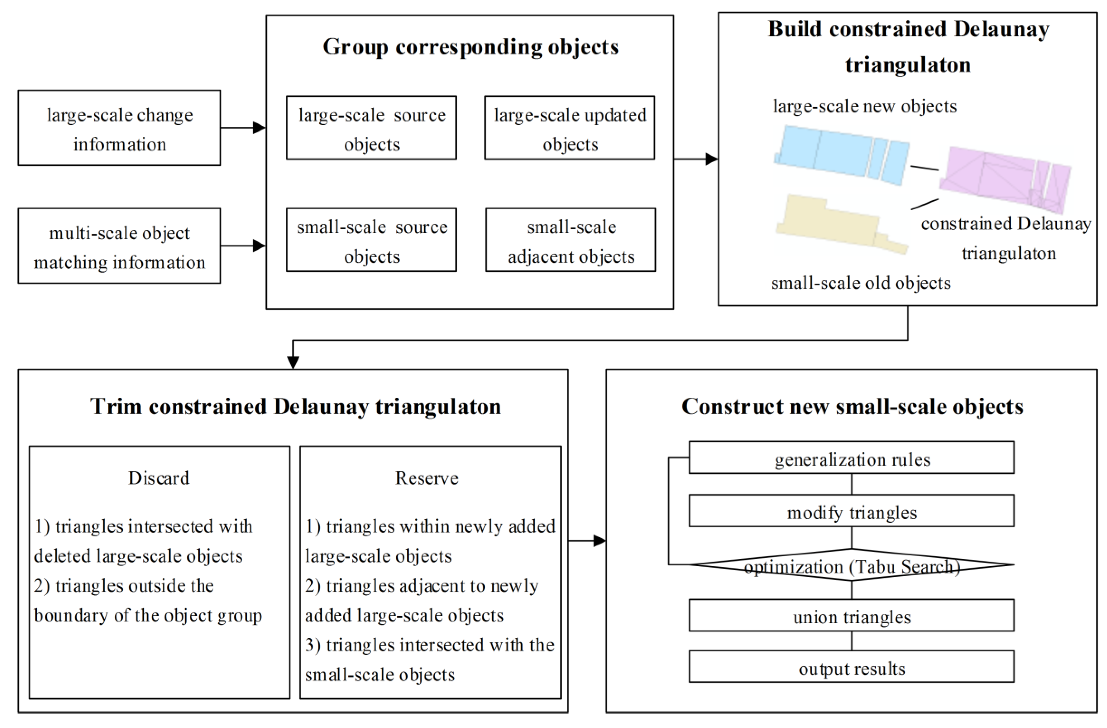
Figure 1 illustrates the main steps in the workflow of our method. We group the corresponding objects at different scales and then decompose the updated objects in the large-scale maps into triangles based on constrained Delaunay triangulation, which are further edited and constructed into objects in the small-scale maps. In essence, we transform the problem of update propagation to the selection and combination of a bunch of tiny triangles, such that the small-scale object can be produced from all corresponding triangles simultaneously to meet the cartographical generalization criteria. Each step is further explained in following sections.

2.2.1. Group Corresponding Objects

To achieve parallel update propagation, spatially-related objects in maps of different scales need to be grouped together for later processing. Considering the types of object updates in the large-scale maps, there are three fundamental operations for update propagation: (1) addition (e.g., new buildings added in the large-scale map have no matching objects in the small-scale map, then based on cartographical generalization rules, objects within a certain distance in both the large- and small-scale maps are grouped); (2) deletion (e.g., buildings removed in the large-scale map have a corresponding object in the small-scale map, then the corresponding small-scale object and its associated large-scale objects are grouped); and (3) modification (e.g., buildings are modified in the large-scale maps in terms of attribute updates or geometric updates, then the corresponding small-scale object and its associated large-scale objects along with large-scale objects within a certain distance are grouped). To simplify the process of update propagation, other types of object updates in the large-scale maps, such as aggregation, partition, exaggeration, and geometric transformation, can be converted to the above-mentioned three types of operations.

2.2.2. Build Constrained Delaunay Triangulation

Large-scale objects are decomposed into groups of triangles based on constrained Delaunay triangulation. The method of constrained Delaunay triangulation is a computational process that breaks polygons into certain segments and forces these segments into triangles [25]. Constrained Delaunay triangulation is widely used in Geographic Information System (GIS) applications [26,27,28] and is embedded in common GIS software (e.g., the ArcGIS software). One key in building constrained Delaunay triangulation is to determine the vertex of each triangle, such that the point sets of vertex could maximize the smallest interior angle of all triangles. 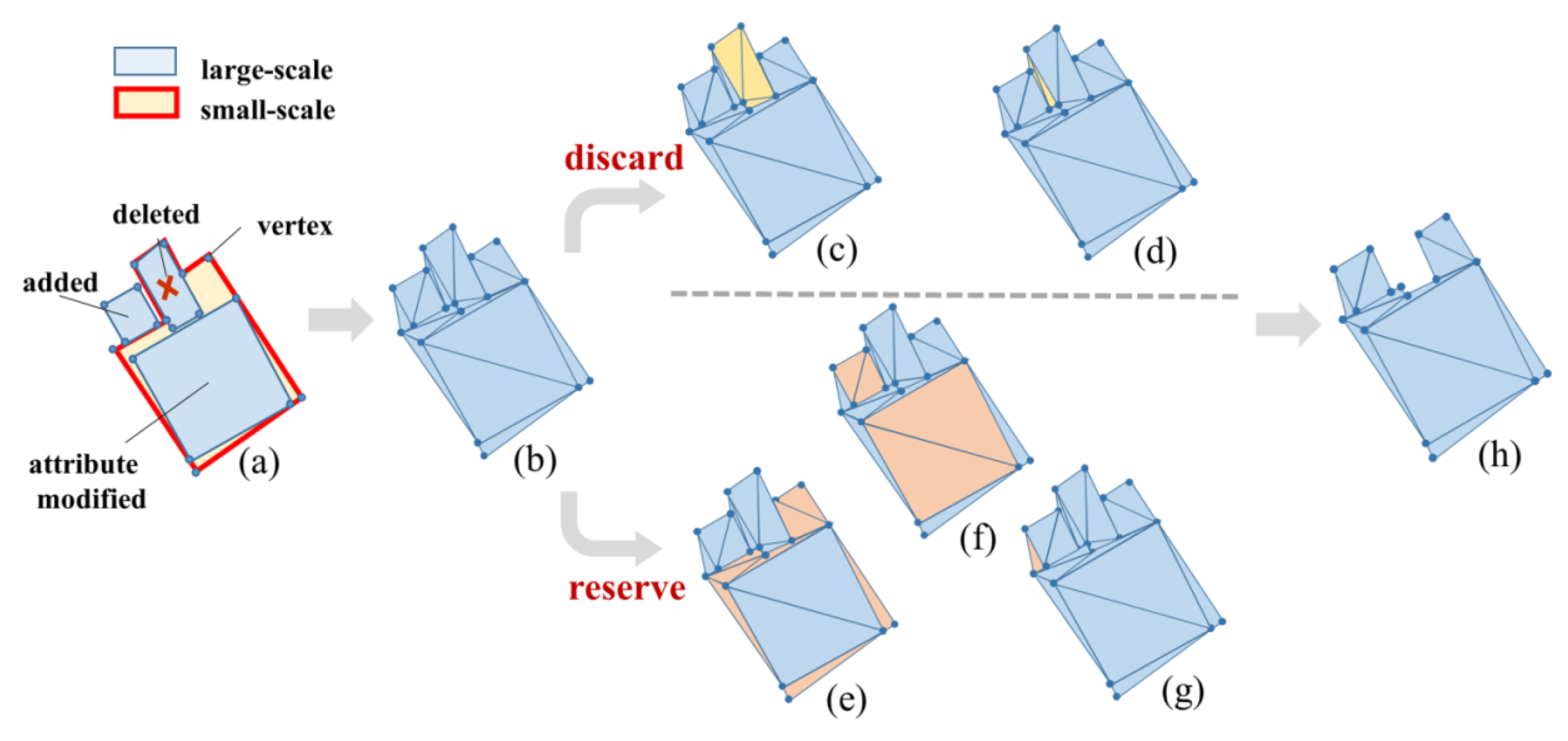We traverse each individual object within the groups of objects, and extract the vertex of each object as the nodes of the triangulation (Figure 2). In addition, because it is necessary to maintain the general shape of the objects in update propagation, the sides of the original polygons are used as conditional boundaries to constrain the extraction of the vertex when building a constrained Delaunay triangulation.

2.2.3. Trim Constrained Delaunay Triangulation

To propagate updates of objects from large- to small-scale maps, we need to fuse the built network of triangles, where the key is to select triangles properly. Accounting for the spatial relationship between updated objects and to-be-updated objects, the rules to operate the triangles are simple: (1) we discard triangles that are intersected with the deleted large-scale objects or triangles that are outside the boundary of the object group and are adjacent to the deleted object; and (2) we reserve triangles that are within the newly added large-scale objects, triangles that are adjacent to the newly added large-scale object, and triangles that are located within the unchanged small-scale object. Figure 2 illustrates the operations on the built network of triangles.

2.2.4. Construct New Small-Scale Objects Using the Tabu Search Algorithm

Consider a trimmed network of constrained Delaunay triangulation as follows:

$$\mathrm{T}=\left[t_1,t_2,t_3,\cdots ,t_n\right]$$

(1)

where $t_{i = 1:n}$ denotes each triangle element in the network.

The key to constructing small-scale objects is to determine the sequence of triangle combination that satisfies cartographical generalization criteria and achieve the best generalization results (e.g., maintain the general shape of the corresponding objects, sustain minimum changing areas, sustain minimum moves of vertex). Due to the cartographical generalization criteria, the processing of update propagation is far more complicated than simple merging of all remaining triangles, because the outcome of the constructed small-scale objects are dependent on the processing sequences of triangles and the cartographical operations. Reconstructing large-scale objects to produce small-scale objects is essentially a problem of combinatorial optimization.

Here we use the Tabu Search algorithm to process the construction of the small-scale objects. The Tabu Search algorithm could obtain near-optimal solutions to the combinatorial problems [29,30]. It searches for global near-optimal solutions without repeating searches by allowing temporary acceptance of worse solutions to avoid being trapped in a local optimum. In the Tabu Search algorithm, potential solutions are stored in the Tabu list, which are used to avoid repeating searches and to find the acceptable solution. The Tabu Search algorithm has a wide range of applications, such as job-shop scheduling, vehicle routing planning, and design of groundwater remediation systems [31,32,33].

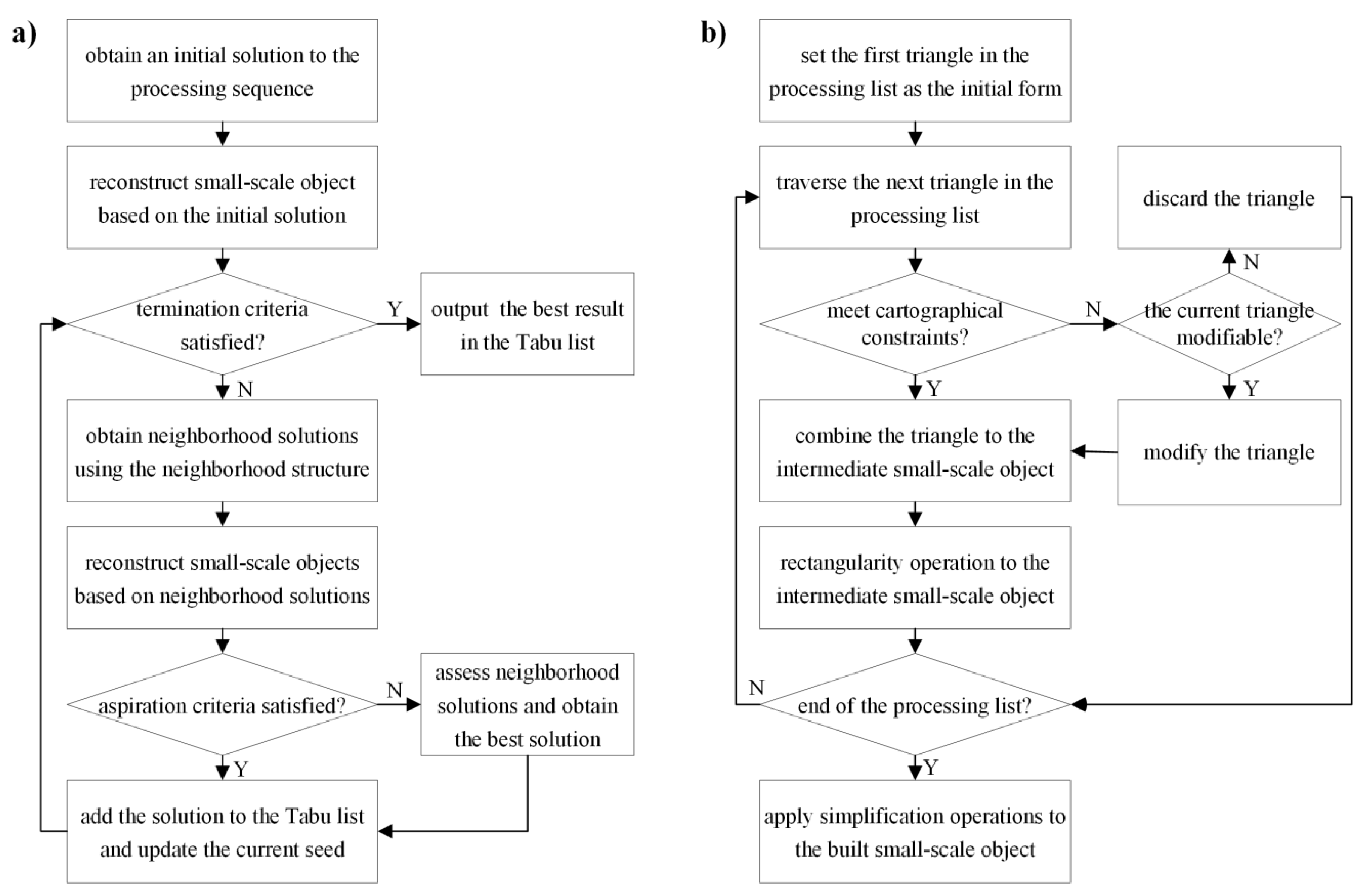
Figure 3a illustrates the procedures to apply the Tabu Search algorithm for constructing the small-scale objects. We first obtain an initial solution to the processing sequence as the current seed and test whether constructed small-scale objects based on the solution satisfy the termination criteria. The iteration processes terminate if the maximum number of iterations is reached or the constructed small-scale objects based on the current seed solution satisfy the mapping criteria (i.e., the constructed small-scale objects fit all cartographical constraints). If the termination criteria are satisfied, the best solution in the Tabu list is chosen as the final output; otherwise, neighborhood solutions to the processing sequence are generated as candidates based on the neighborhood structure of the current seed. If constructed small-scale objects based on one candidate solution could satisfy the aspiration criterion (see the cost function in Section Neighborhood Solutions and Their Evaluation), the solution is added to the Tabu list directly and updated as the current seed; otherwise, the neighborhood solutions are evaluated, whereas the best one is added to the Tabu list and updated as the current seed. The process is repeated iteratively until the termination criteria are satisfied.

2.2.4.1. Initial Solution

To obtain the initial solution to the processing of triangles for generating small-scale objects, it is necessary to build a matrix that is indicative of the adjacent relationships of triangles based on the topological relation as follows:

$$R=\left[\begin{array}{cccc}{R}_{t1,t1}& R_{t1, t2}& \dots & R_{t1,tn}\\ R_{t2,t1}& R_{t2,t2}& \dots & R_{t2,tn}\\ \dots & \dots & R_{ti,tj}& \dots \\ R_{tn,t1}& R_{t2,tn}& \dots & R_{tn,tn}\end{array}\right]$$

(2)

where $t_{i=1:n}$ denotes each triangle element in the network as described in Equation (1), and $R_{ti,tj}$ is a Boolean variable, where $R_{ti,tj}=1$ indicates that $t_i$ and $t_j$ are adjacent and $R_{ti,tj}=0$ indicates that $t_i$ and $t_j$ are not adjacent.

Given the matrix of the adjacent relationships, the initial solution of the processing sequence list can be obtained based on the following steps: (1) A triangle is randomly selected from the constrained Delaunay triangulation as the seed and added to the processing sequence list; (2) If there are neighborhood triangles of the seed element, one neighborhood triangle is randomly chosen as the seed and added to the processing sequence list; otherwise, the first step is repeated; (3) The second step is repeated until all triangles in the constrained Delaunay triangulation are added to the processing sequence list.

2.2.4.2. Construct Small-Scale Objects Based on a Given Solution

To evaluate a given solution to the processing sequence of triangles, it is necessary to construct small-scale objects, of which the process has to account for cartographical generalization rules. Therefore, the construction of small-scale objects can be achieved based on the following steps (Figure 3b): (1) We start from the first element in the processing sequence list; (2) We combine the current polygon with the next triangle in the processing sequence list and check whether the combined polygon violates cartographical constraints; (3) If the cartographical constraints are violated (e.g., an interior angle of the polygon is small), the combined polygon is modified (e.g., the operation of rectangularity) to meet the cartographical constraints. If, even after modification, the combined polygon could not meet the cartographical constraints, the newly added triangle is discarded; (4) Step 2 is repeated until all triangles in the processing sequence list are handled and the small-scale object is built.

There are three operations to meet cartographical constraints during the construction of small-scale objects: (1) Exclusion of unsuitable triangles: unsuitable triangles (e.g., small long narrow triangles connected to the main polygon) are possibly introduced when building or trimming constrained Delaunay triangulation [34]. If the triangle has a very small interior angle and if it does not share a common side with other triangles or it only shares one very short side with other triangles, the corresponding triangle is considered as an unsuitable triangle and is excluded during the construction of the small-scale objects; (2) Rectangularity: given a near-rectangular interior angle, rectangularity is to convert the interior angle to a rectangle, which is done by drawing a vertical line from the corresponding vertex that connects to the shorter side to the longer side and regenerating the shape of the polygon; (3) Elimination of small objects: if the object in a topographic map has an area smaller than the minimum representable area, the corresponding object is removed because we do not consider the operation of exaggeration in the current study. An example provided in Figure 4b illustrates the application of the operations when constructing the small-scale objects.

2.2.4.3. Neighborhood Solutions and Their Evaluation

If the constructed small-scale objects does not satisfy the mapping criteria, a neighborhood solution is generated based on the neighborhood structure Equation (2), which is derived based on the spatial relationship of the triangles. First, each adjacent triangle of the first element in the current processing sequence list is set as the first element of the new processing sequence list. If there are no adjacent triangles of the first element in the current processing sequence list, three random and unsearched triangles are chosen as the first elements of the new processing sequence list. Second, similar to the method that derives the initial solution of the processing sequence list (Section 2.2.4.1.) we start with the given first elements of the processing sequence lists to obtain new solutions as the neighborhood solutions. Last, we evaluate neighborhood solutions that are used to construct small-scale objects and add the optimal solution to the Tabu list.

Evaluating the solutions needs to account for how well the constructed small-scale object meets cartographical constraints and reserves the spatial characteristics of the large-scale objects [35]. Because we have already modified the small-scale objects to meet cartographical constraints when constructing small-scale objects, we use a cost function to evaluate the reservation of the spatial characteristics as follows:

$$I_{cost}=w_1{I}_{as}+w_2{I}_{ps}+w_3{I}_{ss}$$

(3)

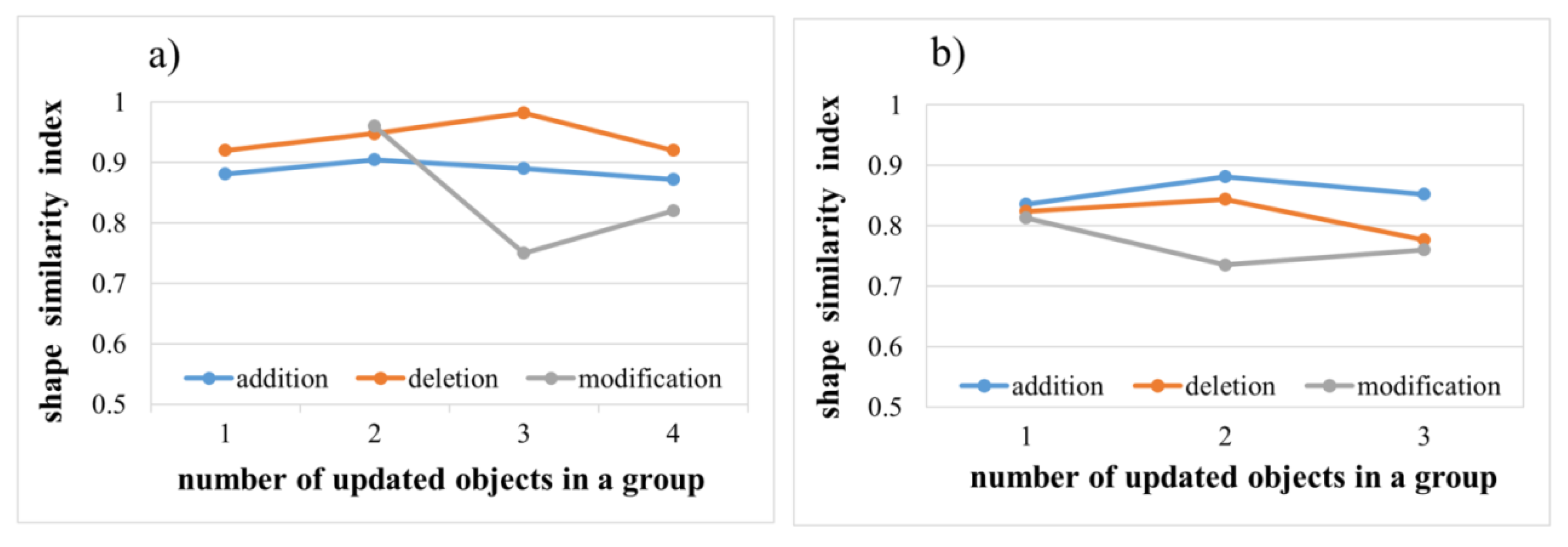
where $I_{cost}$ is the overall cost function; $I_{as}$, $I_{ps}$, and $I_{ss}$ represent the area similarity index, the position similarity index, and the shape similarity index, respectively; and $w_1$, $w_2$, and $w_3$ are weighting functions. When performing the evaluation in our study, all weights have a value of 1/3.

The components in the cost functions are derived as follows:

$$I_{as}=1-\frac{\left|A_s-A_l\right|}{\max \left(A_s,A_l\right)}$$

(4)

$$I_{ps}=1-\frac{\sqrt{{(X_s-X_l)}^2+{(Y_s-Y_l)}^2}}{\sqrt{\max {\left(X_s,X_l\right)}^2+\max {\left(Y_s,Y_l\right)}^2}}$$

(5)

$$I_{ss}=\frac{A_o}{\max \left(A_s,A_l\right)}$$

(6)

where $A_s$ and $A_l$ are the areas of corresponding small- and large-scale objects, respectively; $X_s$ and $X_l$ are the horizontal coordinates of the centroid point of the small- and large-scale objects, respectively; $Y_s$ and $Y_l$ are the vertical coordinate of the centroid point of the small- and large-scale objects, respectively; $A_{Lt}$ and $A_{St}$ are the total areas of corresponding objects in the large- and small-scale maps, respectively; and $A_o$ is the overlapping area between the small- and large-scale objects. All indices have the value between 0 and 1, thus the value of the overall cost function $I_{cost}$ ranges from 0 to 1.

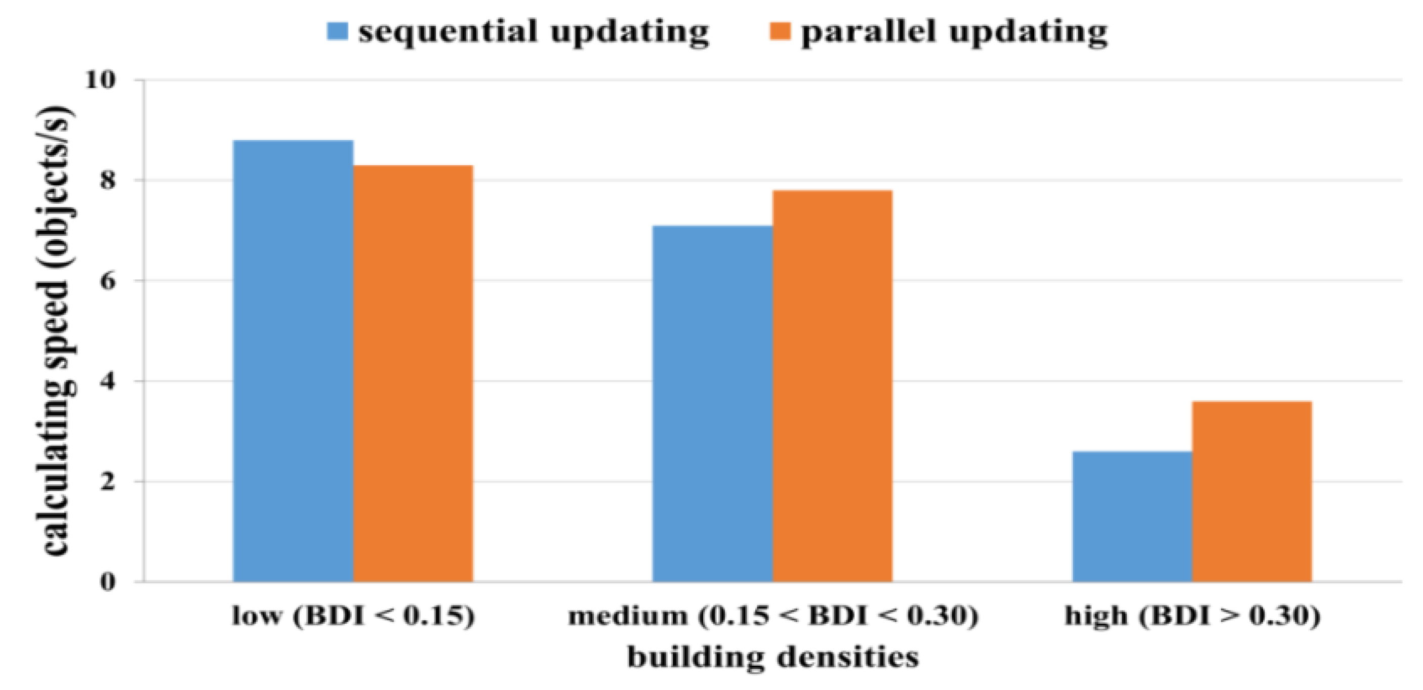
2.2.5. Parallel versus Sequential Updating

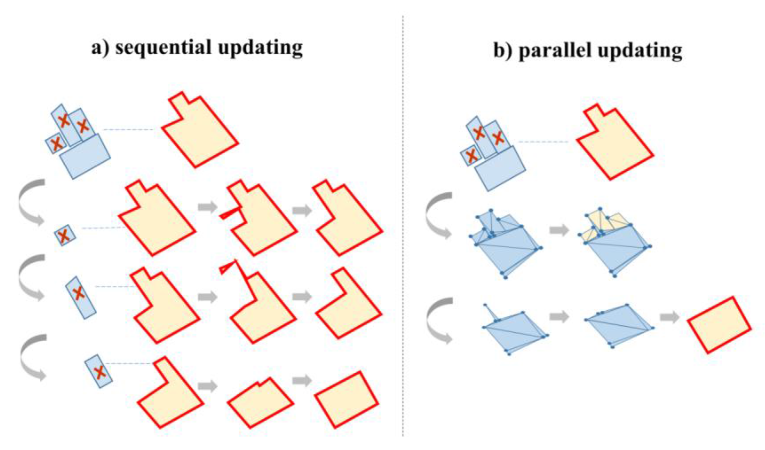
The method that we developed essentially supports parallel processing of updated residential areas to produce small-scale objects, and is different from the sequential processing method. Figure 4 shows an example that illustrates the difference between parallel and sequential processing in constructing small-scale objects. The sequential method chooses to traverse all updated large-scale objects sequentially and propagate them to the small-scale objects [8,36]. For the m:1 object-matching relationship, the sequential method neglects the mutual connections among adjacent large-scale objects and propagates the updates one by one, thus resulting in a heavy computational burden. In comparison, our method groups large-scale objects and operates all decomposed triangles together, thereby potentially improving the computational efficiency.

2.3. Case Study and Materials

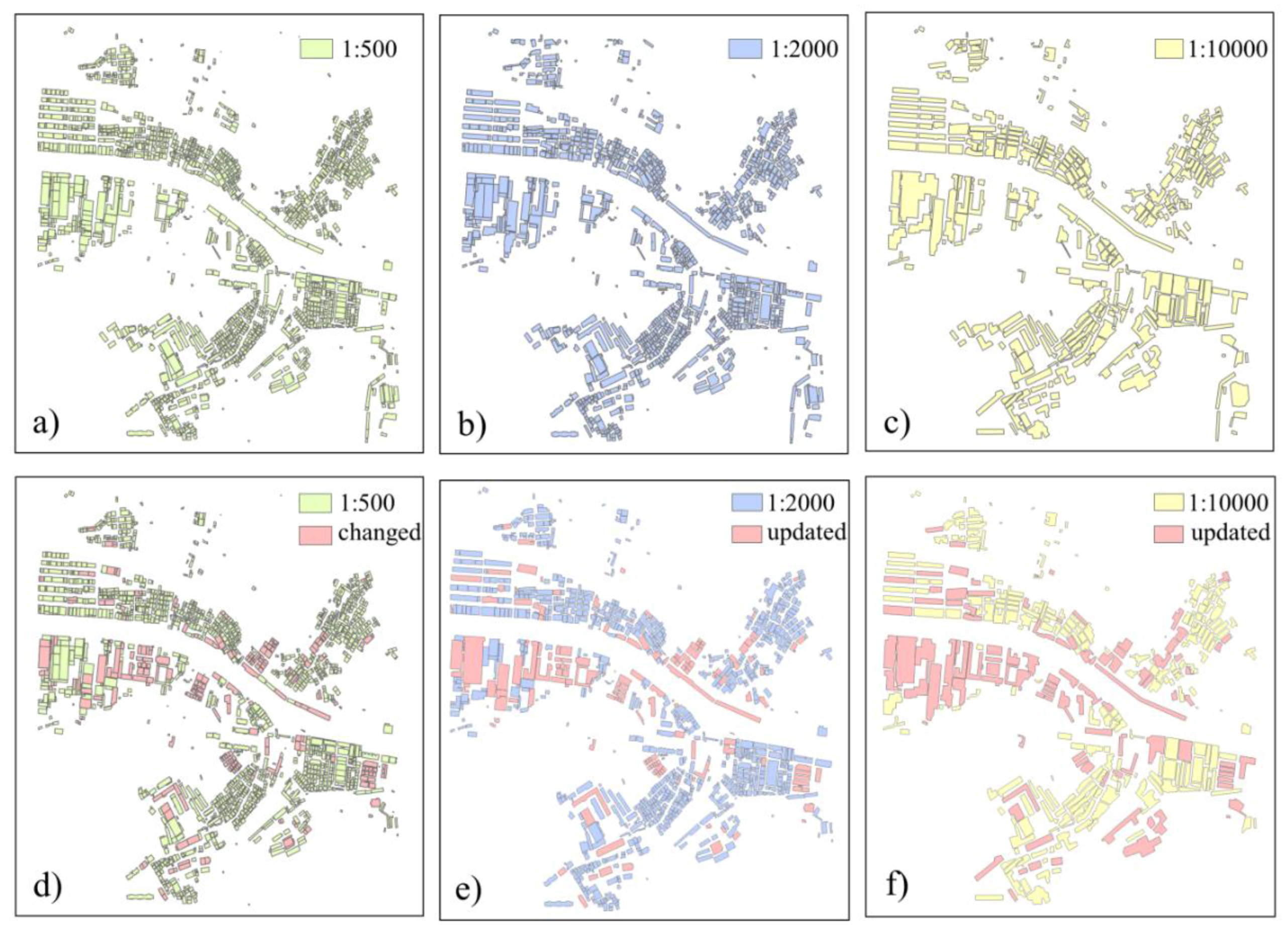
We applied our method to update the digital maps of residential areas in the Zengcheng city in south China. The digital maps shown in Figure 5 were obtained from local Administration of Surveying Mapping and Geo-Information, and were provided for three different scales (i.e., 1:500, 1:2000, and 1:10,000). All original maps were produced for the year of 2005 (Figure 5a–c). The 1:500 map was updated for the year of 2013 (Figure 5d) and the 1:2000 and 1:10,000 topographical maps were maps to be updated. To evaluate the obtained results, the 1:2000 and 1:10,000 topographic maps (Figure 5e,f, respectively) were also manually updated by professionals based on the updated 1:500 topographic map.

The produced small-scale maps have to meet cartographic constraints. Referring to the regulations of cartographic symbols for national fundamental scale maps in China, the maximum distance for aggregation is set as 1 and 2 m for the 1:2000 and 1:10,000 topographic maps, respectively; the tolerance of data error in the map is set as 1 and 1.5 m for the 1:2000 and 1:10,000 topographic maps, respectively; and the minimum representable area in the map is set as 24 and 48 square meters for the 1:2000 and 1:10,000 topographic maps, respectively.

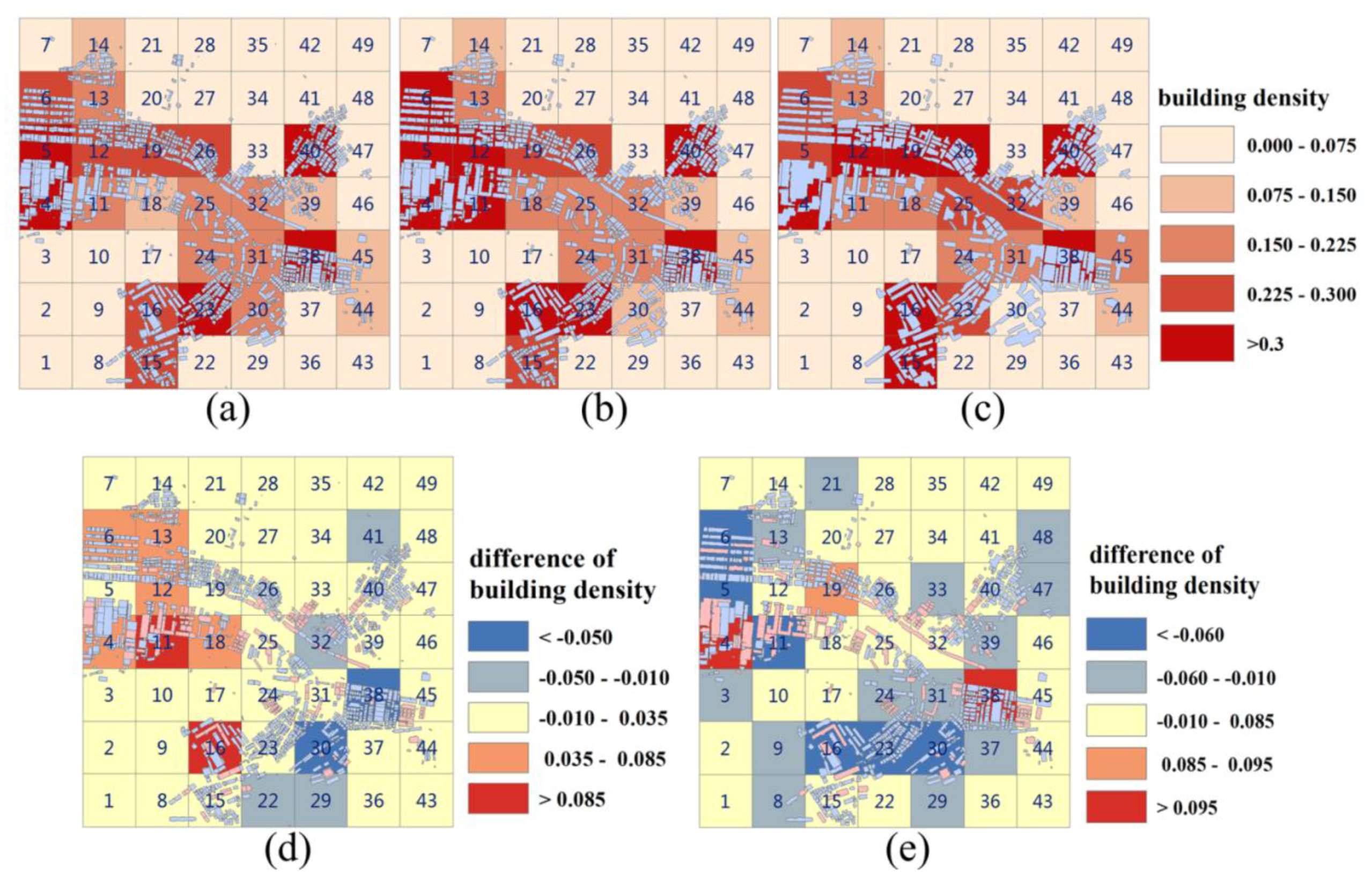
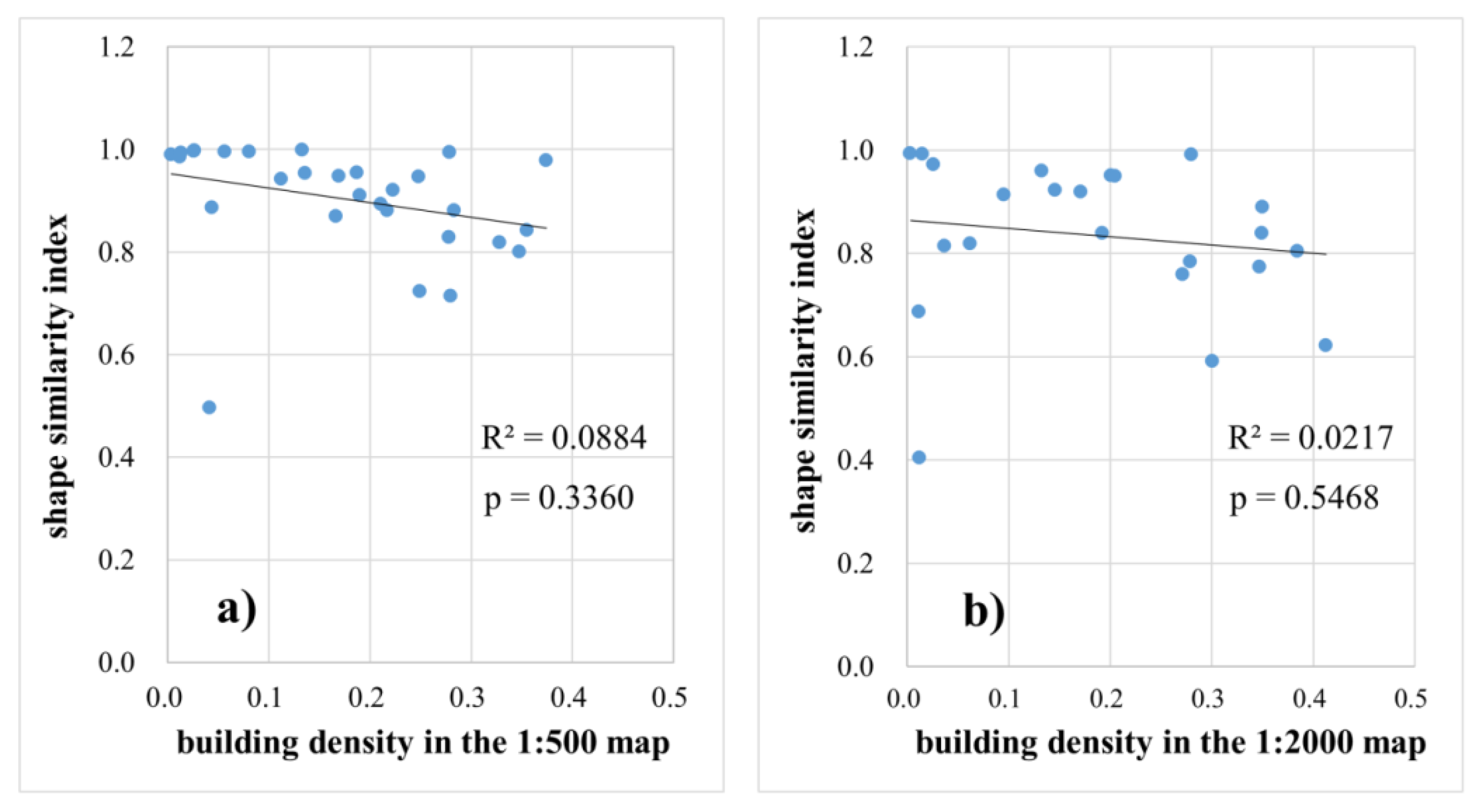
In addition, to understand how the method of update propagation would influence the spatial pattern of residential areas in maps of different scales, the building density index is used in our case study and is derived as follows:

$$I_{BD}=\frac{{{\displaystyle \sum }}^{\text{}}{A}_i}{A_{grid}}$$

(7)

where $I_{BD}$ is the building density index, $A_i$ is the area of each polygon of the residential area located in a given grid, and $A_{grid}$ is the total area of a grid.

3. Results and Discussion

3.1. Accuracy Analysis

Figure 6 shows the updated topographic maps at the scales of 1:2000 and 1:10,000. The spatial patterns of our updated topographic maps at different scales match that produced at the scale of 1:500.

Table 1. Statistical analysis of the updated small-scale maps for different object-matching relationships as compared with the corresponding large-scale topographic maps.

Update Propagation	Object-Matching	Mean Position Similarity	Mean Area Similarity	Mean Shape Similarity
1:500 to 1:2000	1:1	0.999	0.998	0.998
	m:1	0.999	0.871	0.879
	m:n	0.999	0.900	0.898
1:2000 to 1:10,000	1:1	0.999	0.859	0.859
	m:1	0.998	0.685	0.805
	m:n	0.998	0.867	0.842

shows statistical results for updates of residential areas among different scales. The mean values of the position similarity index, the area similarity index, and the shape similarity index are almost all more than 0.80, indicating that the geometric characteristics of large-scale objects are retained well in the update processing. The mean values of the position similarity index are all higher than 0.99, suggesting that the offsets of the centroid points between large- and small-scale objects are quite small. The changes of polygon areas and polygon shapes among objects at different scales are dependent on the scale factor, the object-matching relationship and the cartographical operations. For example, the 1:1 object-matching relationship has higher values of area similarity index than other object-matching relationships, largely because gaps between updated large-scale objects are filled in the small-scale map when constructing small-scale objects for the m:1 or m:n object-matching relationships. Similarly, objects with the m:1 object-matching relationship have lower values of area similarity and shape similarity than others, because building polygons are often merged when updating the small-scale maps. Such effects are shown to be strong when updating the 1:10,000 topographic map, resulting in relatively low values of area similarity and shape similarity.

The shape similarity index is further studied to understand the influence of the number of objects that are grouped on the updating of the large-scale maps (Figure 7). Generally, the values of the shape similarity index are higher when updating the 1:2000 topographic maps than when updating the 1:10,000 topographic maps, mainly because the influence of cartographical generalization on update propagation is stronger when updating smaller-scale maps. The shape similarity index is consistently high but decreases slightly as the updated object numbers increase because the more large-scale objects are updated, the more geometric modifications likely occur when constructing small-scale objects. The modification operation has to deal with both newly added and newly deleted objects, and thus likely has more mapping uncertainties and leads to lower values of shape similarity than the operations of addition and deletion.

When updating the 1:2000 topographic maps, the deletion operation results in higher shape similarity than the addition operation. One reason is that some of the added objects in the 1:500 topographic maps violate the cartographical rule of minimum representable area. If these newly added polygons have no adjacent objects to combine for producing small-scale objects, they are not included in the 1:2000 topographic maps, thus resulting in decreased values of the shape similarity index. For the operation of deletion, most propagated updates are used to modify small-scale objects and thus only have slight impacts on the shape similarity index. The operation of modification often involves complex processing of updates, and thus results in relatively lower values of the shape similarity index. When updating the 1:10,000 topographic maps, only a few objects violate the cartographical rule of the minimum representable area, and the operation of addition gives higher values of the shape similarity index than the other operations.

In addition to the above accuracy assessment by making comparisons between the large-scale maps and the updated small-scale maps,

Table 2. Statistical analysis of the updated maps for different object-matching relationships as compared with manually updated topographic maps.

Updated Maps	Object-Matching	Mean Position Similarity	Mean Area Similarity	Mean Shape Similarity
1:2000	1:1	0.999	0.985	0.984
	m:1	0.999	0.971	0.975
	m:n	0.999	0.976	0.978
1:10,000	1:1	0.999	0.975	0.970
	m:1	0.999	0.908	0.895
	m:n	0.999	0.917	0.906

summarizes the statistical results for the comparisons between the algorithm-updated maps and the manually updated maps at the same scale. Most of the values are as high as above 0.90 in Table 2 and nearly all values in Table 2 are higher than in Table 1, mainly because the map scales are matched when conducting the statistical analysis. The pattern shown in Table 2 is similar to that shown in Table 1. For example, the m:1 object-matching relationships gives the lowest values of area similarity and shape similarity, largely due to the aggregation operation of multiple building polygons. These results suggest that our method is able to provide accurate updates of topographic maps as evaluated against manually updated maps.

3.2. The Spatial Pattern of Building Densities

Figure 8 shows the building densities in the updated topographic maps to help understand the influences of updating residential areas. The maps that are classified into 7-by-7 regular grid cells are shown to have differences of building densities among topographic maps of different scales. The reason is largely due to the multi-scale representations of entities and cartographical generalization such as aggregation of adjacent objects and deletion of small objects. Grids with large differences in building densities mainly coincide with areas of high building densities such as grid 16 and 38.

Table 3. Statistical summaries for building densities in the updated maps.

Building Density Index	Number of Grids (1:500)	Number of Grids (1:2000)	Number of Grids (1:10,000)
0.000–0.075	26	26	27
0.075–0.150	5	5	3
0.150–0.225	7	6	6
0.225–0.300	6	8	5
>0.300	5	4	8

lists the numbers of grid cells for different building densities. The number of grid cells in each class only has slight differences, indicating that propagated updates effectively maintain building densities in the topographic maps of different scales and generally keep the spatial patterns of residential area. For most of the cases, the number of grids in the small-scale map increases for areas with high building densities, mainly because many blank areas in-between adjacent objects in the large-scale map are filled up in the small-scale map due to the aggregation operation.

Figure 9 shows the relationship between the shape similarity indexes of the updated objects and building densities. The shape similarity index appears to decrease as the building densities increase when updating the 1:2000 and 1:10,000 topographic maps. The influences of cartographic operations are stronger in areas with high building densities than in areas with low building densities, resulting in a relatively low shape similarity index in areas with high building densities. When conducting simple correlation analysis between the shape similarity indexes and building densities, the correlation coefficient is insignificant as denoted by the p values, though the shape similarity index has a small decreasing trend, indicating that propagated updates effectively maintained the shapes of updated objects for varied building densities in topographic maps of different scales.

3.3. Comparisons between Sequential and Parallel Updating

Comparisons between the sequential and parallel updating methods are shown in Figure 10 to help understand their differences in computational efficiency, as measured by the metric of average updated object numbers per second. In areas with low building densities (${\mathrm{I}}_{\text{BD}}<0.15$), the sequential updating method appears to be faster than the parallel updating method. One reason is that areas of low building densities have sparse polygons of updated residential areas and many 1:1 object-matching relationships. It is relatively easy to operate individual object updates sequentially, but it could take time to analyze the triangle networks in our proposed parallel method. Because there are more m:1 object-matching relationships in areas with medium ($0.15<{\mathrm{I}}_{\text{BD}}<0.30$) and high (${\mathrm{I}}_{\text{BD}}>0.30$) building densities, the parallel updating method could effectively reduce the computation burden. In areas with high building densities, the parallel updating method is shown to increase the computational speed by 27.8%. We did not compare our method with other sophisticated methods, due to difficulties in obtaining their source code.

4. Conclusions

To update residential areas in multi-representation databases, we propose a new method to propagate updates of large-scale objects to produce small-scale objects. The method decomposes large-scale objects into triangles based on constrained Delaunay triangulation. The Tabu Search algorithm is applied to find the solutions to combine triangles and construct small-scale objects that satisfy cartographical constrains. We applied the developed method to update topographic maps and found that the updated small-scale maps have similar patterns to the large-scale maps in terms of vertex displacement, area changes, and morphological changes. Because the method operates on triangles together and allows for parallel processing of update propagation, it acts more effectively in areas with high building densities than the method that operates objects sequentially. The method, though it requires further tests on other locations, shows promise to update residential areas in multi-representation databases.

References

1. Goodchild, M.F. Citizens as voluntary sensors: Spatial data infrastructure in the world of web 2.0. Int. J. Spat. Data Infrastruct. Res. 2007, 2, 24–32. [Google Scholar]
2. Xiong, Y.; Huang, S.; Chen, F.; Ye, H.; Wang, C.; Zhu, C. The impacts of rapid urbanization on the thermal environment: A remote sensing study of Guangzhou, South China. Remote Sens. 2012, 4, 2033–2056. [Google Scholar] [CrossRef]
3. Zhang, X.; Kang, T.; Wang, H.; Sun, Y. Analysis on spatial structure of landuse change based on remote sensing and geographical information system. Int. J. Appl. Earth Obs. Geoinf. 2010, 12, S145–S150. [Google Scholar] [CrossRef]
4. Shalaby, A.; Tateishi, R. Remote sensing and GIS for mapping and monitoring land cover and land-use changes in the Northwestern coastal zone of Egypt. Appl. Geogr. 2007, 27, 28–41. [Google Scholar] [CrossRef]
5. Bocco, G.; Mendoza, M.; Velázquez, A. Remote sensing and GIS-based regional geomorphological mapping—A tool for land use planning in developing countries. Geomorphology 2001, 39, 211–219. [Google Scholar] [CrossRef]
6. Kilpeläinen, T. Maintenance of multiple representation databases for topographic data. Cartogr. J. 2000, 37, 101–107. [Google Scholar] [CrossRef]
7. Zhou, S.; Jones, C.B. A multi-representation spatial data model. In Advances in Spatial and Temporal Databases; Springer: Heidelberg, Germany, 2003; pp. 394–411. [Google Scholar]
8. Bobzien, M.; Burghardt, D.; Petzold, I. Re-generalisation and construction—Two alternative approaches to automated incremental updating in MRDB. In Proceedings of the 22nd International Cartographic Conference, La Coruña, Spain, 9–16 July 2005.
9. Harrie, L.; Hellström, A.-K. A prototype system for propagating updates between cartographic data sets. Cartogr. J. 1999, 36, 133–140. [Google Scholar] [CrossRef]
10. Baltsavias, E.; Zhang, C. Automated updating of road databases from aerial images. Int. J. Appl. Earth Obs. Geoinf. 2005, 6, 199–213. [Google Scholar] [CrossRef]
11. Guo, T.; Zhang, X.; Liang, Z. Research on change information recognition method of vector data based on neural network decision tree. Acta Geod. Cartogr. Sin. 2013, 42, 937–943. [Google Scholar]
12. Fan, Y.; Yang, J.; Zhang, C.; Zhu, D. A event-based change detection method of cadastral database incremental updating. Math. Comput. Model. 2010, 51, 1343–1350. [Google Scholar] [CrossRef]
13. Anders, K.-H.; Sester, M.; Bobrich, J. Incremental update in an MRDB. In Proceedings of the 23rd International Cartographic Conference, Moscow, Russia, 4–10 August 2007.
14. Bobzien, M.; Burghardt, D.; Petzold, I.; Neun, M.; Weibel, R. Multi-representation databases with explicitly modeled horizontal, vertical, and update relations. Cartogr. Geogr. Inf. Sci. 2008, 35, 3–16. [Google Scholar] [CrossRef]
15. Qi, H.; Li, Z.; Chen, J. Automated change detection for updating settlements at smaller-scale maps from updated larger-scale maps. J. Spat. Sci. 2010, 55, 133–146. [Google Scholar] [CrossRef]
16. Lin, Y.; Liu, W.-Z.; Chen, J. Modeling spatial database incremental updating based on base state with amendments. Procedia Earth Planet. Sci. 2009, 1, 1173–1179. [Google Scholar] [CrossRef]
17. Chen, J.; Lin, Y.; Liu, W. Formal classification of spatial incremental changes for updating. Acta Geod. Cartogr. Sin. 2012, 41, 108–114. [Google Scholar]
18. Zhang, X.; Guo, T.; Tang, T. An adaptive method for incremental updating of vector data. Acta Geod. Cartogr. Sin. 2012, 41, 613–619. [Google Scholar]
19. Foerster, T.; Stoter, J.; Kobben, B. Towards a formal classification of generalization operators. In Proceedings of the 23rd International Cartographic Conference, Moscow, Russia, 4–10 August 2007.
20. Revell, P.; Antoine, B. Automated matching of building features of differing levels of detail: A case study. In Proceedings of the 24th International Cartographic Conference, Santiago de Chile, Chile, 15 November 2009.
21. Walter, V.; Fritsch, D. Matching spatial data sets: A statistical approach. Int. J. Geogr. Inf. Sci. 1999, 13, 445–473. [Google Scholar] [CrossRef]
22. Junkui, X.U.; Fang, W.U.; Qian, H. The establishment and usage of the neighborhood scale settlement features’ links in spatial data updating process. Acta Geod. Cartogr. Sin. 2013, 42, 898–905. [Google Scholar]
23. Zhou, S.; Regnauld, N.; Roensdorf, C. Generalisation log for managing and utilising a multi-representation spatial database in map production. Comput. Environ. Urban Syst. 2009, 33, 334–348. [Google Scholar] [CrossRef]
24. Dilo, A.; van Oosterom, P.; Hofman, A. Constrained tGAP for generalization between scales: The case of Dutch topographic data. Comput. Environ. Urban Syst. 2009, 33, 388–402. [Google Scholar] [CrossRef]
25. Chew, L.P. Constrained delaunay triangulations. Algorithmica 1989, 4, 97–108. [Google Scholar] [CrossRef]
26. Tortosa, L.; Vicent, J.-F.; Zamora, A. A model to simplify 2D triangle meshes with irregular shapes. Appl. Math. Comput. 2010, 216, 2937–2946. [Google Scholar] [CrossRef]
27. Liu, S.; Hu, X.; Xi, Y.; Liu, T. 2D inverse modeling for potential fields on rugged observation surface using constrained Delaunay triangulation. Comput. Geosci. 2015, 76, 18–30. [Google Scholar] [CrossRef]
28. Ai, T.; Guo, R. Extracting center-lines and building street network based on constrained Delaunay triangulation. Acta Geod. Cartogr. Sin. 2000, 29, 348–354. [Google Scholar]
29. Glover, F. Tabu search-part I. ORSA J. Comput. 1989, 1, 190–206. [Google Scholar] [CrossRef]
30. Glover, F. Tabu search-part II. ORSA J. Comput. 1990, 2, 4–32. [Google Scholar] [CrossRef]
31. Yang, Y.; Wu, J.; Sun, X.; Wu, J.; Zheng, C. A niched Pareto Tabu search for multi-objective optimal design of groundwater remediation systems. J. Hydrol. 2013, 490, 56–73. [Google Scholar] [CrossRef]
32. Krichen, S.; Faiz, S.; Tlili, T.; Tej, K. Tabu-based GIS for solving the vehicle routing problem. Exp. Syst. Appl. 2014, 41, 6483–6493. [Google Scholar] [CrossRef]
33. Palacios, J.J.; González, M.A.; Vela, C.R.; González-Rodríguez, I.; Puente, J. Genetic Tabu search for the fuzzy flexible job shop problem. Comput. Oper. Res. 2015, 54, 74–89. [Google Scholar] [CrossRef]
34. Gao, Z.; Yu, Z.; Holst, M. Quality tetrahedral mesh smoothing via boundary-optimized Delaunay triangulation. Comput. Aided Geom. Des. 2012, 29, 707–721. [Google Scholar] [CrossRef] [PubMed]
35. Harrie, L.; Stigmar, H. An evaluation of measures for quantifying map information. ISPRS J. Photogramm. Remote Sens. 2010, 65, 266–274. [Google Scholar] [CrossRef]
36. Wang, Y.; Du, Q.; Ren, F.; Zhao, Z. A propagating update method of multi-represented vector map data based on spatial objective similarity and unified geographic entity code. In Cartography from Pole to Pole; Springer: Berlin, Germany, 2014; pp. 139–153. [Google Scholar]
Figure 1. The workflow to propagate the updates of residential areas in multi-representation databases.
Ijgi 05 00080 g001
Figure 2. Examples of the processing of constrained Delaunay triangulation are shown for (a) the group of corresponding objects and extracted vertex; (b) built constrained Delaunay triangulation; (c) discarded triangles intersected with the deleted object; (d) discarded triangles that are outside the boundary of the object group and are adjacent to the deleted object; (e) reserved triangles that are located within the unchanged part of the small-scale object; (f) reserved triangles that are located within the newly added or modified large-scale object; (g) reserved triangles that are adjacent to the newly added large-scale object; and (h) trimmed constrained Delaunay triangulation.
Ijgi 05 00080 g002
Figure 3. The flow diagrams are shown for (a) the Tabu Search algorithm to find an optimal solution; and (b) construction of the small-scale object based on a given solution.
Ijgi 05 00080 g003
Figure 4. Examples are shown to compare (a) the sequential updating strategy; with (b) the parallel updating strategy.
Ijgi 05 00080 g004
Figure 5. The study materials are shown for (a) the 1:500 topographic map; (b) the 1:2000 topographic map; (c) the 1:10,000 topographic map; (d) the updated 1:500 topographic map; (e) the updated 1:2000 topographic map; and (f) the updated 1:10,000 topographic map.
Ijgi 05 00080 g005
Figure 6. The updated maps are shown for (a) the 1:2000 topographic map; and (b) the 1:10,000 topographic map.
Ijgi 05 00080 g006
Figure 7. Analysis between the number of updated objects in a group and shape similarity index is shown for (a) propagating updates from the 1:500 map to the 1:2000 map; and (b) propagating updates from the 1:2000 map to the 1:10,000 map.
Ijgi 05 00080 g007
Figure 8. Analysis of building densities among multi-scales updated maps is shown for (a) building densities of the 1:500 map; (b) building densities of the 1:2000 map; (c) building densities of the 1:10,000 map; (d) the differences in building densities between the 1:500 map and the 1:2000 map; and (e) the differences in building densities between the 1:2000 map and the 1:10,000 map.
Ijgi 05 00080 g008
Figure 9. The relationships between shape similarity index and building densities are shown for (a) propagated updates from the 1:500 topographic map to the 1:2000 topographic map; and (b) propagated updates from the 1:2000 topographic map to the 1:10,000 topographic map. The displayed points were obtained from grid cells in Figure 8.
Ijgi 05 00080 g009
Figure 10. Comparison of calculation speed between the sequential and parallel updating methods. BDI denotes building density index as described in Equation (7).
Ijgi 05 00080 g010