A Novel Absolute Orientation Method Using Local Similarities Representation

Abstract

Absolute orientation is an important method in the field of photogrammetry. The technique is used to transform points between a local coordinate reference system and a global (geodetic) reference system. The classical transformation method uses a single set of similarity transformation parameters. However, the root mean square error (RMSE) of the classical method is large, especially for large-scale aerial photogrammetry analyses in which the points used are triangulated through free-net bundle adjustment. To improve the transformation accuracy, this study proposes a novel absolute orientation method in which the transformation uses various sets of local similarities. A Triangular Irregular Network (TIN) model is applied to divide the Ground Control Points (GCPs) into numerous triangles. Local similarities can then be computed using the three vertices of each triangle. These local similarities are combined to formulate the new transformation based on a weighting function. Both simulated and real data sets were used to assess the accuracy of the proposed method. The proposed method yields significantly improved plane and z-direction transformed point accuracies compared with the classical method. On a real data set with a mapping scale of 1:30,000 for a 53 km × 35 km study area, the plane and z RMSEs can be reduced from 1.2 m and 12.4 m to 0.4 m and 3.2 m, respectively.

1. Introduction

Absolute orientation is a fundamental procedure in the field of photogrammetry and plays a crucial role in the transformation of three-dimensional (3D) points from a local to a global (geodetic) coordinate reference system. The technique has been widely used in numerous applications, such as the construction of 3D city models using multi-view stereo mobile mapping systems [1,2,3], the generation of 3D maps [4,5], the reconstruction of buildings [6,7,8,9] and 3D human models, and the manufacture of 3D physical models of large statues [10,11].

The classical absolute orientation method accurately represents the geometric relationships between 3D points in the local and global coordinate reference systems by means of a similarity transformation, which consists of one scaling parameter, three rotation angles and three translation vector parameters [12]. The problem to be solved can be defined as a non-linear least-squares problem based on these seven unknown parameters for three or more pairs of 3D points in two coordinate reference systems. The solution can be obtained via a non-linear optimization method, in which the optimal values in the unknown variable space can be acquired through sequential iteration from some initial conditions. Blostein et al. [13] studied the global minima of this non-linear optimization problem using an iterative solution method to yield precise estimations. Although the iterative method can produce accurate estimations, the transformation parameters require initialization. In addition, divergence may occur if the Hessian matrix is singular. Many studies have focused on obtaining a closed-form solution without initialization. Horn et al. [14] proposed a closed-form absolute orientation solution using orthonormal matrices. However, this algorithm often produces an incorrect rotation matrix. Aurn et al. [15] solved this problem by utilizing another closed-form method based on singular value decomposition (SVD) to stably determine the transformation parameters.

In these previous methods, a single similarity transformation with a single set of seven parameters was used to represent the relationships between objects in two coordinate reference systems, as applied to aerial photogrammetry. However, if the study area is sufficiently large, these methods produce inaccurate point transformations. These inaccuracies arise primarily because point transformations with large deformation in a large-scale study case cannot satisfy the requirements of rigid-body transformation, as represented by the single set of seven similarity transformation parameters used in the classical method. Therefore, it is infeasible to accurately represent the transformation of two such point sets using a single similarity transformation of this type, and thus, a larger root mean square error (RMSE) is incurred. This study proposes a new transformation method that combines various local similarities rather than relying on a single similarity transformation. A local similarity refers to a set of similarity transformations computed using three pairs of 3D points in a local region. A Triangular Irregular Network (TIN) model is used to divide the given pairs of 3D points into various triangles. Local similarities can then be calculated using the three vertices of each triangle. The new transformation is expressed in terms of the local similarities calculated from all triangles. These similarities are combined by means of a weighted power function.

This paper is organized as follows. Section 2 briefly introduces the classical absolute orientation method based on a single similarity transformation. Section 3 introduces the proposed novel absolute orientation method based on local similarities. The performance of the proposed method is demonstrated using six simulated data sets and a real data set in Section 4. Section 5 presents the conclusions.

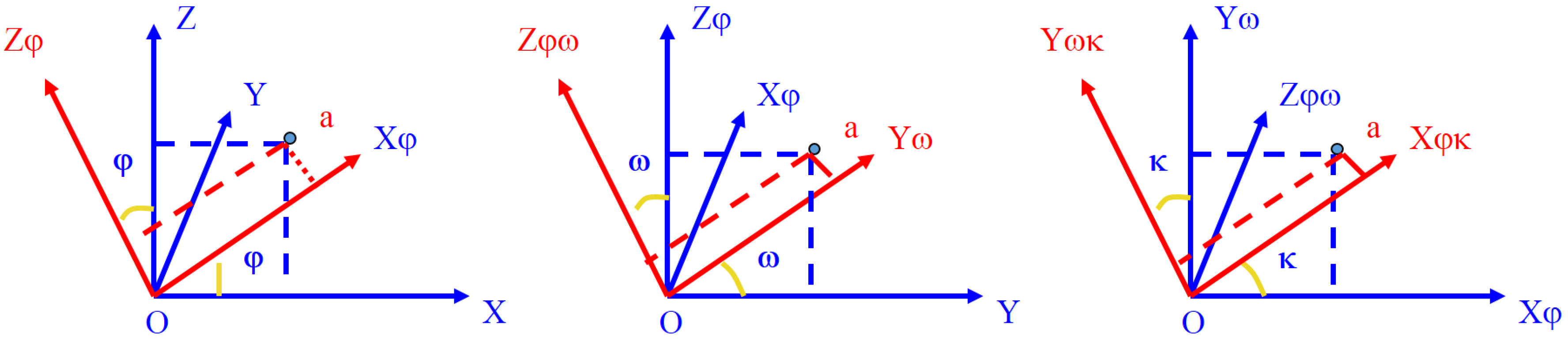
2. Single Similarity Transformation

The classical absolute orientation method searches for the optimal rigid-body transformation to perform a 3D point transformation from a local to a global coordinate reference system. This process is commonly expressed in terms of a similarity transformation with only seven degrees of freedom. A single set of similarity transformation parameters is estimated to transform points from the local to the global coordinate system. The classical method is also referred to as the single similarity transformation in this study. The single similarity transformation can be written as follows:

$$P_G=f(s,R,t)P_L=sR{P}_L+t$$

(1)

where $P_L$ and $P_G$ refer to corresponding points in the local and global coordinate reference systems, respectively, and s (scaling parameter), R (rotation matrix) and t (translation vectors) constitute a single set of seven unknown similarity parameters. If an object can be continually rotated about the y-, x- and z-axes [16], as illustrated in Figure 1, then the detailed rotation matrix can be written as follows:

$$R=R_{\phi }{R}_{\omega }{R}_{\kappa }=\left[\begin{array}{ccc}cos\phi & 0& -sin\phi \\ 0& 1& 0\\ sin\phi & 0& cos\phi \end{array}\right],\left[\begin{array}{ccc}1& 0& 0\\ 0& cos\omega & -sin\omega \\ 0& sin\omega & cos\omega \end{array}\right],\left[\begin{array}{ccc}cos\kappa & -sin\kappa & 0\\ sin\kappa & cos\kappa & 0\\ 0& 0& 1\end{array}\right]$$

(2)

The classical method of transforming local 3D points (blue) to global 3D points (red), in which a single similarity transformation $(s,R,t)$ is used to fully represent the transformation between the two coordinate systems, is illustrated in Figure 2.

Three equations can be formulated for each pair of 3D points. Therefore, it is necessary to estimate the seven parameters using at least two and one-third pairs of 3D points. Redundant observations exist for a single set of similarity transformation parameters when three or more pairs are available. The unknown parameters can be optimized using an iterative optimization method. The optimization problem can also be solved by means of a closed-form solution that makes full use of SVD. Detailed SVD solutions have been provided in previous studies [14,17].

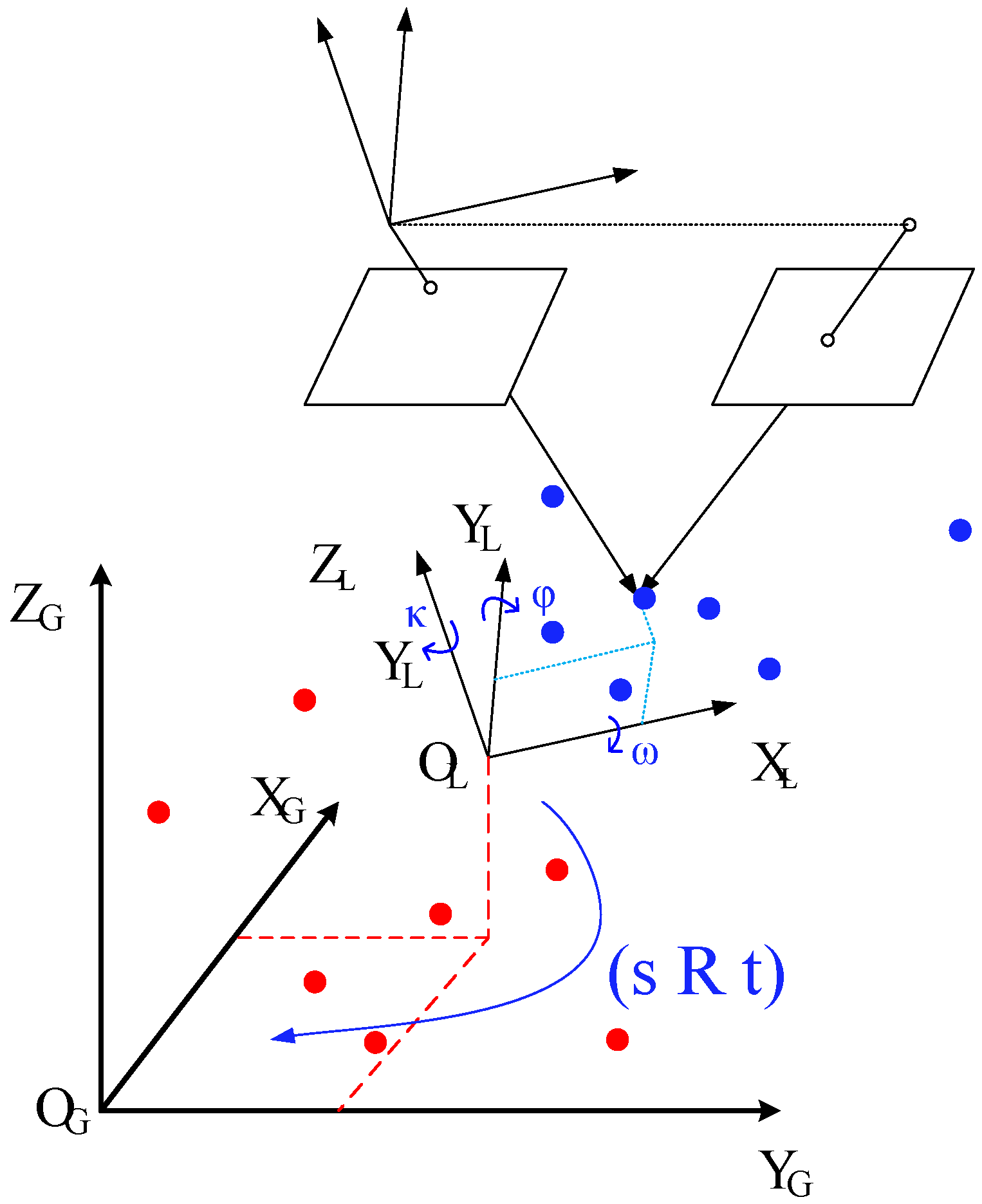
3. Local Similarities Representation

The measurements for the classical non-linear least-squares problem involve all 3D points in the global coordinate reference system. These points are used to optimize the seven similarity transformation parameters for the absolute orientation problem. Here, these 3D points are considered to play the same role in the point transformations, producing similar constraints. However, the distribution of these points can be expected to impact the accuracy with which the absolute orientation problem can be solved.

This section discusses the newly proposed transformation method, which uses the local similarities representation related to the geometric topography of the Ground Control Points (GCPs). A TIN model is used to construct the GCP topography, and various local similarities are computed based on each triangle in the TIN model. The new transformation is then estimated based on these local similarities. Unlike in the classical absolute orientation method, the number of sets of estimated transformation parameters is not one but rather equal to the number of local points, which should be transformed into the global coordinate reference. These sets of estimated transformation parameters are used to directly transform points in the local coordinate reference system into the global coordinate reference system. A weighting function is proposed to combine the various local similarities based on the point distribution.

3.1. Generation of the Triangular Irregular Network Model

TINs are digital data structures that are widely used to represent surfaces in geographic information system (GIS) and photogrammetry studies [18,19]. The first TIN model was proposed in the early 1970s as a simple method for building a surface using a set of irregularly spaced points. TIN models can be broadly applied because of the manner in which they describe and preserve spatial relationships [20,21]. A TIN model is used in the proposed transformation method to divide a region into numerous adjacent triangles using the given GCPs, which are located on the vertices of these triangles in the local coordinate reference system. Seven similarity transformation parameters can then be retrieved using the three pairs of GCPs from each triangle. The similarity transformations thus retrieved from each triangle are called the local similarities, which best represent the relationships between two corresponding triangles in the two coordinate reference systems. The TIN model is constructed from the GCPs such that the Delaunay triangle criterion is satisfied at the local scale, meaning that a circle that passes through the three GCPs of a given triangle will not contain any other points. The minimum interior angles of all triangles are maximized when all such circles passing through three GCPs satisfy the Delaunay criterion.

The triangulation growth algorithm [22] illustrated in Figure 3 is used to generate the TIN model from the GCPs. A simple example of TIN construction using 15 GCPs is explained as follows:

(1) initial Delaunay triangle generation. First, locate a GCP “A” that is close to the geometric center of all GCPs. Then, search for the initial base line AB by finding another point “B” that is closest to “A”. The initial Delaunay triangle is generated by finding a third point “C” that satisfies the Delaunay triangle criterion;

(2) triangular network growth. The three closest points “D”, “E” and “F” that satisfy the Delaunay criterion for each edge of the initial triangle are identified;

(3) TIN model construction. The triangular network is developed by repeating (2) until all of the GCPs have been incorporated as triangle vertices.

3.2. Estimation of the New Transformation Based on Local Similarities

A set of seven similarity parameters can be effectively estimated from three GCPs, as stated in Section 2. Various sets of seven similarity transformation parameters can thus be obtained, each from a different set of three triangle vertices. Such a set of similarity transformation parameters based on three triangle vertices is called a local similarity, and these local similarities are used to estimate the new transformation proposed in this study.

Suppose that n triangles exist for a given point set containing N pairs of GCPs and their corresponding local points. Various sets of local transformation parameters $(s_i,R_i,t_i)$ can be retrieved from each triangle $i(1\le i\le n)$ using the method described in Section 2. Each triangle exerts a different influence when transforming a local coordinate reference Check Point (CP) $P_L$ to the global coordinate CP $P_G$ . Thus, the local coordinate $P_L$ can be transformed to the global coordinate $P_G$, the proposed transformation, which is a function of the local similarities, as follows:

$$P_G^j=f(w_1,s_1,R_1,t_1,...w_i,s_i,R_i,t_i,...,w_n,s_n,R_n,t_n,)P_L=\sum _{i=1}^n{w}_i\left(P_L^j\right)[s_i{R}_i{P}_L^j+t_i]$$

(3)

where $w_i\left(P_L^j\right)$ is the weight of the $i^{th}$ triangle, which is determined by a weighting function that will be discussed in the next section. This function defines the contributions of the various local similarities to the point transformation of $P_L^j$.

The eight GCPs and the CP (A) illustrated in Figure 4 provide a simple example. Eight triangles are constructed based on the TIN model, in which each vertex corresponds to a GCP. The three vertices of each triangle are used to obtain eight local similarities, which can be written as $\{(s_i,R_i,t_i),i=1,2,...,8\}$. Meanwhile, the weights of the eight triangles are denoted by $w_{\Delta 1,2,5},w_{\Delta 2,5,6},w_{\Delta 5,6,8},w_{\Delta 5,7,8},w_{\Delta 4,5,7},w_{\Delta 3,4,7},w_{\Delta 1,3,4}$ and $w_{\Delta 1,4,5}$. Point A, represented by $P_L^A$ in the local coordinate reference system, can be transformed into point $P_G^A$ in the global coordinate reference via:

$$P_G^A=\sum _{i=1}^8{w}_i[s_i{R}_i{P}_L^A+t_i],(w_i\in w_{\Delta 1,2,5},w_{\Delta 2,5,6},w_{\Delta 5,6,8},w_{\Delta 5,7,8},w_{\Delta 4,5,7},w_{\Delta 3,4,7},w_{\Delta 1,3,4},w_{\Delta 1,4,5})$$

(4)

The weighting values should satisfy the following constraint:

$$\sum _{i=1}^n{w}_i\left(P_L^j\right)=1$$

(5)

3.3. Weighting Function for Combining Local Similarities

The weighting function introduced in Equation (3) is used to combine the local similarities calculated from all triangles in the TIN model to estimate the new transformation. This weighting function can be expressed as a function of the point distribution, which can be measured based on the distances between a CP and the three vertices of each triangle in the local coordinate reference system. The weights calculated using the weighting function should be small for triangles far from the CP and large for triangles closer to the CP.

The red dashed lines in Figure 3 represent the distances between a CP and the three vertices of a nearby triangle, whereas the blue dashed lines represent the distances between a CP and the three vertices of a distant triangle. The weight $I_{\Delta 1,2,5}$ of triangle ${\Delta }_{1,2,5}$ with respect to a given CP can be expressed as a power function:

$$I_{\Delta 1,2,5}=\frac{1}{d_{\Delta 1,2,5}^q}=\frac{1}{{(d_{1A}+d_{2A}+d_{5A})}^q}$$

(6)

where $d_{iA}=\sqrt{{(x_i-x_A)}^2+{(y_i-y_A)}^2++{(z_i-z_A)}^2},(1\le i\le 8)$. $d_{1A}$, $d_{2A}$, and $d_{5A}$ represent the distances between the three vertices of the triangle and the CP. The power-law index q is set to 60 for optimal accuracy in this study. The influence of the power-law index on the accuracy is analyzed in detail in Section 4.3.

The constraint in Equation (5) can then be satisfied as follows. For n triangles, the normalized weight of the $i^{th}$ triangle with respect to the $j^{th}$ CP $P_L^i$ is given by

$$w_i\left(P_L^j\right)=\frac{I_i}{I_1+...+I_i+...+I_n}=\frac{\frac{1}{d_i^q}}{\frac{1}{d_1^q}+...+\frac{1}{d_i^q}+\frac{1}{d_n^q}},1\le i\le n$$

(7)

4. Experiments and Discussion

To analyze the performance of the absolute orientation method, two sets of 3D points in two different coordinate reference systems should be provided. For the analysis presented in this paper, the bundle adjustment (BA) method, a type of aerial triangulation, was utilized to generate such 3D points using two-dimensional (2D) image points as input to serve as the measurements for the BA non-linear optimization problem. Note that the proposed method is also valid for other applications besides aerial triangulation. For example, 3D LiDAR points can be transformed between two coordinate systems using the proposed absolute orientation method.

This section reports the use of six simulated data sets and one real data set representing an aerial photogrammetric terrain scenario to assess the accuracies of the classical absolute orientation method and the proposed method. For convenience, 3D points in the global coordinate reference system are called global points, whereas points in the local coordinate reference system are called local points.

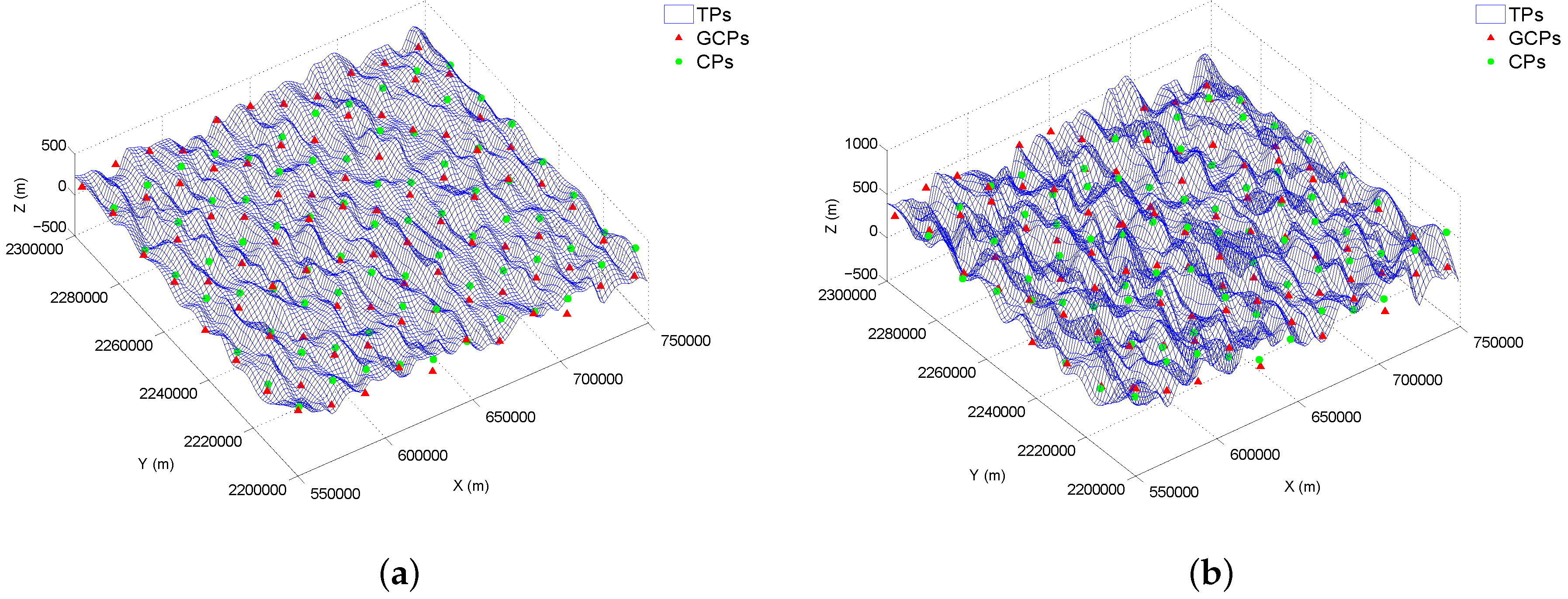
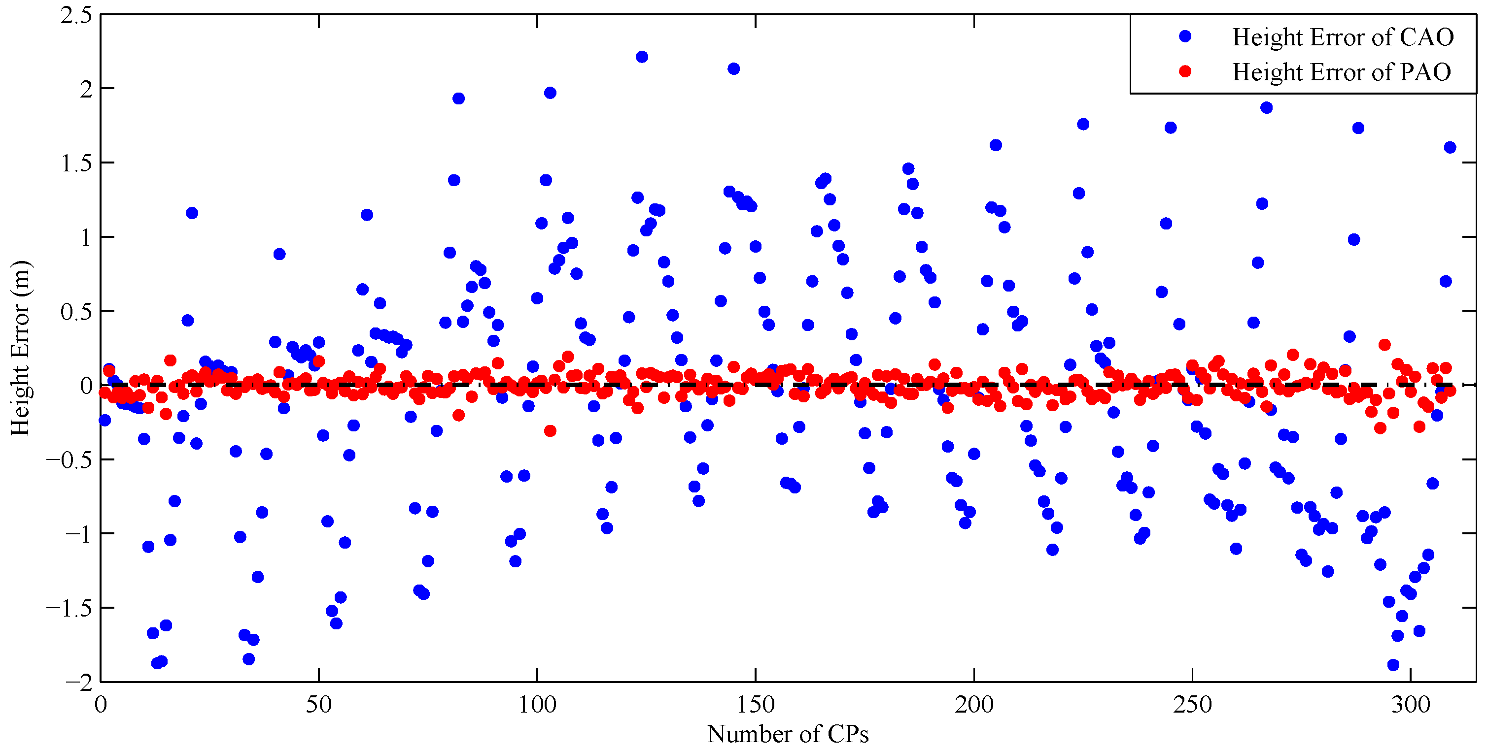
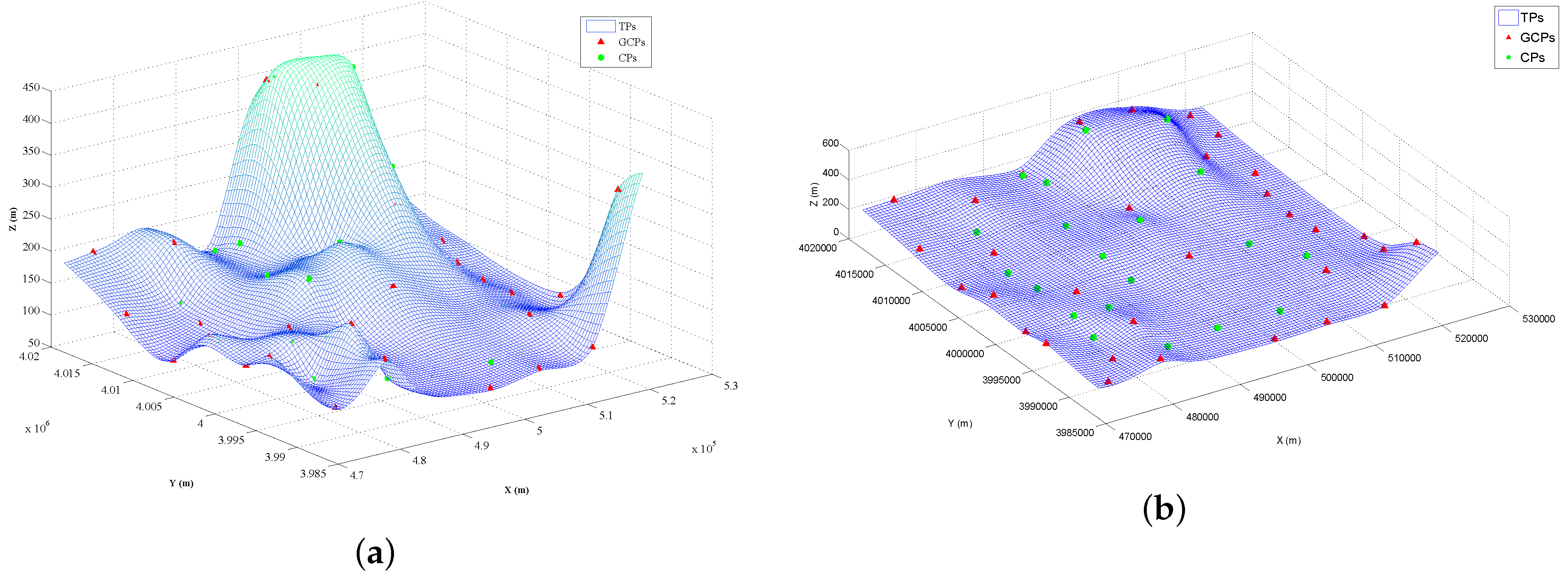
4.1. Simulated Data Sets

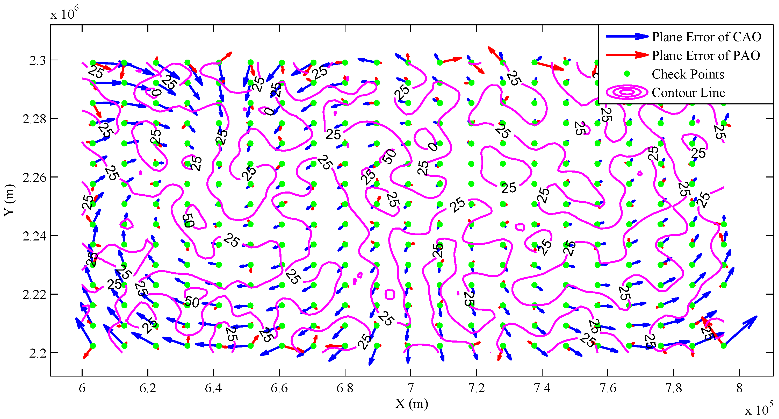
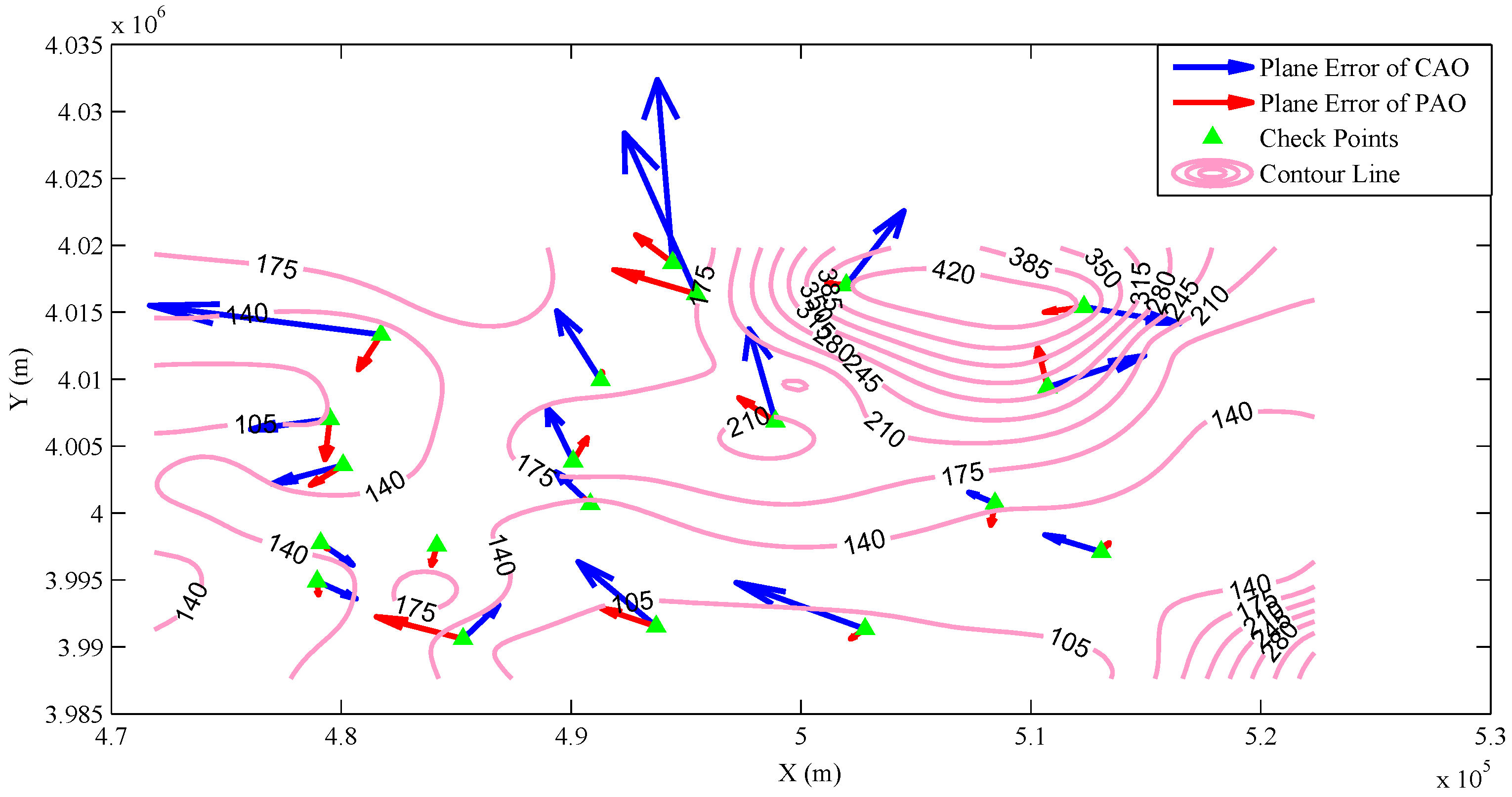
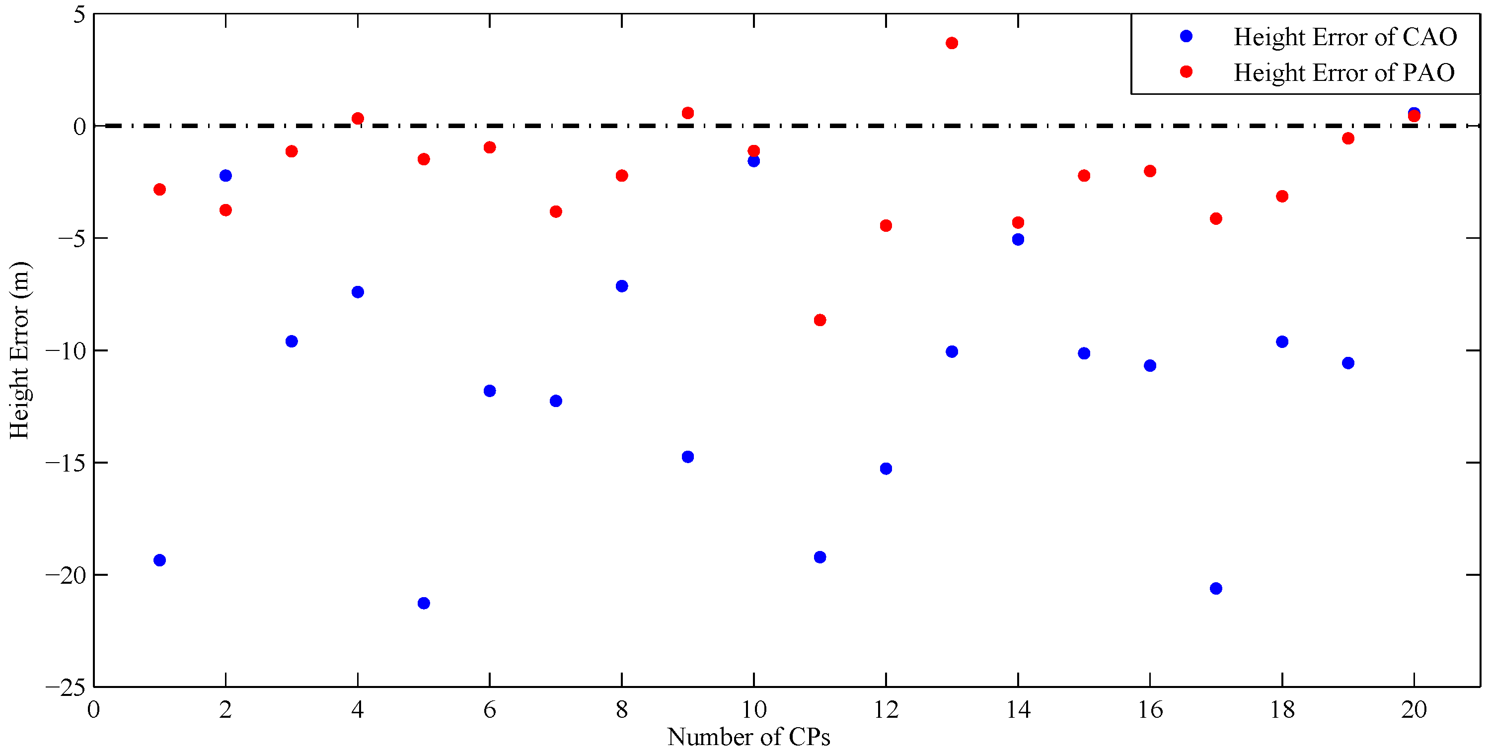
For an aerial triangulation application, the absolute orientation method followed by free-net BA can be used to obtain an initialization for the BA solution with control points (BA–CP). The absolute orientation method can be used to transform 3D tie points and camera poses in the local coordinate reference system to ensure that the initial unknown parameters for BA–CP are located in the global coordinate reference system.

The main workflow for these simulations is explained as follows. When image points of 3D tie points and GCPs are available, these image points can be input into a free-net BA model to simultaneously optimize the exterior orientation (EO) of the camera and the 3D points by minimizing the total difference between the predicted and measured image points. Then, the various 3D points corresponding to the input image points are triangulated. For free-net BA, the origin of the coordinate reference system is often defined as the location of the first camera; thus, these triangulated 3D points should be located in the local coordinate reference system. Now, the local and global coordinates of the GCPs are known, and thus, the transformation parameter estimation is complete. Finally, the global CPs are used to assess the point transformation accuracy of the absolute orientation method.

To obtain 2D image points, it is necessary to generate a synthetic terrain with 3D tie points, GCPs and CPs in the global coordinate reference system. The terrains of the first four data sets in

Table 1. The overall parameters of the four simulation data sets.

Data Set	Height (m)	Scale	Area (km×km)	Image	Strips	GCPs	CPs	Tie Points
Test 1	2500	1:5000	200×100	13772	44	315	309	336362
Test 2	5000	1:10000	200×100	3454	22	88	75	83830
Test 3	7500	1:25000	200×100	1575	15	35	33	37094
Test 4	9500	1:50000	200×100	996	12	24	22	22684
Test 5	5000	1:10000	200×100	3454	22	35	33	37094
Test 6	5000	1:10000	200×100	3454	22	24	22	22684

correspond to village topologies, ranging from approximately 0 m to 50 m in elevation, as illustrated in Figure 5. Additionally, mountain topologies were also simulated in the test data, corresponding to Test 5 and Test 6, as shown in Figure 6. The maximum elevations of the two mountain topologies are approximately 300 m and 500 m, respectively. The numbers of GCPs, CPs and tie points are listed in the eighth, ninth and tenth columns, respectively. In Figure 5 and Figure 6, GCPs and CPs are indicated by red triangles and green circles, respectively. Both the GCPs and CPs are evenly distributed throughout the study area, which encompasses a 200 km × 100 km area. In addition, a Gaussian noise $\sigma =5$ mm were imposed into the planimetric and elevation coordinates of GCPs and CPs in all simulated datasets. The second column refers to the flight height, and the mapping scales are calculated based on a fixed focal length of 0.12 m for the camera used. The areas considered in the six cases are equal, as listed in the fourth column of Table 1.

To generate 3D local points when 3D tie points are available in the global coordinate reference system, 2D image points are first obtained and then input into the BA model. The use of a camera with a maximum image resolution of 7680 × 13,824 pixels that is free of geometric distortion is assumed. The camera is placed at the specified flight height to generate each sequence of aerial images. The forward and side overlaps are as large as 60% and 30%, respectively. The flight trajectories are pre-defined, i.e., the EOs are known. Then, the 3D tie points, GCPs and CPs can be projected onto image films to form 2D image points based on the collinearity equation. These projected image points have zero errors. To make the simulated data more realistic, some noise is added to the projected image points; here, a Gaussian noise of $\sigma =0.3$ pixels is randomly added. These image points with Gaussian noise are input into a free-net BA model to triangulate the local 3D points. Here, ParallaxBA [23] is used as the free-net BA model because of its good performance, including accurate estimation and a rapid convergence rate.

The performance of the proposed method was assessed and validated via comparison with the results of the classical method. The CP accuracies achieved on the six simulated data sets are presented in

Table 2. For simulation data sets, accuracies of CPs are resulted by the classical and proposed methods as well as bundle adjustment with additional GCPs parameters (BA–CP).

Dataset	Method	RMSE x (m)	RMSE y (m)	RMSE Plane (m)	RMSE z (m)
Test 1	CAO	0.324	0.287	0.433	0.866
	PAO	0.015	0.015	0.021	0.077
	BA–CP	0.008	0.010	0.009	0.064
Test 2	CAO	0.298	0.278	0.408	0.608
	PAO	0.037	0.041	0.055	0.165
	BA–CP	0.016	0.023	0.020	0.150
Test 3	CAO	0.329	0.354	0.483	0.640
	PAO	0.055	0.059	0.080	0.297
	BA–CP	0.025	0.036	0.031	0.270
Test 4	CAO	0.141	0.251	0.288	1.649
	PAO	0.050	0.081	0.095	0.439
	BA–CP	0.032	0.058	0.047	0.283
Test 5	CAO	0.141	0.251	0.288	1.649
	PAO	0.050	0.081	0.095	0.439
	BA–CP	0.016	0.022	0.019	0.152
Test 6	CAO	0.141	0.251	0.288	1.649
	PAO	0.050	0.081	0.095	0.439
	BA–CP	0.017	0.023	0.020	0.147

, where CAO and PAO refer to the classical absolute orientation method and the proposed absolute orientation method, respectively. Columns three through six represent the RMSEs in the x-, y- and z-directions. The proposed method yielded improved accuracies for all data sets compared with the classical method. For example, the plane and z RMSE values for Test 1, corresponding to a flight height of 2500 m, were reduced from 0.433 m and 0.866 m to 0.021 m and 0.077 m, respectively, corresponding to increases in the plane and z accuracies by factors of 21 and 11, respectively. This accuracy increase can be attributed to the consideration of the deformation between the two coordinate reference systems, which is not addressed in the classical method. Noise is present in the extracted image points, which introduces error that is propagated into the triangulated points. Thus, reconstructed terrain deformation occurs between the local and global coordinate reference systems. The classical transformation between the two coordinate systems uses a rigid-body transformation and assumes that a single similarity transformation with seven degrees of freedom can sufficiently represent the transformation of deformed objects. However, this assumption cannot simultaneously satisfy the transformation requirements for two deformed objects. Therefore, the proposed method utilizes a representation based on local similarities to express the relationship between the two coordinate systems instead of only a single similarity transformation, thereby decreasing the deformation induced by the noise in the image points.

In addition, another method, BA–CP, was tested for comparison with the absolute orientation methods, as shown in Table 2. It is evident that BA–CP showed the best accuracy among the three methods, although that of the proposed method is only slightly poorer. Clearly, for aerial triangulation, the BA–CP method cannot be entirely replaced by the absolute orientation method. However, the primary purpose of this paper is to improve the accuracy of the point transformation that can be achieved using the classical absolute orientation method.

Finally, the CP errors in the plane and z-directions are presented to illustrate the error distribution. Only the plane and z errors from Test 1 are shown in Figure 7 and Figure 8. The green triangles and purple curves in Figure 7 represent the CPs and contour lines, respectively. The blue and red arrows represent the error directions and magnitudes. The horizontal and vertical axes are scaled by factors of 10,000 and 100,000, respectively, for clarity. The z-direction error distributions of each CP were assessed for both methods, and the results are plotted in Figure 8. The blue and red points represent the residual errors of the classical and proposed methods, respectively. Figure 7 and Figure 8 demonstrate that the plane and z errors of the proposed method are generally smaller than those of the classical method.

The time consumed by the classical and proposed absolute orientation methods are presented in

Table 3. Time consumed by the classical and proposed method using the simulated data sets.

Methods	Test 1	Test 2	Test 3	Test 4	Test 5	Test 6
CAO	0.013	0.011	0.008	0.005	0.009	0.009
PAO	3.930	0.272	0.066	0.022	0.265	0.272

. The efficiency of the proposed method is found to be slightly poorer than that of the classical one. The primary reason for this finding is that only one set of similarity transformation parameters must be calculated in the classical method, whereas it is necessary to compute numerous sets of transformation parameters using Equation (3) in the proposed method.

4.2. Real Data Set

The local and global 3D points of the real data set used to assess the performance of the absolute orientation methods were generated in a manner similar to that described in Section 4.1. However, unlike in the case of the simulated data sets, the 2D image points could be extracted using point feature extraction technology.

The real data set considered here includes 737 Digital Mapping Camera System (DMC) images captured at a height of approximately 3500 m and encompassing an area of 53 km × 35 km. The mapping scale for this data set is 1:30,000. The images are distributed among 12 tracks, of which the forward and side overlaps are as large as 60% and 30%, respectively. Fifty-two 3D points are available in the global Beijing-54 coordinate reference system [24]. In addition, image points for these 3D points are also available. Thirty-two evenly distributed 3D points were chosen as GCPs, and the remaining points were treated as CPs. The 3D coordinates of GCPs and CPs were supplied by a surveying and mapping corporation. Their planimetric accuracies were better than $\pm 10$ mm, while elevation accuracies measured by traditional leveling survey were up to $\pm 5$ mm. The GCP and CP distributions are shown in Figure 9.

A feature extraction and matching algorithm was used to extract 2D image point associations to link adjacent images and provide constraints for the non-linear least-squares optimization problem addressed by the absolute orientation method. A Scale Invariant Feature Transformation ($L^2$-SIFT) algorithm [25] was used because it can effectively process large-scale aerial photogrammetry data. The local 3D points could be triangulated in the local coordinate reference system based on the extracted image points and 3D image points used to solve the BA least-squares problem. The coordinate origin is commonly defined based on the first camera. These triangulated 3D local points corresponded to the input image point associations. Thus, the local points corresponding to the GCPs and CPs could also be obtained.

Based on the criteria of the TIN generation illustrated in Figure 3, we divided all GCPs into the subsets of numerous irregular TIN triangles. For each irregular TIN triangle, the local similarity could be optimized using three pair of the vertices of the triangle. Thus, the number of estimated local similarities were equal to that of the triangles. To achieve the transformation for each CP, the global similarity of the CP can be estimated by combining all local similarities based on the previously described power function. The RMSEs in all four directions were evaluated after the transformation of the local points into the Beijing-54 coordinate reference system using the proposed method, as shown in

Table 4. RMSEs achieved for the real data set using the classical and proposed methods as well as bundle adjustment with additional GCPs parameters (BA–CP).

Method	RMSE x (m)	RMSE y (m)	RMSE Plane (m)	RMSE z (m)
CAO	0.650	0.973	1.170	12.485
PAO	0.302	0.325	0.444	3.250
BA–CP	0.251	0.392	0.329	1.278

. The second row of Table 4 presents the results for the classical method. The RMSEs of the proposed method are presented in the third row.

The x-, y- and z-direction RMSEs of the proposed method were approximately two, three and three times smaller, respectively, than those of the classical method. The plane- and z-direction error distributions for 22 CPs are shown in Figure 10 and Figure 11, where the errors of the proposed method are again less than those of the classical method. In Figure 10, the x- and y-axes are scaled by a factor of 5000. The amounts of time consumed by the classical and proposed absolute orientation methods were 0.002 and 0.026 s, respectively.

Similar to the experimental summary presented in Table 2, the results of the two absolute orientation methods are compared with those of the BA–CP method in Table 4. It is clear that the accuracy of the proposed method is very close to that of BA–CP.

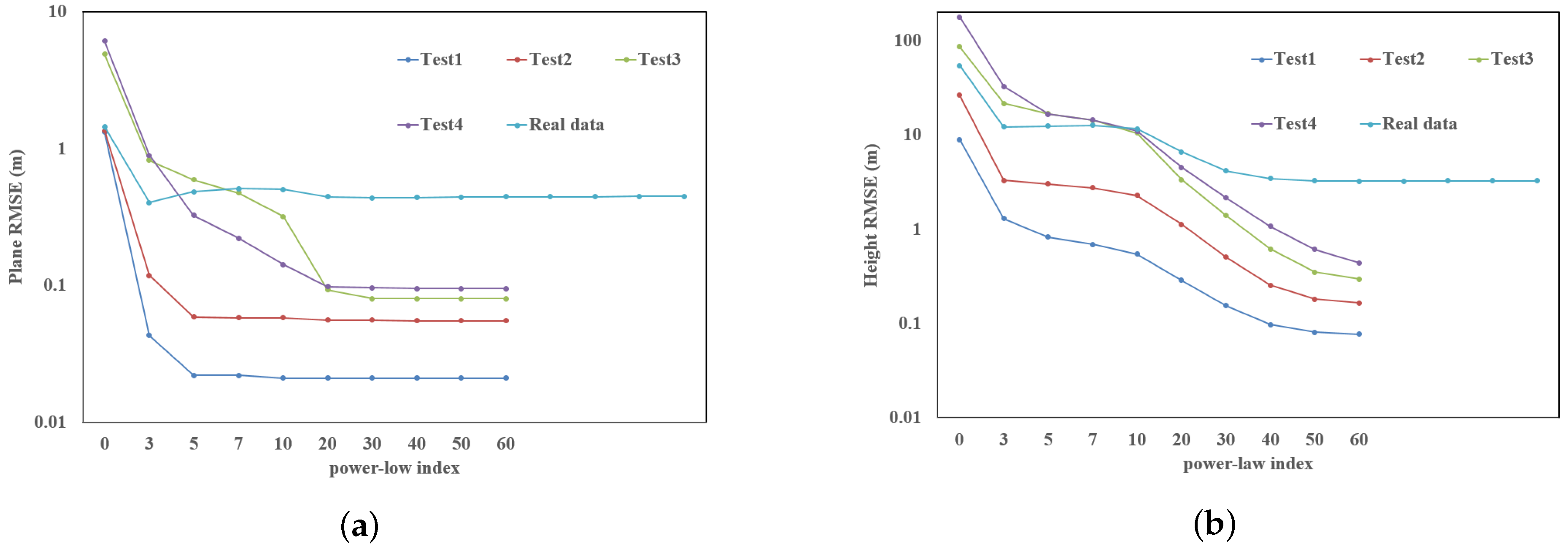
4.3. Analysis of the Influence of the Power-Law Index on the Accuracy of the Proposed Method

The power-law index in Equation (6) plays a very important role in the weighting function, which assigns different weights to different triangles depending on the distance between the CP and the triangle. In this section, the influence of this power-law index on the accuracy of the proposed method is analyzed based on the results of the experiments. Here, the first four data sets in Table 1 and the real data set in Table 2 are used.

The plane and height RMSEs achieved using the proposed method when the power law-index is set to 0, 3, 5, 7, 10, 20, 30, 40, 50, 60, 70, 80, 90 and 100 are listed in

Table 5. RMSEs (m) obtained using various power-law indices.

	Test 1		Test 2		Test 3		Test 4		Real Data
q	Plane	$z$	Plane	$z$	Plane	$z$	Plane	$z$	Plane	$z$
0	1.321	8.973	1.359	26.474	4.919	86.501	6.135	178.301	1.452	54.439
3	0.043	1.300	0.118	3.298	0.821	21.637	0.892	32.706	0.404	12.213
5	0.022	0.825	0.059	3.035	0.592	16.752	0.325	16.675	0.485	12.487
7	0.022	0.690	0.058	2.746	0.476	14.344	0.221	14.485	0.511	12.682
10	0.021	0.547	0.058	2.284	0.319	10.489	0.142	11.029	0.503	11.591
20	0.021	0.288	0.056	1.124	0.093	3.359	0.098	4.557	0.445	6.636
30	0.021	0.155	0.056	0.507	0.080	1.396	0.096	2.151	0.435	4.175
40	0.021	0.098	0.055	0.256	0.080	0.616	0.095	1.073	0.439	3.451
50	0.021	0.081	0.055	0.182	0.080	0.352	0.095	0.611	0.442	3.282
60	0.021	0.077	0.055	0.165	0.080	0.297	0.095	0.439	0.444	3.250
70	N/A	N/A	N/A	N/A	N/A	N/A	N/A	N/A	0.445	3.252
80	N/A	N/A	N/A	N/A	N/A	N/A	N/A	N/A	0.446	3.261
90	N/A	N/A	N/A	N/A	N/A	N/A	N/A	N/A	0.447	3.270
100	N/A	N/A	N/A	N/A	N/A	N/A	N/A	N/A	0.447	3.278

. In addition, the plane and height RMSEs are plotted as a function of the power-law index in Figure 12. The RMSEs are very large when the index is set to zero and the weights calculated using Equation (6) are always one. This means that the weighting is unaffected by the distance between the CP and the triangle. This situation disobeys the underlying assumption of the proposed method, namely, that a closer triangle (at a smaller distance) should have a greater contribution to the transformation of a CP. As the power-law index increases, the accuracies continuously improve, primarily because larger and smaller contributions are assigned to closer and farther triangles, respectively, when this parameter is large. However, once the index becomes very large (e.g., 70 for the simulated data sets), the transformation fails. The primary reason for this failure is that the denominator in Equation (6) tends toward infinity, causing the weight of each triangle to become zero when the power-law index is large, and consequently, the normalization of the weights in Equation (7) fails because the denominator also becomes equal to zero.

In summary, when the power-law index is set to 60, the best accuracy can be obtained for data presented in Table 1. Thus, the power-law index 60 is used for the experiments in Section 4.1 and Section 4.2 of this study.

5. Conclusions

A new absolute orientation method is proposed to accurately transform points between local and global (geodetic) coordinate reference systems. The transformation uses multiple local similarities instead of a single similarity transformation. The GCPs are divided into numerous subsets based on the generation of a TIN. The local similarities can be individually estimated by minimizing the differences between the fitted points and the three vertices of a triangle. The new transformation is obtained by combining the various local similarities. The results suggest that the x-, y- and z-direction RMSEs can be improved by factors as large as 22, 20 and 21, respectively, based on a simulated data set acquired at a height of 2500 m. Additionally, for a real data set, these RMSEs can be reduced by factors of approximately two, three and three, respectively, compared with the classical method. In addition, the accuracies of both the classical and proposed absolute orientation methods are compared with that of another method, BA–CP. Clearly, the BA–CP method cannot be replaced by absolute orientation methods as the method that offers the best accuracy for aerial triangulation. However, for other applications in which image points are not available, the BA–CP method will fail, and the proposed method can provide a feasible solution for point transformation.

At present, the automatic determination of the optimal power-law index is a complex task. Future work will primarily focus on how to robustly determine this parameter.

References

1. Biljecki, F.; Stoter, J.; Ledoux, H.; Zlatanova, S.; Çöltekin, A. Applications of 3D city models: State of the art review. ISPRS Int. J. Geo-Inf. 2015, 4, 2842–2889. [Google Scholar]
2. Nebiker, S.; Cavegn, S.; Loesch, B. Cloud-Based geospatial 3D image spaces—A powerful urban model for the smart city. ISPRS Int. J. Geo-Inf. 2015, 4, 2267–2291. [Google Scholar] [CrossRef]
3. Ohori, K.A.; Ledoux, H.; Biljecki, F.; Stoter, J. Modeling a 3D city model and its levels of detail as a true 4D model. ISPRS Int. J. Geo-Inf. 2015, 4, 1055–1075. [Google Scholar] [CrossRef]
4. Hildebrandt, D. A software reference architecture for service-oriented 3D geovisualization systems. ISPRS Int. J. Geo-Inf. 2014, 3, 1445–1490. [Google Scholar] [CrossRef]
5. Virtanen, J.-P.; Hyyppä, H.; Kämäräinen, A.; Hollström, T.; Vastaranta, M.; Hyyppä, J. Intelligent open data 3D maps in a collaborative virtual world. ISPRS Int. J. Geo-Inf. 2015, 4, 837–857. [Google Scholar] [CrossRef]
6. Gregory, A.; Lipczynski, R. T. The three dimensional reconstruction of human facial images. In Proceedings of the 15th Annual International Conference on Engineering in Medicine and Biology Society, San Diego, CA, USA, 28–31 October 1993.
7. Liu, Z.; Qin, H.; Bu, S.; Yan, M.; Huang, J.; Tang, X.; Han, J. 3D real human reconstruction via multiple low-cost depth cameras. Signal Process. 2015, 112, 162–179. [Google Scholar] [CrossRef]
8. Van den Heuvel, F.A. 3D reconstruction from a single image using geometric constraints. ISPRS J. Photogramm. Remote Sens. 1998, 53, 354–368. [Google Scholar] [CrossRef]
9. Yang, L.; Sheng, Y.; Wang, B. 3D reconstruction of building facade with fused data of terrestrial LiDAR data and optical image. Optik - Int. J. Light Electron Opt. 2016, 127, 2165–2168. [Google Scholar] [CrossRef]
10. Virtanen, J.-P.; Hyyppä, H.; Kurkela, M.; Vaaja, M.; Alho, P.; Hyyppä, J. Rapid prototyping —A tool for presenting 3-dimensional digital models produced by terrestrial laser scanning. ISPRS Int. J. Geo-Inf. 2014, 3, 871–890. [Google Scholar] [CrossRef]
11. Zhang, F.; Huang, X.; Fang, W.; Zhang, Z.; Li, D.; Zhu, Y. Texture reconstruction of 3D sculpture using non-rigid transformation. J. Cult. Herit. 2015, 16, 648–655. [Google Scholar] [CrossRef]
12. Mikhail, E.M.; Bethel, J.S.; McGlone, J.C. Introduction to Modern Photogrammetry; John Wiley and Sons Inc.: Hoboken, NJ, USA, 2001. [Google Scholar]
13. Blostein, S.; Huang, T. Estimating 3-D motion from range data. In Proceedings of the 1st Conference on Artificial Intelligence Applications, Denver, CO, USA, 1 February 1984.
14. Horn, B.K.P.; Hilden, H.M.; Negahdaripour, S. Closed-form solution of absolute orientation using orthonormal matrices. J. Opt. Soc. Am. A 1988, 5, 1127–1135. [Google Scholar] [CrossRef]
15. Arun, K.S.; Huang, T.S.; Blostein, S.D. Least-squares fitting of two 3-D point sets. IEEE Trans. Pattern Anal. Machine Intell. 1987, 5, 698–700. [Google Scholar] [CrossRef]
16. Schenk, T. Introduction to Photogrammetry; The Ohio State University: Columbus, OH, USA, 2005. [Google Scholar]
17. Umeyama, S. Least-squares estimation of transformation parameters between two point patterns. IEEE Trans. Pattern Anal. Machine Intell. 1991, 4, 376–380. [Google Scholar] [CrossRef]
18. Ali, T.; Mehrabian, A. A novel computational paradigm for creating a Triangular Irregular Network (TIN) from LiDAR data. Nonlinear Anal. 2009, 71, e624–e629. [Google Scholar] [CrossRef]
19. Chini, M.; Atzori, S.; Trasatti, E.; Bignami, C.; Kyriakopoulos, C.; Tolomei, C.; Stramondo, S. The 12 May 2008, (Mw 7.9) Sichuan earthquake (China): Multiframe ALOS-PALSAR DInSAR analysis of coseismic deformation. IEEE Geosci. Remote Sens. Lett. 2010, 7, 266–270. [Google Scholar] [CrossRef]
20. Nguyen, V.T. In Building TIN (triangular irregular network) problem in Topology model. In Proceedings of the 2010 International Conference on Machine Learning and Cybernetics (ICMLC), Qingdao, China, 11–14 July 2010; pp. 14–21.
21. Silva, C.T.; Mitchell, J.S.B.; Kaufman, A.E. Automatic generation of triangular irregular networks using greedy cuts. In Proceedings of the 6th Conference on Visualization ’95, Washington, DC, USA, 29 October 1995; pp. 201–208.
22. Lu, T. Research on the Total Least Squares and Its Applications in Surveying Data Processing. Ph.D. Thesis, Wuhan University, Wuhan, China, 2010. [Google Scholar]
23. Zhao, L.; Huang, S.; Sun, Y.; Yan, L.; Dissanayake, G. ParallaxBA: Bundle adjustment using parallax angle feature parametrization. Int. J. Robot. Res. 2015, 34, 493–516. [Google Scholar] [CrossRef]
24. Wang, W.; Wu, J.; Fang, L.; Zeng, K.; Chang, X. Design and implementation of spatial database and geo-processing models for a road geo-hazard information management and risk assessment system. Environ. Earth Sci. 2015, 73, 1103–1117. [Google Scholar] [CrossRef]
25. Sun, Y.; Zhao, L.; Huang, S.; Yan, L.; Dissanayake, G. L2-SIFT: SIFT feature extraction and matching for large images in large-scale aerial photogrammetry. ISPRS J. Photogramm. Remote Sens. 2014, 91, 1–16. [Google Scholar] [CrossRef]
Figure 1. Three rotation angles and the corresponding axes.
Ijgi 05 00135 g001
Figure 2. Three-dimensional (3D) points transformed from a local coordinate reference ( O L - X L Y L Z L ) to a global reference ( O G - X G Y G Z G ) using the classic absolute orientation method.
Ijgi 05 00135 g002
Figure 3. The TIN model generation procedure using GCPs for the absolute orientation problem.
Ijgi 05 00135 g003
Figure 4. A simple example of the proposed transformation based on local similarities.
Ijgi 05 00135 g004
Figure 5. The GCP and CP distributions for the first to fourth simulated data sets. (a) Test 1; (b) Test 2; (c) Test 3; (d) Test 4. The red triangles and green circles represent GCPs and CPs, respectively. Additionally, Tie Points (TPs) are drawn with blue quadrangles.
Ijgi 05 00135 g005
Figure 6. The GCP and CP distributions for the fifth and sixth simulated data sets. (a) Test 5; (b) Test 6. The red triangles and green circles represent GCPs and CPs, respectively. Additionally, TPs are drawn with blue quadrangles.
Ijgi 05 00135 g006
Figure 7. The 2D plane error distributions for each CP from the simulated data set for Test 1 assessed for the classical absolute orientation method (CAO) and the proposed absolute orientation method (PAO).
Ijgi 05 00135 g007
Figure 8. The z-direction errors for each CP from the simulated Test 1 data set assessed for the classical absolute orientation method (CAO) and the proposed absolute orientation method (PAO).
Ijgi 05 00135 g008
Figure 9. The GCP and CP distributions for the real data set. (a) Side View. (b) Top View. The red triangles and green circles represent GCPs and CPs, respectively. Additionally, TPs are drawn with blue quadrangles.
Ijgi 05 00135 g009
Figure 10. The 2D plane error distributions of 22 CPs in the real data set assessed for the CAO method and the PAO method.
Ijgi 05 00135 g010
Figure 11. The height error distributions of each CP in the real data set assessed for the classical absolute orientation method (CAO) and the proposed absolute orientation method (PAO).
Ijgi 05 00135 g011
Figure 12. The plane and height RMSEs as functions of the power-law index in Equation (6). (a) Plane RMSEs; (b) Z RMSEs.
Ijgi 05 00135 g012