A New Simplification Approach Based on the Oblique-Dividing-Curve Method for Contour Lines

Abstract

As one of the key operators of automated map generalization, algorithms for the line simplification have been widely researched in the past decades. Although many of the currently available algorithms have revealed satisfactory simplification performances with certain data types and selected test areas, it still remains a challenging task to solve the problems of (a) how to properly divide a cartographic line when it is too long to be dealt with directly; and (b) how to make adaptable parameterizations for various geo-data in different areas. In order to solve these two problems, a new line-simplification approach based on the Oblique-Dividing-Curve (ODC) method has been proposed in this paper. In this proposed model, one cartographic line is divided into a series of monotonic curves by the ODC method. Then, the curves are categorized into different groups according to their shapes, sizes and other geometric characteristics. The curves in different groups will trigger different strategies as well as the associated criteria for line simplification. Whenever a curve is simplified, the whole simplified cartographic line will be re-divided and the simplification process restarts again, i.e., the proposed simplification approach is iteratively operated until the final simplification result is achieved. Experiment evidence demonstrates that the proposed approach is able to handle the holistic bend-trend of the whole cartographic line during the simplification process and thereby provides considerably improved simplification performance with respect to maintaining the essential shape/salient characteristics and keeping the topological consistency. Moreover, the produced simplification results are not sensitive to the parameterizations of the proposed approach.

1. Introduction

Following the developments of information techniques, it became necessary to automate tasks that were previously manual such as map generalization between various representations used for digital cartography and/or geographical information science (GIS).

As one of the key operators of map generalization, line generalization is considered one of the most complex processes in cartographic data production [1]. It is a data reduction process used to (a) improve the display quality; (b) allow data analysis with different degrees of detail; and (c) reduce data storage requirements when for example the scale is decreased. Given a cartographic curve, a line simplification algorithm aims to generate simplified cartographic lines with lower granularity without changing the amount of geographic features and destroying their essential shapes or salient characters [1,2,3,4,5].

Due to the fact that most geographic features use lines as the basic entity for their representation on typical cartographic maps, the topic of line simplification has been widely and deeply investigated in the past decades [6,7,8,9]. Previous research has yielded a number of algorithms to reduce the granularity of lines while preserving the major geometric characteristics [10,11,12].

The classic Douglas-Peucker (DP) algorithm, known as one of the most popular line simplification methods, can select important vertices based on a predefined tolerance distance [13]. After removing the unimportant vertices, the curve simplified by DP algorithm could be displaced by a distance up to the predefined tolerance and therefore may lose proper topological relationships to itself (self-intersection) and/or other geographic features lying very near. Extending the DP algorithm, Saalfeld [14] has provided an efficient rule for selecting some specific vertices to be added to the simplified feature, which helps to avoid potential topological conflicts of the feature with itself and other nearby features. Instead of relying on the tolerance distance employed by DP algorithm, Visvalingam and Whyatt [15] suggest to remove the vertices forming the triangles with smallest “effective area” for the task of line simplification. In some situations, however, the Visvalingam and Whyatt (VW) algorithm fails to produce reasonable simplified results because the shape of the measured triangle is not taken into consideration. For instance, a very flat triangle and a very tall triangle of the same area are treated as having the same cartographic significance. To overcome this deficiency, the “weighted effective area” has been implemented to improve the performance of the original VW algorithm in Zhou and Jones [16]. Different from the DP and VW algorithm, Li and Openshaw [17] attempt to realize the line simplification by simulating the natural process by which people observe the objects. This algorithm is based on the so-called natural principle and uses a ratio of input and target resolution to define the “smallest visible object”, which can be employed as a significant criterion to detect and retain the overall shape of a line.

Moreover, Nabil Mustafa et al. [18] presented a so-called Voronoi diagram method, which first divides a complex cartographic curve into a series of safe sets and then simplifies each safe set by using the algorithms such as DP and VW. In this way, it avoided intersections among the lines input. However, Yang et al. [19] argued that such a Voronoi-diagram-based method cannot guarantee the computational precisions and may result in self-intersections. Nöllenburg et al. [11] studied polylines morphing at different scales, which can help to realize continuous generalization for linear geographical features like roads and rivers. Park and Yu [20] proposed a hybrid line simplification method, which has been proved to result in better performance than the single simplification algorithms in terms of the vector displacement. Stanislawski et al. [21] discussed various metric assessments such as segment length, sinuosity, areal displacement, vector displacement and Hausdorff distance for automated line simplification in humid landscapes, which may guide more appropriate parameter-settings over a range of reduced map scales and geographic conditions. Besides, Raposo [22] developed a scale-specific automated line simplification algorithm by vertex clustering on a hexagonal tessellation, which bears similarities to the Li-Openshaw algorithm, with three key differences in terms of sampling geometry, mathematical relation to target scale and line weight, and method of quantization of vertices from multiple line passes within a tessera. Mostly due to the superior radial symmetry and isotropy of the honeycomb sampling geometry, this algorithm offers significantly greater positional fidelity.

In order to achieve the transition from simplification to generalization of natural occurring lines, the approach proposed by Nakos et al. [10] does not only perform the line simplification alone, but also together with the operations of data smoothing, exaggeration, typification, enhancement or any combination of them. Their research constituted great progress towards the full-life-circle data generalization with high automation. Besides contributions on line simplification algorithms, Mustière et al. [23] set up the strategies on how to evaluate the legibility of symbolized lines so as to detect the non-legible part of a line network, which is crucial to the evaluation of data quality after line simplification.

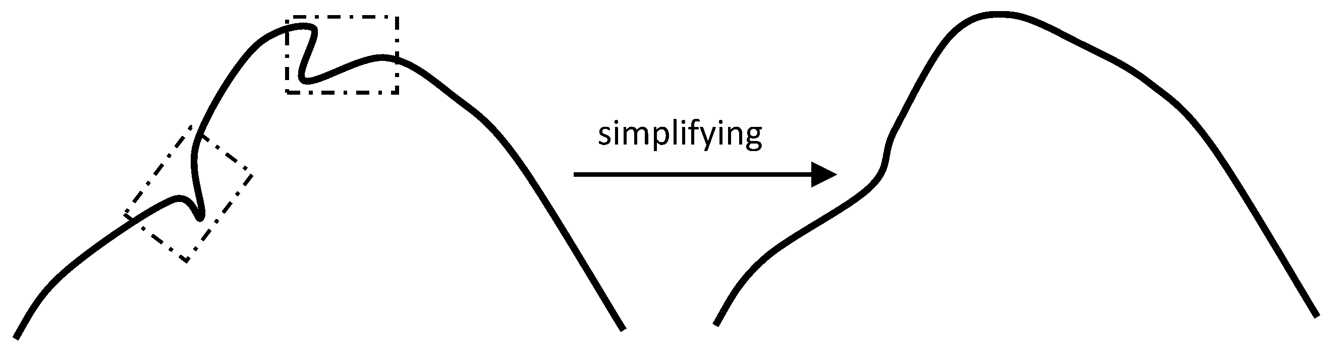
The reported algorithms in the literature so far have doubtlessly paved the way to the development of comprehensive approaches for automatic line simplification. However, unsatisfactory simplified results still exist especially in cases when (a) the cartographic lines to be simplified are too long and too tortuous to be dealt with as a whole; (b) the geometric and/or topologic characteristics of the cartographic lines are so different to each other that it is hard to use a unified parameterization to deal with all of them; and (c) after data simplification, one U-shaped sinuosity tends to be changed to be V-shaped by many currently available algorithms, and vice versa. These problems become more serious when contour lines are processed. This is because the contour lines have continuous natural bending and thus have a more complex structure with much higher bending degree comparing to some other types of line features, such as roads, rivers, power lines, etc.), which can bring more difficulties to line simplifications. Thereby, this article proposes a new data simplification approach for contour lines, which is based on a so-called ODC (Oblique Dividing Curve) method and operates iteratively.

The remainder of this article is organized into 4 parts: (i) Section 2 illustrates the new concept and principles of the so-called OCD method and points out its advantages for the task of line simplification; (ii) in Section 3, the strategy of the iterative line-simplification approach based on OCD method is described in details; (iii) Section 4 reports the experiments applying the proposed approach on a number of real-world data and evaluates the proposed approach in comparison to some other algorithms; and (iv) Section 5 discusses the overall performance and potential improvements of the proposed approach. To avoid tedious descriptions, the terminologies of “polyline and cartographic line”, “sinuosity and bend”, “division and segmentation” are utilized interchangeably.

2. The Oblique-Dividing-Curve (ODC) Method

In case one cartographic line (e.g., contour line) is very long and/or involves many sinuosity, the line needs to be divided into a series of shorter curves (parts) according to certain geometric and topologic characteristics and then each curve should be treated differently in the process of line simplification.

Hoffman and Richards [24] pointed out that the cartographic lines can be cut at minima of curvature. However, the positions of the minima of curvature are not invariant under a change in the direction of traversal, which indicates that the divided curves as specified in its representation can be very different when the orientation is reversed (see Figure 1). Thus, the simplification operation can only consider the bending characters either at “peaks” or “bottoms”, which may lead to quite different simplified results even if the same algorithm has been implemented.

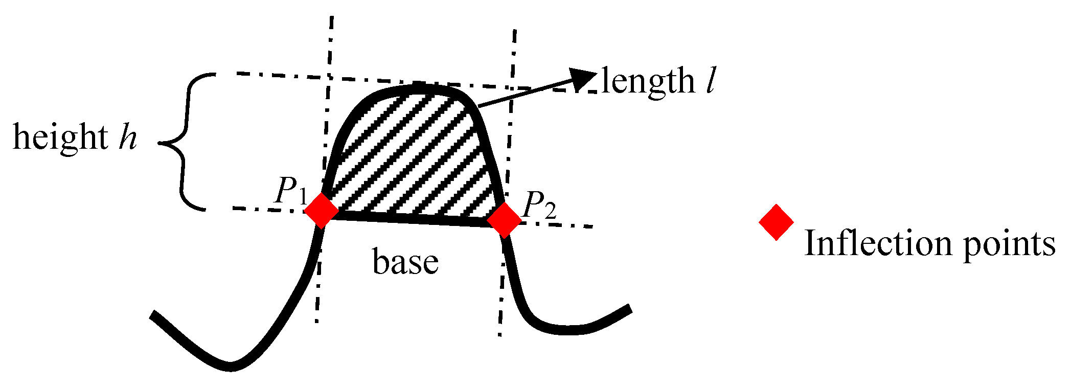
Such an undesirable condition has been refined by Plazanet et al. [25], in which the inflection points are selected as potential locations for line segmentation. After the division, a set of measurements, including the curve height h, the curve length l, the Euclidean distance base between the inflection points, etc., are utilized for the sinuosity classification (see Figure 2). For a given curve, the mean values or median values are computed for all these measurements and then fed into a classical hierarchical clustering process—the sinuosity in different clusters will trigger different simplification strategies, depending on the characteristics. In this way, the performance of line simplification has been dramatically enhanced.

Mitropoulos and Nakos [26] developed a model following the framework of “segmentation, classification and generalization”, where the cartographic lines are divided based on the ɛ-convexity technique introduced by Perkal [27], where a disc with the diameter ε rolls on a cartographic line and thus generate the segmentation points to divide the polyline into ε-convex and ε-non-convex parts. In this work, the parameter corresponds to the size of diameter ε and it is equal to the sum of the visual separation limit, the width of line symbol and a tolerance value expressed at the target scale, which is independent of any individual intervention at a given generalization task.

As depicted above, most of the dividing methods in existing literature are statically operated. That is, after the segmentation, the dividing points remain unchanged during the whole process of the data simplification. Thus, discrete distortions around the dividing points may result and the whole cartographic line could become unsmooth at the dividing points after the data simplification.

To fill this gap in existing studies, the authors have developed a brand-new dividing method in this article, termed as the Oblique-Dividing-Curve (ODC) method (see detailed illustrations from Section 2.1, Section 2.2 and Section 2.3). Different from existing dividing methods that are mostly static, the ODC method is a dynamic dividing method that implements an iteratively-processed strategy for line segmentation. That is, whenever a curve is simplified, the whole cartographic line will be re-divided and the line simplification process restarts again (ref. Section 3.3).

2.1. Basic Principle of the ODC Method

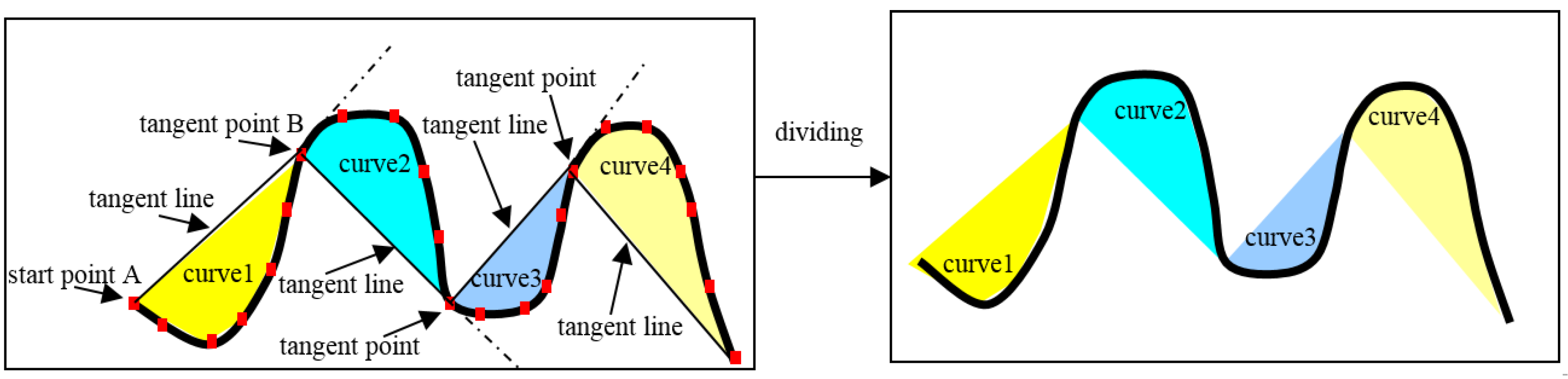
The principle of the ODC method can be depicted by Figure 3. First, point A on the cartographic line is randomly selected as the starting point. Starting from point A, the tangent can be drawn to its nearest bend. Thus, the segment between point A and the point of tangency (viz. point B) forms a new curve (viz. curve 1). In other words, the initial cartographic line is divided into two parts—curve 1 and the rest. Then, point B is treated as the new “starting point” and the rest of the cartographic line can be divided analogously (see curves 2~4 in Figure 3). After the division, the generated curves (see curve 1~4 in Figure 3) involve not only peaks but also valleys.

Note that the terms of “tangent” and “point of tangency” mentioned in this article do not comply with the strict mathematical definition. Instead, they are deployed to illustrate the general concepts/ideas for the line division. Specific computing principle to identify such “tangent” and “point of tangency” can be found in steps 3~4 in Section 2.2.

One of the key factors in the line-simplification process is to keep the general geometric characteristics of the bending parts of a cartographic line. As illustrated by Figure 4, no matter which direction the ODC method starts from, the geometric characteristics of both ‘bottoms’ and ‘peaks’ can be commendably retained, which indicates the ODC method can consider more comprehensive geometric characteristics comparing to some traditional methods of ‘line segmentation’.

2.2. Schematic Process of the ODC Method

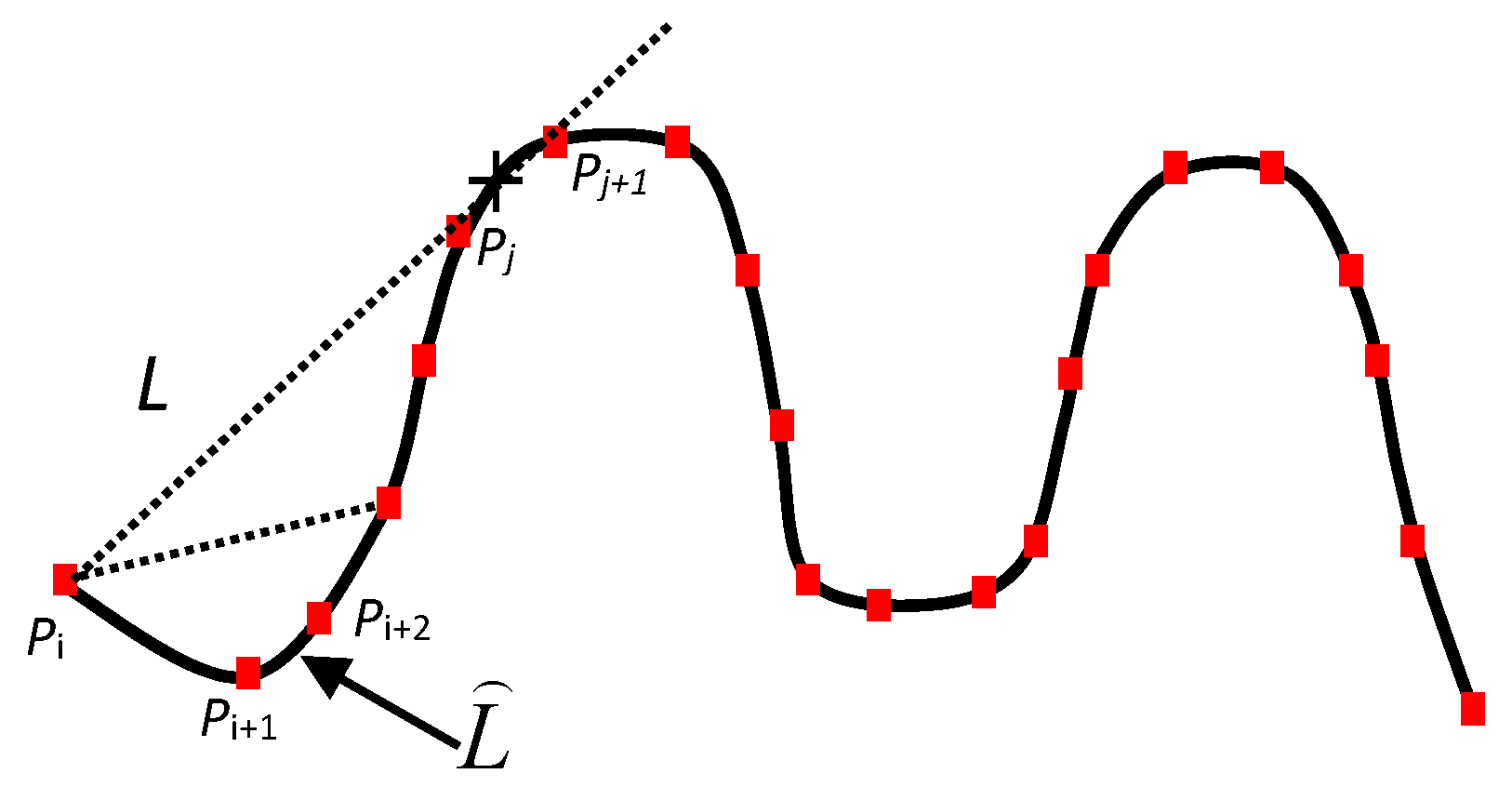
Let $\widehat{L}=\{P_1,P_2,\dots ,P_i,\dots P_n,i\in N\}$ represent the cartographic line to be simplified, L_ij represent the straight line connected by the points P_i and P_j, and ${\widehat{L}}_{ij}$ represent the curve formed by the points P_i, P_{i + 1}, P_{i + 2}, ..., P_j, where $n,i,j\in N,i\in [1,n],j\in [1,n]$ and N is a natural number larger than 2 (see Figure 5). Then, the ODC methods can be characterized by the following steps:

Step 1: Select one of the point P_i on the cartographic line as the starting point. Set j = i + 3, if $j\ge n$, set j = n and jump to step 5; otherwise, go to the next step.

Step 2: Judge whether L_ij and ${\widehat{L}}_{ij}$ intersect to each other, which can be realized by a loop computation: initially, set p = i, q = p + 1; if L_ij and L_pq intersect, L_ij and ${\widehat{L}}_{ij}$ are considered as ‘intersect’ as well and at the same time the loop computation is terminated; otherwise, set p = p + 1 and continue the computation until q = j.

Step 3: If L_ij and ${\widehat{L}}_{ij}$ do not intersect and j < n, set j = j + 1 and return to step 2;

Step 4: If L_ij and ${\widehat{L}}_{ij}$ intersect to each other and j < n, set j = j − 1 and save ${\widehat{L}}_{ij}$ as one curve divided by the ODC method; set i = j and re-execute the step 1~4 analogously.

Step 5: If j = n, ${\widehat{L}}_{in}$ should be saved as the last curve divided by the ODC method. Now the division process is terminated.

Note that in Figure 5, the P_j is regarded as the point of tangency for the division because that ${\widehat{L}}_{ij+1}$ and L_{ij + 1} cross each other.

After the process illustrated above, the polyline to be simplified will be divided into a series of shorter curves. Each of them (except the last one) consists at least of four points and the points do not overlap to each other. The ODC method employs oblique tangents to divide the whole polyline, which is why it is termed as Oblique-Dividing-Curve method.

2.3. Characteristics of the ODC Method

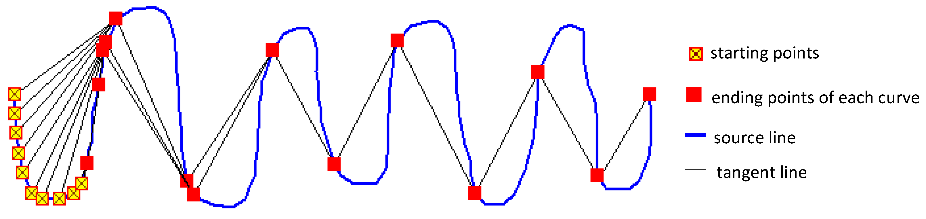
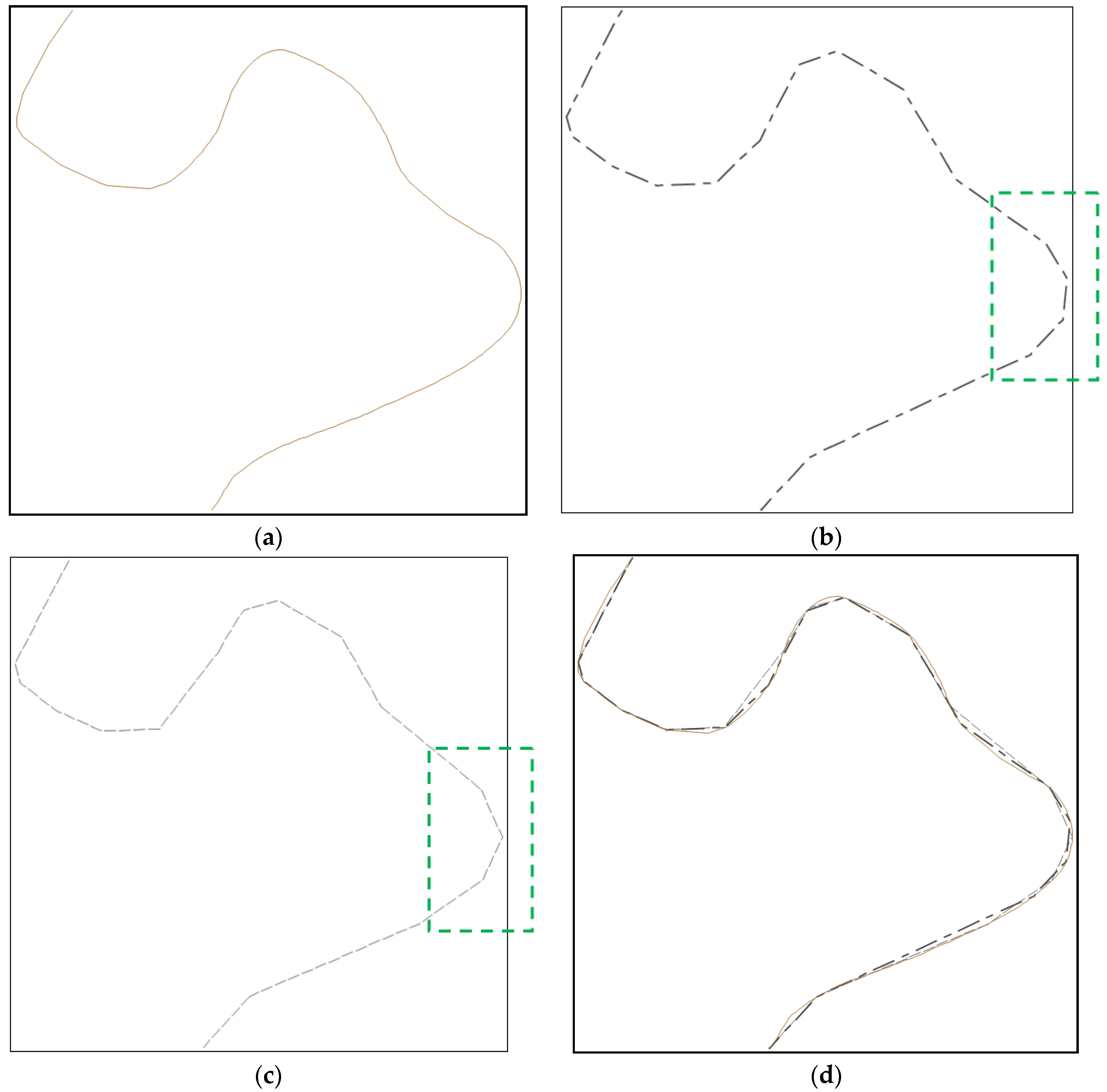
To demonstrate the “stableness nature” of the ODC method, it is necessary to compare and analyze the final division results when different starting points are selected. A large number of experiments demonstrate that choosing different starting points will lead to nearly the same division results although the first several divided curves will be a bit different.

For example, as depicted by Figure 6, when different starting points are selected, only the first three divided curves are slightly different while all the others are same, which shows that the ODC method provides generic and robust performance for line divisions due to the fact that the selection of the starting points almost has no influence on the overall final division results. For contour lines, this kind of generic nature is important because the contour lines are normally closed, which means the natural starting points do not exist at all. Certainly, if one cartographic line is not enclosed, then it is better to start the division process from one of the endpoints of the line.

3. Methodologies for Line Simplification

3.1. Classification of the Divided Curves

In the proposed line-simplification approach, the curves divided by the ODC method will be classified into different groups for further processing according to both of their shapes and sizes.

3.1.1. Identification of the U and V-shaped Curves

In terms of polylines’ shape, the curves resulted from the division can be categorized into U or V-shaped. The curves in different shapes should trigger different strategies for the line simplification.

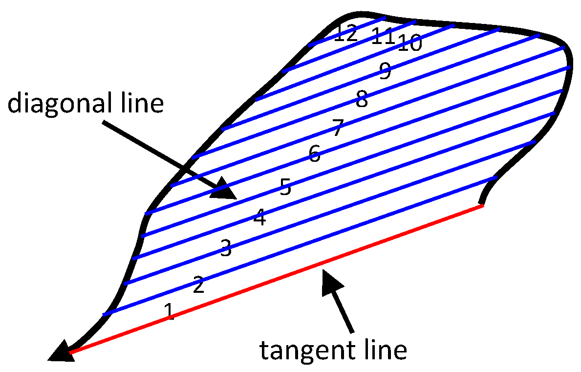
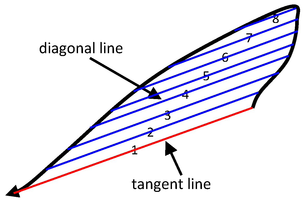
The process to identify the U or V-shaped curves is illustrated in Figure 7 and Figure 8, where Figure 7 depicts a typical U-shaped curve and Figure 8 depicts a typical V-shaped curve. First, along the direction of the tangent line, the inner space of each curve is divided by a set of diagonal lines parallel to the tangent line. Then the lengths of all the diagonal lines are measured and recorded. 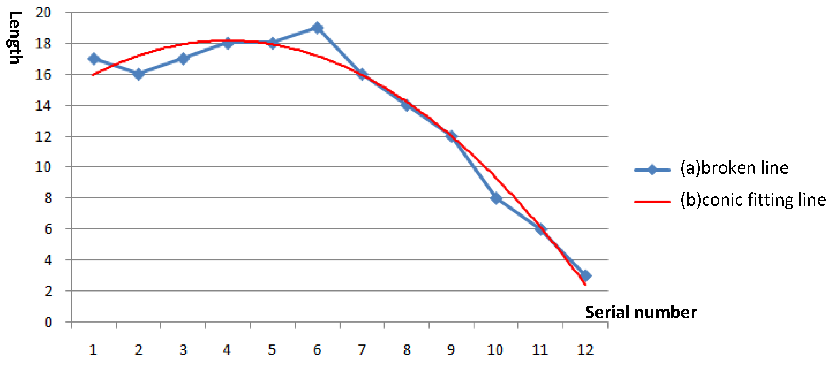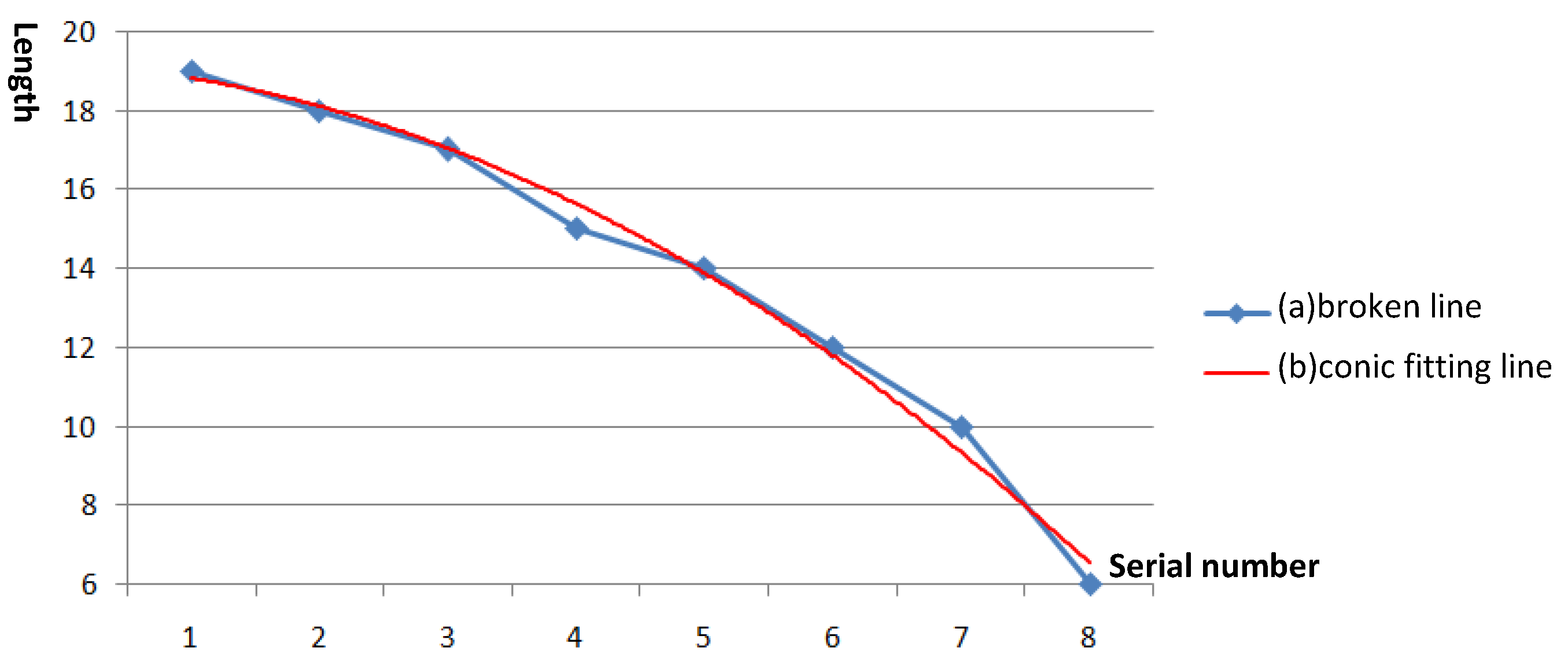Let x represent the serial number and y the length of the diagonal lines, two broken-line graphs can be drawn to respectively represent the changing trends of the diagonal lines of the U and V-shaped curves (see Figure 9a and Figure 10a).

y = −0.2468 x² + 1.9770 x + 14.1818

(1)

y = −0.1726 x² − 0.1964 x + 19.1607

(2)

Based on the fitting algorithm of Least Square for Curves, the broken-line graphs of Figure 9a and Figure 10a can be converted to the conics defined by Formulas (1) and (2), see the corresponding graphs in Figure 9b and Figure 10b.

As illustrated by Figure 9b and Figure 10b, the changing trends of the diagonal lines’ lengths of the U and V-shaped curves are different from each other—the fitting conic of the U-shaped curve has a larger curvature than that of the V-shaped curve. The average curvature of the fitting conics is used to differentiate the U and V-shaped curves. See details below:

Setting the standard conic function as in Formula (3), the curvature at a certain point x_i can be represented by (x_i) in Formula (4).

$$y=a{x}^2+bx+c$$

(3)

$$\rho (x_i)=\frac{\left|y_i^{″}\right|}{{(1+{y_i^{\prime }}^2)}^{3/2}}$$

(4)

where, y′ and y″ represent the first and second -order derivatives of y.

Then, Formula (5) can be employed to calculate their average curvatures:

$$\overline{\rho }={\displaystyle \sum _{i=1}^n\frac{\rho (x_i)}{n}={\displaystyle \sum _{i=1}^n\frac{\left|y_i^{″}\right|}{n{(1+{y_i^{\prime }}^2)}^{3/2}}}}$$

(5)

where, n is the number of diagonal lines, $i,n\in N$.

As $y_i^{\prime }=2ax+b$ and $y_i^{″}=2a$, Formula (5) can be replaced by Formula (6):

$$\overline{\rho }={\displaystyle \sum _{i=1}^n\frac{\left|2a\right|}{n{(1+{(2a{x}_i+b)}^2)}^{3/2}}}$$

(6)

According to Formula (6), the average curvature $\overline{\rho }$ for the U and V-shaped curves can be respectively calculated as follows:

${\overline{\rho }}_{standard-U}$ = 0.153356 (a = −0.2468 and b = 1.9770, ref. Formula (1) of the U-Shaped curve); and

${\overline{\rho }}_{standard-V}$ = 0.075298 (a = −0.172 and b = −0.1964, ref. Formula (2) of the V-Shaped curve).

It is obvious that ${\overline{\rho }}_{standard-U}$ is larger than ${\overline{\rho }}_{standard-V}$.

After a large number of experiments, it is found that curves with the $\overline{\rho }$ larger than 0.1 can be regarded as U-shaped while those with small than or equal to 0.1 (viz. $\overline{\rho }\le 0.1$) can be classified as V-shaped.

3.1.2. Methods to Differentiate the Large, Small and Minimum Curves

In order to get more reasonable simplification results, the curves with different sizes should be treated differently as well. In the proposed approach, one curve can be classified as large, small or minimum following the method discussed below.

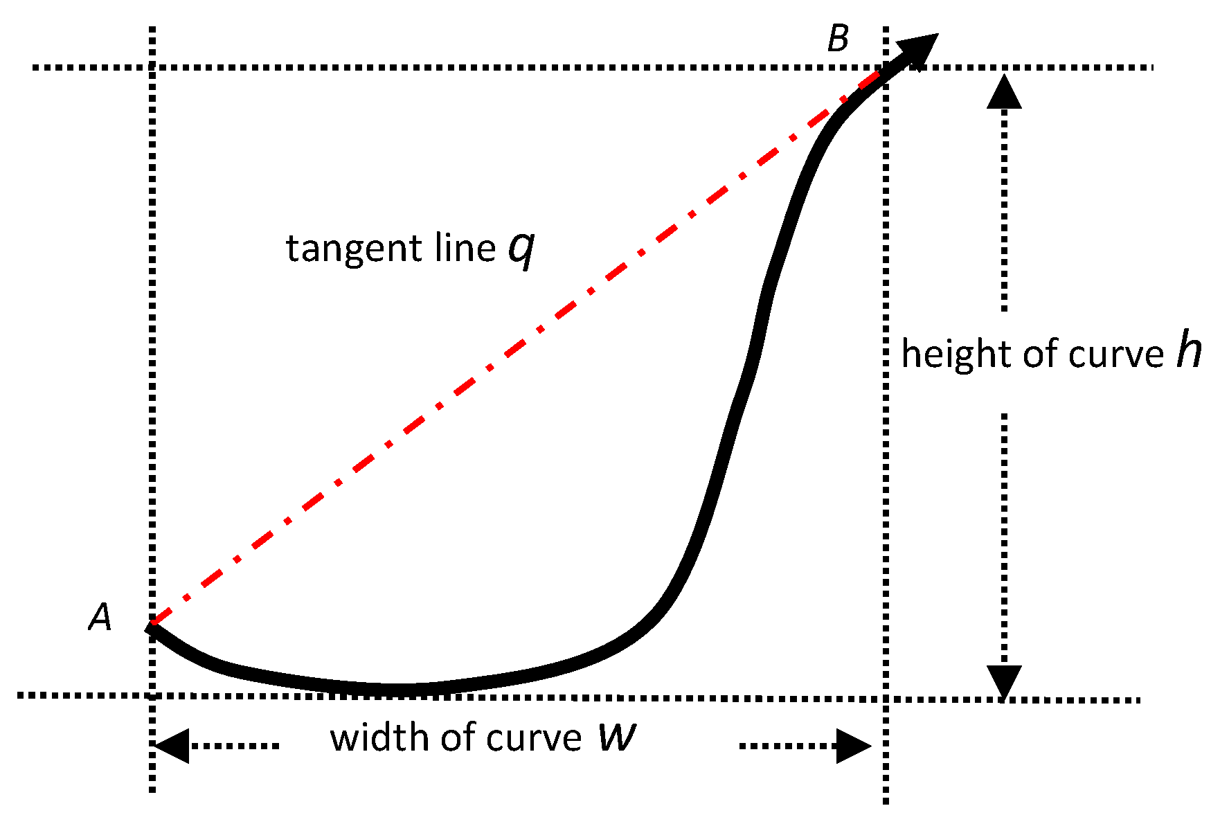
Figure 11 shows that the size of a curve is mainly determined by its height h and width w. As illustrated by

Table 1. Criteria values of [h₁, h₂, w₁, w₂] to determine the sizes of curves.

	Size	Large Curve	Small Curve	Minimum Curve
Parameters
h		>h1	(h2, h1)	<h2
w		>w1	(w2, w1)	<w2

, if h is larger than a certain threshold h₁ or w is larger than a certain threshold w₁, the curve should be treated as ‘large’; otherwise it will be treated as ‘small’ or ‘minimum’ (ref. Table 1). In the process of real-world data production, however, it could be complicated and take a lot of precious computing resources to calculate h and w.

Considering that the length of the tangent q is positively correlated with h and w and can be roughly calculated by $\mathrm{q}\approx \sqrt{{(h/2)}^2+w^2}$, the criteria based on q can be employed to differentiate the size of one curve. As illustrated by

Table 2. Criteria values of (q__small, q__large) to determine the sizes of curves.

	Size	Large Curve	Small Curve	Minimum Curve
Parameters
q		>qL	(qS, qL)	<qS

, if q is larger than a certain threshold q_L, the curve should be treated as ‘large’; otherwise it will be treated as ‘small’ (q_s ≤ q ≤ q_L) or ‘minimum’ (q < q_s), where assigning proper values to q_s and q_L becomes one of the pivotal issues to ensure the quality of the final results.

Assuming that all of the cartographic lines to be simplified have been divided into n curves in total and all these curves have been sorted based on their tangents’ lengths (viz. q) from small to large as $\{q_1,q_2,\dots ,q_j,\dots q_n\}$, the thresholds of q_s and q_L can be experimentally settled according to the Formulas (7)~(9):

$$j=n\times (1-\sqrt{\raisebox{1ex}{$Scal{e}_S$}\!\left/ \!\raisebox{-1ex}{$Scal{e}_T$}\right.}$$

(7)

q_s = q_j

(8)

q_L = q_s + (q_n − q_s)/K

(9)

where, n represents the number of all of the curves;

$Scal{e}_S$ represents the initial scale of the source data;

$Scal{e}_T$ represents the target scale after data generalization;

j is a natural number calculated according the round method;

K is a natural number, which can be settled between 3 and 10 experimentally.

It is not hard to find that (i) Formula (7), viz. the square root law [28], which has been widely used in the process of data ”selection”, is employed to identify the threshold of q_s; and (ii) the larger the K is, the smaller the q_L is and the more curves will maintain their “large” characteristic. The large curve will remain as “large” after data simplification (ref. the Section 3.2.1 and Section 3.2.2) and thus it can keep more original geometric characteristics (e.g., shape, orientation, etc.) of the whole cartographic line.

3.2. Customized Simplification Methods for Different Kinds of Curves

In this article, the Douglas-Peucker (DP) algorithm is employed as the “basis” to simplify the curves. The standard DP algorithm can be characterized by the following steps: (a) connect the starting and end points of the polyline with a straight line; (b) calculate distances of all the points to the straight line and find out the maximum distance value d_max; (c) compare with d_max and a given threshold D (viz. tolerance distance). If d_max < D, delete all points between the starting point and the end point of the polyline; otherwise, divide the whole polyline into two parts according to the point having d_max and reuse the same method to the divided parts repeatedly [13,29].

Clearly, the standard DP algorithm can sometimes result in sharp bends and destroy the crucial geometric characteristic after data simplification. With the aid of the ODC method, different kinds of curves resulted from the division will be dealt with differently which can enhance the simplification performance dramatically, especially for contour lines (see the experiments in Section 4). In fact, the proposed simplification approach does not necessarily make use of the DP algorithm, i.e., other popular algorithms for line simplifications (e.g., the VW algorithm) can be employed here as well.

As mentioned above, the curves generated by the ODC method could be categorized into different groups according to their shapes and sizes. Different kinds of curves, however, will follow different disciplines in the process of line simplification (ref. Section 3.2.1, Section 3.2.2, Section 3.2.3 and Section 3.2.4).

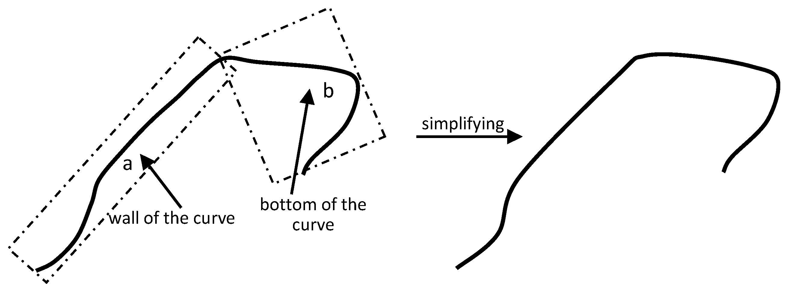
3.2.1. Simplification of the Large U-Shaped Curves

In the process of simplifying the large U-shaped curves, two requirements should be satisfied: one is to retain the whole size of the curves and the other is to ensure that U-shaped curves be still U-shaped after being simplified. To accomplish these two requirements, the wall of the curve can be simplified to a large extent (see the example of “a” in Figure 12), while on its bottom only small sinuosity should be simplified (see the example of “b” in Figure 12).

According to Formulas (10) and (11), this result can be obtained by the adjustment of the tolerance distance of the DP algorithm.

$$D_{bottom-largeU}=D$$

(10)

$$D_{wall-largeU}=2.0\times D$$

(11)

where, “D” represent the “tolerance distance” settled for the whole simplification approach; “2.0” is an empirical coefficient.

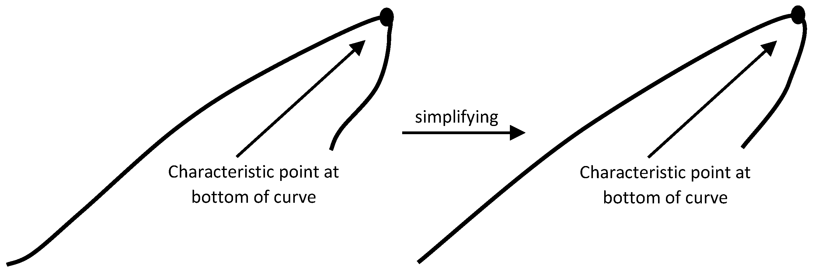
3.2.2. Simplification of the Large V-Shaped Curves

Comparing to U-shaped curves, the geometric characteristics of V-shaped curve can be easily kept because it is almost not possible to convert the V-shape curves to U-shape unless the characteristic points on the cusp are removed. Therefore, as long as the characteristic points on the cusp are preserved, large V-shaped curves can be simplified adequately, see the example in Figure 13. For the V-shaped curves, the tolerance distance of the DP-algorithm can be settled as “1.5 × D”, where “1.5” is an empirical coefficient.

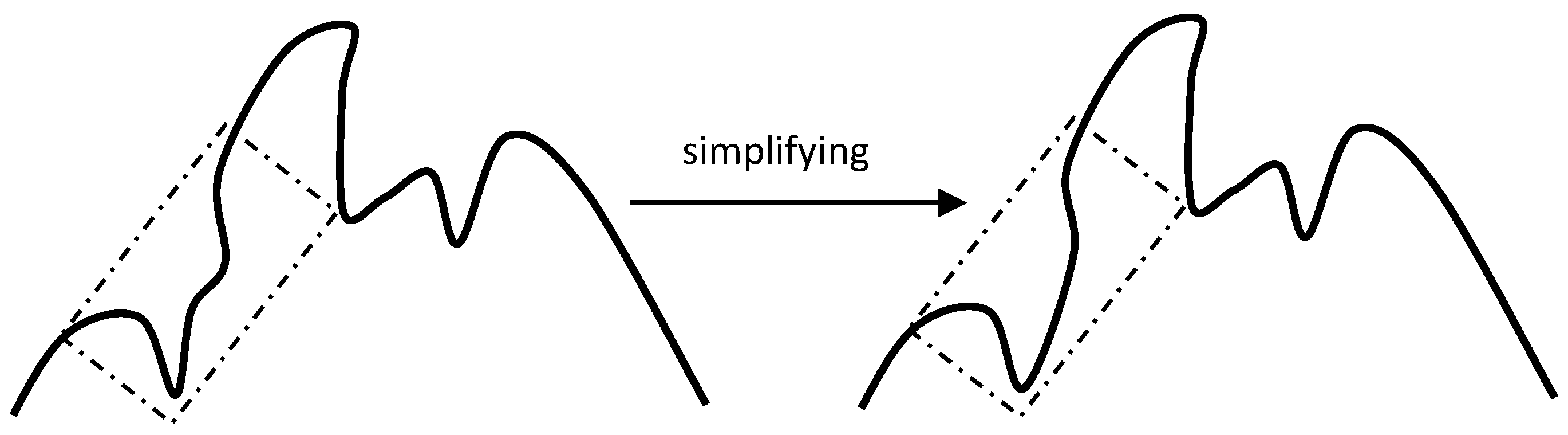
3.2.3. Simplification of the Small U and V-Shaped Curves

As small curves (incl. U and V-shaped) do not have prominent influences on the holistic shape of the whole cartographic line to be simplified, they can be simplified with the standard DP algorithm without any further constraint (see the examples in the dot-dashed box of Figure 14), where the “tolerance distance” of the DP algorithm is equal to “D”.

3.2.4. Simplification of the Minimum U and V-Shaped Curves

Curves with minimum size, no matter they are U or V-shaped, have nearly no influence on the holistic shape of the whole cartographic line to be simplified. Therefore, the minimum curves are directly eliminated in the proposed approach, where the ‘elimination of the curve’ refers to ‘connecting the starting and ending points and removing all the other turning points of the curve in between’ (see the examples in Figure 15).

3.3. Schematic Process of the Overall Line Simplification

Let l represent the curve to be simplified and f(l) represent the simplification operation conducted on l. If l has been successfully simplified by f(l), which indicates that the shape of l has been changed, then the value of f(l) is set to 1 (viz. f(l) = 1); otherwise f(l) = 0. With such a definition, the proposed approach for the line-simplification can be illustrated by the following iteratively operated eight steps.

Step 1: According to the ODC method, divide the cartographic line to be simplified into n curves, denoted as {l₁, l₂, …, l_i, … l_n} ($i,n\in N, 1\le i\le n$).

Step 2: Set i = 0 and start the processes of line simplification.

Step 3: Judge whether l_i is U-shaped or V-shaped based on the criteria defined in Section 3.2.1.

Step 4: Judge whether l_i is large, small or minimum based on the criteria defined in Section 3.2.2.

Step 5: Implement different methods f(l) to simplify the l_i according to its size and shape (viz. large V-shaped, large U-shaped, small or minimum) following the rules written in Section 3.2.1, Section 3.2.2, Section 3.2.3 and Section 3.2.4.

Step 6: If f(l_i) = 1 (viz. l_i’ ≠ l_i), replace l_i by l_i’ and return to step 1 for the re-execution of the ODC-division and the line simplification.

Step 7: If f(l_i) = 0 (viz. l_i’ = l_i) and i < n, let i = i + 1 and return to step 3.

Step 8: If f(l_i) = 0 (viz. l_i’ = l_i) and i = n, stop the iteration and terminate the simplification process.

As mentioned in Step 5, the case where f(l_i) = 1 will always lead to a re-division of the whole cartographic line as well as the re-execution of the line-simplification process. The reason is that the change of l_i will influence the geometric/topologic characteristics of its neighbours and therefore a re-division becomes necessitated for better simplification results.

4. Experiments and Evaluations

4.1. Comparison of Different Division Methods on the Same Cartographic Line

As illustrated in

Table 3. Comparison of the different simplified results of contour lines.

	Parameters	Source Line	DP-Algorithm (D = 40 m)	DP-Algorithm (D = 80 m)	DP-Algorithm (D = 120 m)	DP-Algorithm (D = 160 m)	DP-Algorithm (D = 200 m)	DP-Algorithm (D = 10,000 m)
Division Methods
Division at minimum of curvature—from left to right (Row-A)
		620 points	53 points	35 points	31 points	18 points	17 points	9 points
Division at minimum of curvature—from right to left (Row-B)
		620 points	53 points	31 points	29 points	20 points	17 points	9 points
Segmentation with ODC method—from top to bottom (Row-C)
		620 points	182 points	165 points	142 points	123 points	103 points	42 points
Segmentation with ODC method—from bottom to top (Row-D)
		620 points	197 points	183 points	152 points	134 points	94 points	37 points

, the same cartographic line has been divided by different methods as well as in different directions. Then all of the divided curves (incl. Row A–Row D) are simplified with the DP algorithm along with a series of stepwise increased parameter “D” (viz. 40, 80, 120, 160, 200 and 10,000 m).

In Row-A and B, the cartographic lines are respectively divided at the points of “peak” and “valley” (viz. the orthographic divisions from different directions). In Row-C and D, however, the cartographic line is divided based on the ODC method starting from different points and with opposite directions—one is from top to down and the other is bottom to up, where the blue points represent the dividing points in the last iteration of the ODC segmentation.

Comparing to the divisions at “peaks” or “valleys”, the ODC method has two advantages:

(1)

The ODC method is more stable

Initially, the cartographic line consists of 620 shape points. In Row-A and B, the cartographic lines have been dramatically simplified from 620 shape points to 53 shape points in the case of “D = 40”. After that, viz. when the parameter “D” is increased from 80 to 10,000, the simplified efficiency becomes much weaker. In Row-C and D, the change trends of the simplified cartographic lines are much smoother, which demonstrates that the ODC method is not sensitive to the parameter setting and therefore reveals the characteristic of stableness for the purpose of line simplification. Moreover, along with the increase of the parameter “D”, unexpected distortions occur on the sinuosity in Row-B, while the bending characteristics are always well maintained with the ODC method (see Row-C and D in Table 3).

(2)

The ODC method is more robust

As illustrated in the last column of Row A and Row B in Table 3, the quite different simplified results have been achieved when the cartographic line is divided in different ways—one is divided at ”peak” and the other is divided at “bottom”. With the ODC method, the simplified results tend to be the same even though the cartographic line has been divided using different starting points and following different directions (ref. the last column of Row C and D). Therefore, the ODC method is very robust for the purpose of line simplification. Moreover, the ODC method also helps to preserve the geometric and topologic characteristics of the initial cartographic lines in the process of data simplification (see Row-C and D in Table 3).

In addition, due to fact that the ODC method is iteratively processed and the curves generated by the ODC method are dealt with in different ways according to their specific shapes (viz. U and V-shaped) and sizes (viz. large, small, minimum) by the customized simplification rules, the proposed approach based on the ODC method demonstrates better simplification performances with respect to geometric accuracy comparing to traditional methods.

Figure 16, for instance, compares the simplification results based on the same cartographic line (ref. Figure 16a), where Figure 16b illustrates the simplified result using the ODC method and Figure 16c illustrates the simplified result with divisions at the inflection points. Although both of the simplified lines have been compressed to the same amount of shape points, Figure 16b keeps more geometric characteristics of the original cartographic line than Figure 16c. For instance, the sinuosity in the middle-right part of Figure 16a remains U-shaped in Figure 16b (see the area in the green dashed box), while it becomes V-shaped in Figure 16c (see the area in the green dashed box). Moreover, the simplified line based on the ODC method fits the shape and location of the initial cartographic line better (see the comparison in Figure 16d).

4.2. Evaluation of the Overall Performance of the Proposed Simplification Algorithm

Figure 17 illustrates a number of contour lines to be simplified. After 0.2 s. on a normal personal computer (CPU: Intel Core i7 2.80 Hz, 4G physical memory), the contour lines have been adequately simplified from 72723 shape points to 17591 shape points. The compression rate reaches (1-17591/72723) × 100% = 75.8%. Figure 18 demonstrates that with the proposed ODC method and simplification approach, most of the geometric and topological correctness of the contour lines have been maintained – the simplified lines kept smooth and undistorted after the simplification process. With the traditional division method, however, the U-shaped curves could be changed to V-shaped and vice versa. In addition, issues such as improper distortions and topologic errors (e.g., self-intersections) could occur frequently after the simplification process, see example in Figure 19.

As mentioned earlier (ref. Section 3.2), our proposed approach applies different disciplines and criteria to the curves in different groups of “large U-shaped”, “large V-shaped”, “small U and V-shaped” and “minimum U and V-shaped” when processing line simplification. In this way, the simplified results will almost remain unchanged when parameter “D” increases to a certain level. In Figure 18, for instance, the contour lines will not be further simplified significantly when parameter “D” becomes greater than 40, which avoids a number of simplification errors especially in the case that improper parameters have been assigned by unskillful users. This is also a key advantage of the proposed approach in comparison to some other existing simplification methods.

To further demonstrate the advantages of the proposed simplification approach, a series of simplification results generated by different methods are compared in Figure 20 to Figure 21.

For instance, Figure 20a illustrates the simplification results based on the traditional method, while Figure 20b illustrates the simplification results based on the ODC method. After line simplification, 1580 and 1518 shape points are remained in Figure 20a,b respectively. Although their compression rates are at the same level, Figure 20b demonstrates better simplification results due to the fact that (a) the simplified contour lines in Figure 20b are smoother than those in Figure 20a; (b) the U-shaped curves have been changed to V-shaped and vice versa in Figure 20a, while such unexpected distortions have been primarily avoided in Figure 20b; and (c) the transformation of the simplified contour lines in Figure 20b are smaller than those in Figure 20a in terms of shape and location, which reduces a number of topologic problems like “intersections between neighbored contour lines” (see the comparison in the area enlarged by the dashed box at the lower-left corner of Figure 20a,b).

The proposed ODC method and the traditional method demonstrate more prominent differences when the contour lines are further simplified (see Figure 21). For instance, more topologic issues of “intersections” have occurred when the contour lines are simplified by the traditional method (see the areas enlarged by the two dashed boxes in Figure 21a). With the ODC method, however, the topologic conditions are maintained properly (see the areas enlarged by the two dashed boxes in Figure 21b).

Besides the example illustrated above, the proposed approach has been implemented on a number of experiments to simplify the contour lines in the basin of Yangtze River of China. The overall simplified results are quite satisfactory.

Worth mentioning is that the proposed simplification approach can still be further improved even with significantly positive performance on simplifying contour lines in various large test areas. In the process of data simplification, for instance, the current approach merely calculates the geometric and topologic characteristics of an isolate contour line, i.e., the shape and/or locations of its neighbors are not considered. Therefore, the undesirable conditions such as the “intersection between different contour lines” cannot be completely avoided when the neighboring contour lines are located too close, even though the proposed ODC method can dramatically reduce the probability of generating such topologic problems (ref. Figure 20 and Figure 21). In the future, two possible ways can be tried to avoid the potential topologic errors for line simplification. One way is to integrate transformation constraints during the line simplification process; the other is to operate a post-processing procedure to recover the initial topologic relationships in areas where the contour lines are densely distributed (e.g., at the positions of precipices).

5. Conclusions

In this article, a new line-simplification approach based on the Oblique-Dividing-Curve (ODC) method has been proposed. With this approach, one cartographic line to be simplified can be firstly divided into a chain of shorter curves by the ODC method. According to their geometric characteristics regarding shapes and sizes, the curves are categorized into four groups: “large U-shaped”, “large V-shaped”, “small” and “minimum”. Then, the curves in different groups trigger different rules and criteria for line simplification.

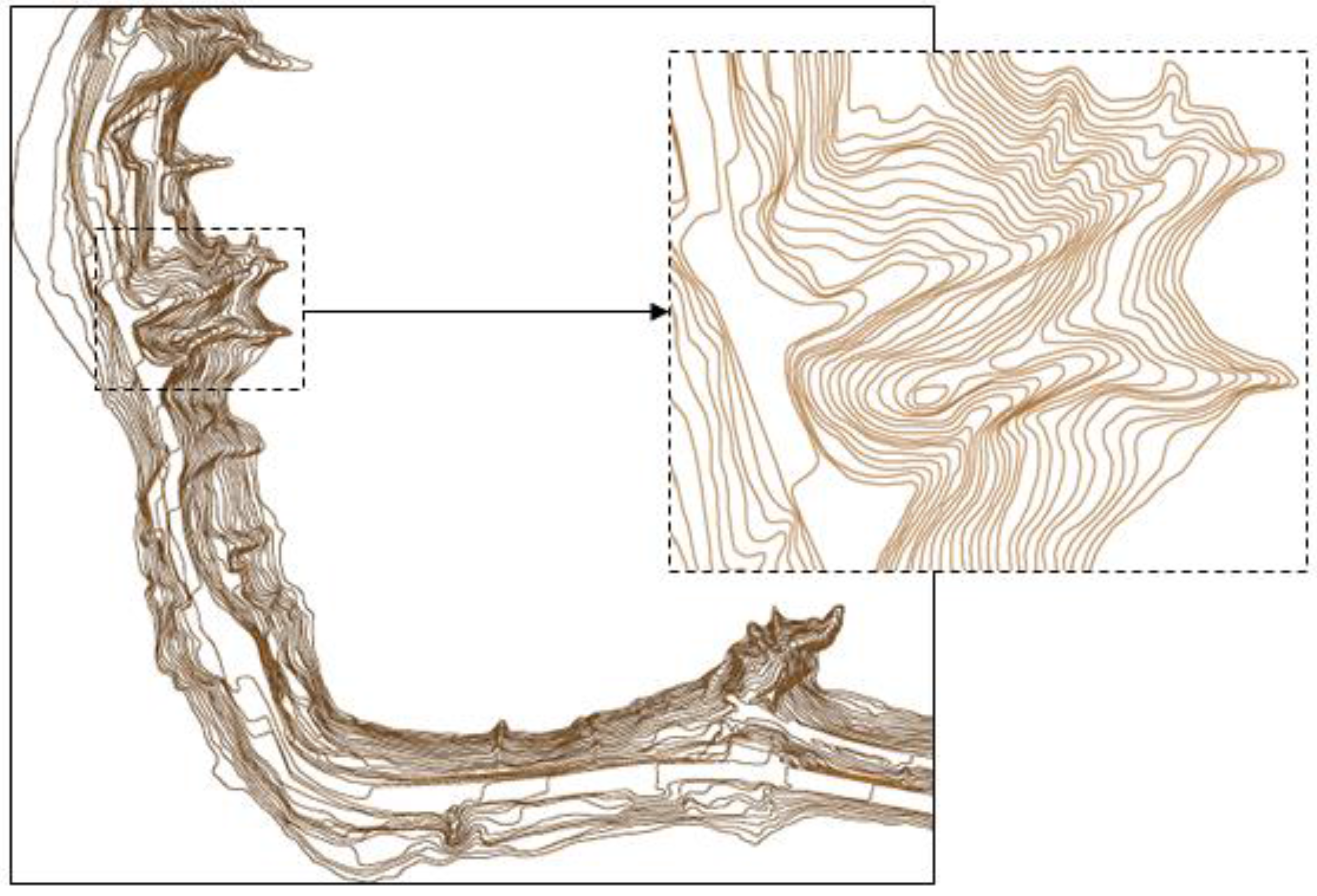
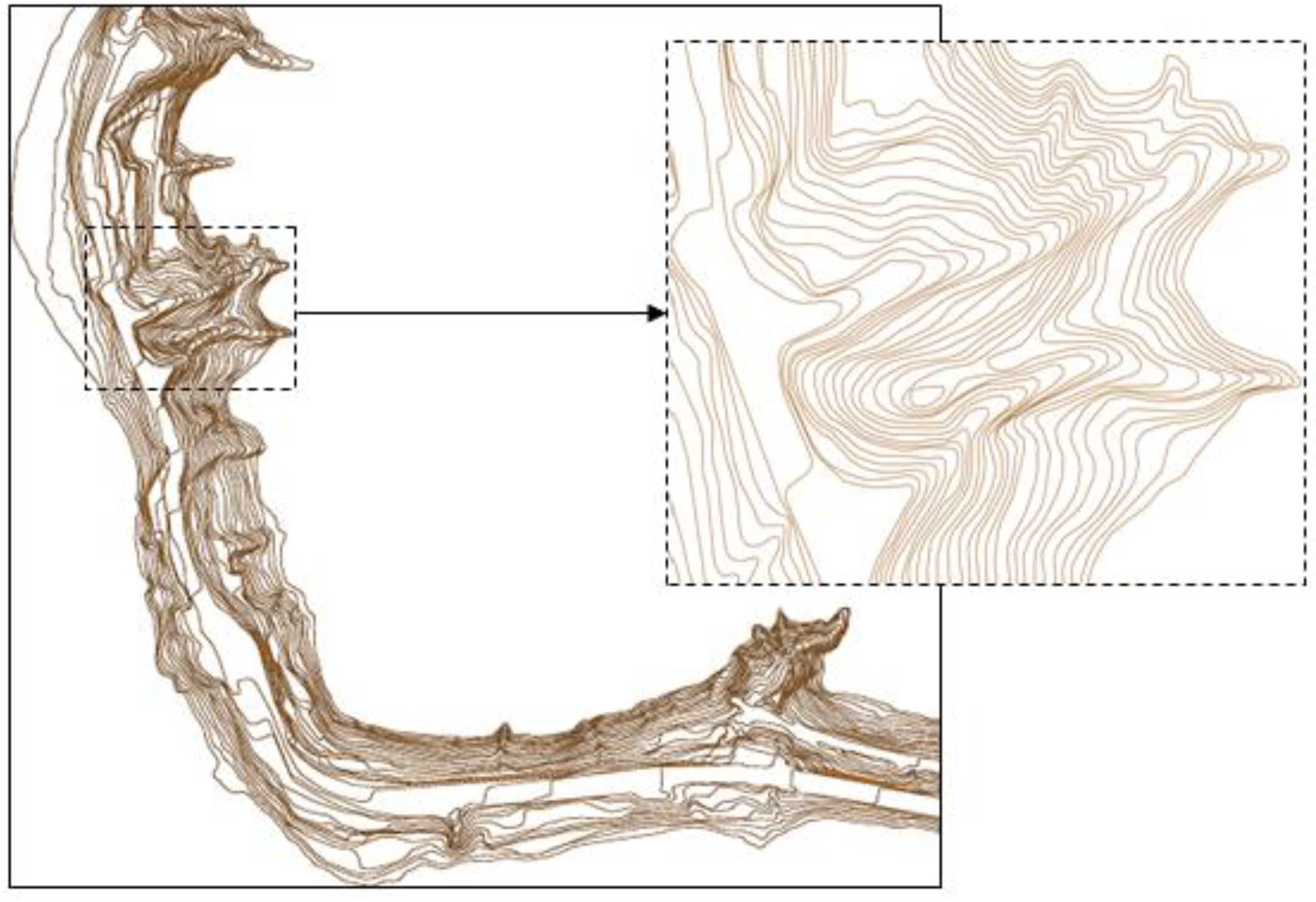
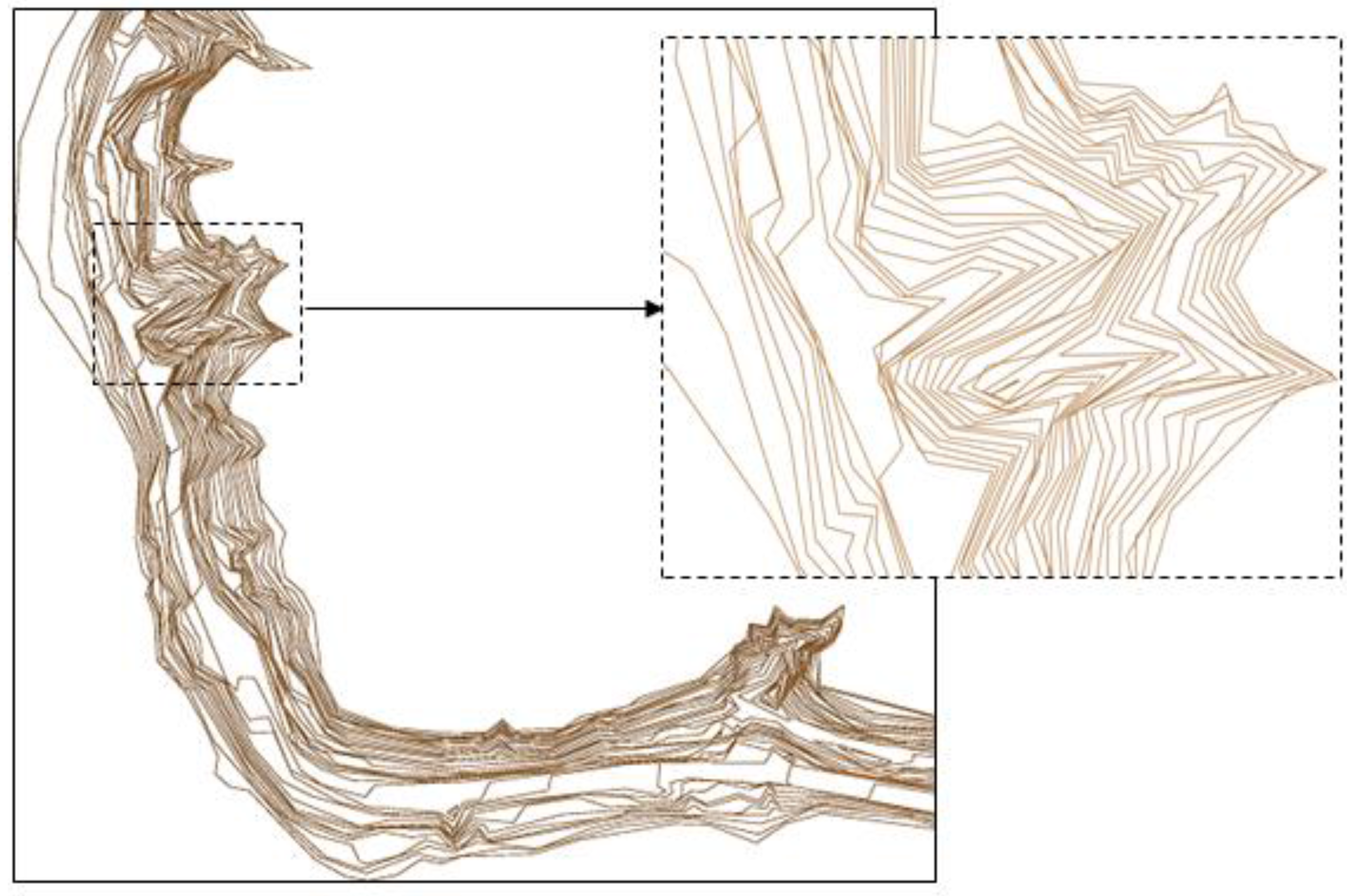
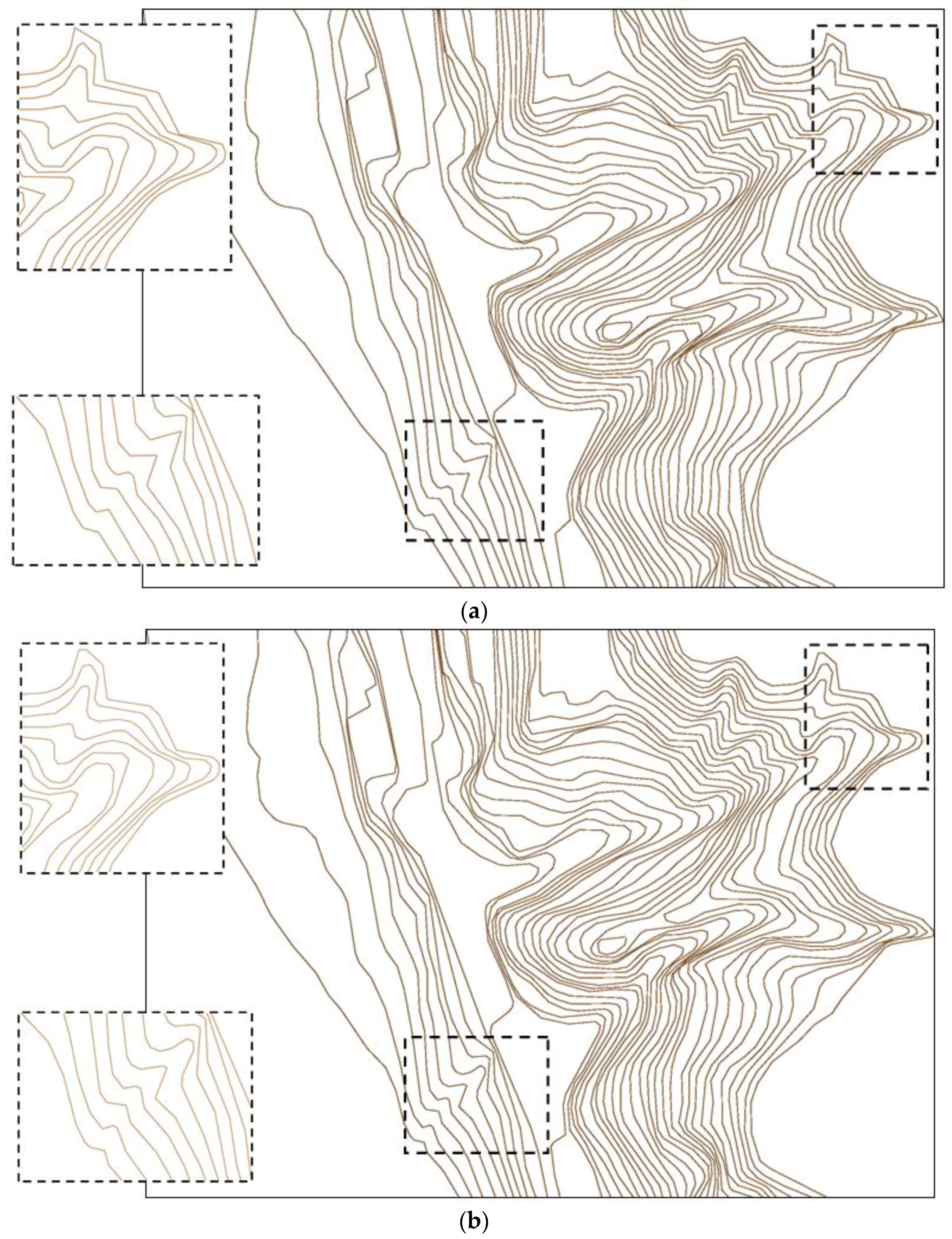
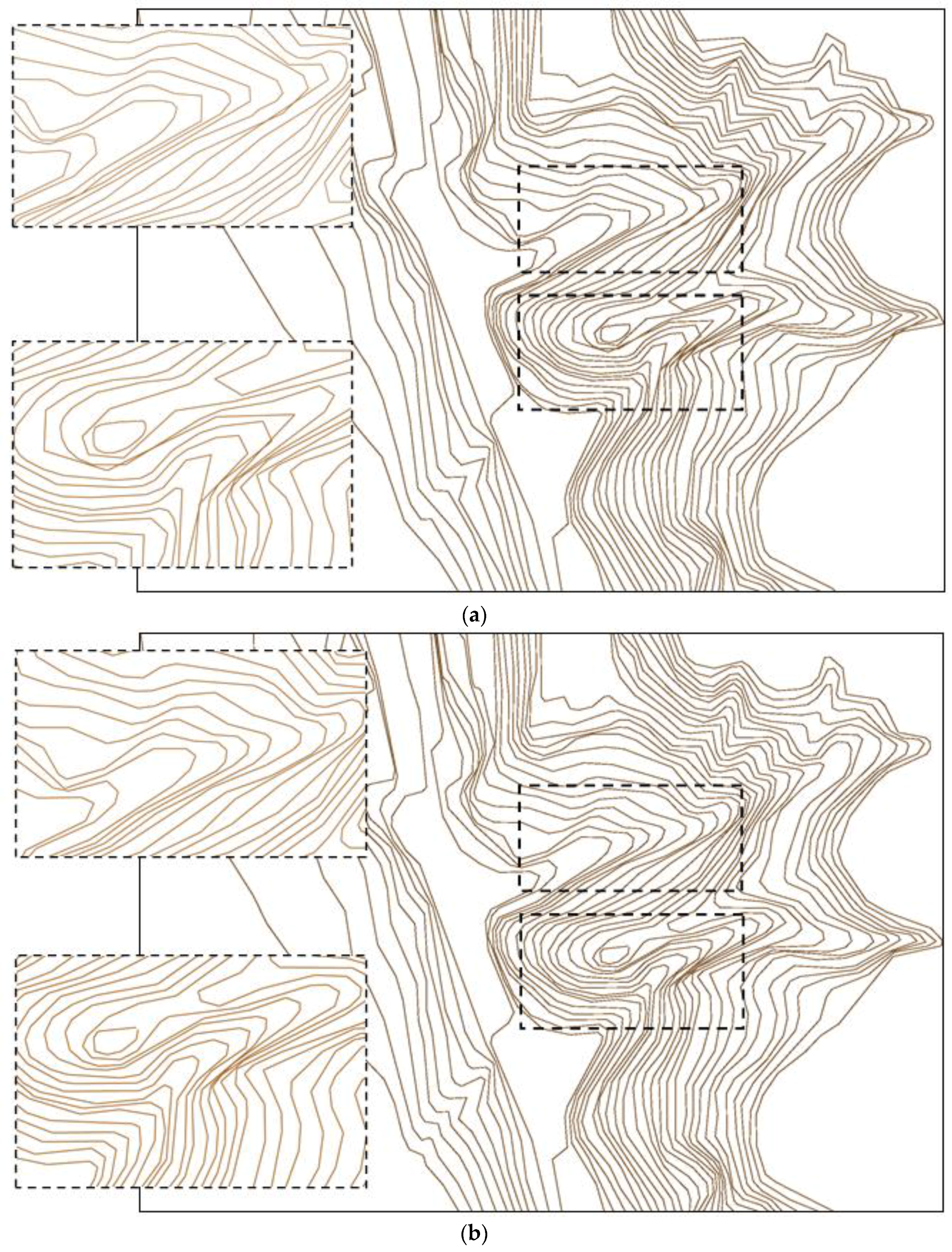
Supported by the iteratively operated ODC divisions and the customized simplification strategies for different curve groups, the proposed approach is able to handle geometric and topologic characteristics in a holistic environment and provide considerably improved line simplification performance in terms of (a) stability—the simplified lines change smoothly along with the increase of the parameter “D”. That is, the approach is not sensitive to the parameterizations; (b) robustness—the simplified results will not be significantly influenced when the process starts from different starting points and/or in opposite directions; (c) geometric accuracy—even though the cartographic lines have been simplified to a great extent (e.g., in case that the compression rate reaches 75.8%), the proposed approach can adequately maintain the general characteristics in terms of the position, orientation and shape (U- or V-shape) of the cartographic lines regardless how the parameters are set. This “accurate” nature allows the simplified contour lines to be merely slightly transformed based on the initial ones, which helps to reduce the probability of topologic issues of “intersection”. Moreover, the computing speed is acceptable. For instance, it only takes 0.2 s to accomplish the simplification process of reducing the number of the shape points from 72,723 to 17,591, which means 275,660 reduced points per second, on a common personal computer. Rather than a significant prototype, the proposed approach has already been utilized for the real-world data productions of contour lines simplification on more than 6400 topographic maps with a total area of 640,000 square kilometers (=10 km × 10 km × 6400) in the basin of Yangtze River of China. The automatic simplification results are indeed satisfactory.

Besides the contour lines, the same simplification method is now being experimented on various types of hydrographic lines, coast lines, administrative boundaries, etc. Clearly, it is not enough to merely implement the line simplification for the data generalization in many cases. In the future, the proposed line-simplification approach will be further researched so that it can work together with other operators of data generalization.