Automatic Scaling Hadoop in the Cloud for Efficient Process of Big Geospatial Data

Abstract

Efficient processing of big geospatial data is crucial for tackling global and regional challenges such as climate change and natural disasters, but it is challenging not only due to the massive data volume but also due to the intrinsic complexity and high dimensions of the geospatial datasets. While traditional computing infrastructure does not scale well with the rapidly increasing data volume, Hadoop has attracted increasing attention in geoscience communities for handling big geospatial data. Recently, many studies were carried out to investigate adopting Hadoop for processing big geospatial data, but how to adjust the computing resources to efficiently handle the dynamic geoprocessing workload was barely explored. To bridge this gap, we propose a novel framework to automatically scale the Hadoop cluster in the cloud environment to allocate the right amount of computing resources based on the dynamic geoprocessing workload. The framework and auto-scaling algorithms are introduced, and a prototype system was developed to demonstrate the feasibility and efficiency of the proposed scaling mechanism using Digital Elevation Model (DEM) interpolation as an example. Experimental results show that this auto-scaling framework could (1) significantly reduce the computing resource utilization (by 80% in our example) while delivering similar performance as a full-powered cluster; and (2) effectively handle the spike processing workload by automatically increasing the computing resources to ensure the processing is finished within an acceptable time. Such an auto-scaling approach provides a valuable reference to optimize the performance of geospatial applications to address data- and computational-intensity challenges in GIScience in a more cost-efficient manner.

1. Introduction

Massive volumes of geospatial data are collected at increasingly faster speeds and higher spatiotemporal resolutions with the advancement of earth observation sensors [1]. Efficiently processing big geospatial data is essential for tackling global and regional challenges such as climate change and natural disasters [2,3]. Decision support for emergency response, for example, can only be best performed when integrating and processing a large amount of geospatial data in a timely fashion because one-second early warning or alert may help save more lives [4,5].

However, efficient processing of big geospatial data is challenging not only due to the massive data volume but also due to the intrinsic complexity and high dimensions of the geospatial datasets [6]. For example, analyzing climate trends often necessitates the aggregation of information (hundreds of climatic variables) from terabytes of four-dimensional climate data spanning hundreds of years [7]. It normally takes hours or even days if such analysis was done using a single computer. DEM (Digital Elevation Model) interpolation is another good example of computing-intensive and time-consuming geospatial analysis which does not scale well with traditional computing infrastructure [8].

To accelerate geospatial data processing, distributed computing infrastructures are widely used. Hadoop, a distributed computing platform leveraging commodity computers, is gaining increasing popularity in geoscience communities, as reviewed in Section 2. While a lot of effort was put into investigating how to adapt Hadoop for processing big geospatial data (e.g., [9,10,11,12,13]), how to efficiently handle different geoprocessing workload by dynamically adjusting the amount of computing resources (number of nodes of a Hadoop cluster) was barely explored. The ability to dynamically adjust the computing resources is important because the processing workload of operational geospatial applications is rather dynamic than static [14]; for example, the data processing workload for an emergency response system (such as for wildfires, tsunami, and earthquakes) peaks during the emergency event, which requires adequate computing power to respond promptly [14,15]. Another example is that geospatial web applications/services (such as an online analytical system for interactive climate data analysis) often need to deal with different processing workloads due to the dynamic user access patterns [16,17].

One traditional solution to handle the dynamic processing workload is to preconfigure the system with “adequate” computing resources to handle peak workload. However, this is problematic because, first, it is difficult to estimate how many computing resources will be “adequate”. Second, even though we can provide adequate computing resources to handle the peak workload, this will be a huge resource waste because computing resource usage levels are often very low on average and only peak in a narrow period. Therefore, one important question remains open: how to automatically adjust the computing resources based on the dynamic workload so geospatial processing and analysis can be timely finished while minimizing resource usage (cost)?

To tackle this issue, we propose a performance-driven and cost-awareness framework to automatically scale computing resources of a Hadoop cluster based on the dynamic geospatial processing workload in a cloud environment. The contributions of this research were (1) a new storage structure is introduced to enable timely computing resources removal without incurring extra data transfer, and (2) a predictive auto-scaling algorithm is developed to more accurately calculate the amount of computing resources to add. The feasibility and efficiency framework was evaluated with a prototype system using DEM interpolation as an example. The experimental results indicate that the prototype system is able to efficiently handle the dynamic processing workload by automatically adding and removing computing resources as needed.

This paper reports the research in following manner: Section 2 reviews related work. Section 3 details the methods used in the proposed auto-scaling framework. Section 4 tests the feasibility and efficiency of the auto-scaling framework using DEM interpolation as an example, and Section 5 concludes the paper.

2. Related Work

2.1. Hadoop for Geospatial Data Processing

Leveraging a large number of computers and collocating computing resources to data storage have been widely used to ensure that the data are processed in an expeditious timeframe [18]. As an open-source implementation of the MapReduce framework [19], Hadoop is gaining increasing popularity in the Big Data era over the past years [20]. Meanwhile, many studies have been carried out to leverage Hadoop for geospatial data processing. For example, Gao et al. adapted Hadoop to construct gazetteers from volunteered big geospatial data [12]. Lin et al. leveraged Hadoop to store and process massive remote sensing images to support large concurrent user requests [21]. Krishnan et al. investigated the use of MapReduce to generate DEM by gridding the LIDAR data [22]. Li et al. utilized Hadoop MapReduce to enable penalization of big climate data processing [11,13]. Besides these problem-specific approaches focusing on solving specific problems with Hadoop, tools have also been developed to handle general geospatial data processing tasks and are being adopted in GIScience communities. For example, SpatialHadoop, an open source Hadoop extension, is designed to process huge geospatial datasets [10]. Similarly, HadoopGIS offers a scalable and high performance spatial query system over MapReduce to accelerate geospatial data analysis [23]. While these studies provide a valuable experience and guideline on how to adapt Hadoop for big geospatial data processing, how to adjust the size of the computing cluster to efficiently handle different geoprocessing workloads was not explored.

A fixed-size computing cluster has obvious drawbacks considering the dynamic workload for practical geospatial applications. First, it is neither energy nor cost-effective since the computing resources are not fully utilized when the workload is low. Second, when the workload exceeds the computing capacity, performance is degraded. To tackle these issues, Leverich et al., for example, proposed a strategy to allow the cluster to scale down when the workload is low to improve energy-efficiency [24]. Another approach for scaling down a Hadoop cluster is GreenHDFS [25], which features a multi-zone layout of hot and cold zones. The above approaches focus on removing cluster nodes, but the automation for the scaling operations is barely noted. Aiming to achieve automation, Maheshwari et al. proposed a dynamic data placement and cluster reconfiguration algorithm to turn off or on cluster nodes based on the average cluster utilization rate [26]. However, it requires data blocks stored on one node to be transferred to other nodes before node removal. Such a process is not only time-consuming but also consumes a considerable amount of network resources, especially when the data to be transferred are large. In addition, the second issue is not tackled partly due to the limitation of physical resources (purchasing and adding a physical computer to the cluster normally requires days and weeks).

2.2. Auto-Sscaling Hadoop in the Cloud

Cloud computing is a new computing paradigm with the characteristics of on-demand self-service, availability, scalability, and measured cost [27]. Cloud computing offers a potential solution for addressing the fixed size cluster challenges in that a virtual Hadoop cluster can be provisioned in a few minutes. Public cloud providers typically provide Hadoop clusters as web services allowing users to configure, provision, and terminate the cluster through a web-based interface. For example, Amazon Elastic MapReduce (EMR) [28] and Window Azure HDInsight [29] are popular cloud-based Hadoop services which enable users to quickly provision a Hadoop cluster to process large volumes of data. Once a job is finished, the users can terminate the cluster and launch another cluster for another job. However, a critical problem exists in these Hadoop services: the size of the cluster cannot be automatically adjusted based on the dynamic workload (e.g., many jobs are submitted to the same cluster in a short time). Even though some services such as Amazon EMR provide mechanisms to allow users to change the cluster size, which has to be done manually, and the burden of deciding how many machines to be removed or added is placed on the non-administrative-expert users [30].

As cloud computing and Hadoop are increasingly adopted in addressing the big data and computational problems in geospatial domains (e.g., [31,32,33,34]), how to optimize the allocated computing resources by considering the dynamic geoprocessing workload deserves investigation. However, there is little research to study dynamically scaling a Hadoop cluster in cloud environments. Romer proposed a threshold-based scaling to automatically add more nodes to the cluster based on the black box performance metrics (CPU and RAM) and predefined threshold values [35]. This scaling provisions new virtual machines when the average cluster load exceeds a threshold and then automatically configures these machines to the cluster. However, the scaling up is triggered based on the current workload. This is problematic as scaling up takes time to provision new virtual machines and configure them to the cluster (minutes to hours depending on the cloud platform). For example, it may take 10 min to provision a virtual machine (VM) on Amazon’s Elastic Compute Cloud (Amazon EC2) and add this VM to a cluster. It is likely that the workload has changed during this time period (e.g., newly added VMs are no longer needed or more VMs are required). In addition, for scaling down Romer suggested manually terminating the nodes individually. To tackle this issue, we propose a predictive auto-scaling algorithm to better estimate the required computing resources by considering the time spent on the scaling process (Section 3.3). More recently, Gandhi et al. proposed a model-driven auto-scaling solution for Hadoop clusters by estimating the dynamic resource requirements of a Hadoop job for a given execution time SLA (service-level agreement) [36]. However, to dynamically remove a slave node, the data stored in this node must be migrated to other nodes before being removed. Such a data migration process may take tens of minutes or hours depending on the data volume, making it hard to timely capture and respond to the dynamic workload. To address this issue, we propose a CoveringHDFS mechanism as elaborated in Section 3.2.

3. Methods

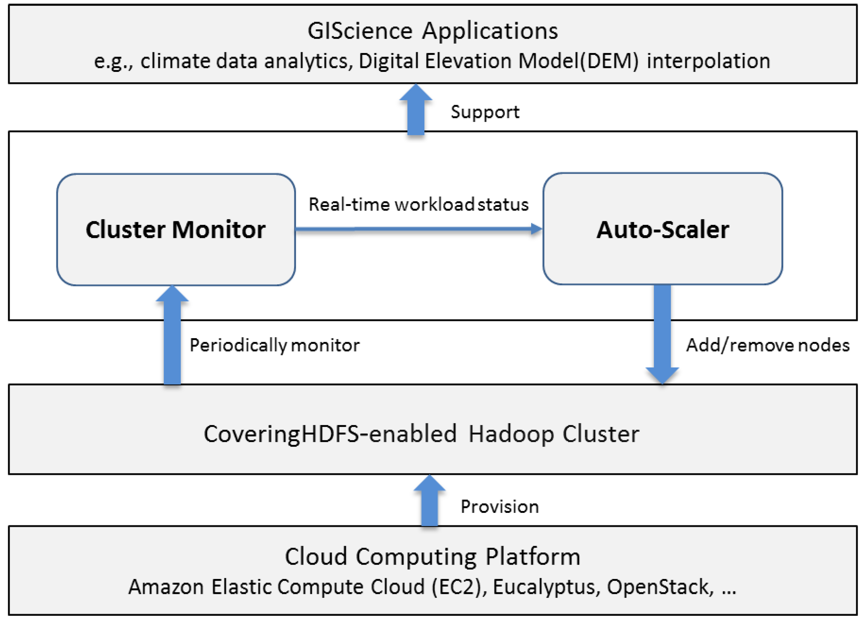
3.1. Auto-Scaling Framework

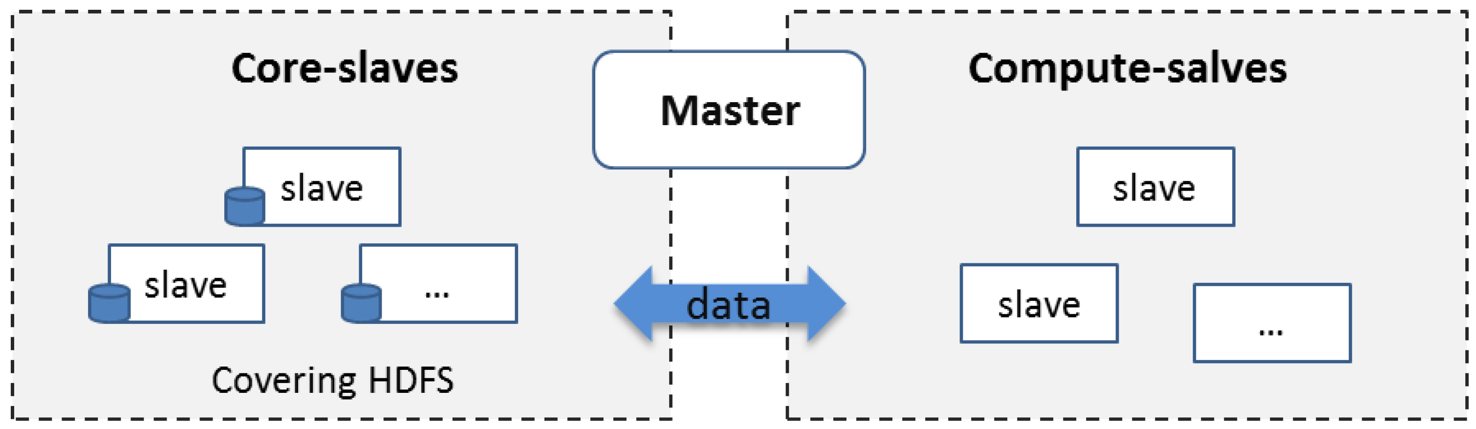
The goal of the framework is to dynamically adjust computing resources (cluster size) based on the processing workload to handle the spike requirement for computing power (e.g., to support disaster response) while minimizing resource consumption (during the low workload time period). Figure 1 illustrates the architecture of the framework, containing the following components: Cloud computing platform, CoveringHDFS-enabled Hadoop cluster, Auto-Scaler, and Cluster Monitor.

The cloud computing platform provides on-demand computing resources (virtual machines) to the framework. The cloud platform can be either a public cloud (e.g., Amazon EC2 and Microsoft Azure) or private cloud platform (e.g., Eucalyptus cloud and OpenStack).

CoveringHDFS-enabled Hadoop cluster is a virtual computing cluster consisting of a number of virtual machines provisioned by the cloud platform. This cluster is responsible for storing and processing geospatial data. CoveringHDFS (detailed in Section 3.2) enables the cluster to be promptly scaled up and down as needed.

Cluster Monitor is the driver of the auto-scaling framework, and it continuously collects the real-time workload information from the Hadoop cluster using the Hadoop API (Application Programming Interface), including running/pending jobs, running map/reduce tasks, and pending map/reduce tasks.

Auto-Scaler dynamically adds or removes computing resources using the cloud platform API (e.g., Amazon EC2 API) based on the real-time workload provided by the Cluster Monitor. If the current workload exceeds the processing power of the cluster, more computing resources (virtual machines) are added to the cluster. When the workload is relatively low, idle virtual machines are terminated. The core of Auto-Scaler is a predictive auto-scaling algorithm (detailed in Section 3.3) that determines when to trigger the scaling operation and estimates how many computing resources need to be scaled.

3.2. CoveringHDFS

By default, a Hadoop cluster uses Hadoop Distributed File System (HDFS, [37]) to store data. Data on HDFS are distributed across all data nodes (nodes that provide both storage capacity and computation) to enable data locality computation. While this storage strategy minimizes data transferring among the cluster nodes, scaling down clusters is difficult since shutting down a node incurs the risk of losing data. Hadoop provides a built-in functionality called ‘decommission’ to safely remove a node from HDFS by first transferring all data blocks from this node to the other nodes before removing it from the cluster. The time taken in decommissioning depends on the data size to be transferred (i.e., minutes, hours, days), which is intolerable for an efficient auto-scaling framework designed to timely capture and respond to a dynamic workload.

To tackle this problem, we introduce the CoveringHDFS mechanism to scale down the cluster safely and timely without losing data inspired by the covering subset concept proposed in [24]. Different from [24], instead of modifying the underlying Hadoop software, we store the data directly on a subset of the slave nodes on which the HDFS is deployed. The node consisting of CoveringHDFS are called core-slaves, and other nodes are compute-slaves. Core-slaves provide both storage and computing power, whereas compute-slaves only provide computing power. Thus, such a cloud-based computing cluster consists of three components: master node, core-slaves, and compute-slaves (Figure 2), and can have three modes: FullMode, containing core-slaves, compute-slaves, and master; CoreMode, containing core-slaves and master; and TerminateMode, the whole cluster is terminated.

By incorporating the CoveringHDFS in a cluster, idle compute-slaves can be removed instantly when the workload is low by triggering a scaling down operation. In this design, compute-slaves lose the advantage of data locality when processing the data but provide on-demand computing resources. The trade-off between data-locality and computing power is discussed in Section 4 with the experiment result.

3.3. Auto-Scaling Algorithm

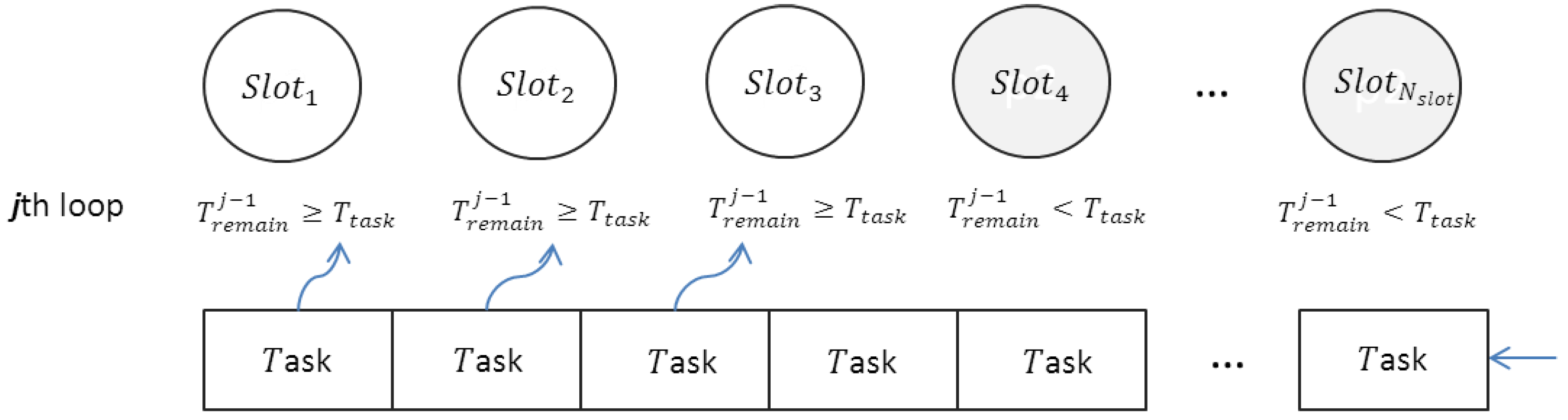
The Auto-Scaling algorithm adds compute-slaves when the workload exceeds a cluster’s computational power (e.g., jobs are waiting to be executed) and releases idle compute-slaves when the workload is low.

3.3.1. Scaling up

A MapReduce job normally contains many map tasks and one or several reduce tasks. Each slave node in the Hadoop cluster has a maximum capacity of processing map/reduce tasks in parallel which is typically determined by the slave’s number of CPU cores and memory size. Suppose each slave can support n concurrent map tasks and m reduce tasks, we can think that each slave has n map slots and m reduce slots. If the amount of map tasks (workload) exceeds that of the map slots (cluster capacity), the exceeded map tasks need to wait until free map slots are available which impairs the performance. The key for scaling up the mechanism is to estimate how many extra computing resources (compute-slaves) are required when the workload exceeds the cluster’s capacity.

Suppose that there are ten total pending map tasks at a moment $T_o$, and that each new added slave increases two map slots. One simple solution is to add five slaves so that each pending task is handled by a map slot. However, adding five slaves cannot be done instantly. For example, provisioning a medium Amazon EC2 instance with Linux OS takes approximates five minutes (until the instance is ready for connection). In this case, when the five slaves are added, there may be no pending maps, so newly added slaves have no functionality if no other jobs are submitted. Therefore, the time spent on the scaling-up process ($T_N,\mathrm{time}\mathrm{needed}\mathrm{to}\mathrm{add}N\mathrm{slaves}$) must be considered to estimate the right number of slaves to add. To this end, we introduce a predictive scaling up algorithm to estimates the workload at the time $T_o$ + $T_N$ when the scaling up process is finished. The number of slaves to be added (denoted as N) is calculated using Equation (1) as

$$N=\left[\frac{ N_{pending}-N_{finished}}{n}\right]$$

(1)

where $N_{pending}$ is the number of pending tasks at $T_o$, $N_{finished}$ is the number of pending map tasks that will be finished or become running when the scaling-up process is done, and n is the number of map slots for each added slave.

Suppose scaling up N nodes to the cluster takes $T_N$ minutes. The $N_{finished}$ is estimated as follows: for a list of processing slots ($N_{slot}$) and task queue with N map tasks, each slot has the same processing power, but each task may require a different amount of time (e.g., job types). At the moment $T_o$, each slot processes a task with the progress p. The waiting tasks are processed following the principle of first-come-first-serve. Once a slot has finished its current task, a new task is fetched from the task waiting list. This process is repeated until the time spent on each slot is $T_N$.

Based on this model, the number of pending tasks that are finished or become running during the time period $T_N$ is equal to the number of map tasks that are finished on each slot in $T_N$, which can be calculated as follows:

$$\begin{gathered} N_{finished}={\displaystyle \sum }_{i=1}^{N_{slot}}{\displaystyle \sum }_{j=1}^{T_{remain}^j>0}\min \left(\frac{T_{remain}^{j-1}}{T_{task}},1\right) \\ if\{\begin{array}{c}j=1,T_{remain}^0=T_N\text{ and }{T}_{task}=\left(1-p_i\right)*T_{i1}\\ j>1,T_{remain}^j=T_{remain}^{j-1}-T_{task}\text{ and }{T}_{task}=T_{ij}\end{array} \end{gathered}$$

(2)

where $N_{slot}$ is the number of map slots for the current cluster, $T_{remain}^j$is the time left in time period $T_N$when a node has finished j tasks (counted from time moment $T_o$), $T_{ij}$ is the time required for finishing the jth map task on the ith slot ($T_{ij}$ differs for different job types), $p_i$ is the progress of the running map task on the ith slot at $T_o$ ($0\le p_i\le 1$), and $T_N$ is the time spent on scaling up N nodes, which depends on the cloud platform and the number of nodes to be scaled.

Figure 3 is an example of a specific time point (i.e., jth loop) of Equation (1). At the jth loop, the first three slots still have capability remaining to accept new map tasks during the time period $T_N$, while the remaining slots cannot accept new tasks. After each loop, slots are sorted based on the $T_{remain}$ in the descending order.

In Equations (1) and (2), $N_{slot}$, $N_{pending},$ and $p_i$ are collected from the Hadoop cluster by Cluster Monitor in real time; $T_{remain}^j$ is calculated dynamically; $T_N$ is represented as a function of N: $T_N=f\left(N\right)$. The definition of $f\left(N\right)$ depends on the cloud platform on which the cluster is deployed. For example, for our Eucalyptus cloud platform, the function is $f\left(N\right)=0.2*N+1.67$ (unit: minute). Hence, Equation (3) is represented as a function of N, as $N_{finished}=g\left(f\left(N\right)\right)$. Finally, the number of slaves to be scaled is derived as:

$$\begin{gathered} N=\left[\frac{N_{pending}-g\left(f\left(N\right)\right)}{n}\right] \\ IfN>N_{max}-N_{current},thenN=N_{max}-N_{current} \end{gathered}$$

(3)

where $N_{max}$ is the maximum number of slaves allowed in the cluster, and $N_{current}$ is the number of slaves for the current cluster. Different from traditional queueing theories, such as the M/M/c queue, which are generally based on probability theories, the proposed auto-scaling algorithm predicts the workload when the scaling up process is finished by considering the real-time job processing status and the time needed for adding the slave nodes.

3.3.2. Scaling down

Removing the compute-slaves is straightforward. When the idle time (no running map tasks or reduce tasks) for a compute-slave exceeds a user-specified threshold (e.g., five minutes), this slave is terminated. In this way, when the workload is low enough to be handled by only core-slaves, the cluster will degrade from FullMode to CoreMode. If the cluster under the CoreMode is idle (no running or pending jobs) for a specified time period, the cluster can either be terminated or remain idle based on the user’s configuration. With CoveringHDFS, compute-slaves do not store data, removing the slave is completed in a few seconds, which avoids extra resource consumption during the scaling down process.

4. Auto-Scaling Prototype and Experimental Result

4.1. Prototype Implementation

Based on the proposed auto-scaling framework, an auto-scaling prototype was developed with the following two major functions: (1) automatically provision Hadoop clusters with specified number of core/compute-slaves and other user-specified configurations in the cloud environment; (2) monitor cluster real-time workload and trigger scaling actions based on the workload information and user-specified thresholds; and (3) interpolate DEM data in parallel using the auto-scaling Hadoop cluster.

The proposed auto-scaling framework is able to work with the cloud platforms that allow users to provision VMs using API (through IaaS). Here we used a private cloud platform on Eucalyptus as the cloud environment for this prototype. The reason for using Eucalyptus is its compatibility of API with Amazon EC2, a widely recognized public cloud service. The underlying cloud hardware consists of six physical machines connected with 1 Gigabit Ethernet (Gbps) with each machine configured with 8-core CPU running at 2.35 GHz with 16 GB of RAM. A Hadoop virtual machine image (built based on CentOS 6.0) is used to provision Hadoop clusters. In this prototype, time spent on scaling up N nodes was calculated with function $T_N=0.2*N+1.67\left(\mathrm{minute}\right)$. This function was derived by testing the provision time of a different number of VMs on our Eucalyptus cloud platform.

4.2. Experimental Design

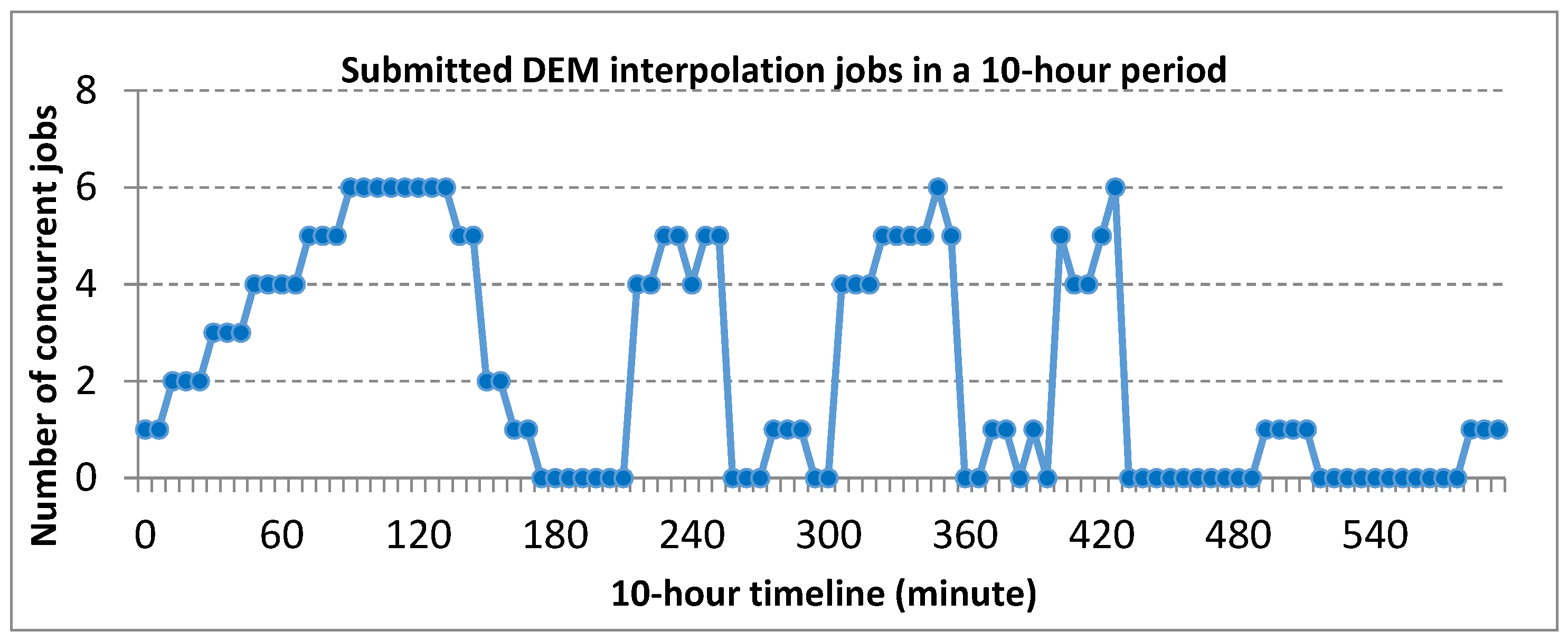
4.2.1. DEM Interpolation and Dynamic Workload Simulation

DEM interpolation, a typical data- and computational-intensive operation in geoprocessing, was used to demonstrate the efficiency of the auto-scaling framework for supporting geospatial data processing. Inverse Distance Weighting (IDW) was selected as the DEM interpolating algorithm, and a DEM interpolation MapReduce program was developed with JAVA programming language. The DEM data for the whole state of Kansas, USA, downloaded from the National Map Seamless Server (NMSS), was used as the test dataset (1 arc-sec, 30 m by 30 m spacing, ~900 Mb). To enable parallel interpolation with MapReduce, the DEM data were spatially decomposed into equal-sized tiles. The tiles were then reorganized into the Hadoop SequenceFile (https://wiki.apache.org/hadoop/SequenceFile) format and loaded to the CoveringHDFS for processing.

In order to simulate the dynamic geoprocessing workload, we submitted a different number of concurrent DEM interpolation requests (MapReduce jobs) to the cluster every six minutes over a 10-h period with each request processing a subset of the DEM dataset (~200 Mb). Each request can be considered as a workload for the computing cluster, and in total 100 workloads consisting of 224 DEM interpolation jobs were submitted. Figure 4 shows the patterns of the submitted processing workload during this period. The rationale for using this pattern design is that it represents typical workload dynamics of increasing (from 0 to 100 min), decreasing (130 to 180 min), on-off and periodical busting (200 to 420 min), and light or idle workload (420 to 600 min) patterns.

4.2.2. Hadoop Cluster Setup

Three Hadoop clusters in our private cloud environment were used for the sake of comparison: (1) an auto-scaling cluster based on the proposed framework; (2) a static cluster with seven slave nodes; (3) another static cluster with 14 slave nodes. The detailed configuration for the three clusters is shown in

Table 1. Three types of Hadoop clusters.

Cluster Type	Master	Slaves	HDFS
Auto-scaling cluster	One medium instance	Dynamic, start with three core-slaves with medium instances, can scale up 12 compute-slaves with small instances	CoveringHDFS, starting with 3 core-slaves
Seven-slave cluster	One medium instance	Static, 7 slaves with three medium instances and four small instances	Traditional HDFS with 7 slaves
Fourteen-slave cluster	One medium instance	Static, 14 slaves with three medium instances and 11 small instances	Traditional HDFS with 14 slaves

Medium instance: 2-core CPU, 2 GB RAM, 10 GB storage; and small instance: 1-core CPU, 1 GB RAM, 8 GB storage. For all clusters, each slave node was configured with two map slots and one reduce slot.

. All three clusters used one medium instance as the master node. The auto-scaling cluster started with three core-slaves, serving as the covering HDFS and capable of scaling up 12 compute-slaves during the peak workload. The two static clusters were used as baselines to compare with the auto-scaling cluster. In comparison to the workloads discussed previously, the static cluster with seven slaves served as a cluster with less capability, while the static cluster with 14 slaves acted as a full-powered cluster (best performance was archived using 14 slaves for the most intensive workload in our testing environment).

4.3. Result and Discussion

For the three clusters, the time spent on finishing each job was recorded, and the time consumed by each workload was derived by aggregating the individual job time. The result is shown in Figure 5.

4.3.1. Performance

Generally, the workload finish time for each cluster has a similar pattern as the workloads pattern (Figure 5). However, the seven-slave cluster responded more sensitively to the spike workloads, especially when the workloads were maintained at a high level over a relatively long time as illustrated at the 90 to 150-min period. Thus, when the workloads exceeded the capacity of the cluster, the processing requests were queued and could only be processed when previous jobs were finished. The queue became longer with the increase in workload, which in turn lengthened the time to finish. Therefore, the cluster with a fixed number of slaves had very limited capacity to handle the dynamic workload unless being provisioned for the peak workload.

For the auto-scaling cluster, the time consumed by each workload showed a similar pattern to that of the fourteen-slave full-powered cluster. As illustrated in the zoomed-in view of Figure 5, the auto-scaling cluster had sharper fluctuations than the fourteen-slave cluster for the first 1.5 h. These sharp jumps occurred during the scaling-up when the cluster was running with the under-powered mode. Once scaling up was finished, the cluster was in the full-power mode for current workload which explains the sharp drop in the workload finish time. This process is further illustrated in Figure 6A, where the changing size of the auto-scaling cluster driven by the dynamic workloads in the 10-h period is evident. The auto-scaling cluster effectively handled the increasing and burst workload patterns by increasing the computing power (compute-slaves) to ensure the jobs were finished within an acceptable time. Overall, the auto-scaling cluster shows similar performance to the full-powered cluster.

4.3.2. Resource Consumption

To evaluate resource consumption and the utilization rate of the auto-scaling cluster, the number of slaves (Figure 6A) and idle slaves (Figure 6B) of the three clusters were recorded during the 10-h period to monitor the slave status. Figure 6B shows the general pattern of idle slaves following the pattern of workloads but with an opposite direction. When the workload peaked, all three clusters have no idle slaves. When the workload ebbed, the fourteen-slave cluster had the largest number of idle slaves, while the auto-scaling cluster had the fewest idle slaves, and the seven-slave cluster is between these two extremes.

To better evaluate the performance and resource utilization of the auto-scaling cluster in a quantitative manner, the processing times of the 224 DEM interpolation jobs for each cluster were summed (Figure 7A). In addition, the Cluster Idle Slave Time (CIST) for each cluster was calculated (Figure 7B). CIST is defined as the sum of idle time for each slave of a cluster in a given time period. The auto-scaling cluster spent 18.59 h to complete all jobs, only 12 min longer than the 18.38 h of the fourteen-slave cluster (Figure 7A). Compared to the seven-slave cluster, the auto-scaling cluster spent 23 fewer hours (2.2X increase in performance) in completing all jobs. For the resource utilization, the auto-scaling cluster had the lowest idle time (16.2 h), 80% less than that of the idle time for the fourteen-slave cluster (78.2 h), saving 62 instance hours in the 10-h period (Figure 7B). If the cluster were to run for one month with repeated workload patterns, the auto-scaling cluster would save 4464 instance hours. This is equivalent to saving ~$232/month if this cluster were deployed on Amazon EC2 using the similar instance format (EC2’s t2.medium instance type pricing at $0.052/h not including the storage, network, and other costs [38]).

4.3.3. Data Locality

Within CoveringHDFS, core-slaves not only provide computing resources but also serve as the data storage and Input/Output (I/O) channels of the whole computing cluster. Processing tasks took place on core-slaves which could take advantage of data locality. For a physical cluster, more core-slaves provide more I/O capacity for the cluster and better make use of data locality while decreasing auto-scaling flexibility (since core-slaves cannot be terminated even they are idle to avoid data loss) and vice versa. However, in a cloud environment with virtualized storage and network resources, such an impact is more related to the cloud virtualization and storage mechanism. In our private cloud testing environment, the auto-scaling cluster has three core slaves while the other two fix-sized clusters use traditional HDFS. As indicated by the result (Figure 5), the CoveringHDFS does not cause an obvious performance degradation to the whole cluster as it showed similar performance as the fourteen-slave cluster with traditional HDFS.

From another aspect, this framework offers more control and flexibility to balance the performance and cost. In a performance-oriented application, one could always use a large number of core-slaves to ensure the performance. If cost is a more important factor, one could use a small number of core-slaves so that the cluster becomes light weight when the workload is low. In both cases, when the workload exceeds cluster capacity, more compute-slaves can always be added (assuming it would not exceed the cloud capacity) in minutes to bust the performance.

Generally, the fourteen-slave cluster maintained an excellent performance when the workload was high but wasted more computing resources (more idle slaves, Figure 7B) when the workload was low. The seven-slave cluster showed better resource utilization as compared to the fourteen-slave cluster but sacrificed performance (Figure 5) when the workload was high. By dynamically adjusting the cluster size based on the workload, the auto-scaling cluster showed overall the best resource utilization (the lowest idle time, Figure 7B) while delivering noticeably better performance (nearly equal to that of the fourteen-slave cluster, Figure 7). Acting like a car’s “automatic transmission”, this auto-scaling mechanism ensures that the right amount of power is delivered for the right workload, thus improving “energy efficiency”.

5. Conclusions

An auto-scaling framework is proposed to automatically scale cloud computing resources for Hadoop cluster based on the dynamic processing workload, with the aim of improving the efficiency and performance of big geospatial data processing. The most seminal components of this framework are the following: a predictive scaling-up algorithm considering the scale-up time proposed to accurately determine the number of slaves to be added by monitoring the white-box-based metrics; a CoveringHDFS mechanism to scale down the cluster promptly so as to avoid unnecessary resource consumption.

The feasibility and efficiency of the scaling framework are demonstrated using a prototype based on a Eucalyptus cloud. Experiments evaluated the auto-scaling cluster from the perspectives of performance and resource utilization by simulating typical workload patterns in a 10-h period using DEM interpolation as an example. Results show this auto-scaling framework is able to (1) significantly reduce the computing resource utilization (by 80% in our experiment) while delivering similar performance as a full-powered cluster by dynamically adjusting the cluster size based on the changing workload; and (2) effectively handle the spike processing workload by increasing the computing resources (compute-slaves) to ensure the processing is finished within an acceptable time.

Although promising results were observed, there are limitations in our current study. Future research is required to further evaluate and improve the framework as suggested below:

• The auto-scaling cluster was only allowed to scale up 12 slaves in our experiment. The auto-scaling capability could be better evaluated if we can scale up further with a larger cloud. In addition, we plan to further test the framework on different public cloud platforms, such as Amazon EC2.
• When implementing the framework in a public cloud, it is desirable to investigate how to integrate the cloud service cost model into the auto-scaling algorithm to further enhance the resource utilization. For example, the minimum billing cycle of Amazon EC2 is one hour; there is no need to terminate an idle slave if it is not at the end of a billing cycle.
• The Hadoop-related big data processing platforms such as Spark [39] are gaining increasing popularity. While the CoveringHDFS mechanism is able to work with those platforms as long as they use HDFS for data storage, the manner in which to adjust the MapReduce-based scaling algorithm for programming models warrants further investigation.

Nevertheless, the proposed auto-scaling framework offers a novel approach to efficiently allocating the right amount of computing resources to the dynamic geoprocessing requests in an automatic manner. Such a cloud-enabled, auto-scalable computing cluster offers a powerful tool to process big geoscience data with optimized performance and reduced resource consumption. While DEM interpolation is used as an example, the proposed framework can be extended to handle other geoprocessing applications that run on Hadoop, such as the climate data analytical services powered by Hadoop and cloud computing [7,11]. In addition, the predictive scaling algorithm sheds lights on automatically scaling cloud computing resources for other data processing platforms beyond Hadoop. Finally, we believe that the proposed approach offers a valuable reference in planning better performed spatial applications in a cyberinfrastructure environment to more cost-efficiently address data- and computational intensity challenges in geospatial domains [40,41].

References

1. Lee, J.G.; Kang, M. Geospatial big data: Challenges and opportunities. Big Data Res. 2015, 2, 74–81. [Google Scholar] [CrossRef]
2. Yang, C.; Wu, H.; Huang, Q.; Li, Z.; Li, J. Using spatial principles to optimize distributed computing for enabling the physical science discoveries. Proc. Natl. Acad. Sci. 2011, 108, 5498–5503. [Google Scholar] [CrossRef] [PubMed]
3. Wang, S. A cyberGIS framework for the synthesis of cyberinfrastructure, GIS, and spatial analysis. Ann. Assoc. Am. Geogr. 2010, 100, 535–557. [Google Scholar] [CrossRef]
4. Asimakopoulou, E. Advanced ICTs for Disaster Management and Threat Detection: Collaborative and Distributed Frameworks: Collaborative and Distributed Frameworks; IGI Global: Hershey, PA, USA, 2010. [Google Scholar]
5. Yang, C.; Goodchild, M.; Huang, Q.; Nebert, D.; Raskin, R.; Xu, Y.; Fay, D. Spatial cloud computing: How can the geospatial sciences use and help shape cloud computing? Int. J. Digit. Earth 2011, 4, 305–329. [Google Scholar] [CrossRef]
6. Karimi, H.A. Big Data: Techniques and Technologies in Geoinformatics; CRC Press: Boca Raton, FL, USA, 2014. [Google Scholar]
7. Schnase, J.L.; Duffy, D.Q.; Tamkin, G.S.; Nadeau, D.; Thompson, J.H.; Grieg, C.M.; Webster, W.P. MERRA analytic services: Meeting the big data challenges of climate science through cloud-enabled climate analytics-as-a-service. Comput. Environ. Urban Syst. 2014. [Google Scholar] [CrossRef]
8. Huang, Q.; Yang, C. Optimizing grid computing configuration and scheduling for geospatial analysis: An example with interpolating DEM. Comput. Geosci. 2011, 37, 165–176. [Google Scholar] [CrossRef]
9. Buck, J.B.; Watkins, N.; LeFevre, J.; Ioannidou, K.; Maltzahn, C.; Polyzotis, N.; Brandt, S. SciHadoop: Array-based query processing in Hadoop. In Proceedings of the 2011 International Conference for High Performance Computing, Networking, Storage and Analysis, Seattle, DC, USA, 12–18 November 2011.
10. Eldawy, A.; Mokbel, M.F. A demonstration of spatial Hadoop: An efficient MapReduce framework for spatial data. Proc. VLDB Endow. 2013, 6, 1230–1233. [Google Scholar] [CrossRef]
11. Li, Z.; Hu, F.; Schnase, J.L.; Duffy, D.Q.; Lee, T.; Bowen, M.K.; Yang, C. A spatiotemporal indexing approach for efficient processing of big array-based climate data with MapReduce. Int. J. Geogr. Inf. Sci. 2016, 1–19. [Google Scholar] [CrossRef]
12. Gao, S.; Li, L.; Li, W.; Janowicz, K.; Zhang, Y. Constructing gazetteers from volunteered big geo-data based on Hadoop. Comput. Environ. Urban Syst. 2014. [Google Scholar] [CrossRef]
13. Li, Z.; Yang, C.; Jin, B.; Yu, M.; Liu, K.; Sun, M.; Zhan, M. Enabling big geoscience data analytics with a cloud-based, MapReduce-enabled and service-oriented workflow framework. PLoS ONE 2015. [Google Scholar] [CrossRef] [PubMed]
14. Pierce, M.E.; Fox, G.C.; Ma, Y.; Wang, J. Cloud computing and spatial cyberinfrastructure. J. Comput. Sci. Indiana Univ. 2009. [Google Scholar] [CrossRef]
15. Yang, C.; Raskin, R. Introduction to distributed geographic information processing research. Int. J. Geogr. Inf. Sci. 2009, 23, 553–560. [Google Scholar] [CrossRef]
16. Xia, J.; Yang, C.; Liu, K.; Gui, Z.; Li, Z.; Huang, Q.; Li, R. Adopting cloud computing to optimize spatial web portals for better performance to support Digital Earth and other global geospatial initiatives. Int. J. Digit. Earth 2015, 8, 451–475. [Google Scholar] [CrossRef]
17. Tu, S.; Flanagin, M.; Wu, Y.; Abdelguerfi, M.; Normand, E.; Mahadevan, V.; Shaw, K. Design strategies to improve performance of GIS web services. In Proceedings of the International Conference on Information Technology: Coding and Computing, Las Vegas, NV, USA, 5–7 April 2004.
18. Schadt, E.E.; Linderman, M.D.; Sorenson, J.; Lee, L.; Nolan, G.P. Computational solutions to large-scale data management and analysis. Nat. Rev. Genet. 2010, 11, 647–657. [Google Scholar] [CrossRef] [PubMed]
19. Dean, J.; Ghemawat, S. MapReduce: Simplified data processing on large clusters. Commun. ACM 2008, 51, 107–113. [Google Scholar] [CrossRef]
20. Chen, M.; Mao, S.; Liu, Y. Big data: A survey. Mob. Netw. Appl. 2014, 19, 171–209. [Google Scholar] [CrossRef]
21. Lin, F.C.; Chung, L.K.; Wang, C.J.; Ku, W.Y.; Chou, T.Y. Storage and processing of massive remote sensing images using a novel cloud computing platform. GISci. Remote Sens. 2013, 50, 322–336. [Google Scholar]
22. Krishnan, S.; Baru, C.; Crosby, C. Evaluation of MapReduce for gridding LIDAR data. Cloud Comput. Technol. Sci. 2010. [Google Scholar] [CrossRef]
23. Aji, A.; Wang, F.; Vo, H.; Lee, R.; Liu, Q.; Zhang, X.; Saltz, J. Hadoop GIS: A high performance spatial data warehousing system over MapReduce. Proc. VLDB Endow. 2013, 6, 1009–1020. [Google Scholar] [CrossRef]
24. Leverich, J.; Kozyrakis, C. On the energy (in) efficiency of Hadoop clusters. ACM SIGOPS Oper. Syst. Rev. 2010, 44, 61–65. [Google Scholar] [CrossRef]
25. Kaushik, R.T.; Bhandarkar, M. GreenHDFS: Towards an energy-conserving storage-efficient, hybrid Hadoop compute cluster. In Proceedings of the USENIX Annual Technical Conference, Boston, MA, USA, 23–25 June 2010.
26. Maheshwari, N.; Nanduri, R.; Varma, V. Dynamic energy efficient data placement and cluster reconfiguration algorithm for MapReduce framework. Futur. Gener. Comput. Syst. 2012, 28, 119–127. [Google Scholar] [CrossRef]
27. Mell, P.; Grance, T. The NIST definition of cloud computing. Natl. Ins. Stand. Technol. 2009, 53, 1–7. [Google Scholar]
28. Getting Started with Hadoop with Amazon’s Elastic MapReduce. Available online: http://www.slideshare.net/DrSkippy27/amazon-elastic-map-reduce-getting-started-with-hadoop (accessed on 20 September 2016).
29. Baheti, V.K. Windows azure HDInsight: Where big data meets the cloud. IT Bus. Ind. Gov. 2014. [Google Scholar] [CrossRef]
30. Herodotou, H.; Dong, F.; Babu, S. No one (cluster) size fits all: automatic cluster sizing for data-intensive analytics. In Proceedings of the 2nd ACM Symposium on Cloud Computing, Cascais, Portugal, 26–28 October 2011.
31. Agrawal, D.; Das, S.; Abbadi, A. Big data and cloud computing: Current state and future opportunities. In Proceedings of the 14th International Conference on Extending Database Technology, Uppsala, Sweden, 21–25 March 2011.
32. Wang, Y.; Wang, S.; Zhou, D. Retrieving and Indexing Spatial Data in the Cloud Computing Environment; Springer: Berlin/Heidelberg, Germany, 2009. [Google Scholar]
33. Huang, Q.; Li, Z.; Liu, K.; Xia, J.; Jiang, Y.; Xu, C.; Yang, C. Handling intensities of data, computation, concurrent access, and spatiotemporal patterns. In Spatial Cloud Computing: A Practical Approach; Yang, C., Huang, Q., Li, Z., Xu, C., Liu, K., Eds.; CRC Press: Boca Raton, FL, USA, 2015; Volume 16, pp. 275–293. [Google Scholar]
34. Li, Z.; Yang, C.; Huang, Q.; Liu, K.; Sun, M.; Xia, J. Building model as a service for supporting geosciences. Comput. Environ. Urban Syst. 2014. [Google Scholar] [CrossRef]
35. Röme, T. Autoscaling Hadoop Clusters. Master’s Thesis, University of Tartu, Tartu, Estonia, 2010. [Google Scholar]
36. Gandhi, A.; Thota, S.; Dube, P.; Kochut, A.; Zhang, L. Autoscaling for Hadoop clusters. In Proceedings of the NSDI 2016, Santa Clara, CA, USA, 16–18 March 2016.
37. Shvachko, K.; Kuang, H.; Radia, S.; Chansler, R. The Hadoop distributed file system. IEEE Comput. Soc. 2010. [Google Scholar] [CrossRef]
38. Amazon EC2 Pricing. Available online: https://aws.amazon.com/ec2/pricing/ (accessed on 22 September 2016).
39. Zaharia, M.; Chowdhury, M.; Franklin, M.J.; Shenker, S.; Stoica, I. Spark: Cluster computing with working sets. HotCloud 2010, 10, 10. [Google Scholar]
40. Yang, C.; Raskin, R.; Goodchild, M.; Gahegan, M. Geospatial cyberinfrastructure: Past, present and future. Comput. Environ. Urban Syst. 2010, 34, 264–277. [Google Scholar] [CrossRef]
41. Wang, S.; Armstrong, M.P. A theoretical approach to the use of cyberinfrastructure in geographical analysis. Int. J. Geogr. Inf. Sci. 2009, 23, 169–193. [Google Scholar] [CrossRef]
Figure 1. Auto-scaling framework.
Ijgi 05 00173 g001
Figure 2. The structure of the cloud-based Hadoop cluster with CoveringHDFS.
Ijgi 05 00173 g002
Figure 3. An example status of the jth loop of Equation (2).
Ijgi 05 00173 g003
Figure 4. One hundred workloads submitted to the cluster in a 10-h period with a time spacing of six minutes. A total of 224 jobs were submitted (each dot representing a workload).
Ijgi 05 00173 g004
Figure 5. Time consumed by each workload (100 workloads in total) for the three clusters in the 10-h period. The small diagram on the top-right corner is the zoomed-in view for the first 1.5 h.
Ijgi 05 00173 g005
Figure 6. (A) The size change of the auto-scaling cluster in the 10-h period (the number of slaves monitored every 30 seconds). The seven-slave and 14-slave clusters are represented as two parallel lines; (B) Number of idle slaves in the 10-h period.
Ijgi 05 00173 g006
Figure 7. (A) Time consumed for finishing all workloads for each cluster. Time calculated by summing the 224 job finish times; (B) Cluster Idle Slave Time (CIST) for each cluster in the 10-h period.
Ijgi 05 00173 g007