Smartphone-Based Pedestrian’s Avoidance Behavior Recognition towards Opportunistic Road Anomaly Detection ^†

Abstract

Road anomalies, such as cracks, pits and puddles, have generally been identified by citizen reports made by e-mail or telephone; however, it is difficult for administrative entities to locate the anomaly for repair. An advanced smartphone-based solution that sends text and/or image reports with location information is not a long-lasting solution, because it depends on people’s active reporting. In this article, we show an opportunistic sensing-based system that uses a smartphone for road anomaly detection without any active user involvement. To detect road anomalies, we focus on pedestrians’ avoidance behaviors, which are characterized by changing azimuth patterns. Three typical avoidance behaviors are defined, and random forest is chosen as the classifier. Twenty-nine features are defined, in which features calculated by splitting a segment into the first half and the second half and considering the monotonicity of change were proven to be effective in recognition. Experiments were carried out under an ideal and controlled environment. Ten-fold cross-validation shows an average classification performance with an F-measure of 0.89 for six activities. The proposed recognition method was proven to be robust against the size of obstacles, and the dependency on the storing position of a smartphone can be handled by an appropriate classifier per storing position. Furthermore, an analysis implies that the classification of data from an “unknown” person can be improved by taking into account the compatibility of a classifier.

1. Introduction

Road anomalies, such as cracks, pits, puddles and fallen trees, are generally identified from citizen reports and are repaired by administrative entities. In most cases, the reports are made by telephone or e-mail, which makes it difficult for the administrative entities to identify the location of the anomaly. To address this issue, administrative entities and third parties are attempting to provide smartphone-based applications that accept text and/or image reports with location information [1,2]. Such human-centric sensing is often called participatory sensing [3]. Although the success of these applications depends on people actively reporting tasks, very few of the citizens who downloaded these applications have actually reported anomalies [1]. Therefore, we propose a method to detect road anomalies implicitly based on opportunistic sensing. Opportunistic sensing is another human-centric sensing paradigm, in which the data collection process is automated without any user involvement [4].

To detect road anomalies, we focus on avoidance behaviors. Recognizing avoidance behaviors and aggregating events with locations can help to generate automatic anomaly reports. Automatic road anomaly detection techniques for cars and bikes have already been proposed [5,6,7,8,9], but these cases deal with relatively large movements. In contrast, we consider that pedestrians’ avoidance behaviors are too slight to make the adaptation of existing methods acceptable. The contributions of this article are as follows:

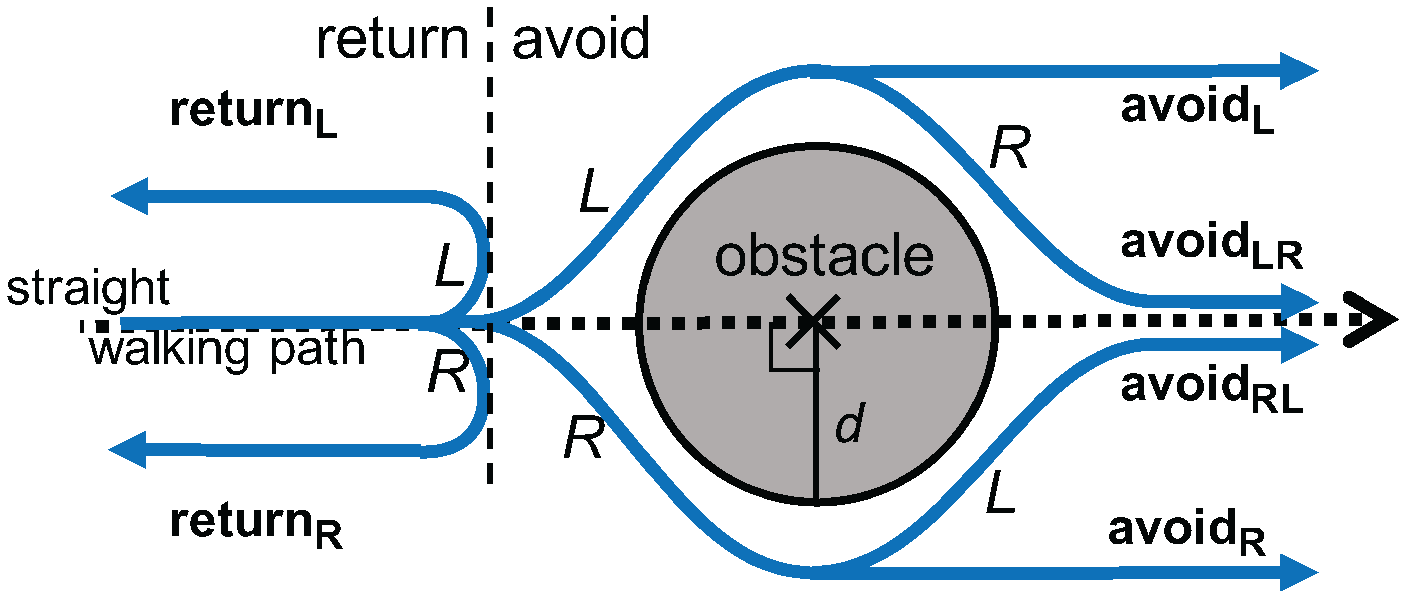
• A smartphone-based road anomaly detection system is presented, in which obstacle avoidance behaviors are categorized into three classes. The three classes include: (1) returning to the same line in the vicinity of avoiding an obstacle; (2) going straight after avoiding an obstacle; and (3) reversing his/her course; which may indicate the impact of the obstacle on pedestrians. The three classes may indicate the severity of obstacles, which would be helpful for an administrative entity to plan a repair schedule.
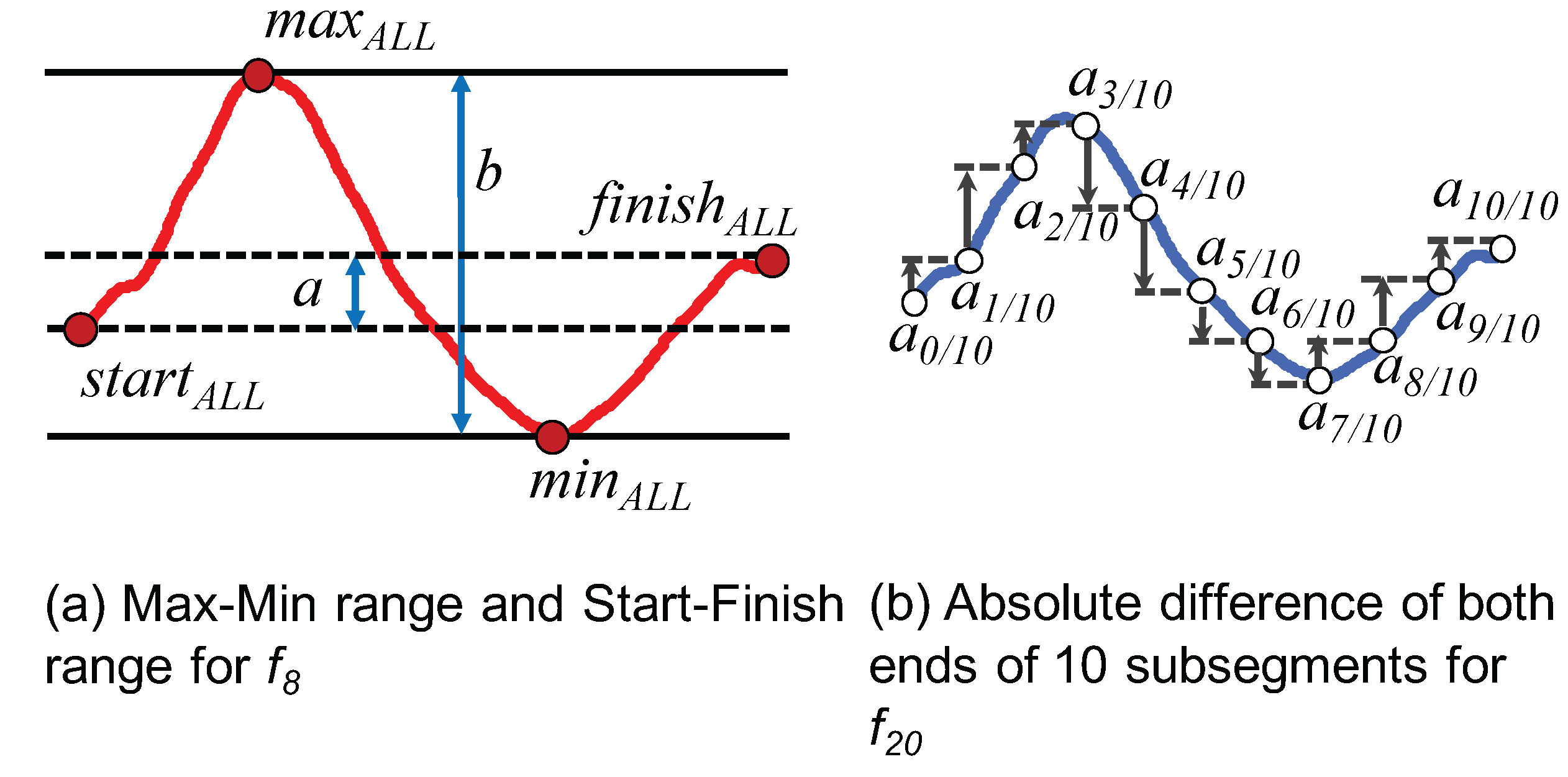
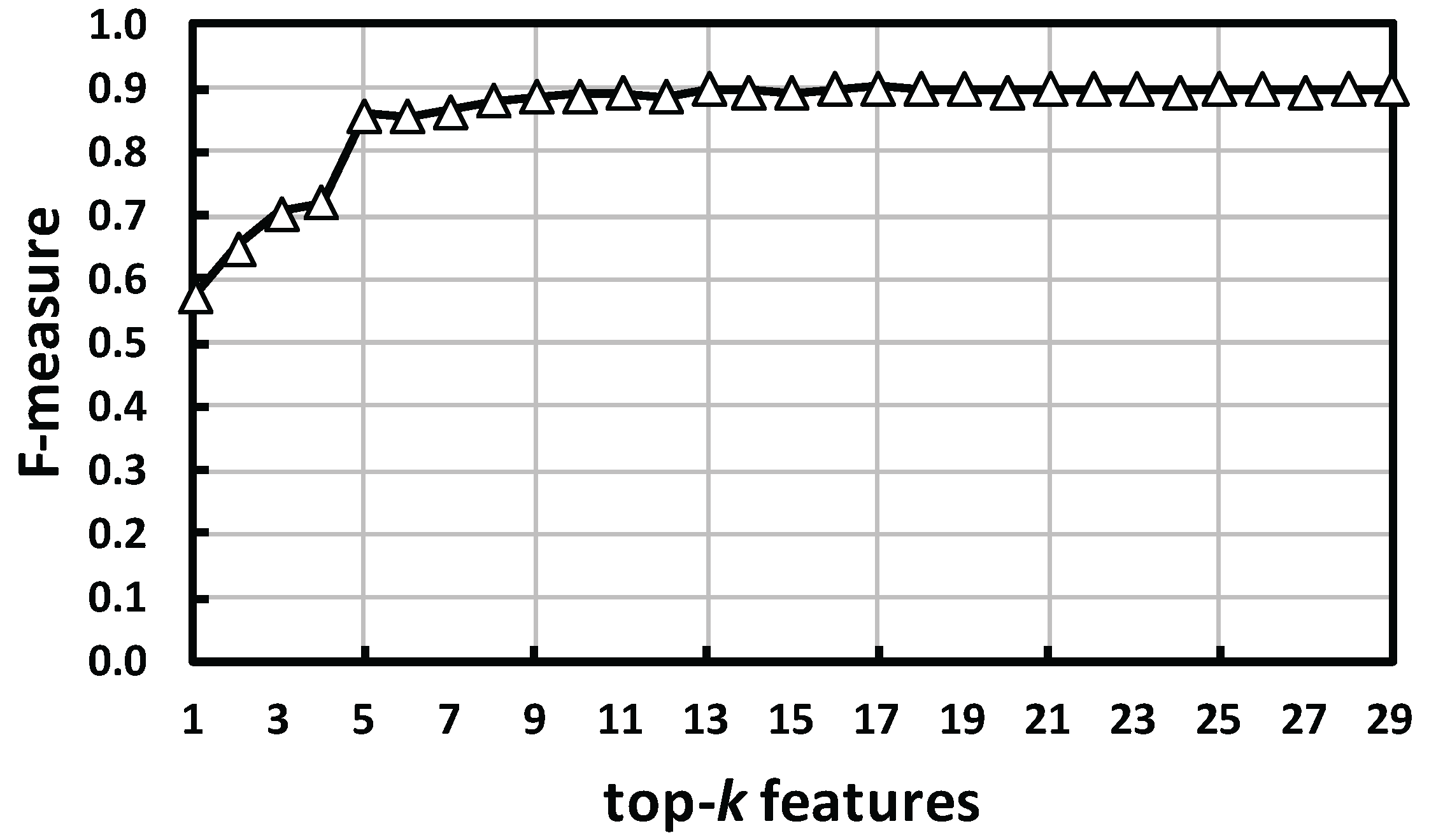
• Twenty nine classification features are defined based on the characteristics of the azimuth change of each class. The relevance of the features is evaluated.
• We extensively analyze the effects of various factors on the recognition performance. This includes the individuals who provide data for training classifiers and the position of sensors (i.e., smartphones) on their bodies, as well as the size of target obstacles.

An initial decision on the position and the class of an obstacle is made on the smartphone side against a stream of sensor data, while the collected information from a number of pedestrians is utilized to make the final decision. Low-power operation and server-side processing are beyond the scope of this article. Furthermore, we do not deal with a method of distinguishing a normal behavior, e.g., walking along a curved road, from avoidance behavior. Instead, we focus on classifying a data segment of avoidance behavior into one of six (three classes × right and left turns) classes.

The remainder of this article is organized as follows. In Section 2, related work is presented. Section 3 shows the system overview, followed by offline experiments in Section 4. Finally, Section 5 concludes the article. Note that, in [10], we proposed the basic idea of smartphone-based road anomaly detection. This article has extensions in the following points: a section of related work is added in order to clarify the uniqueness of the work (Section 2); the overall system ideas are presented, including not only the local processing on the smartphone, but also the server side processing to filter out erroneous detection from the smartphone side (Section 3.1); the detail of avoidance behavior recognition (on the smartphone) is described, including how the raw azimuth data stream is processed into the final avoidance event and detail definition of features (Section 3.3); experiments were carried out with different conditions, i.e., a type of behavior “straight” was excluded, because we considered it could be done in the preprocessing stage; and extensive analyses about person dependency (Section 4.4), sensor-storing position dependency (Section 4.5) and robustness to unknown obstacle size (Section 4.6) were undertaken.

2. Related Work

Motorcycles and other vehicles are often used as a method of automatic road anomaly detection and unsafe behavior detection [6,7,8,9,11,12,13,14]. Thepvilojanapong et al. [14] and Kamimura et al. [12] proposed a method using a smartphone-mounted accelerometer and gyroscope to detect driving activities, such as turning left or right, going forward or bicycles and motorcycles going past nearby cars. Iwasaki et al. [15] proposed a method to recognize road characteristics, such as an intersection with poor visibility and a congested road based on the bicycle riding behavior. Additionally, a special sensor unit that measures rudder angle and velocity was developed for bicycle riders to detect hazardous locations [8]. The vertical displacements of vehicles passing over bumps and potholes are often subject to monitoring in the case of cars [5,7,9,11,13]. In contrast, Chen et al. recognized driving factors that cause horizontal displacements, such as a lane change, S-shaped curved road, turning or L-shaped curved road [6]. In the above-mentioned work, all but [8] utilized a smartphone-mounted accelerometer, gyroscope and/or magnetometer. This shows the possibilities of smartphones as easy-to-deploy sensors in combination with a positioning technique, e.g., GPS. Furthermore, the aggregation of data followed by proper analysis can create new types of information content for comfortable and safe transport systems. Our work shares its motivations with the above studies. However, we focus on road anomalies from the pedestrian’s point of view. In addition, although the above-mentioned work on horizontal displacement [6,12,14,15] might find similar trajectories of moving objects, bicycles and cars have larger and faster movements than pedestrians, and so, applying the existing methods to our domain would be difficult.

For pedestrian-based road condition monitoring, Jain et al. proposed a shoe-based ground gradient sensing technique [16]. A sensing unit composed of a magnetometer, accelerometer and gyroscope is mounted on shoes, which collect data that detect the transitions between sidewalks and streets through the recognition of dedicated slopes. The primary motivation of those studies was to use the data to alert texting pedestrians who are about to step into the street. The slope sensing technique can also detect the vertical condition of sidewalks, e.g., bumps. Additionally, the shoes can detect turns and moving direction. These capabilities suggest that augmented shoes can be combined with our system as a sensor to detect horizontal behavior changes.

3. Avoidance Behavior Recognition

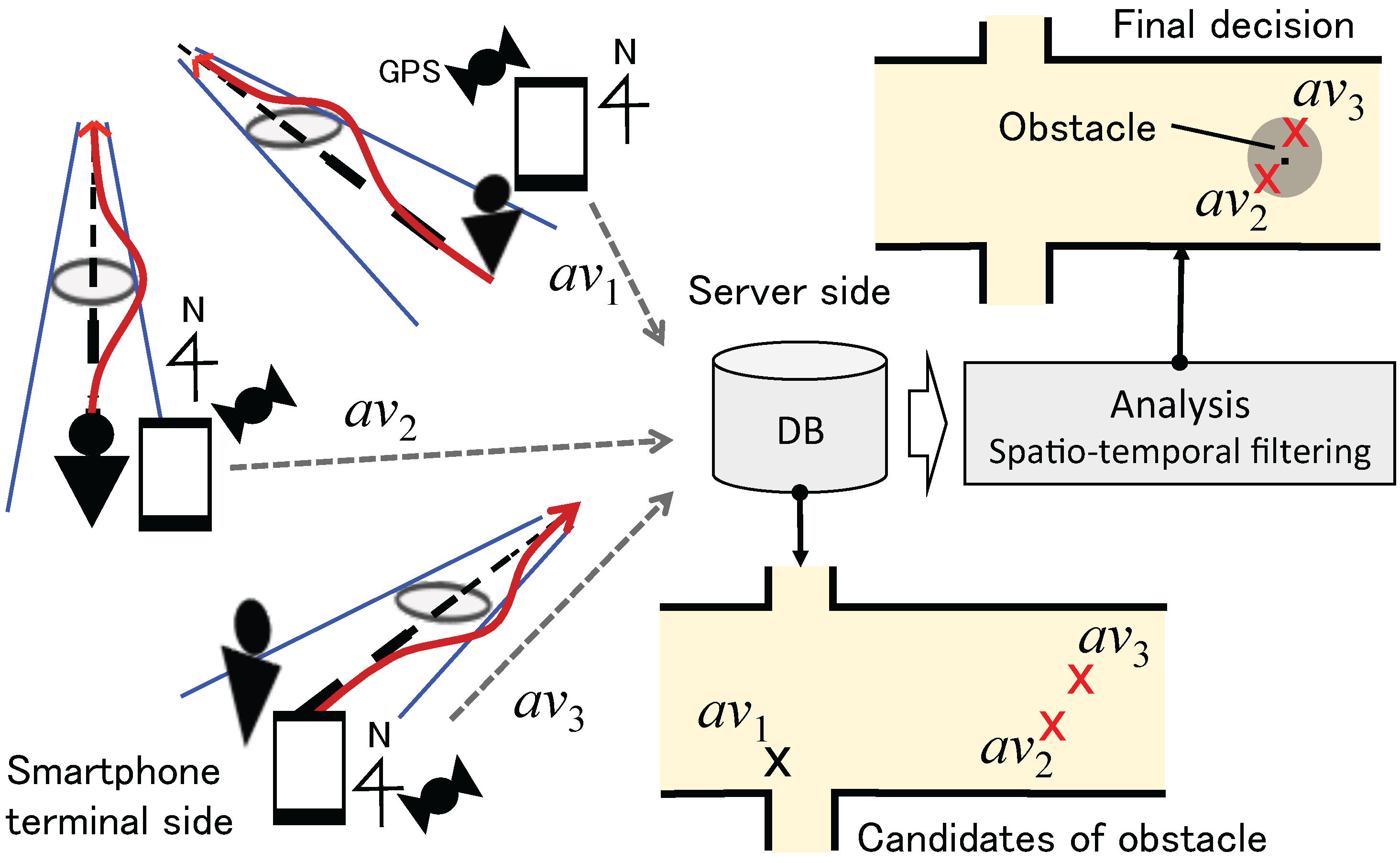
3.1. System Overview

Figure 1 illustrates the concept of the proposed system. The proposed system is designed to identify a road anomaly in an automatic manner, which consists of an avoidance behavior recognition function with location measurement on the smartphone side and aggregation and filtering functions on the server side. An avoidance behavior is recognized by measuring azimuth changes of the walking direction by a smartphone-mounted accelerometer and magnetometer. In the Android API, these two sensors are internally utilized to obtain azimuth data. The position where the avoidance event occurs is measured by a positioning technique, such as GPS. The information is sent to a database on the server side. In Figure 1, $a{v}_1$, $a{v}_2$ and $a{v}_3$ indicate the candidates of avoidance events. Note that power consumption is a central issue for the success of opportunistic sensing from the user’s point of view. To minimize the communication with a server, the processing for the avoidance event detection is carried out on the terminal side, and only events of avoidance behavior are sent to the server. Additionally, we assume the GPS receiver is activated only when an avoidance event is detected (the positional gap between the time of event detection and that of GPS-ready is also considered).

The aggregated information may contain erroneous events that are falsely recognized as avoidance behaviors, such as one person passing another person and looking behind with the smartphone terminal in his/her hand, as well as the effect of positioning error. Therefore, spatio-temporal filtering should be applied to extract only “static obstacles” on the road (e.g., [17]). In Figure 1, $a{v}_1$ is such a false detection, and the system finally identifies a road anomaly near the position of $a{v}_2$ and $a{v}_3$. Calculating the center of the positions of avoidance behavior events is a simple solution. Additionally, a geographical information system (GIS) for map-matching the position of an event on a road can be applied. A GIS can also be utilized to eliminate an event falsely classified as avoidance, which is actually normal behavior, by reflecting the semantics of the road, i.e., identifying that a curve exists at position (x, y). This article focuses on the avoidance recognition functionality on the smartphone side. Low-power positioning and server-side processing are beyond the focus of this article.

3.2. Avoidance Behavior Modeling

We focus on detecting anomalies on the road surface, such as pits, cracks, puddles, fallen trees and landslides. These anomalies make pedestrians change their walking paths as a natural defensive behavior [18]. The avoidance behavior during walking is modeled by the combination of three elements: (1) avoiding direction (left or right); (2) going through an obstacle (avoid) or going back (return); and (3) a direction change after avoiding an obstacle. In total, six types of avoidance behaviors are defined, as shown in Figure 2: $avoi{d}_{LR}$, $avoi{d}_L$, $avoi{d}_{RL}$, $avoi{d}_R$, $retur{n}_L$ and “$retur{n}_R$”. Here, the postfix “LR” indicates, for example, that the pedestrian changes direction to the left followed by a change to the right, whereas the postfix “L” alone does not have the second change after the first change to the left. The horizontal dotted line in Figure 2 indicates the pedestrian’s straight walking path. Furthermore, d represents the size of an avoidance behavior, which is primarily determined by the physical size of an obstacle, i.e., the avoidance behavior size equals the obstacle size. The perceived size may also affect the behavior or, in other words, the severity of the anomaly. We collectively call d “obstacle size” or “size of obstacle”. The typical waveforms of raw azimuth signals are shown in Figure 3.

3.3. Avoidance Behavior Recognition

As shown in Figure 4, the recognition system takes a segment of the azimuth data as input and classifies the segment into one of six behaviors. The recognition task should be performed on streaming sensor data. Sliding variance can be calculated on streaming data to emphasize the start and the finish of the change of walking direction. However, a change of walking direction also occurs when a pedestrian turns a corner or walks along a curved road, which are normal behaviors and should not be detected as obstacle avoidance. Therefore, special care is required to distinguish these situations from one another. Automatic segmentation is beyond the focus of this article, and we utilize manually-segmented data to focus on recognizing the six behaviors.

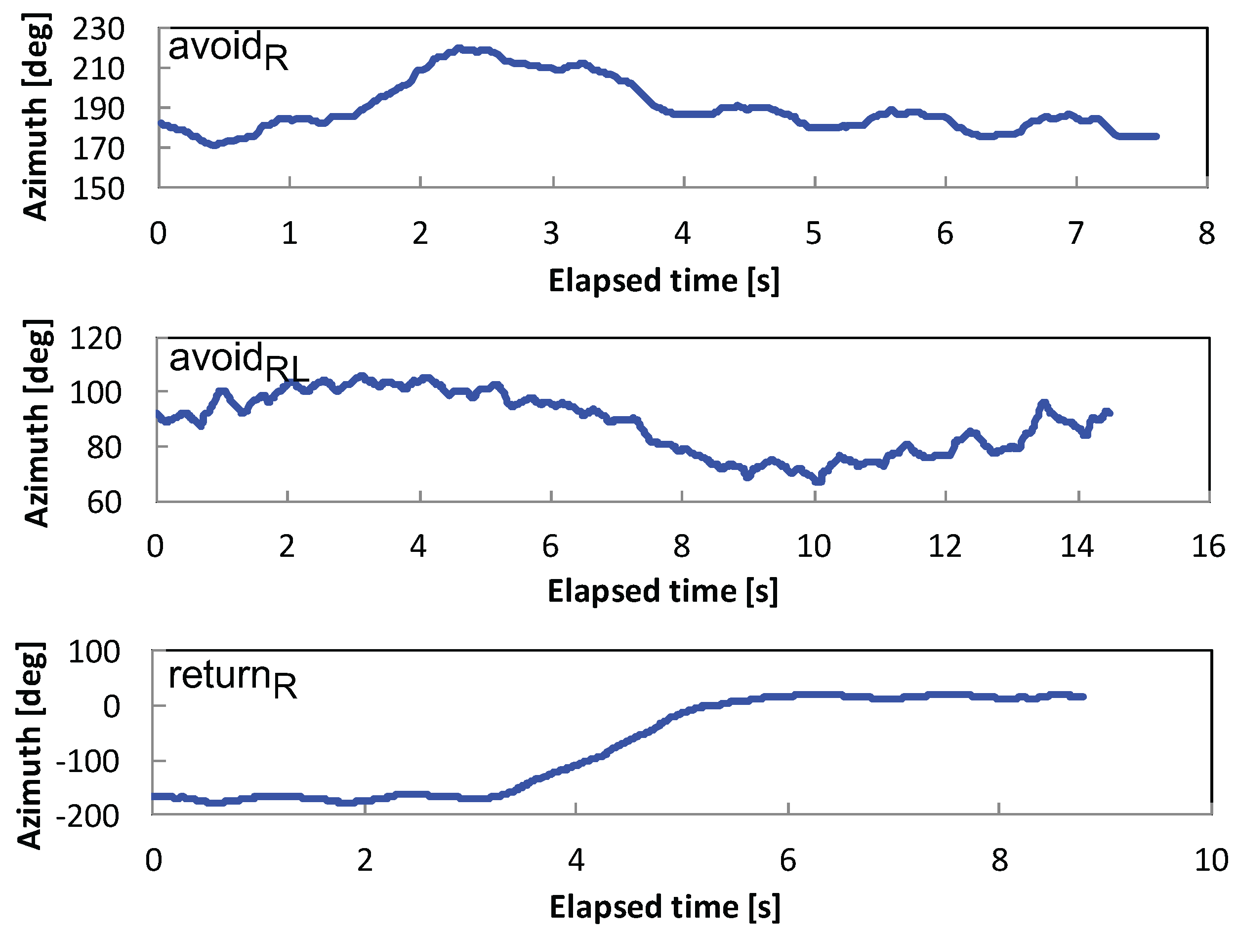
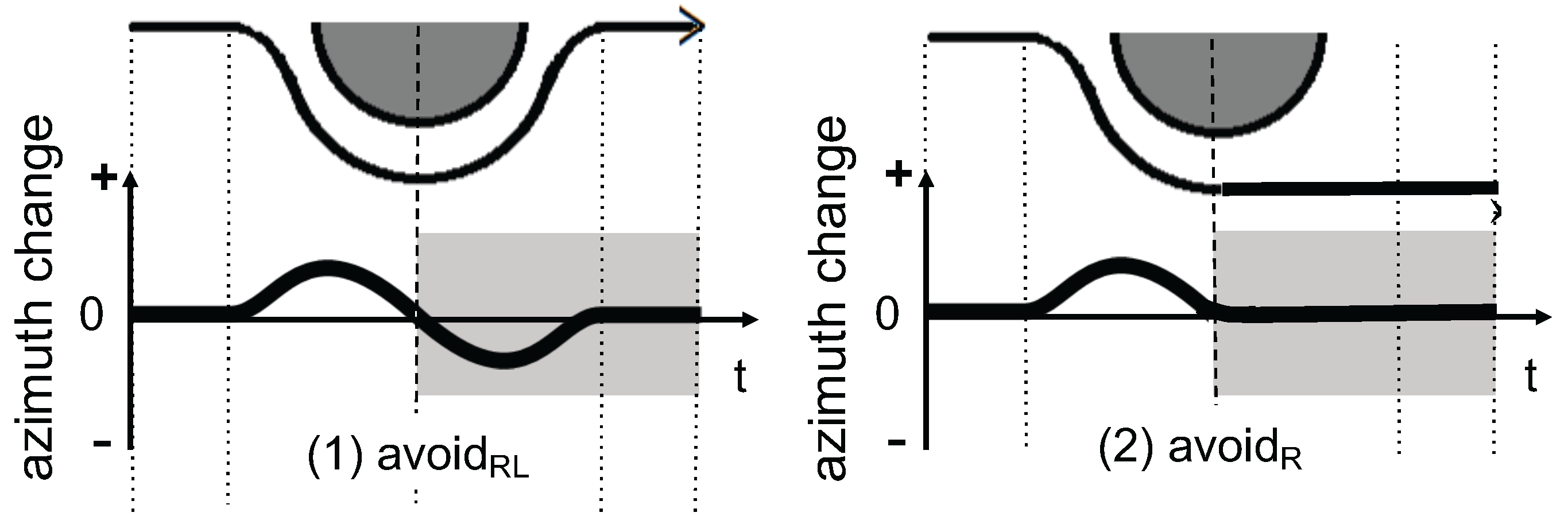
3.3.1. Waveform Shaping

The waveform shaping process works as a preprocess and is composed of azimuth change detection and smoothing. We obtain the azimuth value from an Android API. The value, which is calculated from accelerometer and magnetometer data, ranges from $0^{\circ }$ to ${359}^{\circ }$. Therefore, a non-contiguous change appears when the walking direction crosses the north, i.e., $0^{\circ }$, as observed in B’ of Figure 4. In this case, a person is supposed to change the direction from near west-northwest (P = $335.2^{\circ }$) to near east-northeast (Q = $21.4^{\circ }$). Furthermore, the value is normalized by converting it from the first value into a relative value. Then, the azimuth change in a segment is calculated by Algorithm 1, in which Lines 7 to 9 handle a non-contiguous change. The transformed signal is shown in C of Figure 4.

Algorithm 1 Calculate Azimuth Change Relative to the First Value in a Segment.

1: procedure AzimuthChange($a_{raw}$)     ▹$a_{raw}$ represents an array of a segment.  2:       $th\leftarrow 200$       ▹ A threshold value to judge if a non-contiguous change appears  3:       $segnum\leftarrow a_{raw}.length$  4:       $a_{change,0}\leftarrow 0$  5:       for $i\leftarrow 1,segnum-1$ do  6:            $\delta \leftarrow a_{raw,i}-a_{raw,i-1}$  7:            if $\left|\delta \right|>th$ then  8:                 $\delta \leftarrow \delta -sgn\left(\delta \right)\times 360$   ▹$sgn$(x) returns −1 if x < 0, 1 if x > 0, and 0 if x = 0.  9:            end if 10:           $a_{change,i}\leftarrow a_{change,i-1}+\delta$ 11:       end for 12:       return $a_{change}$    ▹ Returns an array of azimuth change relative to the initial value 13: end procedure

In addition, to remove the effect of body motion, i.e., smoothing, a moving average is applied as a low-pass filter, as shown in D of Figure 4. The window size for the moving averages is 1/6 of the segment of azimuth data, as determined in a preliminary experiment.

3.3.2. Behavior Classification

Behavior classification, which consists of feature calculation and supervised classification, is performed after waveform shaping. In total, we specified 29 features, which are summarized in

Table 1. Features, listed in order of contribution from upper left to lower right.

$f_1$	$mi{n}_{SH}$	$f_{16}$	$ma{x}_{FH}$
$f_2$	$ma{x}_{SH}$	$f_{17}$	$sumofsquare{s}_{SH}$
$f_3$	$mea{n}_{SH}$	$f_{18}$	$varianc{e}_{ALL}$
$f_4$	$su{m}_{SH}$	$f_{19}$	$standarddeviatio{n}_{ALL}$
$f_5$	$mea{n}_{FH}$	$f_{20}$	sum of absolute difference of
$f_6$	$mea{n}_{ALL}$		both ends of 10 subsegments
$f_7$	$media{n}_{ALL}$	$f_{21}$	$su{m}_{FH}$
$f_8$	$ratioofrang{e}_{ALL}to\Delta SF$	$f_{22}$	$IQ{R}_{ALL}$
$f_9$	$su{m}_{ALL}$	$f_{23}$	$3rdquartil{e}_{ALL}$
$f_{10}$	$rang{e}_{ALL}$	$f_{24}$	$1stquartil{e}_{ALL}$
$f_{11}$	$mi{n}_{ALL}$	$f_{25}$	$RM{S}_{ALL}$
$f_{12}$	$absolutemi{n}_{ALL}$	$f_{26}$	$sumofsquare{s}_{ALL}$
$f_{13}$	$ma{x}_{ALL}$	$f_{27}$	$varianc{e}_{FH}$
$f_{14}$	$absolutema{x}_{ALL}$	$f_{28}$	$sumofsquare{s}_{FH}$
$f_{15}$	$mi{n}_{FH}$	$f_{29}$	$varianc{e}_{SH}$

ALL: an entire segment; FH and SH: first half and second half of a segment; IQR: inter-quartile range; RMS: root mean square; ΔSF: absolute difference between values at the start and the finish.

. These features mainly contain basic statistics, such as mean, maximum, minimum, range, first and third quartiles, inter-quartile range (IQR), variance, standard deviation, summation, summation of squares, root mean square (RMS) and absolute values. In lining up features, we paid special attention to the fact that the trajectories of $avoi{d}_{RL}$ and $avoi{d}_R$ are clearly distinguished from each other after passing an obstacle (Figure 5), so we split a segment into two parts at the center of the segment. Features calculated from the first half segment and the second half segment have subscripts FH and SH, respectively. In contrast, features from an entire segment have the subscript ALL. Note that Table 1 is listed in order of contribution to the classification. Not all of the corresponding effects of features can be significant or could even have a negative impact, which is discussed in Section 4.3.

To calculate the eighth feature, ($f_8$) is introduced to represent the monotonicity of the azimuth change in a segment. As shown in Figure 6a and expressed by Equation (1), the feature gets larger as the maximum ($ma{x}_{ALL}$) and the minimum ($mi{n}_{ALL}$) values approach both ends ($star{t}_{ALL}$ and $finis{h}_{ALL}$). We consider that “$retur{n}_R$” has the largest value of the three behaviors because the azimuth change of “$retur{n}_R$” is ideally a monotonic increase or decrease (see Figure 5).

$$f_8=|\frac{ma{x}_{ALL}-mi{n}_{ALL}}{star{t}_{ALL}-finis{h}_{ALL}}|$$

(1)

For the 20th feature ($f_{20}$), a segment is equally divided into 10 subsegments, and the absolute difference between both ends of each subsegment is summed up to 10 subsegments. The notation is illustrated in Figure 6b, as well as expressed by Equation (2). The rationale for introducing this feature is that a behavior with a large azimuth change tends to have a large absolute difference. As shown in Figure 5, $avoi{d}_R$ has a smaller value than $avoi{d}_{RL}$ due to a lack of azimuth change in the second half of the segment. Meanwhile, $retur{n}_R$ should have the largest change because the walking direction changes to the opposite side.

$$f_{20}=\sum _{i=0}^9|a_{(i+1)/10}-a_{i/10}|$$

(2)

Regarding the recognition (classification) functionality, handmade rule-based approaches [6,12], a statistical machine learning approach (J48decision tree) [8] and a probabilistic approach (hidden Markov model (HMM)) [14] were utilized in the literature of horizontal displacement recognition. A handmade rule-based approach can be considered as a form of decision tree in that “if-then” rules are set using the expert knowledge. Therefore, the decision-making process is more interpretive than what the J48 decision tree provides; however, the approach requires the careful design of the rule, and thus, the case with a small number of recognition classes seems to be suitable, e.g., three for [6] and two for [12]. The avoidance behavior recognition problem can be regarded as a time series pattern recognition, in which HMM is one of the following: popular approach speech [19], hand-written character [20] and gesture recognition [21]. However, the HMM-based system is considered to require a sizable amount of training to data to perform well [22,23]. Based on these considerations, we utilized a supervised learning classifier. The comparison among various types of classifiers is presented in Section 4.2.

4. Offline Experiment

An offline experiment was carried out on various aspects, such as contributing features and the difference in individuals, the storing positions and the sizes of obstacles, in addition to the basic classification performance.

4.1. Dataset

Data collection was performed as summarized in

Table 2. Condition of data collection.

Types of avoidance	$avoi{d}_{RL}$, $avoi{d}_R$, $retur{n}_R$
Size of obstacles (d)	0.2, 0.5, 0.7, 1.0, 1.5 m
Storing positions	hand (texting), trousers front pocket, trousers back pocket, chest pocket
Subjects	7 males and 2 females in their 20s
Number of trials	6 times per condition
Terminal	Samsung, Galaxy Nexus
Android version	Android 4.2.1
Sensor type	Sensor.TYPE_ORIENTATION
Sampling rate	10 Hz

, and Figure 7 shows a scene of data collection. A “cross” mark was placed on the ground as an obstacle. Subjects were asked to walk on a straight path while avoiding obstacles with directed types of avoidance behaviors. They started walking about seven meters behind the center of the obstacle. The timing of the start and the finish in each avoidance behavior was based on their decisions, although they were asked to walk past a mark that represented the edge of an obstacle. The segmentation was done by hand.

In addition to the original data, we synthesized $avoi{d}_{LR}$, $avoi{d}_L$ and $retur{n}_L$ based on the findings that avoidance behaviors have left-right symmetry [18]. As shown by Equation (3), the synthesis is realized by inverting the sign of each sample. Here, $a_{L,k}$ and $a_{R,k}$ indicate the k-th sample in the collected data and in the synthesized data, respectively. Finally, the profile of the collected and synthesized dataset is summarized in

Table 3. Profile of the dataset.

Type	Segments	Person	Segments	Size	Segments
$avoi{d}_{RL}$	865	A	540	0.2	844
$avoi{d}_R$	866	B	262	0.5	486
$avoi{d}_{LR}$	865	C	508	0.7	838
$avoi{d}_L$	866	D	528	1.0	480
$retur{n}_R$	215	E	288	1.5	814
$retur{n}_L$	215	F	336	Stored	Segments
		G	358	hand	952
		H	538	trousers front pocket	966
		I	534	trousers back pocket	968
				chest pocket	1006

. Note that data with obstacle sizes 0.5 and 1.0 m were only used in Section 4.6 to evaluate the robustness of the classifier against the unknown size of obstacles.

$$a_{L,k}=-a_{R,k}$$

(3)

Note that the azimuth measurement relies on the magnetometer that may be affected by architectural construction, including metal, high-voltage current and magnetism. The data collection was carried out in an environment where no building and machinery exist around the subjects, in which we did not observe any unstable reading from the sensor. However, to observe if any disturbance in sensor reading exists, we empirically walked near air conditioner’s outdoor units, vehicles, vending machines, exterior wall of buildings, etc., and visually checked a graph of the data stream. As a result, we found disturbance in very limited cases of passing by an electric vehicle and passing through a narrow passage surrounded by a reinforced concrete wall. In both cases, the data appear to be randomly and rapidly changing. Therefore, we consider that such a situation is distinguishable to avoid misrecognition of avoidance behavior; however, further study is required to recognize an avoidance behavior that occurs in such a situation.

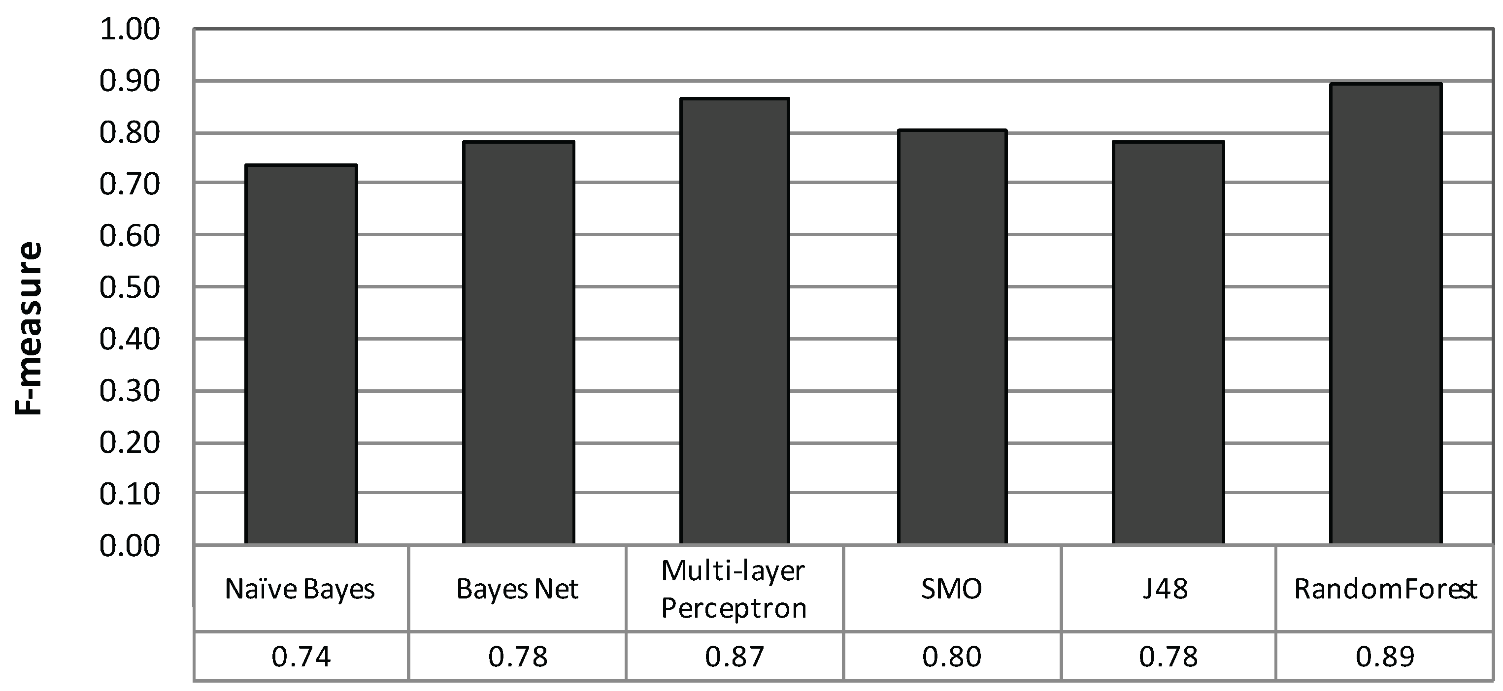
4.2. Basic Classification Performance

4.2.1. Method

First of all, various types of classification methods, i.e., classifiers, are compared by applying 10-fold cross-validation (CV) to fix one classifier for later evaluation. Here, naive Bayes (a baseline approach), Bayesian network (a graphical model approach), multi-layer perceptron (MLP, an artificial neural network approach), sequential minimal optimization (SMO, a support vector machine approach), decision tree (J48) and random forest (an ensemble learning approach) were used.

Table 4. Classifier parameters in Weka.

Classifier	Parameter
Naive Bayes	N/A
Bayesian network	-Q K2 “-P 1 -S BAYES” -E SimpleEstimator “-A 0.5”
MLP	-L 0.3 -M 0.2 -N 500 -V 0 -E 20 -H a
SMO	-C 1.0 -P 1.0E-12 -K “PolyKernel -E 1.0 -C 250007”
J48	-C 0.25 -M 2
Random forest	-I 100 -K 0

summaries the parameters for each classifier used in a machine learning toolkit Weka ver. 7.3.13 [24], in which default values were utilized. The parameter symbols can be referred to as the reference manual of Weka.

4.2.2. Result and Analysis

Figure 8 shows the F-measure of each classifier, in which random forest performed the best followed by MLP. Another advantage of random forest is the small number of tuning parameters. In the Weka implementation, the number of major parameters is two, while that of MLP is five. Therefore, we consider that random forest is easy for tuning. Hereinafter, random forest with 100 trees is utilized.

Table 5. Confusion matrix of 10-fold cross-validation (CV) using random forest.

Label\Recognition	(1)	(2)	(3)	(4)	(5)	(6)
(1) $avoi{d}_{RL}$	182	19	7	7	0	0
(2) $avoi{d}_R$	25	179	6	6	0	0
(3) $avoi{d}_{LR}$	7	6	183	19	0	0
(4) $avoi{d}_L$	7	6	24	179	0	0
(5) $retur{n}_R$	0	0	0	0	215	0
(6) $retur{n}_L$	0	0	0	0	0	215

shows the confusion matrix, in which the row indicates the labeled class and the column is the recognition result.

Table 6. Recall, precision and F-measure using random forest.

Class	Recall	Precision	F-Measure
$avoi{d}_{RL}$	0.85	0.83	0.84
$avoi{d}_R$	0.83	0.85	0.84
$avoi{d}_{LR}$	0.85	0.83	0.84
$avoi{d}_L$	0.83	0.85	0.84
$retur{n}_R$	1.00	1.00	1.00
$retur{n}_L$	1.00	1.00	1.00
Average	0.89	0.89	0.89

summarizes the results of recall, precision and F-measure. Note that we normalized the recognition results by the smallest number of segments throughout this article because the number of data varies by class, as shown in Table 3. The result shows an average classification performance with an F-measure of 0.89 and a range from 0.84 to 1.00.

Classes $avoi{d}_{RL}$ and $avoi{d}_{LR}$ were misclassified into $avoi{d}_R$ and $avoi{d}_L$, respectively. We consider that this occurred because the second half of the segment of these classes is flat, which made it difficult to distinguish the classes from each other. In contrast, $retur{n}_R$ and $retur{n}_L$ were perfectly classified. We assumed that the start and the end of the walking direction of $avoid$ are identical, whereas the start and the end of $return$ are different, i.e., on the opposite side. We consider that the features of $return$ had large differences from those of $avoid$.

The recognition of road anomaly class is useful for a road administration office; however, to prioritize their repairing tasks, the size of the road anomaly should be recognized, since a large avoidance behavior indicates the significance of the anomaly. Currently, we have a dataset with five obstacle sizes. Defining new classes for each size is not practical. Therefore, we will build a regression model based on some features and the obstacle size, which will be applied after classifying datasets into the six avoidance behavior classes.

4.3. Feature Relevance

4.3.1. Method

To understand effective features for avoidance behavior recognition, the relevance of features was evaluated based on information theory. Information gain is commonly used in feature selection, where the gain of information provided by a particular feature is calculated by subtracting a conditional entropy with that feature from the entropy under a random guess [25]. We used InfoGainAttributeEval and Ranker in Weka [24] as implementations for evaluating information gain and generating ranking, respectively.

As described in Section 3.3.2, Table 1 is already listed in order of contribution (relevance) with the above implementations. To observe the change of classification performance against the number of features, a 10-fold cross-validation was carried out against a dataset with the top-k features, and F-measures were calculated. Here, k varies from one (best) to 29 (all).

4.3.2. Result and Analysis

As shown in Figure 9, the F-measure for the top five features rapidly increases. From the top six to 20 features, the F-measure gradually increases by very slight up-and-down movements. Finally, the increase almost levels off for more than 20 features. As described in Section 3.3.2, we split a segment into two parts: first half (FH) and second half (SH) (see Figure 5). By looking at Table 1, the top-four contributing features are derived from SH. This indicates that the decision to calculate features by dividing them into FH and SH proved to be correct. Note that the division of the two parts is based on the number of samples in a segment under the assumption that people walk at a constant velocity; however, in practice, the speed might change in the vicinity of an obstacle. This makes the two divided parts not as clear as those shown in Figure 5. Detecting such a changing point would emphasize the difference of activities more clearly and improve the performance.

Furthermore, the “ratio of ${\text{range}}_{ALL}$ to ΔSF” ($f_8$), which was added to get the the monotonicity of the change, appeared as the eighth in the ranking. In the two-thirds of the ranking, features that eliminate negative values are found ($f_{12}$, $f_{14}$, $f_{17}$, $f_{25}$, $f_{26}$ and $f_{28}$). This implies that the component of direction is more important than the magnitude of movement. As opposed to the expectation on the accumulated azimuth change described in Section 3.3.2, “sum of the absolute difference of both ends of 10 subsegments” appears in the 20th ranking ($f_{20}$). We consider that $f_{20}$ contributes to discriminate $return$ from $avoid$ because of the large change in the direction. However, the difference of the accumulated change between $avoi{d}_R$ and $avoi{d}_L$ is not so large as other features and less contributive. Furthermore, since $f_{20}$ represents the amount of change, it is difficult to discriminate $avoi{d}_{RL}$ from $avoi{d}_{LR}$, which are symmetric about the horizontal axis.

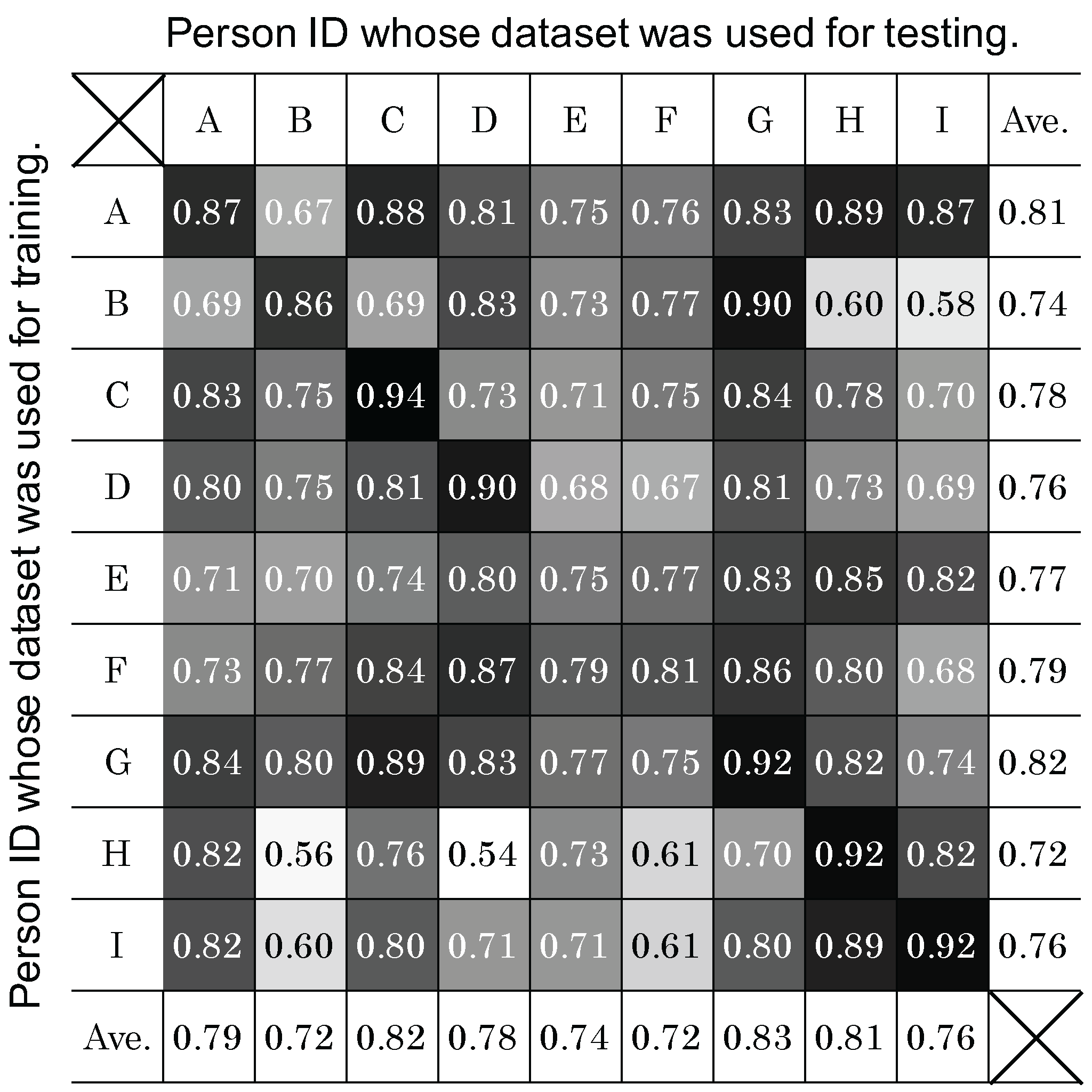
4.4. Person Dependency

4.4.1. Method

The classification performance shown in Section 4.2 was obtained by 10-fold cross-validation against the dataset from all subjects. This represents the average performance of the classification method. To evaluate the method under realistic conditions, where the data of a user are not used to train the classifier, we conducted leave-one-subject-out cross-validation (LOSO-CV). In LOSO-CV, the dataset of a particular subject is used for testing purposes, while the dataset of the rest of the subject group, i.e., eight subjects, is utilized for training a classifier. This process was iterated for all subjects, and an average was calculated.

It is not difficult to foresee that the best performance comes from using a personalized classifier, in which a classifier is trained with the dataset of a particular person and tested with the dataset of the same person (e.g., [26]). Therefore, to see the performance under this best condition, we conducted 10-fold cross-validation using personalized classifiers. This evaluation is referred to as self-CV.

4.4.2. Result and Analysis

Figure 10 shows the comparison in individual differences (Subjects A to I) and the averages for the two evaluation conditions. As shown in this figure, all subjects had equal or better classification performance with self-CV than with LOSO-CV. On average, self-CV performed better than LOSO-CV with an F-measure difference of 0.07.

The differences between the F-measure of self-CV and LOSO-CV for Subjects B, D and I are relatively large (0.11, 0.12 and 0.15, respectively). To analyze the reasons, a classifier was tuned for each subject. The classifiers were then tested with the datasets from other subjects. Figure 11 summarizes the resulting F-measures. In this table, the grayscale levels are normalized between the minimum (0.54) and the maximum (0.94) values to white and black, respectively. Furthermore, the values on the diagonal line of the same subject IDs indicate the F-measures of self-CV, shown also in the first row of Figure 10. As a result, we consider that “noisy” data are included in the LOSO-CV for Subjects B, D and I. In other words, some of the training data may have some subjects whose data were incompatible with Subjects B, D and I. In Figure 11, Subject H seems to be incompatible with Subjects B and D, as shown by the lowest values in each column (0.56 and 0.54, respectively). Furthermore, Subject B seems to be an incompatible subject for Subject I (0.58). To validate these thoughts, we built classifiers with datasets from “compatible” subjects as follows. First, an average of the F-measure excluding the self-CV value is calculated for each column. Then, the datasets of the subjects whose personalized classifiers performed better than the average are used to train a new classifier. Hence, Subjects C, D, E, F and G were selected as compatible subjects for Subject B, while Subjects A, B, E, F and G were selected as compatible subjects for Subject D. Similarly, as compatible subjects for Subject I, Subjects A, E, G and H were selected. As a result of testing with these new classifiers, the F-measures of LOSO-CV against Subjects B, D and I were improved to 0.80, 0.85 and 0.86, respectively; this was an increase of 0.05, 0.07 and 0.09 from the original LOSO-CV. In the future, we will investigate a method to find compatible persons to build a classifier in a systematic manner.

The F-measures of self-CV for Subjects E and F are relatively low, i.e., 0.75 and 0.81, respectively. This indicates that the features obtained from them failed to capture the characteristics of the target behaviors due to the large variation within subjects. Moreover, the average number of segments per class for Subjects E and F are 48 and 52, respectively, as calculated from Table 3. Therefore, the classifiers for these subjects are trained with around 44 and 47 segments (nine-tenths of the number of segments), respectively. We consider that these classifiers were not trained sufficiently.

4.5. Effect of Sensor Storing Position

4.5.1. Method

As investigated by Ichikawa et al. [27], people carry their smartphone terminals in various positions, such as their trousers pocket and chest pocket. We carried out an experiment to see the impact of storing position on the classification performance. The experiment was carried out by training a classifier with a dataset from a particular position and testing the classification with the datasets from the other positions.

4.5.2. Result and Analysis

Table 7. Robustness to storing position variation.

Trained with\Test with	(1)	(2)	(3)	(4)	Average
(1) Hand (texting)	0.86	0.82	0.82	0.91	0.86
(2) Trousers front pocket	0.85	0.85	0.86	0.89	0.86
(3) Trousers back pocket	0.83	0.85	0.88	0.88	0.86
(4) Chest pocket	0.86	0.83	0.80	0.91	0.85
Average	0.85	0.84	0.84	0.90	–

summarizes the F-measure results. In this table, the row indicates the storing positions from which datasets for training position-specific classifiers were obtained, and the column represents the datasets for testing. Note that the values on the diagonal line at the same positions were obtained by 10-fold cross-validation. These values indicate the ideal performance when classifiers are tuned for dedicated positions, and the average is 0.87. The table demonstrates that the classifiers tuned for particular positions did not predominantly perform best. This observation allows us to propose two approaches for constructing classification models.

The first approach is a straightforward one that constructs a single classifier with the datasets from all positions. This is the case shown in Section 4.2, and we obtain an F-measure of 0.89. This is better than the average of the tuned classifier approach (0.87). However, to realize this approach, datasets from all positions should be collected. The second approach is to share classifiers with some positions. In this case, a tuned classifier for the position “hand” is shared with the case in which the position of a terminal is judged as “chest pocket”, since the performance of “chest pocket” using a classifier tuned for “hand” is as high as with a tuned classifier for “chest pocket”. This can omit training data collection for the “chest pocket” classifier. Similarly, a classifier built from the dataset from “trousers back pocket” is shared with the data obtained from “trousers front pocket”. As shown in [26], front and back trousers pockets are often misrecognized for each other. Therefore, sharing the classifier between two positions can become robust against the mistake of the underlying storing position recognizer. In the second approach, the averaged F-measure is 0.88.

Table 8. Dealing with position dependency.

Approach	Average
(0) Tuned classifier for each position	0.87
(1) Single classifier with the dataset from all positions	0.89
(2) Sharing classifiers with some positions	0.88

summarizes the result. The second approach has a slightly worse F-measure; however, it just needs to collect the dataset from two positions, “hand” and “trousers back pocket”, which we consider a great advantage in reducing the cost of data collection. Such low-cost modeling accelerates the deployment of the system. The sharing approach may sacrifice the accuracy of recognition; however, it could be improved on the server side if a number of people utilized the system.

4.6. Robustness to Unknown Obstacle Size

4.6.1. Method

The performance evaluations above were performed by the classifiers trained by datasets with the obstacle sizes 0.2, 0.7 and 1.5 m. To understand the robustness against unknown sizes of obstacles, we used the datasets of obstacle sizes 0.5 and 1.0 m for the test, in which the dataset of obstacle sizes 0.2, 0.7 and 1.5 m was used to train the classifiers, as before.

4.6.2. Result and Analysis

The F-measures of the results are shown in

Table 9. Performance against unknown obstacle size.

Class	${\mathit{avoid}}_{\mathit{RL}}$	${\mathit{avoid}}_{\mathit{R}}$	${\mathit{avoid}}_{\mathit{LR}}$	${\mathit{avoid}}_{\mathit{L}}$	${\mathit{return}}_{\mathit{R}}$	${\mathit{return}}_{\mathit{L}}$	Average
F-measure	0.93	0.91	0.92	0.91	1.00	1.00	0.94

, where we can find that all values are better than the ones in the rightmost column in Table 6. We consider that this is because the obstacle size used for this test is in the range of the training dataset, i.e., 0.2 to 1.5 m. Therefore, the features obtained from the dataset with unknown obstacle sizes might fit into the ranges of trained features. The result implies that a classifier can be trained with a limited size of obstacles, i.e., probably for detecting upper, middle and lower sizes of obstacles.

5. Conclusions

In this article, we proposed a road anomaly detection system based on opportunistic sensing by using pedestrians’ smartphone terminals. Opportunistic sensing requires no explicit user involvement, which is expected to lower the barrier of people’s participation to the sensing activity. Although automatic road anomaly detection methods have already been proposed for cars and bikes, we considered that pedestrians’ avoidance behaviors are too slight to adapt these existing methods. After showing the overall system concept, we focused on the design of an obstacle avoidance behavior recognition system, in which waveform shaping, feature extraction and supervised classifiers were presented as major components. Six classes of avoidance behaviors were defined to test the recognition system from various aspects after collecting data from nine people with 410 trials on average. The following results were obtained:

• A 10-fold CV showed an average classification performance with an F-measure of 0.89 for six avoidance behaviors.
• The recognition system could handle the obstacle sizes of 0.2 to 1.5 m. Untrained sizes of obstacle avoidance were also recognized with an F-measure of 0.94.
• A user-independent classifier classified six avoidance behaviors with an F-measure of 0.81. The possibility of improving a user-independent classification by choosing classifiers trained by compatible persons was shown.
• Features resulting from (1) splitting a segment into the first half and the second half and (2) considering the monotonicity of change effectively recognized avoidance behaviors.
• The performance slightly depends on the sensor (smartphone) storing position on the body. Selecting a classifier for a particular position improves the performance. To reduce the cost of data collection, only the data from “hand” and “trousers back pocket” need be collected.

The results are obtained under an ideal and controlled environment; however, the results indicate that the proposed recognition method is robust against the size of obstacles and that the dependency on the storing position of a smartphone can be handled by an appropriate classifier per storing position. Furthermore, an analysis implies that classification of data from an “unknown” person can be improved by taking into account the compatibility of a classifier. The next step toward an all-in-one road anomaly detection system is to investigate an automatic avoidance event segmentation method that was performed by hand in this article. The key challenge is to discriminate normal behaviors that are associated with a change of walking direction, e.g., a pedestrian turns a corner or walks along a curved road, from true obstacle avoidance. We will leverage the characteristics in the azimuth difference and the walking distance to complete the change of walking direction to distinguish these situations. A real-world experiment is also required to assess the robustness of the proposed system. Lower-power operation is a critical issue for opportunistic sensing to be accepted by people because GPS-based positioning is generally a power-intensive approach [28]. Unlike continuous positioning, such as a noise map [29], our system can take an event-driven positioning, in which the positioning is performed only when an obstacle is detected. The challenge here is the positioning error due to the delay of activating a GPS receiver, i.e., the actual position of an avoidance event may be backward from the position where a GPS receiver returns. We will investigate a correction method by leveraging a pedestrian dead-reckoning (PDR) technology. Finally, server-side aggregation and the filtering technique will be investigated to realize the overall system.

References

1. City of Chiba. Chiba-Repo Field Trial: Review Report. 2013. Available online: http://www.city.chiba.jp/shimin/shimin/kohokocho/documents/chibarepo-hyoukasho.pdf (accessed on 30 September 2016).
2. mySociety Limited. FixMyStreet. Available online: http://fixmystreet.org (accessed on 30 September 2016).
3. Goldman, J.; Shilton, K.; Burke, J.; Estrin, D.; Hansen, M.; Ramanathan, N.; Reddy, S.; Samanta, V.; Srivastava, M.; West, R. Participatory Sensing: A Citizen-Powered Approach to Illuminating the Patterns that Shape Our World; Foresight and Governance Project, White Paper; Woodrow Wilson International Center for Scholars: Washington, DC, USA, 2009. [Google Scholar]
4. Lane, N.D.; Miluzzo, E.; Lu, H.; Peebles, D.; Choudhury, T.; Campbell, A.T. A survey of mobile phone sensing. IEEE Commun. Mag. 2010, 48, 140–150. [Google Scholar] [CrossRef]
5. Carrera, F.; Guerin, S.; Thorp, J.B. By the people, for the people: The crowdsourcing of “STREETBUMP”: An automatic pothole mapping app. ISPRS Int. Arch. Photogramm. Remote Sens. Spat. Inf. Sci. 2013, XL-4/W1, 19–23. [Google Scholar] [CrossRef]
6. Chen, D.; Cho, K.T.; Han, S.; Jin, Z.; Shin, K.G. Invisible Sensing of Vehicle Steering with Smartphones. In Proceedings of the 13th Annual International Conference on Mobile Systems, Applications, and Services (MobiSys ’15), Florence, Italy, 18–22 May 2015; pp. 1–13.
7. Eriksson, J.; Girod, L.; Hull, B.; Newton, R.; Madden, S.; Balakrishnan, H. The Pothole Patrol: Using a Mobile Sensor Network for Road Surface Monitoring. In Proceedings of the 6th International Conference on Mobile Systems, Applications, and Services (MobiSys ’08), Breckenridge, CO, USA, 17–20 June 2008; pp. 29–39.
8. Kaneda, S.; Asada, S.; Yamamoto, A.; Kawachi, Y.; Tabata, Y. A Hazard Detection Method for Bicycles by Using Probe Bicycle. In Proceedings of the IEEE 38th International Computer Software and Applications Conference Workshops (COMPSACW), Västerås, Sweden, 21–25 July 2014; pp. 547–551.
9. Mohan, P.; Padmanabhan, V.N.; Ramjee, R. Nericell: Rich Monitoring of Road and Traffic Conditions Using Mobile Smartphones. In Proceedings of the 6th ACM Conference on Embedded Network Sensor Systems (SenSys ’08), Raleigh, NC, USA, 4–7 November 2008; pp. 323–336.
10. Ishikawa, T.; Fujinami, K. Pedestrian’s Avoidance Behavior Recognition for Road Anomaly Detection in the City. In Proceedings of the ACM International Joint Conference on Pervasive and Ubiquitous Computing and ACM International Symposium on Wearable Computers (UbiComp/ISWC ’15), Osaka, Japan, 7–11 September 2015; pp. 201–204.
11. Bhoraskar, R.; Vankadhara, N.; Raman, B.; Kulkarni, P. Wolverine: Traffic and road condition estimation using smartphone sensors. In Proceedings of the IEEE Fourth International Conference on Communication Systems and Networks (COMSNETS), Bangalore, India, 3–7 January 2012; pp. 1–6.
12. Kamimura, T.; Kitani, T.; Kovacs, D.L. Automatic classification of motorcycle motion sensing data. In Proceedings of the IEEE International Conference on Consumer Electronics—Taiwan (ICCE-TW), Taipei, Taiwan, 26–28 May 2014; pp. 145–146.
13. Seraj, F.; van der Zwaag, B.J.; Dilo, A.; Luarasi, T.; Havinga, P.J.M. RoADS: A road pavement monitoring system for anomaly detection using smart phones. In Proceedings of the 1st International Workshop on Machine Learning for Urban Sensor Data, SenseML 2014, Nancy, France, 15 September 2014; pp. 1–16.
14. Thepvilojanapong, N.; Sugo, K.; Namiki, Y.; Tobe, Y. Recognizing bicycling states with HMM based on accelerometer and magnetometer data. In Proceedings of the SICE Annual Conference (SICE), Tokyo, Japan, 13–18 September 2011; pp. 831–832.
15. Iwasaki, J.; Yamamoto, A.; Kaneda, S. Road information-sharing system for bicycle users using smartphones. In Proceedings of the IEEE 4th Global Conference on Consumer Electronics (GCCE), Osaka, Japan, 27–30 October 2015; pp. 674–678.
16. Jain, S.; Borgiattino, C.; Ren, Y.; Gruteser, M.; Chen, Y.; Chiasserini, C.F. LookUp: Enabling Pedestrian Safety Services via Shoe Sensing. In Proceedings of the 13th Annual International Conference on Mobile Systems, Applications, and Services (MobiSys ’15), Florence, Italy, 18–22 May 2015; pp. 257–271.
17. Alessandroni, G.; Klopfenstein, L.C.; Delpriori, S.; Dromedari, M.; Luchetti, G.; Paolini, B.D.; Seraghiti, A.; Lattanzi, E.; Freschi, V.; Carini, A.; et al. SmartRoadSense: Collaborative Road Surface Condition Monitoring. In Proceedings of the 8th International Conference on Mobile Ubiquitous Computing, Systems, Servies and Technologies, Rome, Italy, 24–28 August 2014; pp. 210–215.
18. Tatebe, K.; Nakajima, H. Avoidance behavior against a stationary obstacle under single walking: A study on pedestrian behavior of avoiding obstacles (I). J. Archit. Plan. Environ. Eng. 1990, 418, 51–57. [Google Scholar]
19. Rabiner, L.R. A tutorial on hidden Markov models and selected applications in speech recognition. Proc. IEEE 1989, 77, 257–286. [Google Scholar] [CrossRef]
20. Hu, J.; Brown, M.K.; Turin, W. HMM based online handwriting recognition. IEEE Trans. Pattern Anal. Mach. Intell. 1996, 18, 1039–1045. [Google Scholar]
21. Wilson, A.D.; Bobick, A.F. Parametric Hidden Markov Models for gesture recognition. IEEE trans. Pattern Anal. Mach. Intell. 1999, 21, 884–900. [Google Scholar] [CrossRef]
22. Liu, J.; Zhonga, L.; Wickramasuriyab, J.; Vasudevanb, V. uWave: Accelerometer-based personalized gesture recognition, its applications. Pervasive Mob. Comput. 2009, 5, 657–675. [Google Scholar] [CrossRef]
23. Rajko, S.; Qian, G.; Ingalls, T.; James, J. Real-time gesture recognition with minimal training requirements and on-line learning. In Proceedings of the IEEE Conference on Computer Vision and Pattern Recognition, Minneapolis, MN, USA, 17–22 June 2007; pp. 1–8.
24. Machine Learning Group at University of Waikato. Weka 3—Data Mining with Open Source Machine Learning Software in Java. Available online: http://www.cs.waikato.ac.nz/ml/weka/ (accessed on 30 September 2016).
25. Witten, I.H.; Frank, E.; Hall, M.A. Data Mining: Practical Machine Learning Tools and Techniques, 3rd ed.; Morgan Kaufmann Publishers: San Francisco, CA, USA, 2011. [Google Scholar]
26. Fujinami, K.; Kouchi, S. Recognizing a Mobile Phone’s Storing Position as a Context of a Device and a User. In Proceedings of the 9th International Conference on Mobile and Ubiquitous Systems: Computing, Networking and Services (MobiQuitous), Beijing, China, 12–14 December 2012; pp. 76–88.
27. Ichikawa, F.; Chipchase, J.; Grignani, R. Where’s The Phone? A Study of Mobile Phone Location in Public Spaces. In Proceedings of the 2nd International Conference on Mobile Technology, Applications and Systems, Guangzhou, China, 15–17 November 2005; pp. 1–8.
28. Ben Abdesslem, F.; Phillips, A.; Henderson, T. Less is More: Energy-efficient Mobile Sensing with Senseless. In Proceedings of the 1st ACM Workshop on Networking, Systems, and Applications for Mobile Handhelds (MobiHeld ’09), Barcelona, Spain, 16–21 August 2009; pp. 61–62.
29. Rana, R.K.; Chou, C.T.; Kanhere, S.S.; Bulusu, N.; Hu, W. Ear-phone: An End-to-end Participatory Urban Noise Mapping System. In Proceedings of the 9th ACM/IEEE International Conference on Information Processing in Sensor Networks (IPSN ’10), Stockholm, Sweden, 12–15 April 2010; pp. 105–116.
Figure 1. Concept of the automatic road anomaly reporting system.
Ijgi 05 00182 g001
Figure 2. Definition of avoidance behavior.
Ijgi 05 00182 g002
Figure 3. Raw azimuth signals of a v o i d R (top), a v o i d R L (center) and r e t u r n R (bottom).
Ijgi 05 00182 g003
Figure 4. Avoidance behavior recognition flow.
Ijgi 05 00182 g004
Figure 5. Segmentation of a v o i d R L and a v o i d R .
Ijgi 05 00182 g005
Figure 6. Notations for f 8 and f 20 .
Ijgi 05 00182 g006
Figure 7. A scene of data collection.
Ijgi 05 00182 g007
Figure 8. Comparison of various supervised classifier models.
Ijgi 05 00182 g008
Figure 9. Classification performance with top-k contributing features. Features are provided in Table 1.
Ijgi 05 00182 g009
Figure 10. Individual differences in self-cross-validation (CV) and leave-one-subject-out cross-validation (LOSO-CV).
Ijgi 05 00182 g010
Figure 11. Applicability of person-dependent classification model.
Ijgi 05 00182 g011