Article

Spatiotemporal Variation of Precipitation Regime in China from 1961 to 2014 from the Standardized Precipitation Index

1
College of Earth Science and Resources, Chang’an University, Xi’an 710054, China
2
College of Land Engineering, Chang’an University, Xi’an 710054, China
3
Department of Crop & Soil Environmental Sciences, Virginia Tech, Blacksburg, VA 24061, USA
4
College of Geology Engineering and Geomatics, Chang’an University, Xi’an 710054, China
*
Author to whom correspondence should be addressed.
ISPRS Int. J. Geo-Inf. 2016, 5(11), 194; https://0-doi-org.brum.beds.ac.uk/10.3390/ijgi5110194
Submission received: 24 July 2016 / Revised: 12 October 2016 / Accepted: 23 October 2016 / Published: 27 October 2016

Abstract

:
Prediction of drought and flood events can be difficult, but the standardized precipitation index (SPI) calculated from monthly data may be a useful tool for predicting future dryness/wetness events in China. The rainy season SPI was calculated from monthly precipitation data from 3804 meteorological stations in China. The spatiotemporal variation, periodic change, and trend in rainy season SPI from 1961 to 2014 in eight regions were investigated. The results indicate that the rainy season SPI is valuable for assessing dryness/wetness spatial and temporal variations. The SPI time series in the northwest and southwest show increasing trends, while northeast China, south China, and Taiwan show more than one upward/downward trend during the study period, and the SPI time series in central, east, and north China show no change in trend. South China has an approximately 10-year periodic oscillation, while the other regions show an approximately 16-year periodic oscillation. The results of this study imply that the SPI can be used to explore historical drought/flood spatiotemporal variations, as well as to predict future wetness/dryness variations.

1. Introduction

Populations worldwide suffer from droughts and floods, which are considered the most widespread natural disasters in the world, causing extreme damage, but are difficult to predict [1,2,3]. Under a global warming scenario, droughts/floods will become even more serious problems [4]. Enhancing our ability to adapt to the adverse impacts of climate change is crucial for managing effective responses to future events, and requires accurate analysis of the duration, frequency, and intensity characterizing droughts and floods.
China has suffered from long-lasting droughts and frequent flooding, which have caused extreme damage to agriculture, and economic losses. Grain loss caused by drought accounts for up to 50% of total grain losses from 1950 to 1990 [5]. Abrupt changes in summer climate, which may be related to industrialization in east China, have been occurring since the early 1980s with a southward retreat of the summer monsoon rainy belt (SMRB). One natural disaster related to the SMRB is a climate patterns called the “northern drought with southern flooding” [6]. This phenomenon has been more significant since the end of the 1990s. For instance, in 2003, a flood occurred in the Huai River basin (central China), but the average rainfall was much lower than the long-term average in south China. Many regions in the east and northwest experienced substantial flooding in 2014, while some areas in the northeast of China experienced severe drought. In China, it is becoming more important to monitor and predict drought and flood events due to population increases, potential water shortages, as well as extreme weather events that are becoming more frequent with global warming.
A key requirement for drought monitoring and analysis is a quantitative description of dryness/wetness spatiotemporal variations, trend changes, and periodic changes. Extensive studies have been carried out to describe droughts. According to a review by Dai [4], droughts can be classified into three types:
  • Meteorological droughts, which occur when a region experiences months to years of less than normal precipitation.
  • Agricultural droughts, which occurs with either intense but less frequent rain events, evaporation levels above the long-term average, or when the soil becomes dry, all of which lead to reduced crop production and plant growth.
  • Hydrological droughts occur when river streamflow and water storage in aquifers, lakes, or reservoirs fall below long-term normal levels.
Over recent decades, researchers have described spatiotemporal variations in dryness/wetness changes using different drought indexes. For instance, Palmer [7] developed the Palmer Drought Index, sometimes called the Palmer drought severity index (PDSI), in 1965 to explore drought conditions in the Colorado River basin. PDSI is a measure of dryness based on recent precipitation and temperature, along with 66 other parameters [7,8]. PDSI has been proven the most effective index in determining long-term drought (over several months), but it is not as good with conditions lasting over a matter of weeks. Critics have complained that the utility of the Palmer Index is weakened by the arbitrary nature of Palmer’s algorithms, including the technique used for standardization. The Palmer Index’s inability to account for snow and frozen ground, as well as the relative complexity of the calculations, is also cited as a weakness.
A relatively simple drought Index called the standardized precipitation index (SPI) was developed in 1993 [9]. The SPI has many advantages over other traditional indices such as the PDSI. First, calculating the SPI is relatively simple, requiring only the precipitation parameter and not the land surface conditions, whereas 68 parameters are required to calculate the PDXI. The SPI has the additional advantage of a variable time scale; this versatility allows the SPI to monitor the short-term water supply, including soil moisture, which is important for agricultural production, and longer-term water resources such as groundwater, streamflow, and lake and reservoir levels. The third advantage of the SPI is that the frequencies of drought (extreme and severe) classifications for any location and any timescale are consistent because of the “standardized” nature, which promotes the quantitative comparison of drought incidence at different locations and different times. Thus, the SPI provides a better spatial standardization than the PDSI [8] for analyzing extreme drought events.
Given these advantages, the SPI has been widely used to monitor climatic conditions across different locations all over the world. A study in Europe calculated the 3, 6, 9, 12, 18, and 24 months SPI for the period 1901 to 1999 to study the time series of drought strength, number, mean duration, and maximum duration for a given location or region [9]. The SPI was introduced for analyzing droughts in Sicily from 1926 to 1996 [10]. A study comparing central eastern China, the north coast of Japan, and Korea found that occurrence of droughts was highly correlated in those three areas, but the time scales were different [11]. An analysis of different drought indexes was carried out to compare the SPI, PDSI, Palmer’s Z-index, and NOAA Drought Index (NDI) to determine the most appropriate index for monitoring agricultural drought on the Canadian prairies [12], and the results show that SPI is better correlated with the yield departures in the Canadian prairies than DPSI and NDI, and indicate that SPI is a good index for identifying agriculture drought. In Turkey, the SPI method was used to explore geographical variations of drought at multiple time steps [13]. Another study used the SPI to analyze the linkages between large-scale climate patterns and regional precipitation variability in the Colorado River basin [14].
The SPI has also been introduced in China to study drought, and has achieved significant results. For instance, the PDSI and SPI were calculated for 483 meteorological stations in China using monthly precipitation data from 1961 to 2005 for seven river basins to analyze the spatial distribution and trends in droughts [15]. Spatial and temporal variability of dry and wet periods in eastern China was analyzed based on the SPI [16]. Zhang et al. [17] evaluated drought events in XinJiang, China, using the SPI based on daily precipitation data from 53 stations from 1957 to 2009. Using monthly precipitation data from January 1951 to December 1998 from four locations in China, representing humid and arid climates, respectively, Wu et al. [18] compared the SPI, China-Z Index (CZI), and statistical Z-Score on 1 month, 3 months, 6 months, 9 months, and 12 months time scales. The result suggested that the SPI provided results similar to the CZI and Z-Score for all time scales. The SPI and aridity index were introduced to study observed changes in dryness/wetness episodes in the Pearl River basin, China, and the results showed that different wet and dry properties can be identified across the basin by the SPI [19].
The SPI has been used to study the spatial and temporal variations of dryness/wetness periods worldwide. However, macro-scale studies of these variations are very limited, with only a few studies having been made of the SPI in China, focusing on limited areas. Moreover, the periodic pattern of the SPI in China is not well identified. Therefore, the objectives of this study are:
  • To detect spatial and temporal variations in droughts/floods using the SPI for the entirety of China.
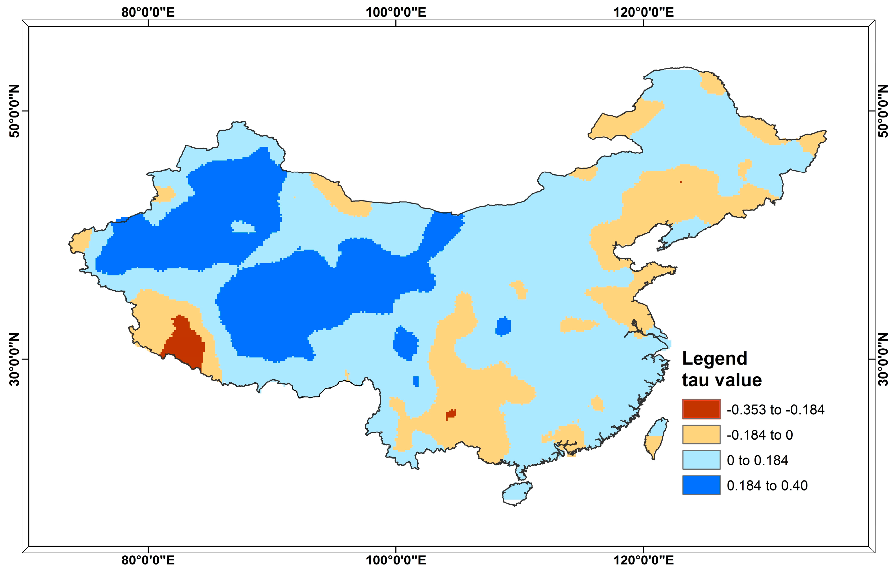
  • To analyze the spatial distribution of dryness/wetness trends using the Mann-Kendall nonparametric correlation test; specifically, to detect intensity trends in dry and wet events in eight regions in China from 1961 to 2014 using the sequential Mann-Kendall trend test.
  • To explore possible SPI periodic changes in eight districts of China by wavelet analysis.

2. Materials and Methods

2.1. Data Collection

Monthly precipitation data for China from 1961 to 2014 were obtained from the University of Delaware [20]. Monthly precipitation values in this dataset were derived from several station data resources, including a recent version of the Global Historical Climatology Network dataset (GHCN2), Atmospheric Environment Service/Environment Canada archive data, and data from the Hydro-meteorological Institute in St. Petersburg, Russia (courtesy of Nikolay Shiklomanov). Monthly values were derived from those archives that contained daily observations. From data within each daily station record, a monthly total precipitation was calculated when the number of missing days within a month was no more than five (station data resources and data presentation and calculation details can be found in the description file of this dataset [20]). Precipitation records in this dataset are normalized under the same standard, with the same spatial solution across the whole of China, and cover the whole study period (1961 to 2014) in each station, making this dataset a good candidate for wetness/dryness spatiotemporal variation analysis. The spatial resolution of the monthly precipitation data was 0.5° in latitude by 0.5° in longitude (Figure 1). In total, data from 3804 meteorology sites were collected to calculate the SPI values for China. The monthly mean precipitation in China from 1961 to 2014 shows that precipitation was mainly concentrated during the rainy season in all eight regions (from April to September, Figure 2). The variation and trend in precipitation anomaly time series from 1961 to 2014 were different among the eight regions in China (Figure 3).

2.2. SPI Calculation

Rainy season SPIs from 3804 stations were calculated to identify dryness/wetness spatiotemporal variations, trends, and periodic changes across eight stations in China. The SPI is the result of dividing the difference between the normalized rainy season precipitation and its seasonal mean from 1961 to 2014 by the standard deviation [9]. The SPI is based on statistical techniques, which can quantify the degree of wetness by comparing 1, 3, 6, 12, or 24-month rainfall totals with the historical rainfall period. According to a study, the six-month rainy season (from April to September) SPI is a good index to classify anomalously wet and dry conditions for the Pearl River basin [19]. In our study, the average monthly precipitation from 1961 to 2014 shows that precipitation was mainly concentrated during the rainy season (from April to September, Figure 2) in all eight regions in China. Therefore, we also choose the six-month rainy season SPI to analyze drought/flood conditions across the eight regions in China.
It is widely accepted that monthly precipitation time series very seldom fit a normal distribution. Therefore, to make the SPI follow a normal distribution, an initial transformation is usually done on the monthly precipitation data series. McKee et al. [9] originally used an incomplete gamma transformation to normalize the precipitation data. Lloyd-Hughes and Saunders [8] compared the gamma distribution and normal distribution, and found that the gamma distribution provided a better model for describing the monthly precipitation over most of Europe. A study in the Pearl River basin showed that a log-normal distribution had better performance in the rainy season (April to September), but the gamma distribution performed better in winter (January, February, and December) [19]. It should be noted that none of the transformations provided a better distribution at all sites. Based on Zhang et al.’s [19] conclusion, a log transformation was applied to the rainy season precipitation at all stations in this research. After the logarithmic transformation of the dataset, the sample mean and variance of the transformed data are u y ^ and σ y ^ , respectively, and the SPI can be calculated as Equation (1):
SPI = ln ( x i ) μ y σ y
where xi indicates the rainy season’s precipitation (i-th observation) at a climate station x.
Since the SPI is equal to the z-value of the normal distribution, Mckee et al. [9] proposed a seven-category classification for the SPI (Table 1). The SPI value provides a measure of the seriousness of the drought, and since it is normalized, this value is comparable from site to site and from year to year.

2.3. Mann-Kendall (MK) Correlation Test

The Mann-Kendall nonparametric correlation test [21] was used to test the SPI trend change at all 3804 climate stations in China from 1961 to 2014. For a given time series X (x1, x2, …, xn), the Mann-Kendall S statistic is computed as S = i = 1 n 1 j = i + 1 n s i g n ( T j T i ), where Tj and Ti are the SPI values for years j and i, j > i, respectively; while sign(TjTi) = 1 if (TjTi) > 0, sign(TjTi) = 0 if (TjTi) = 0, and sign(TjTi) = −1 if (TjTi) < 0. For n ≥ 10, the statistic S is approximately normally distributed with the mean E(S) = 0 and the variance (σ2) is defined as:
σ 2 = n ( n 1 ) ( 2 n + 5 ) t i ( i ) ( i 1 ) ( 2 i + 5 ) 18 ,
where t i denotes the number of ties to extend i. The statistic value, Kendall’s tau (τ), obtained by the Mann-Kendall test is a coefficient that measures the degree of concordance between the two ranked variables in the Mann-Kendall test [22]. Tau (τ) is essentially a scaled measure of S, and is described in Equation (2):
τ = S n ( n 1 ) / 2
where n denotes the number of concentration measurements (n = 54 in this study), τ ranges from −1 to 1, a trend is “strong” if the absolute value of τ is near 1, a negative τ value indicates a downward trend, and a positive τ value indicates an upward trend. Given a confidence level of α = 0.05, τ ≥ 0.184 indicates a significant upward trend and τ ≤ −0.184 indicates a significant downward trend.

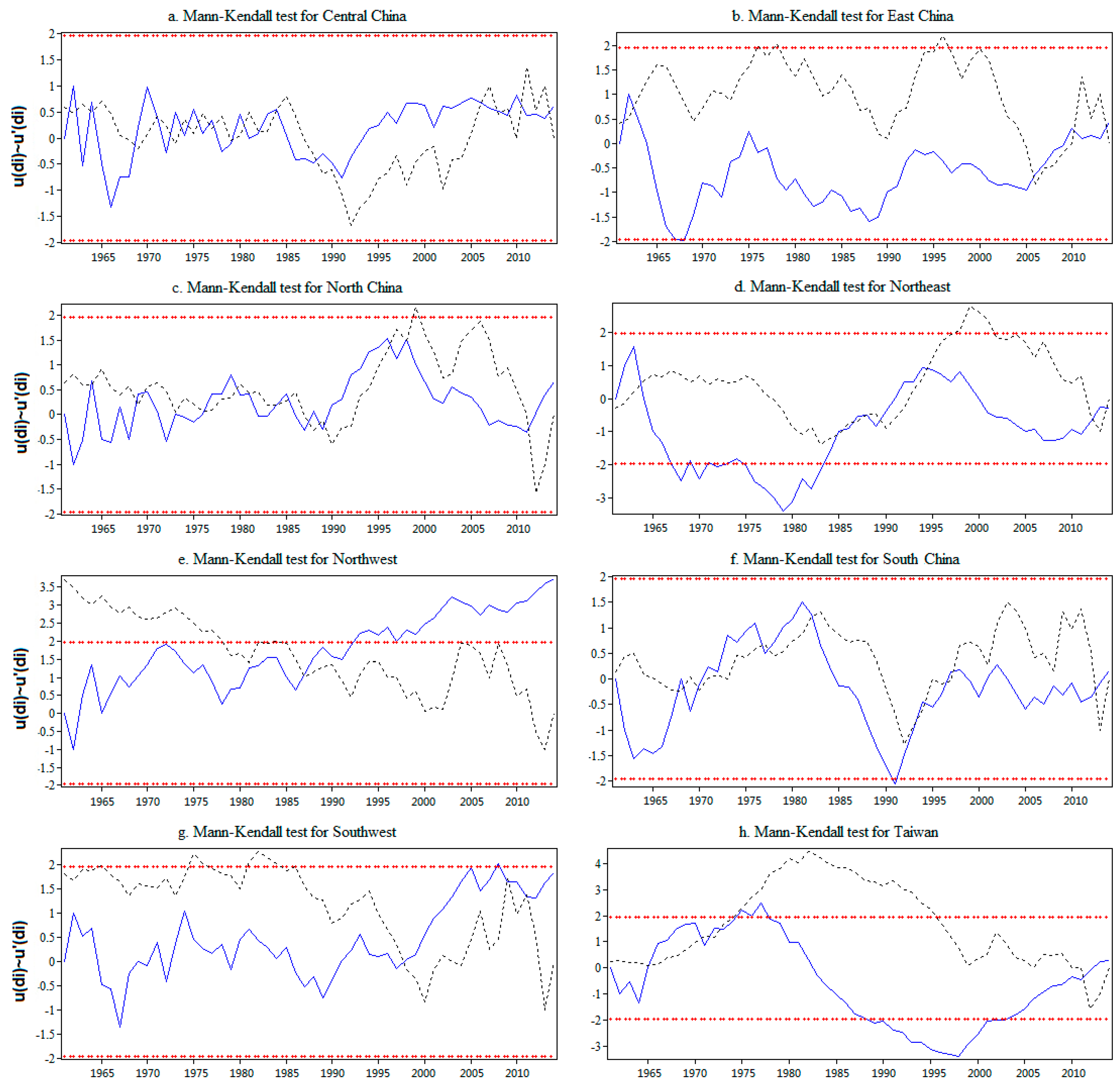
2.4. Sequential Mann-Kendall Test

The Mann-Kendall nonparametric correlation statistical method can test a monotonic trend at each site, but it cannot detect how wetness/dryness patterns change with time. To study how wetness/dryness changes over time in the eight regions in China, the Sequential Mann-Kendall test statistic was applied. We first aggregated the 3804 stations’ SPI time series to eight regions, and within each region, the sequential version of the Mann-Kendall test statistic, proposed by Sneyers [23], provides the benefit of giving all the statistical values of the time series data, and allows identification of the start time of the trend or change. This method has been widely applied in many research fields [24,25,26,27]. The sequential Mann-Kendall test calculates the ranked values of a given time series (x1, x2, x3, …, xn), and the magnitudes of yi (i = 1, 2, 3, …, n) are compared with yj (j = 1, 2, 3, …, i−1). For each comparison, the cases where yi > yj are counted and denoted by ni. A statistic di is calculated as d i = j = 1 i n i where the distribution of di has the mean E ( d i ) = i(i − 1)/4, and variance Var ( d i ) = i(i − 1)(2i + 5)/72. The sequential values of a standardized variable are calculated for each test statistic variable u(di) according to Equation (3):
u ( d i ) = d i E ( d ) V a r ( d i )
For a given confidence level (α = 0.05 in this study), if | u ( d i ) | 1.96 for a two-tail test, then the null hypothesis is rejected, implying a trend exists. A positive value indicates an upward (increasing) trend, and a negative value indicates a downward (decreasing) trend. The graphical representation of all u(di), 1 ≤ in, is denoted C1, also called a progressive series. In order to localize the beginning of the change, the same calculation procedure applied for the u(di) statistic is also applied to the retrograde series u’(di). The graphical representation of the retrograde series is C2. In the case of a significant trend, the intersection of C1 and C2 localizes the change and allows users to identify when the trend or change begins. In this study, the sequential Mann-Kendall test was applied to detect the SPI trend change and detect the beginning of change in eight regions in China, and Mann-Kendall’s tau statistic was used to test the monotonic trend of the SPI for all 3804 meteorology sites in China.

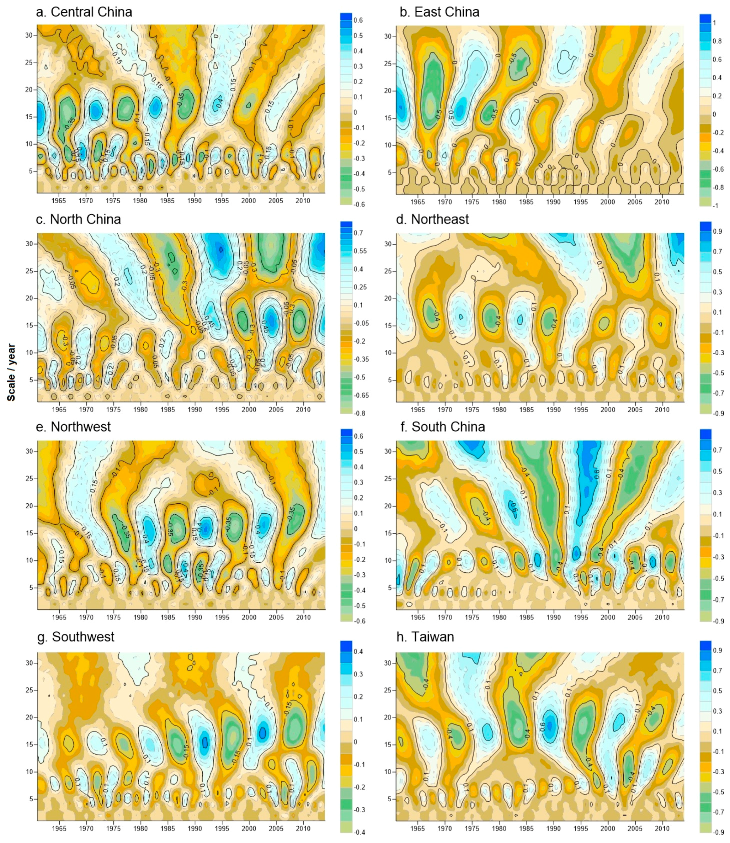
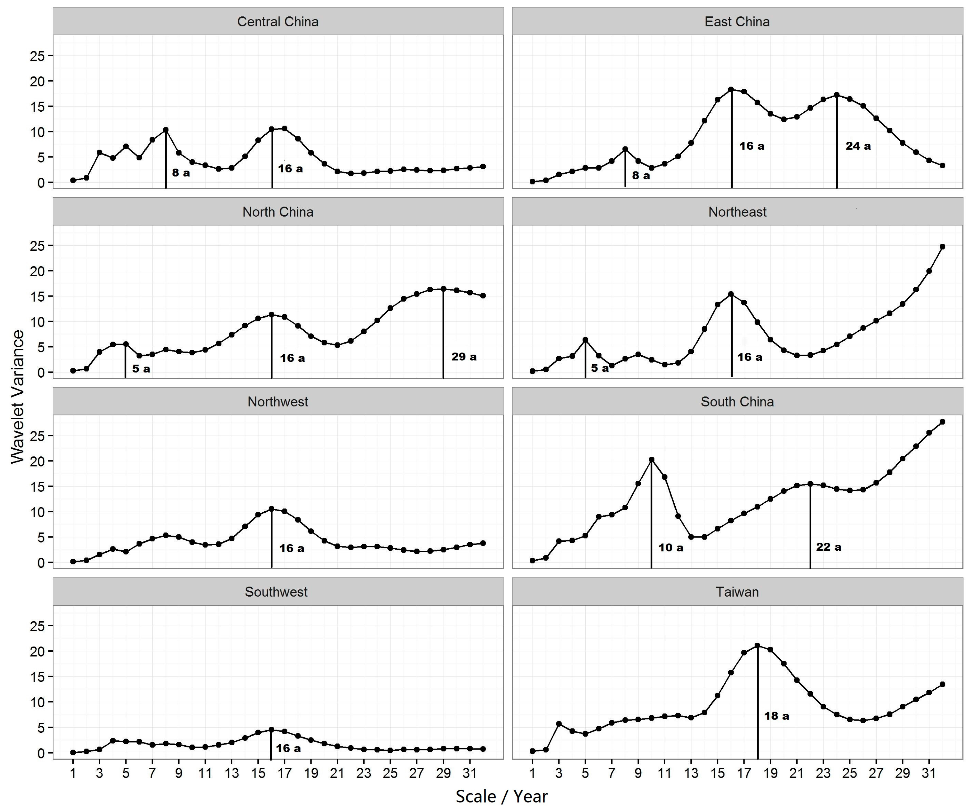
2.5. Wavelet Analysis

Wavelet analysis is a powerful tool for analyzing the periodic changes in a time series [25], which we utilized to examine periodic changes in SPI to analyze and predict future droughts in China. The basic idea of the wavelet transform is to represent or achieve a time series using the continuous wavelet transformation (CWT), defined as f ( t ) L 2 ( R ) and + f ( t ) d ( t ) = 0 . The CWT can be defined as the integral over all time of the real signal f(t) multiplied by the scaled, shifted versions of the wavelet function, which can be defined using Equation (4):
W f ( a , b ) = | a | 1 / 2 + f ( t ) ψ ¯ ( t b a ) d t
where ψ ¯ ( t b a ) is the complex conjugate function of the mother wavelet function ψ ( t b a ) , a is the scale variable defining the analysis window stretching, b is the time variable, and W f ( a , b ) is the CWT result of signal f(t).
The fundamental idea of CWT is to decompose a signal f(t) into wavelet coefficients as shown in Equation (4), thus the selection of wavelet functions is critical to wavelet analysis. The most common wavelet functions used in hydrology research are the Mexican hat wavelet, Haar wavelet, Daubechis wavelet, Morlet wavelet, and Mayer wavelet [21,28]. According to He et al. [29], the Morlet wavelet is given the phase and oscillation of the real part and imaginary part, and has a phase difference of π/2, which can eliminate false periodicities so that the results are more accurate. In this study, the complex Morlet wavelet was used to analyze the periodicity and variation tendency in the SPI time series for eight regions in China (the eight regions’ SPI time series were the same as in the Sequential Mann-Kendall test, which were aggregated from 3804 stations into eight regions). Within the Morlet wavelet, the function ψ (t) and wavelet variance Var(a) are defined as Equations (5) and (6):
ψ ( t ) = e i c t e t 2 / 2
V a r ( a ) = ( W f ) 2 ( a , b )
where c is a constant, and i denotes the imaginary part. The main period of the time series is obtained by the wavelet variance Var (a).

3. Results

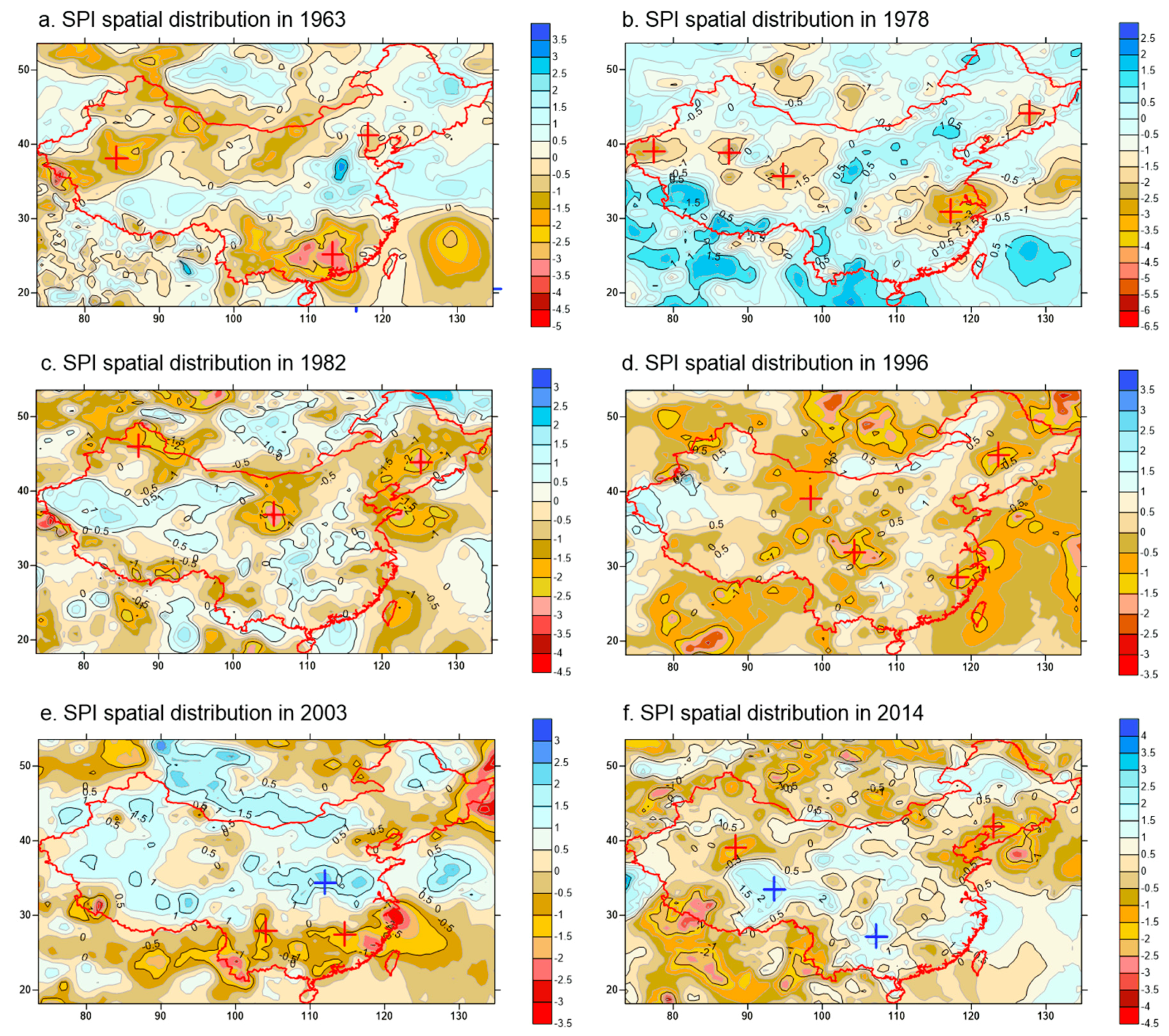
3.1. Spatiotemporal Variation of SPI in China

We used the SPI to represent the spatial distribution of wetness/dryness for 1963, 1978, 1982, 1996, 2003, and 2014 (Figure 4). To identify the spatial correlation of rainy SPI values in China, we first aggregated the monthly SPI time series (1961 to 2014) to yearly average, then we used the Moran’s I (‘ape’ package under R, version 3.1.3) to identify the spatial autocorrelation of rainy season SPI across China. The statistic result shows that rainy season SPI (average SPI value from 1961 to 2014) are highly spatial correlated across China (p value < 0.0001). Thus, the SPI spatial distribution was interpolated using the Kriging method in Surfer 10.0. We compared the spatial distribution of the SPI with the historical record of drought/flood events to identify how well the rainy season SPI can identify the spatial drought/flood variation. The rainy season SPI varied both spatially across China and with time, and covered six types of drought distributions classified by Wang et al. [5]: east-dispersed, east and west, north of the Yellow River, northwest and southeast, south of the Yellow River, and north of China (Table 2).
Our results show that the six-month (rainy season) SPI well describes the spatial distribution of droughts/floods in China as different drought types. In 1963, dryness was distributed in the southeast, northeast, and part of XinJiang Province (Figure 4a), which is consistent with historical drought records (Table 2). While wetness distributed in the north Yangtze River basin and south Yellow River basin (Figure 4a) in 1963, the “1963 extraordinary rainstorm” was reported in similar regions (Table 2). Droughts were widely dispersed from east to west in 1978 and 1996, and the SPI represented dryness from east to west as well (Figure 4b,d, and Table 2). In 1982, floods were distributed in the middle and lower reaches of the Yellow River (Table 2), where the SPI values show wetness (Figure 4c). Droughts were distributed in the middle and lower reaches of Yangtze River, north China, and the northeast (Table 2), where SPI values show dryness as well (Figure 4c). Notably, the “southern drought with northern flooding” events appeared in 2003 and the “northern drought with southern flooding” events appeared in 2014 (Table 2). Accordingly, the SPI values in 2003 show wetness centers in south China and the southeast but dryness in Huaihe River Basin (Figure 4e). The SPI values in 2014 show wetness in south China and the southeast but dryness in the northeast and XinJiang Province (Figure 4f).
Comparing the wetness/dryness spatial and temporal variation represented by the SPI (Figure 4) with historical drought/flood records (Table 2), we found that the rainy season SPI is a good index of drought/flood events.

3.2. Spatial Variance of SPI Trend in China

Results from Section 3.1 show that monthly precipitation can explain historical drought/flood events. We thus use rainy season SPI time series from 1961 to 2014 to analyze wetness/dryness trend in this study period. The Mann-Kendall nonparametric correlation test coefficient (τ) values of 3804 precipitation stations (Figure 5) indicate a regional heterogeneity to the trend in wetness/dryness that occurred in China Between 1961 and 2014. The Mann-Kendall correlation test indicates that most areas in east China show a non-significant upward or downward trend (Figure 5). However, in west China (northwest of Xinjiang Province, parts of Qinghai, and Tibet), the SPI shows a significant upward trend, and a downward trend appears in southwest Tibet and a small area in Yunnan Province (Figure 5). This indicates that the frequency of floods and droughts in these regions may be increasing.

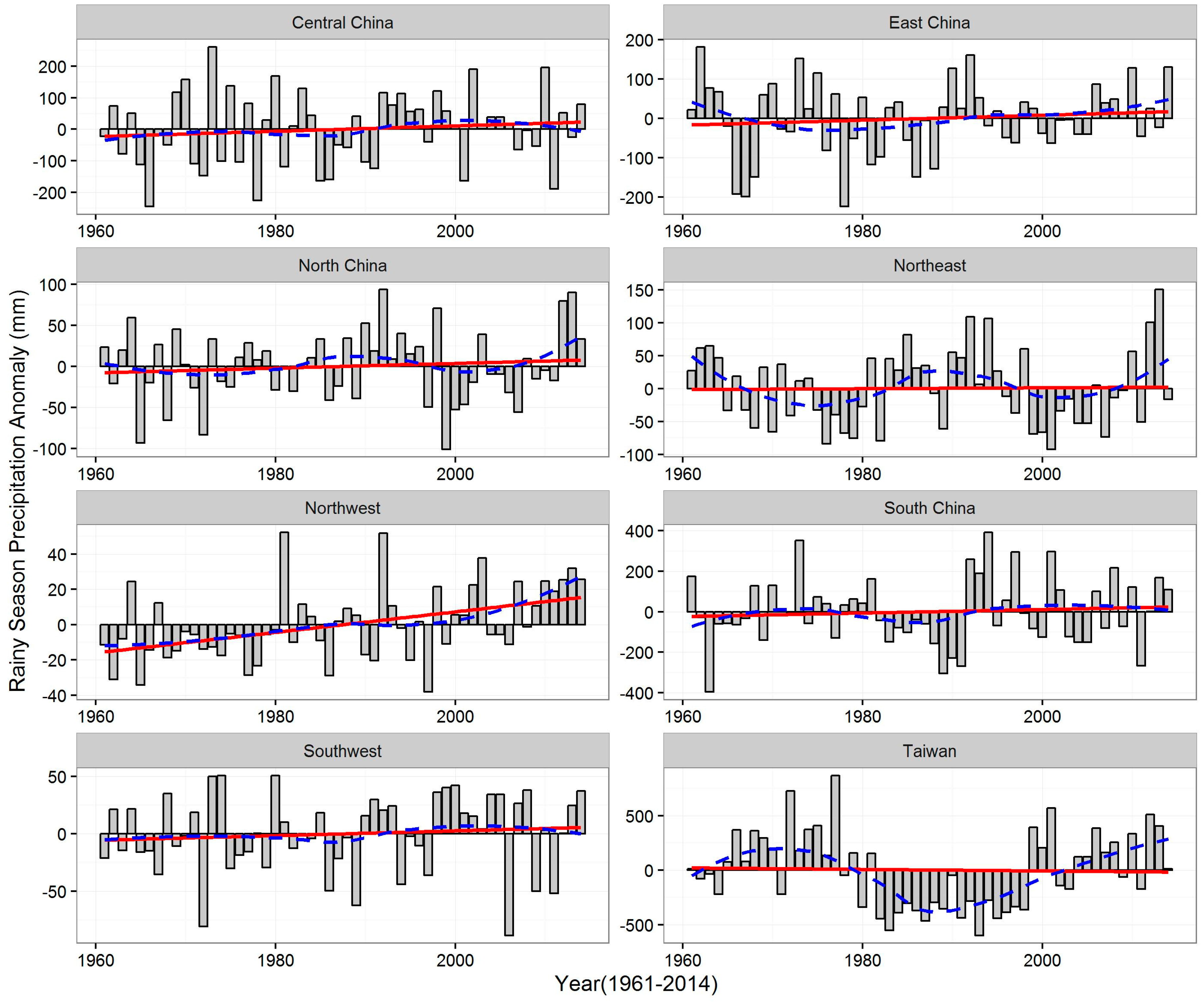
3.3. Temporal Trend of SPI in Eight Regions in China

As described by Sneyers [23], we detect the SPI time series possible change points in eight regions in China by comparing the progressive u(di) and retrograde u’(di) Mann-Kendall statistic variable values; if u(di) ≥ 1.96, then the null hypothesis is rejected, implying a trend exists. To avoid a type I error, we exclude any change point detected within the initial 10 years (from 1961 to 1970) and the last 10 years (from 2005 to 2014) of the time series. Analysis of the temporal trends in SPI indicates a regional pattern to how the wetness/dryness patterns are changing with time across the eight regions in China. In central China, east China, and north China, no trend is seen in the study period (Table 3 and Figure 6a–c, |u(di)| < 1.96 for all time). The SPI for northeast China exhibits a downward trend first (the change point is around 1963, but we exclude this change point because it occurs from 1961 to 1970), then shows an increase in 1985 (but not a significant increase, see Table 3 and Figure 6d). In 1994, the SPI began to decrease again (but not significantly). The SPI in the northwest shows a significant and continuously increasing trend beginning in 1986. The SPI for south China exhibits an upward (but not significant, Table 3 and Figure 6f) trend beginning around 1965 to 1982, then the SPI begins to decrease until 1993, when the SPI starts to increase again (but not significantly). In the southwest, the SPI was largely stable before 1997, but exhibited a significant increasing trend beginning in 1997 (Table 3 and Figure 6g). The SPI for Taiwan increased from the beginning until 1977 (the change point is around 1967, but we exclude this change point because it occurs within the first 10 years of the time series, see Table 3 and Figure 6h), then started a significantly decreasing trend until 1997 before increasing again, although not significantly.

3.4. Periodic Change in SPI across China

Periodic changes in the rainy season SPI time series was explored by wavelet analysis. The real part of the wavelet coefficient contour map (Figure 7) displays the periodic changes in SPI. Values of the real part of the wavelet coefficient > 0 indicate wet years, and values < 0 indicate drought years. The variation in the real part of the wavelet coefficient along different time scales (Y axis) demonstrates the oscillation of the time scale and reveals the domain predominant periods. The wavelet variance (Figure 8) displays the distribution of wavelet energy by scale, and is used to analyze the average period and oscillation variation in SPI in the eight districts in China. The first peak value has the strongest oscillation, and indicates the first main periodicity. The second and third peak values correspond to the second and third main periods, respectively.
Comparing eight regions in China, we found that the occurrence of wetness/dryness and oscillations were highly correlated across those eight regions. A common predominant 16-year periodicity is seen in all regions except north and south China, which exhibits a dominant 10-year and 29-year oscillation, respectively (Figure 7 and Figure 8). The common predominant periodicity of SPI time series change indicates that the oscillation of wetness/dryness may be related to some continental-scale climate phenomena that affect the precipitation pattern throughout China.
However, much heterogeneity is seen in the oscillation time scales and features across eight regions. In northwest, southwest China, as well as Taiwan, the SPI time series exhibit a single periodicity, while multiple periodicities are displayed in the other regions. In northeast and south China and Taiwan, a large-scale (more than 30-year) periodicity tends to appear, but this large-scale periodicity needs to be tested with a longer time series. In east China, a second (24-year) and third main period (8-year) is present besides the 16-year strongest oscillation (Figure 7 and Figure 8). The heterogeneity of the periodicity of SPI time series change illustrates that some regional scale factors also play an important role in affecting the wetness/dryness periodicity in China.

4. Discussion and Conclusions

Promoted by the societal need to better evaluate climate disasters (droughts and floods), as well as respond to water shortages, especially in consideration of increasing population levels and climate change, it becomes more and more crucial to evaluate spatiotemporal variations in the precipitation regime. Several studies have been performed using different climatic and hydrological indexes based on hydrological gauge stations’ monitoring data to explore spatial and temporal variations in wetness, dryness, stream flow, river sediments, and soil moisture in China [15,16,17,18,19,29]. Long-term and high-spatial-resolution climate data are crucial to analyze spatial and temporal variations in the precipitation regime. However, hydrological gauge stations in China are unevenly distributed spatially, with more stations installed in southern and eastern China, but fewer installed in western and northern China [15,16]. Another issue is that data record lengths vary among stations. Even worse, data from different stations are usually incompatible. These problems impede our ambition to clarify spatial and temporal variations in the precipitation regime.
In this study, we calculated SPI values based on a global monthly precipitation database, then analyzed the wetness/dryness spatiotemporal variation in eight regions based on the SPI values. Our results indicate that the SPI calculated based on the global monthly precipitation data well represent historical drought/flood disasters across China (Figure 4 and Table 2). Moreover, our results agree with many studies based on hydrological gauge stations. For example, using PDSI and SPI values calculated from 483 hydrological gauge stations in China, Zhai et al. [15] detected an upward dry trend in the Liaohe River basin and Haihei River basin from 1961 to 2005, which agrees with the trend found in this study (Figure 5). This study found a significant upward wetness trend in the northwest (Figure 5 and Figure 6e), similar to a result reported by Zhai et al. [15]. However, the PDSI indicates a statistically significant negative trend in the Songhua River basin [15], while this study detected a wetness trend (although not a significant one, Figure 5) in most areas of the Songhua River basin. One possible cause for this difference is that the station density is much higher in this study than in Zhai et al. [15]; a second possibility is that Zhai et al. [15] used the PDSI as the wetness/dryness indicator, while this study used the SPI to represent the wetness/dryness spatiotemporal variation. Using rain gauge data, Bordi et al. [16] analyzed the wet and dry spatiotemporal variability in eastern China and found 24-year, 16-year, and 4-year periodicities, which agree with the periodicities (24-year, 16-year, and 8-year) found in this study in the same region. Zhang et al. [17] presented the spatial and temporal drought variation from 1957 to 2009 using 53 rain gauge stations in XinJiang Province, and found that droughts tend to be weakening in the entire XinJiang region. In this study, we also detected a significant upward wetness trend for most of the XinJiang region (Figure 5). In the Pearl River basin, drought/wetness episodes from 1960 to 2005 were analyzed based on SPI calculated from 42 rain stations, and the western part of the Pearl River basin was found to be wetter, and the southern part to be dryer [19]. In this study, we detected exactly the same trends in the same region (Figure 5).
The results of this study are very consistent with previous research based on rain gauge stations, which demonstrated that global monthly precipitation data can be used to explore wetness/dryness spatiotemporal variations in China and other regions. Considering its high spatial resolution (0.5° latitude × 0.5° longitude) and record length (from 1900 to the present, with continuous updating), this data source is a good candidate for reconstructing historical wetness/dryness spatiotemporal variations and for better predicting future climate-related disasters (drought and floods). Building a record of historical drought and flood disaster events in China is helpful to better understand the spatiotemporal variations in drought and flooding, and for future drought and flood monitoring in China. This research provides a relatively simple precipitation index that can be used to explain the occurrence of historical drought/flood events, as well as to identify the trend changes and periodic patterns of wetness/dryness changes, which can be useful for future drought and flood monitoring. Since precipitation records in China have a long history, the SPI can be introduced to construct a database of drought and flood disaster events in China for future study. The SPI can also be a good index for flood risk monitoring. For instance, Du et al. [26] used the SPI for flood monitoring in Hunan Province, China. Seiler et al. [27] used the SPI to detect flood risk in the southern part of Cordoba Province in Argentina. However, the SPI is less frequently used to monitor floods than to study droughts, and continental or global-scale applications of the SPI for flood monitoring are not conducted.
A common predominant periodicity of around 16 years was detected for all regions except for northern and southern China (Figure 7 and Figure 8), which indicates that the oscillation of wetness/dryness may be related to some global or continental-scale climate phenomena that effect the precipitation pattern throughout China. Using data from the National Center for Atmospheric Research/National Centers for Environmental Prediction (NCAR/NCEP), Zhang et al. [19] found that the upward wetness trend in the rainy season is influenced by the moisture content in the air and water vapor. Mantua and Hare [30] described the Pacific Decadal Oscillation (PDO) and indicated that this long-lived EI Niño-like pattern of Pacific climate variability has a distinct effect on spatial and temporal precipitation patterns in the Southern Hemisphere, the mid-latitude South Pacific Ocean, Australia, and South America. Furthermore, a 15–25 years and 50–70 years oscillation were detected in the PDO variation. Using PDO data from 1951 to 1998, Zhu and Yang [31] found that the decadal climate pattern in China is closely related to the PDO change. More specifically, during a “warm” PDO regime period, northeastern and northern China and the Yangtze River valley are drier, but those regions become wetter during the “cool” PDO regime period. The 16-year periodicity detected in this study may be related to the 15–25 years “warm” and “cool” period variation. According to Wang and Zhao [32], a 36-year atmospheric circulation affects the drought/flood periodicity and climate pattern in China. Wavelet analysis of the SPI time series in this study shows that a periodicity longer than 30 years may exist in northeastern and southern China and Taiwan. This large-scale oscillation may be related to the 36-year atmospheric circulation oscillation; however, longer time series data are required to detect this large-scale periodicity.
Some differences in the oscillation time scales and features were widely detected among the eight regions in China. In central, eastern, northern, and northeast China, a periodicity of less than 10 years is seen. This may be related to the EI Niño phenomenon, which has a two to seven years cycle [33]. A study found hydrographic and biological anomalies in the South China Sea related to the EI Niño event [33]. Another study found that the EI Niño–South Oscillation (ENSO) strongly influences extreme events such as floods and droughts River basin [34]. It should also be noted that the dryness/wetness periodic changes depend on the time scale of SPI (e.g., 1, 3, 6, …, 24 months SPI), thus the oscillation period represented by wavelet analysis may vary when the SPI time scale changes. Therefore, more study is needed to clarify the uncertainty of predictions influenced by the SPI time scale.
Trends in the precipitation regime represented by the SPI clearly change from region to region in China. The northwest shows a continuous upward wetness trend in the study period, but central China, east China, and north China show no trend, and other regions show both upward and downward wetness trends in different periods (Table 3 and Figure 6). The heterogeneity of the SPI trend in different regions may be related to the fact that the response of regional rainfall to global climate change is spatially variable [35]. It may also be related to human activity, such as the “Grain for Green” program, which promoted significant vegetation coverage in the Yellow River basin from 1982 to 1999 [36]. The total forest biomass increases slightly in north China, but decreases in south central and east China [37], and the SPI series also shows a relatively flat pattern in north China, but has decreased in south China since 1982 (but not significantly, see Table 3 and Figure 6). In the southwest, where the forest biomass decreased from 1949 to 1976 then increased from 1977 to 1998 [37], a similar wetness trend was found in the southwest according to the SPI in this study; it remained unchanged from 1961 to 1997, then increased after 1997 (but not significantly, see Table 3 and Figure 6). These agreements between land-use change and wetness/dryness trends across different regions indicate that human activity may potentially influence spatial variability and trends in wetness/dryness. However, more research needs to be conducted to clarify the magnitude and mechanism of how human activity affects spatiotemporal variations in wetness/dryness in China.
The SPI time series in China shows spatial variability (Figure 5 and Figure 6), such as the “southern drought and northern flooding” in 2003 or “southern flooding and northern drought” in 2014 (Figure 3 and Table 2). Similarly, using monthly precipitation data from 160 stations from 1951 to 2000, Bordi et al. [16] analyzed the spatial structure of wetness/dryness variations and found that when wetness was found in the east, dry conditions were usually observed in southern China, and vice versa. A study by Xu [6] pointed out that this type of spatial variation in precipitation is related to southward movement of the summer monsoon, and the main cause of this phenomenon may not be purely natural climate change but the acceleration of industrialization in east China, which emits large amounts of sulfur dioxide.
In conclusion, global warming and industrialization have resulted in a worsening climate in China over the past several decades. For instance, climate change may also be related to the detected decline in soil moisture over the last three decades in north China [38]. Southward retreat of the summer monsoon rainy belt has resulted in a new pattern of drought and flood (i.e., “northern drought with southern flooding” in China). Such phenomena not only make it more difficult to monitor droughts and flooding, but also complicate implementation of adaptive responses to extreme events. This research indicates that the six-month SPI calculated based on precipitation during the rainy months well represents the spatial distribution of droughts and floods in China. Analyses of the SPI trend and spatial and temporal oscillations provide a valid method for future drought/flood forecasting, which could help us adapt to the adverse impacts of climate change.

Acknowledgments

This research was supported by the Chinese Universities Scientific Fund (No. 310827161019). We greatly appreciate Meredith K. Steele, who participated in revising the article for important intellectual content, and reviewers who provided many constructive comments that greatly improved the manuscript.

Author Contributions

Xuefeng Yuan conceived and designed the experiments, calculated and analyzed the data, and wrote the paper; Jinshi Jian and Gang Jiang performed the data integration and data analysis, and wrote part of the paper.

Conflicts of Interest

The authors declare no conflict of interest. The founding sponsors had no role in the design of the study, in the collection, analyses, and interpretation of the data, in the writing of the manuscript, or in the decision to publish the results.

References

  1. Jongman, B.; Wagemaker, J.; Romero, B.; De Perez, E. Early flood detection for rapid humanitarian response: Harnessing near real-time satellite and twitter signals. ISPRS Int. J. Geo-Inf. 2015, 4, 2246–2266. [Google Scholar] [CrossRef]
  2. Forsythe, K.W.; Schatz, B.; Swales, S.J.; Ferrato, L.J.; Atkinson, D.M. Visualization of lake mead surface area changes from 1972 to 2009. ISPRS Int. J. Geo-Inf. 2012, 1, 108–119. [Google Scholar] [CrossRef]
  3. De Sherbinin, A.; Chai-Onn, T.; Jaiteh, M.; Mara, V.; Pistolesi, L.; Schnarr, E.; Trzaska, S. Data integration for climate vulnerability mapping in West Africa. ISPRS Int. J. Geo-Inf. 2015, 4, 2561–2582. [Google Scholar] [CrossRef]
  4. Dai, A. Drought under global warming : A review. Wires Clim. Chang. 2011, 2, 45–65. [Google Scholar] [CrossRef]
  5. Wang, J.; Sun, H.; Xu, W.; Zhou, J. Spatio-temporal change of drought disaster in China in recent fifty years. J. Nat. Disaster 2011, 11, 1–6. [Google Scholar]
  6. Xu, Q. Abrupt change of the mid-summer climate in central east China by the influence of atmospheric pollution. Atmos. Environ. 2001, 35, 5029–5040. [Google Scholar] [CrossRef]
  7. Palmer, W.C. Meteorological Drought; US Weather Bureau: Washington, DC, USA, 1965.
  8. Lloyd, H.B.; Saunders, M.A. A drought climatology for Europe. Int. J. Climatol. 2002, 22, 1571–1592. [Google Scholar] [CrossRef]
  9. Mckee, T.B.; Doesken, N.J.; Kleist, J. The relationship of drought frequency and duration to time scales. In Proceedings of the Eighth Conference on Applied Climatology, Anaheim, CA, USA, 17–23 January 1993.
  10. Bonaccorso, B.; Bordi, I.; Cancelliere, A.; Rossi, G.; Sutera, A. Spatial variability of drought : An analysis of the SPI in Sicily. Water Resour. Manag. 2003, 17, 273–296. [Google Scholar] [CrossRef]
  11. Min, S.K.; Kwon, W.T.; Park, E.H.; Choi, Y. Spatial and temporal comparisons of droughts over Korea with East Asia. Int. J. Climatol. 2003, 23, 223–233. [Google Scholar] [CrossRef]
  12. Quiring, S.M.; Papakryiakou, T.N. An evaluation of agricultural drought indices for the Canadian prairies. Agric. For. Meteorol. 2003, 118, 49–62. [Google Scholar] [CrossRef]
  13. Sönmez, F.K.; Kömüscü, A.Ü.; Erkan, A.; Turgu, E. An analysis of spatial and temporal dimension of drought vulnerability in Turkey using the standardized precipitation index. Nat. Hazards. 2005, 35, 243–264. [Google Scholar] [CrossRef]
  14. Kim, T.; Valde, J.B.; Nijssen, B.; Roncayolo, D. Quantification of linkages between large-scale climatic patterns and precipitation in the Colorado River Basin. J. Hydrol. 2006, 321, 173–186. [Google Scholar] [CrossRef]
  15. Zhai, J. Spatial variation and trends in PDSI and SPI indices and their relation to streamflow in 10 large regions of China. J. Clim. 2010, 23, 649–663. [Google Scholar] [CrossRef]
  16. Bordi, I.; Fraedrich, K.; Jiang, J.M.; Sutera, A. Spatio-temporal variability of dry and wet periods in eastern China. Theor. Appl. Climatol. 2004, 79, 81–91. [Google Scholar] [CrossRef]
  17. Zhang, Q.; Li, J.; Singh, V.P.; Bai, Y. SPI-based evaluation of drought events in Xinjiang, China. Nat. Hazards. 2012, 64, 481–492. [Google Scholar] [CrossRef]
  18. Wu, H.; Hayes, M.J.; Weiss, A.; Hu, Q. An evolution of the standardized precipitation index, the China-Z index and the statistical Z-score. Int. J. Climatol. 2001, 21, 745–758. [Google Scholar] [CrossRef]
  19. Zhang, Q.; Xu, C.Y.; Zhang, Z. Observed changes of drought/wetness episodes in the Pearl River basin, China, using the standardized precipitation index and aridity index. Theor. Appl. Climatol. 2009, 98, 89–99. [Google Scholar] [CrossRef]
  20. Willmott, C.J.; Matsuura, K.; Legates, D.R. Terrestrial Air Temperature and Precipitation: Monthly and Annual Time Series (1950–1999); University of Delaware: Newark, DE, USA, 2001. [Google Scholar]
  21. Jian, J.; Jiao, J.; Du, X.; Ma, L. Runoff and sediment dynamics and driving factors in the Jiaoqiao hydrological station of Nunkiang River. Bull. Soil Water Conserv. 2011, 31, 15–21. [Google Scholar]
  22. Best, D.J.; Gipps, P.G. The upper tail probabilities of Kendall’s tau. J. R. Stat. Soc. 1974, 23, 98–100. [Google Scholar]
  23. Sneyers, R. On the statistical analysis of series of observations. In Technical Note—World Metrological Organization; World Meteorological Organization: Geneva, Switzerland, 1990; pp. 1–192. [Google Scholar]
  24. Chatterjee, S.; Khan, A.; Barman, N.K. Research article application of sequential Mann-Kendall test for detection of approximate significant change point in surface air temperature for Kolkata weather observatory, west Bengal, India. Int. J. Curr. Res. 2014, 6, 5319–5324. [Google Scholar]
  25. Wei, Y.; Jiao, J.; Zhao, G.; Zhao, H.; He, Z.; Mu, X. Spatial–temporal variation and periodic change in streamflow and suspended sediment discharge along the mainstream of the Yellow River during 1950–2013. Catena 2016, 140, 105–115. [Google Scholar] [CrossRef]
  26. Du, J.; Fang, J.; Xu, W.; Shi, P. Analysis of dry/wet conditions using the standardized precipitation index and its potential usefulness for drought/flood monitoring in Hunan Province, China. Stoch. Environ. Res. Risk Assess. 2013, 27, 377–387. [Google Scholar] [CrossRef]
  27. Seiler, R.A.; Hayes, M.; Bressan, L. Using the standardized precipitation index for flood risk monitoring. Int. J. Climatol. 2002, 22, 1365–1376. [Google Scholar] [CrossRef]
  28. Li, C.H.; Yang, Z.F.; Huang, G.H.; Li, Y.P. Identification of relationship between sunspots and natural runoff in the Yellow River based on discrete wavelet analysis. Expert Syst. Appl. 2009, 36, 3309–3318. [Google Scholar] [CrossRef]
  29. He, B.; Miao, C.; Shi, W. Trend, abrupt change, and periodicity of streamflow in the mainstream of Yellow River. Environ. Monit. Assess. 2013, 185, 6187–6199. [Google Scholar] [CrossRef] [PubMed]
  30. Mantua, N.J.; Hare, S.R. The pacific decadal oscillation. J. Oceanogr. 2002, 58, 35–44. [Google Scholar] [CrossRef]
  31. Zhu, Y.; Yang, X. Relationships between pacific decadal oscillation (PDO) and climate variabilities in China. Acta Meteorol. Sin. 2003, 61, 641–654. [Google Scholar]
  32. Wang, S.; Zhao, Z. The 36-yr wetness oscillation in China and its mechanism. Acta Meteorol. Sin. 1979, 37, 64–73. [Google Scholar]
  33. Tseng, C.M.; Liu, K.K.; Wang, L.W.; Gong, G.C. Anomalous hydrographic and biological conditions in the northern South China Sea during the 1997–1998 El Nino and comparisons with the equatorial Pacific. Deep Sea Res. Part I Oceanogr. Res. Pap. 2009, 56, 2129–2143. [Google Scholar] [CrossRef]
  34. Wang, Z.; Wei, G.; Chen, J.; Liu, Y.; Ma, J.; Xie, L.; Deng, W.; Ke, T. El Niño–Southern Oscillation variability recorded in estuarine sediments of the Changjiang River, China. Quat. Int. 2016. [Google Scholar] [CrossRef]
  35. Huang, P.; Xie, S.P.; Hu, K.; Huang, G.; Huang, R. Patterns of the seasonal response of tropical rainfall to global warming. Nat. Geosci. 2013, 6, 357–361. [Google Scholar] [CrossRef]
  36. Yang, S.; Liu, C.; Sun, R. The vegetation cover over the last 20 years in Yellow River basin. Acta Geogr. Sin. 2002, 57, 679–684. [Google Scholar]
  37. Fang, J.; Chen, A.; Peng, C.; Zhao, S.; Ci, L. Changes in forest biomass carbon storage in China between 1949 and 1998. Science 2001, 292, 2320–2322. [Google Scholar] [CrossRef] [PubMed]
  38. Liu, Y.; Pan, Z.; Zhuang, Q.; Miralles, D.G.; Teuling, A.J.; Zhang, T.; An, P.; Dong, Z.; Zhang, J.; He, D.; et al. Agriculture intensifies soil moisture decline in Northern China. Sci. Rep. 2015, 5, 11261. [Google Scholar] [CrossRef] [PubMed] [Green Version]
Figure 1. Research area and spatial distribution of precipitation across eight regions in China: central China (CC), east China (EC), north China (NC), northeast (NE), northwest (NW), south China (SC), southwest (SW), and Taiwan (TW).
Ijgi 05 00194 g001
Figure 2. Monthly mean precipitation for the period 1961 to 2014 in eight regions in China: central China, east China, north China, northeast, northwest, south China, southwest, and Taiwan.
Ijgi 05 00194 g002
Figure 3. Trend in rainy season (April to September) precipitation anomaly (difference between annual precipitation and long-term average precipitation) from 1961 to 2014 across central China, east China, north China, northeast, northwest, south China, southwest, and Taiwan. Red solid lines indicate linear trend in precipitation anomaly time series, and dashed blue lines show Local Polynomial Regression Fitting (loess regression in R) of rainy season precipitation anomaly.
Ijgi 05 00194 g003
Figure 4. Spatial distribution of six-month (rainy season: April to September) SPI across China in 1963, 1978, 1982, 1996, 2003, and 2014. Red crosses indicate drought locations, while blue crosses indicate flood locations. SPI spatial distribution was interpolated using Kriging method in Surfer 10.0. (a) SPI spatial distribution in 1963; (b) SPI spatial distribution in 1978; (c) SPI spatial distribution in 1982; (d) SPI spatial distribution in 1996; (e) SPI spatial distribution in 2003; (f) SPI spatial distribution in 2014.
Ijgi 05 00194 g004
Figure 5. Spatial distribution of Mann-Kendall test tau value of SPI time series for all 3804 stations from 1961 to 2014 in China. Tau ≤ −0.184 indicates a significant downward trend, −0.184 ≤ tau ≤ 0 indicates a downward but not significant trend; 0.0 < tau < 0.184 indicates an upward but not significant trend; tau ≥ 0.184 indicates a significant upward trend.
Ijgi 05 00194 g005
Figure 6. Sequential Mann-Kendall test for SPI time series from 1961 to 2014 in (a) central China; (b) east China; (c) north China; (d) northeast; (e) northwest; (f) south China; (g) southwest; (h) Taiwan. Blue line denotes SPI progressive series, black dotted line is retrograde series, red dotted line indicates 95% confidence interval (u = 1.96 or u = −1.96).
Ijgi 05 00194 g006
Figure 7. Wavelet coefficient counter map of SPI in China for 1961–2014 in (a) central China; (b) east China; (c) north China; (d) northeast; (e) northwest; (f) south China; (g) southwest; and (h) Taiwan.
Ijgi 05 00194 g007
Figure 8. Variance of Morlet wavelet transform coefficients for SPI time series in east China, north China, northeast, northwest, south China, southwest, and Taiwan from 1961–2014.
Ijgi 05 00194 g008
Table 1. Standardized precipitation index (SPI) categories based on initial classification of SPI values.
CategorySPIProbability (%)
Extremely wet2.00 and above2.3
Severely wet1.50 to 1.994.4
Moderately wet1.00 to 1.499.2
Near normal−0.99 to 0.9968.2
Moderate drought−1.00 to −1.499.2
Severe drought−1.50 to −1.994.4
Extreme drought−2.00 and less2.3
Table 2. A synthesized summary of drought and flood disaster (and type) distribution in China in 1963, 1978, 1982, 1996, 2003, and 2014.
Year and Types of DroughtDroughtFlood
1963
(East Dispersed)
South of Yangtze River; southwest and south of China; south, middle, and west of Hunan Province; Huizhou City in Guangdong Province, and most areas of Guangxi Province suffered from severe drought. North China Plain; south of Henan Province, and west of the Haihe River basin. The “1963 extraordinary rainstorm” extended from north of Henan to Baoding in Hebei, from Jing-Guang railroad to the border between Hebei and Shanxi Province.
1978
(East and west)
Middle and lower reaches of Yangtze River.Part of Sichuang, Guizhou, Guangdong, Hunan, and Gansu Province.
1982
(North of Yellow River)
Middle and lower reaches of Yangtze River, north China, and northeast. Middle and lower reaches of Yellow River; Approximately 173,000 hm2 agricultural lands destroyed by flood.
1996
(Northwest and Southeast)
Northwest and southeast of China.Middle reaches of Yangtze River and part of Hanjiang River basin.
2003
(South of Yellow River)
South of China, part of the southwest; part of Hunan, Jiangxi, Zhejiang, Fujian, and Guangdong experienced drought in autumn and winter. Huaihe River Basin’s average rainfall was 2.2 times the annual average; 30 days of > 400 mm rainfall recorded in all areas except the Niufushan region in the Huaihe River Basin.
2014
(South Flood, north drought)
Henan Province suffered the most severe summer drought in 63 years beginning in 2014. Many cities in Henan Province suffered water shortages; more than 406,667 hm2 of agricultural lands suffered from extreme drought.Long-lasting and wide-ranging rainstorm occurred in south China beginning 8 May 2014. More than 1,216,000 people in Jiangxi, Hunan, Guangdong, Guangxi, and Guizhou suffered from flooding initiated by this rainstorm.
Table 3. Approximate year of the beginning of an upward or downward trend according to sequential version of Mann-Kendall rank statistic for eight regions in China from 1961 to 2014. N/A means no significant trend at the 95% level of significance; + denotes an upward trend; − denotes a downward trend; parentheses indicate the approximate year of a new change in trend which was not statistically significant.
RegionStart Year(s)RegionStart Year(s)
Central ChinaN/ANorthwest1986+
East ChinaN/ASouth China(1982−), (1993+)
North ChinaN/ASouthwest(1997+)
Northeast(1985+, 1994−)Taiwan1973−

