Radio Astronomy Demonstrator: Assessment of the Appropriate Sites through a GIS Open Source Application

Abstract

In the framework of Portuguese radio astronomical capacitation towards participation in the Square Kilometer Array (SKA) project, a site was selected for radio astronomical testing purposes and the development of a radio astronomical infrastructure. The site is within Herdade da Contenda (HC), a large national forest perimeter, located in Alentejo (Portugal). In order to minimize the impacts in the ecosystem and landscape, an application based on the Geographic Information System (GIS) open source environment was created, the HC Environmental Integrated Management System. This application combines several functionalities and menus with different characterization methods allowing the creation of multiple maps regarding the HC characteristics, such as Digital Elevation Model (DEM), Land Use Land Cover (LULC), Normalized Difference Vegetation Index (NDVI), groundwater vulnerability, erosion risk, flood risk and forest fire risk. Other geographical information can be added if necessary (human heritage visualization and fauna and flora). A decision making support tool was also developed. It incorporates an algorithm running through a series of assigned weights and eliminatory factors to find the locations best suited for the infrastructure with minimal impact to the local ecosystem. In order to test the application and the decision making tool, several maps were used as input in order to decide which sites are more adequate. The application developed can be adopted for other protected or natural areas.

1. Introduction

Radio astronomy is experiencing a golden era that is expected to last several decades and to culminate in the construction and operation of the Square Kilometre Array (SKA), a project expected to become the largest scientific infrastructure of mankind in the XXIst century. The SKA will be the largest radio telescope in the world, a sensor network dedicated to radio astronomy, spreading between two continents [1]. SKA will be supported by an international global information and computing technology machine dedicated to radio astronomy that will be built in the Southern Hemisphere in high solar irradiated zones. The SKA will address cutting-edge astrophysical and cosmological questions. It will be spatially distributed with thousands of antennas to be placed in Africa and Australia, in exquisite sites with good climatic stability and very low population density, hence with very low radio frequency interference. For any radio astronomical facility, site selection studies are an important pre-condition to help decision makers to define the most adequate site [2]. The most important factor for the construction of a radio telescope is the Radio Frequency Interference (RFI) environment [3]. Other geographical factors, such as the characteristics of the ionosphere and the troposphere, and the physical characteristics of the site, including climate and subsurface temperatures or rainfall, are also relevant. In addition, anthropogenic factors, such as the data connectivity across the vast extent of the telescope itself, the ancillary communications networks for the worldwide distribution of data produced by the SKA, infrastructure costs, including power supply and distribution, operation and maintenance costs, the long-term sustainability of the site as a radio quiet zone, population density, contour shielding and the road network [2,4] are also important for the selection of the construction of a radio telescope site. Furthermore, the development of human activities led to an increase in radio spectral usage due to the rapid urbanization and the evolution of the industrial and the commercial sectors. These facts impose stricter constraints on site selection, requiring follow-up negotiations on radio spectral allocation and permissions with relevant institutions, like the International Telecommunications Union (ITU) and its national affiliates (spectrum regulators) and the International Union for Radio Science (URSI). Geographical Information Systems (GIS) proved to be a useful tool to map and pre-identify human interference [2]. Recognition and identification of the most intense sources of interference can be done by combining GIS with Multi-Criteria Decision Analysis (MCDA) techniques [2,5]. Zhu et al. [6] used GIS combined with Remote Sensing data (RS) to select the candidate sites for the Chinese Five hundred-meter Aperture Spherical Telescope (FAST) SKA pathfinder. GIS, RS data and MCDA techniques were also used by Aksaker et al. [7] to select the possible observatory locations in Turkey in order to obtain a list of potential observing sites.

Among the several options, several software packages, such as the Astronomical Image Processing Software (AIPS) or MATLAB, known to be widely used for astrophysical data analysis, were considered. However, none of these software packages have advantages for the decision making algorithm [8], nor are they ideal to handle geo-information.

In the framework of Portuguese participation in the SKA project [9], a test site for radio astronomy instrumentation, with conditions matching very closely those found in the South African and Australian sites, was identified in Alentejo, in the Herdade da Contenda (HC). Therefore, the development of a tool capable of handling multivariate data and GIS information was required to enable site characterization prior to any radio interference survey. HC is located in the Municipality of Moura, a very sparsely-populated region in the south of Portugal. Moura municipality, with 15,167 inhabitants, covers an area of 958.46 square km. Most of the population (11,000 inhabitants) resides in the town of Moura. The closest towns to HC with significant human presence are Safara (17 km approximately and 1078 inhabitants) and Santo Aleixo da Restauração (5 km approximately and 793 inhabitants). The immediate vicinity of HC is devoted to extensive farming. Human density in the area of HC and its surroundings is thus very low. This site is a protected zone, a National Hunt zone and Forestry Perimeter. Given the protected status of HC, before any infrastructure was deployed, the idea of an integrated management system application was projected [10]. The radio astronomy roadmap, to be developed in HC, includes the testing of novel aperture array technologies, developed by global consortia led by ASTRON (Netherlands Institute for Radio Astronomy) [11,12] in the framework of several SKA-related programs, like the SKA Design Studies (SKADS) and the related European Aperture Array Verification Program (AAVP) [13]. In the near future, this roadmap will expand towards the deployment of phased array prototypes for environmental and educational purposes in the framework of the SKA Mid-Frequency Aperture Array Consortium (MFAA), one of the current SKA Pre-Construction Design Consortia [14]. HC was selected after preliminary spectrum monitoring surveys that were initially conducted in Portugal by the ASTRON Radio Monitoring Team for the purpose of assessing the suitability of potential sites for the location of AAVP stations [15], following the usual spectral monitoring protocols [16] after indications from Enabling Green E-Science for the SKA (ENGAGE) SKA members. Measurements taken in the 2009 campaign indicate HC to have excellent conditions for radio astronomy, with low radio background noise. These conditions are such that the technologies to be deployed may not need aggressive RFI filtering (12-bits) typical of other aperture array projects closer to civilization, and instead, adequate RFI filtering could be closer to SKA-like figures (5–7 bits). Furthermore, the area has meanwhile experienced the transition from analogue television to Terrestrial Digital Television (TDT), with all Portuguese TDT spectrum channels compacted in a single carrier [17]. This fact has very positive implications, since the TV transition mode freed the spectrum from most of the multiple analogue TV carriers spread in a very interesting frequency range for aperture arrays (300 MHz–1 GHz). Following this preliminary work, further improved RFI surveys will be carried out in 2017 to confirm the preliminary figures by using the site selection tools described here.

The main goal of this work can be described as: (i) the creation of multiple maps with distinct HC characteristics; (ii) the combination of the resulting maps through a decision making tool, in order to decide which areas within HC are more adequate for the installation of the radio astronomy infrastructure. The tool was developed under the GIS open source environment and using the Python language. The first ideas for this application were proposed by Teodoro et al. [10] and are now available as an integrated management system of decision support, which incorporates different methods. The tool allows the creation of several maps, such as a forestry risk map, a soil erosion map and a groundwater vulnerability map, and provides graphical user interfaces enabling the visualization of some pre-processed information (Land Use Land Cover (LULC) map, Normalized Difference Vegetation Index (NDVI) map, orthophoto and fauna and flora), calculation and representation of bioclimatic indexes and visualization techniques for the identification of archaeological features. This set of geographic information will guide the decision making and selection process of the radio astronomy potential locations prior to any survey of the radio spectral environment. The selection of a site with specific characteristics requires the integration of several factors contributing to the ideal location.

GIS is usually used in environment land analysis through a multi-criteria evaluation approach [18]. For instance, Puniway et al. [19] used GIS to understand the benefits and limitations in understanding aquaculture siting on the Island of Hawaii in the context of marine spatial planning, integrating biophysical, regulatory and social aspects. Feizizadeh and Blaschkea [20] investigated the land resources’ optimal utilization for agricultural production performing a GIS-based multi-criteria decision making. Through an Analytical Hierarchical Process (AHP), the weights were defined, and the maps were created, resulting in the synthesized land suitability, indicating the areas in which the intensity of land use for agriculture should increase, decrease or remain unchanged. The results of the research were provided to the regional authorities and were used in strategic land use planning. Ullah and Mansourian [21] used AHP as a multi-criteria decision making model to determine land suitability for urban land-use planning. Aydi et al. [22] used a GIS-based multi-criteria site selection tool of an Olive Mill Wastewater (OMW) disposal site in Sidi Bouzid Region, Tunisia, integrating environmental and economic factors, combining fuzzy set theory and AHP. Here, different scenarios were tested, and it was concluded that the combination of GIS, the AHP methodology and fuzzy logic represented an effective and efficient method to support decision makers, in the particular case of the OMW disposal site selection problem, in a short time. Berry and Higgs [23] demonstrated that the visualization techniques’ innovations enhanced existing methods of information provision and public participation in a renewable energy setting. In addition to the previous work [24], Multi-Criteria Analysis (MCA) was used to find the most suitable sites following a range of (largely) environmental criteria. For this work [23], ArcGIS and web mapping software packages were used. Other methods using Artificial Neural Network (ANN) modelling as an Environmental Decision Support System (EDSS), in combination with environmental models, databases and assessment tools, were used to predict the degradation of temperate broadleaf forest ecosystems [25]. Motlagh and Sayadi [26] in Birjand plain, Iran, used the Multi-Criteria Evaluation (MCE), the Weighted Linear Combination (WLC) and Ordered Weighted Averaging (OWA), combining factors, such as slope, water resources, soil parameters, LULC, protected areas and distance from road, among others, in order to select a site for a landfill in a GIS environment. Qaddah and Abdelwahed [27] used a GIS-based methodology in conjunction with MCDA to evaluate alternative site suitability to identify the best location for seismic stations based on given criteria developed in the GIS environment, and the individual satisfaction degrees for each alternative location were calculated using a weighted overlay tool. A GIS-based MCDA method was performed combining the information from several criteria to form a single index of evaluation, from which the final choice will be made. Other studies were performed with GIS and MCDA [28]. Free packages are also used. For instance, Yang and Lin [29] presented two decision support plug-ins within the ArcGIS Explorer Desktop, the ubiquitous WebGIS Analysis Toolkit for Extensive Resources (uWATER) and uWATER-Pumping Assessment (uWATER-PA) to be used in natural and social management issues and to assess groundwater pumping impacts, respectively. Furthermore, other approaches were applied to site selection based on the prioritization of qualitative criteria. For instance, Papadimitriou [30] applied a non-numerical algebraic and qualitative method, based on lattice theory, for land management in Rio de Janeiro (Brazil). The method addressed the landscape’s complexity obeying a mathematical model or theory. Papadimitriou [31] also proposed a novel approach to organize, systematize and represent human knowledge about ecological transformations and their repercussions. His proposal uses methods of artificial intelligence, with code routines running independently to perform specific tasks and contribute to the modelling of the landscape. This study proved that a spatial decision making process may also be based on non-spatial decision making systems.

However, the studies referred to above were all developed under proprietary GIS software. Open source applications provide the freedom to modify/adapt the source code to other needs (for instance, Graser and Straub [32] developed an open source toolbox in QGIS to assess the quality of street networks). Regarding the HC, the subject of this paper, a major consideration was that the application provided for its study could be adapted to different sites and that the source code could be modified and improved, allowing the inclusion of new features. As such, an open source application was developed under GIS open source software [33], the HC Integrated Environmental Management System (HCIEMS). This application incorporates, in a single tool, an integrated management system with a graphical user interface that includes several manipulation buttons and tools for the physical characterization of the territory, species’ distribution data, LULC management themes, as well as the heritage resources. The application presented in this work, beside the different methods referred before (forestry risk map, soil erosion map, groundwater vulnerability map and provides the visualization of some pre-processed information, LULC map, NDVI map), also incorporates several major innovations: (i) the creation of a table of contents with map canvas connections; (ii) the improved calculation of bioclimatic indexes based on the PGFCFP (Plano de Gestão Florestal do Perímetro Florestal da Contenda [34]; ICNF (Instituto de Conservação Nacional das Florestas)); (iii) the improvement of the heritage visualization button menu adding new tools and functionalities; (iv) the improvement of standard tools to manipulate the information in the desktop area (v) the development of a flood risk menu; and (vi) the development of the decision making tool menu, GeoDecision. This integrated tool was developed for the HC area, but can be easily adapted or modified according to the different characteristics and parameters of other areas.

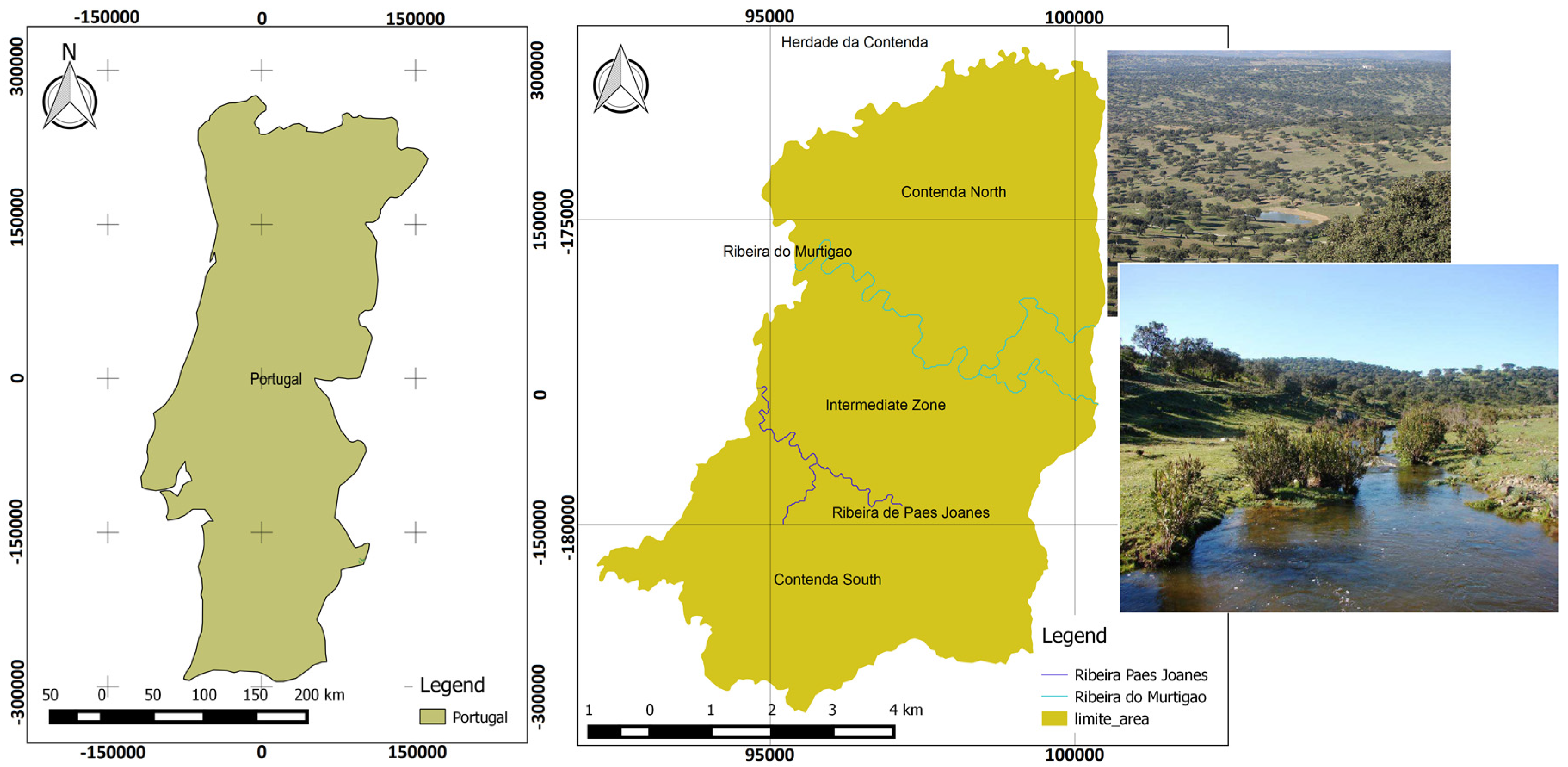
2. Study Case and Dataset

The Alentejo region (Portugal) shows climatic conditions reminiscent of those at the chosen SKA sites, and after preliminary RFI surveys, some locations showed excellent radio conditions with levels of interference comparable to SKA sites. From those surveys, HC was found to be the ideal site to install radio astronomy demonstrators. HC is a protected zone, National Hunt zone and Forestry Perimeter, located at the western part of the Serra Morena, in the municipality of Moura, Beja district, Portugal (Figure 1). The HC extends along 19 km of the Portuguese-Spanish border. With an area of 5270 ha, the Portuguese side is divided into three distinct areas: Contenda North (CN), Intermediate Zone (IZ) and Contenda South (CS) (Figure 1). In 1957, and from the request of the Moura municipality, the HC handed its management to the National Forest Authority (AFN—Autoridade Florestal Nacional). HC elevation values increase from 246 m to 543 m, with the south and southeast part having the highest elevation values. The slope values are lower closest to Ribeira do Murtigão (river), and the higher slope values are located in the oriental part. About 12% of the HC area is classified as Ibero-Mediterranean, with Quercus ilex predominance, and 88% as Sub-Mediterranean × Ibero-Mediterranean. The HC climate is humid and sub-humid. The annual average temperature is around 17.0 °C (maximum 24.3 °C and minimum 9.3 °C). The mean annual precipitation value is 729.5 mm with January and February presenting the highest values. During summer, the precipitation presents very low values. According to Oliveira [35], the typical soil classification is litossoils covering 98% of the HC area, and the Mediterranean soils covering the other 2% of the HC area. Litossoils are fragile soils with a thickness usually less than 10 cm and are very vulnerable to erosion phenomena.

In order to test the application, several maps were created with the methods incorporated in each menu. In the end, the GeoDecision tool was also tested with four of the maps created before. The factors were considered based on the available data for HC. Different spatial data were used in order to create the maps using the different menus, such as DEM generated from the flight performed in the area [10]; a geologic map (1/200,000 and different geologic information [35]; Land Cover Map 2007 shapefile data [36]; the economic values and vulnerability values were assigned based on the Municipal Defense Plan Against Forest Fire of Barrancos [37]; the slope map was derived from the DEM; a set of shapefiles with the burnt area information of 24 years (1990/2013) from the National Institute of Forest Conservation [34] were used; meteorological observations from a period of 27 years (1981–2008) were collected in the Alentejo weather station (38°38′59,28″N, 7°32′52,82″W); and the soil map (1/35,000) was based in PGFCFP soil map [34]. The DEM used has a spatial resolution of 10 m, and all of the data are in the European Terrestrial Reference System 1989 – Portugal Transversa de Mercator 2006 ETRS89 PTTM06 (EPSG: 3763) coordinate system.

3. Methodology

Based on the authors’ experience, the HCIEMS application was developed under a GIS open source application, specifically QGIS software, with the Python programming language [38,39,40]. The official QGIS file structure was followed, and several scripts, classes and functions were developed and implemented. Several libraries and Application Programming Interfaces (APIs) were used: Geospatial Data Abstraction Library (GDAL)/OGR Simple Feature Library, PyQt4 API, QGIS API, Numpy library and Python libraries, such as os, sys and glob [41,42,43,44,45]. Several classes were developed in order to incorporate the methods defined in the application (Figure 2). Each button and menu was developed with its own graphic interface composed of inputs, parameters and output fields. The input and output field allows one to access the file through a directory path. Besides the fields referred to, three standard buttons were added to each graphic interface: the OK, cancel and help buttons.

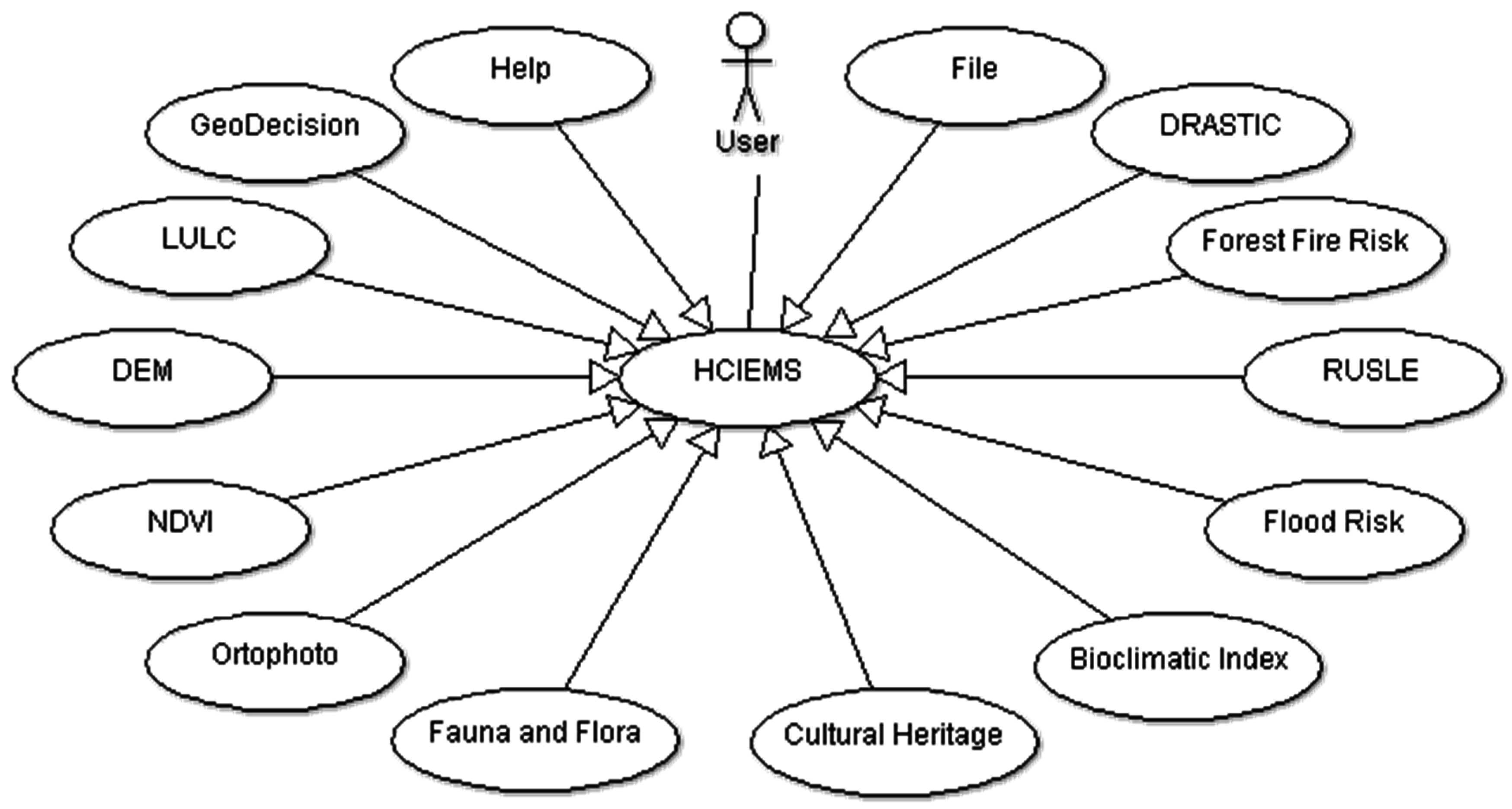
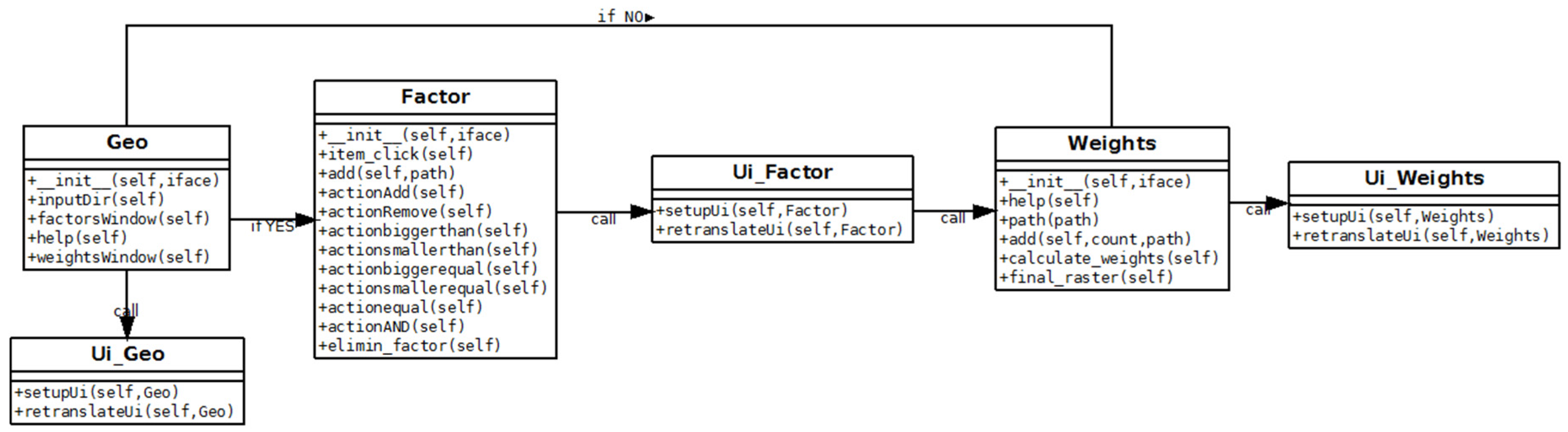
3.1. HCIEMS Graphic Interface

The first version of the HCIEMS application incorporated five buttons under a standard toolbar and twelve menus: file, DRASTIC (Depth to groundwater (D), Recharge (R), Aquifer media (A), Soil media (S), Topography (T), Impact of the vadose zone (I) and hydraulic Conductivity (C)), forest fire risk, Revised Universal Soil Loss Equation (RUSLE), bioclimatic index, heritage visualization, fauna and flora, orthophoto, NDVI, DEM, LULC and help [10]. The version described here is an improvement of the HCIEMS graphic interface with new incorporated methods, new functionalities—mainly in bioclimatic index and heritage visualization menus—and the creation of new menus: the flood risk menu and the decision making tool (GeoDecision). Figure 3 shows the HCIEMS user case diagram.

In order to improve the geographic information manipulation, a table of contents was added to the graphic interface window, which allows visualization and manipulation of different layers in the desktop area. Three connection options were added: show extent, remove layer and zoom to layer, allowing one to show the layer extension limits, to remove the layer from the area and to zoom into the layer extension in the desktop area, respectively. These actions are displayed with a mouse click on each layer. In order to improve these options, a new class was added, initializing the QgsLayerTreeViewMenuProvider Class Reference from QGIS API. This class was implemented to allow the QgsLayerTreeView instance to provide custom context menus (opened upon right-click). QgsLayerTreeView extends QTreeView and provides functionalities in order to work with a layer tree [42]. The QTreeView class belongs to the PyQt4 API and provides a model/view implementation of a tree view. This class implements a tree representation of items from a model, and it was used to provide standard hierarchical lists that were previously provided by the QListView class, but using the more flexible approach provided by Qt‘s model/view architecture [42]. Figure 4 presents the graphic interface with the improvement methods and menus.

3.1.1. DRASTIC Menu

The DRASTIC menu incorporates the DRASTIC index defined according to Aller et al. [46], and it is composed of seven factors disposed as buttons and dialog windows. The seven factors correspond to Depth to groundwater (D), Recharge (R), Aquifer media (A), Soil media (S), Topography (T), Impact of the vadose zone (I) and hydraulic Conductivity (C). In each of these factors, several inputs are required. DEM and the drainage network are required for the D parameter, which consists of two different methods: interpolating data points with the depth to groundwater values into a raster file or creating a Depth to groundwater (D) surface from DEM, where a surface is created through drainage network segments. The precipitation, overland flow, evapotranspiration data and also DEM are used as inputs in the R parameter following three distinct methods. The first method is the net recharge estimation according to a simplified water budget and based on $Recharge=precipitation-overland flow-evapotranspiration.$ The second method requires the availability of recharge rates expressed as a percentage of mean annual precipitation data (mm/year), assuming a constant recharge value for the entire study region. Finally, the third method uses DEM coupled with a regression model expressing precipitation as a function of altitude to calculate the spatial distribution of precipitation [47]. In order to obtain the A parameter, geological maps are used, and the ratings are assigned to the geologic material. As with the A parameter, the S parameter, based on soil maps, is obtained assigning the specific ratings. The I parameter is also obtained based on geological maps. The T parameter determination incorporates two methods, based either on the contour file or on DEM, in order to derive the slope and assign the ratings. Finally, the C parameter is obtained from hydraulic conductivity values, which are usually obtained from pumping tests or based on literature and may be introduced by the user in the attribute table of the geological vector file. The DRASTIC index corresponds to the final map, a result from the sum of the seven factor maps created before being multiplied by the corresponding weights as defined in Equation (1), according to Aller et al. [46]:

DRASTIC = D_R × D_W + R_R × R_W + A_R × A_W + S_R × S_W + T_R × T_W + I_R × I_W + C_R × C_W

(1)

where R and W (in subscript) correspond to the rating and weight for each factor, respectively. Some of these inputs are directly added (e.g., soil maps, geologic maps), and others are generated through this application (e.g., DEM, drainage network). Through the dialog windows, the user must define the parameters and obtain the factor maps, as well as the final DRASTIC index map. More information about this DRASTIC can be found in [40,47].

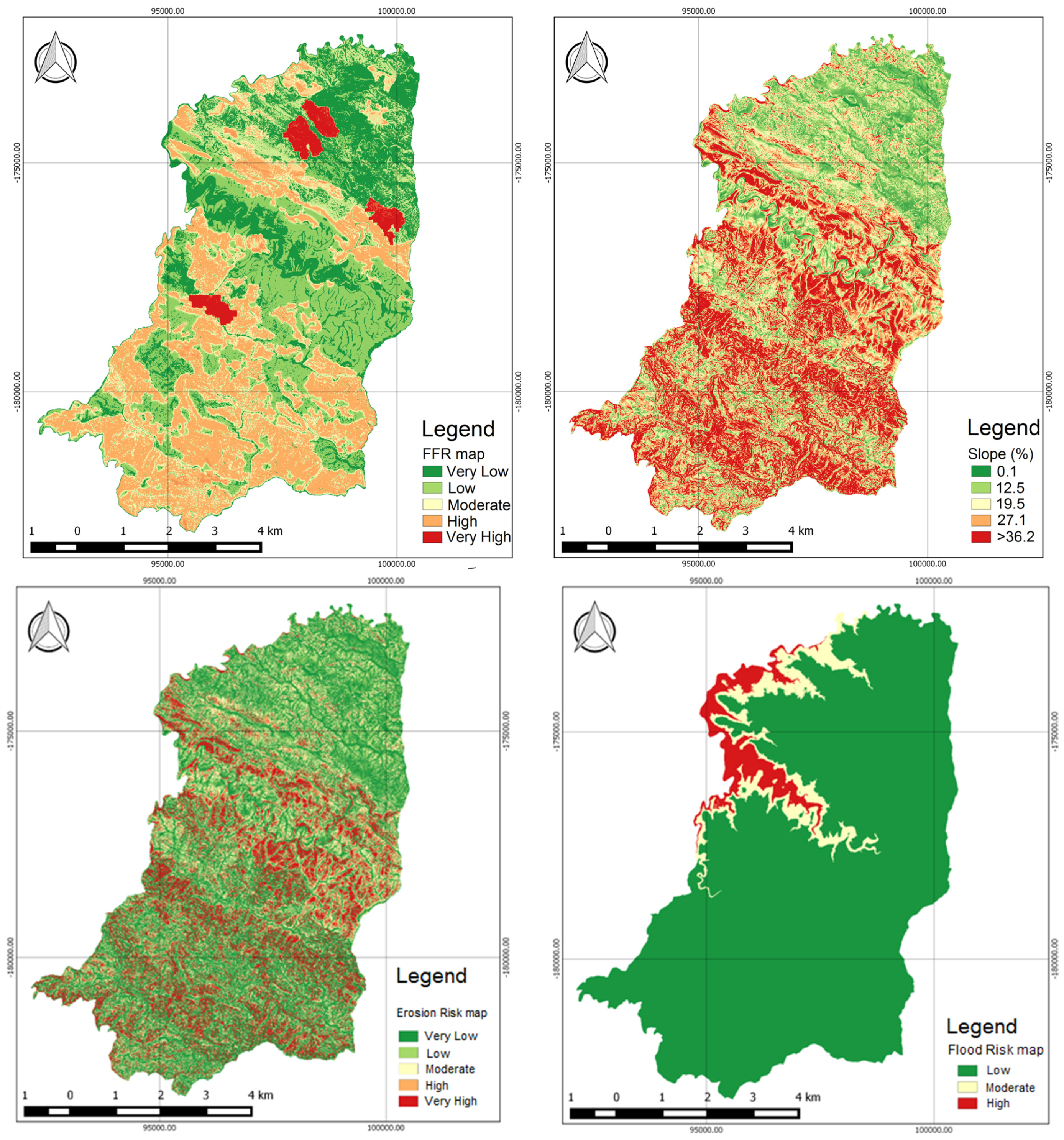
3.1.2. Forest Fire Risk Menu

The Forest Fire Risk (FFR) tool incorporates the forest fire risk assessment according to the rules published in the technical guide from the Portuguese Forest Authority [48], and it is composed of six buttons. Each one has a window with several options, such as menus, labels, edition windows, combo boxes and simple buttons, like OK, close and help, among others that help the user to access inputs and outputs directories. The hazard variables required in this application are the DEM to generate the slope map for the susceptibility map, the burned areas map for the probability map, the LULC map for susceptibility map and the economic values and vulnerability values of the land for each pixel. The hazard map is obtained from the multiplication of the probability and the susceptibility maps. The risk map is obtained from the multiplication of the hazard and the potential loss map. The potential loss map is obtained from the multiplication of the vulnerability and the economic value maps. Vulnerability values represent the damage level of an element at risk varying between 0 and 1, and economic values represent the price, in euros, of the land for each pixel. As in the previous menu, the DEM is generated in this application, and different methods for its generation are available. Each button allows on to create a map that will be used in the final hazard and risk map. More information about this menu can be founded in [10,38,39]. The interpretation of the FFR level is a crucial subject to mapping risk areas.

3.1.3. RUSLE Menu

The RUSLE menu allows for the estimation of the Revised Universal Soil Loss Equation (RUSLE), which corresponds to an estimation of the expected soil loss by water-caused erosion. The RUSLE method incorporates five erosion factors: rainfall-runoff erosivity factor (R), soil erodibility factor (K), topographic factor (LS), land cover factor (C) and practices factor (P). The estimation of the mean annual soil loss can be obtained using the following equation [49]:

A = R × K × LS × C × P

(2)

where A is the computed estimation of average annual soil loss (ton·km⁻²·year⁻¹), R is the erosivity factor calculated over 1 year, a measure of the erosive forces of rainfall-runoff (MJ·mmkm⁻²·h⁻¹·year⁻¹), K is the soil erodibility factor (ton·km²·h·km⁻²·MJ⁻¹·mm⁻¹), LS (unitless) is the combination of slope length (L) and slope steepness (S), C (unitless) is the land cover factor and P is the practices used for erosion control (unitless, ranging between 0 and 1). The R factor was incorporated based on Loureiro and Coutinho’s [50] approach, which estimates the RUSLE EI30 (the summation for each rainstorm of the kinetic energy (expressed in MJ/ha), multiplied by the greatest amount of rain in any 30 min period expressed in millimeters per hour [49]) index through a multiple linear regression with monthly EI30, monthly rainfall for days with ≥10.0 mm (rains 10) and monthly number of days with ≥10.0 mm (10 days). The monthly EI30 values are computed as the sum of EI30 for each erosive storm that occurs during the month and rains 10 and 10 days rainfall parameters are derived. The K factor was incorporated based on Wischmeier et al. [49]:

K = (2.1 × 10⁻⁴(12−OM) × M^1.14 + 3.25(s−2) + 2.5(p − 3))/100

(3)

where OM is the organic matter (%), s is the soil structure class, p is the permeability class and M is the aggregated variable derived from the granular soil texture: M = (%Msilt) × (%silt + %sand); and the modified silt (Msilt) is a percentage of grain size between 0.002 and 0.1 mm. If these data are not available, the menu incorporates the tables suggested for Portugal by Pimenta [51]. The LS factor proposed that the slope length and slope steepness can be used in a single index, which expresses the ratio of soil loss as shown in Equation (3) [52]:

LS = (X/22.1)^m (0.065 + 0.0456 × S + 0.0065 × S²)

(4)

where X is related to slope length (meters) and S corresponds to slope steepness (in percentage) and can be derived from a DEM. The m value varies from 0.2–0.5, depending on the slope percent: slope ≥5%, m = 0.5; slopes of 3.5%–4.5%, m = 0.4, slopes of 1–3, m = 0.3, slope <1% or uniform gradients, m = 0.2. In order to obtain the C factor, different approaches were employed: the image classification algorithm-based one is commonly used [53,54,55,56], as well as the Corine Land Cover (CLC) map [57,58]; and several tables were developed and published for the Portugal mainland [51]. The P factor is estimated using the method proposed by Kumar and Kushwaha [58], which is based on land cover/land use information. Considering the different type of land use, the P factors are assigned according to the values defined in the literature. In each of these erosion factors, several inputs are needed: meteorological data, soil map, DEM and land cover. Some of these inputs are directly added (e.g., soil maps, meteorological data), and others are generated through this application (e.g., DEM). This application also provides several interpolation methods. Finally, the RUSLE map combines the five factors previously created. More information about this menu can be found in [10]. The interpretation of the soil erosion level is a crucial subject to mapping risk areas regarding soil erosion prevention.

3.1.4. Flood Risk Menu

A new menu was created, the flood risk menu, which allows one to simulate the flood risk. This functionality was developed using the r.lake.coords algorithm from GRASS [59]. Based on a seed defined by the coordinates and the water level, the algorithm filled the lake in the specified point to the given level. Thereby, the user can simulate a flood in the study zone. This criterion can be useful as input in the decision making tool.

3.1.5. Bioclimatic Index Menu

According to PGFCFP [34], the bioclimatic indexes and parameters that should be considered were: continentality Index (Ic), termicity Index (It), compensated termicity Index (Itc), annual positive Temperature (Tp), annual negative Temperature (Tn), annual mean Precipitation (P), positive Precipitation (Pp) and the ombrothermic Index (Io). The indexes were performed according to PGFCFP [34];

Table 1. Bioclimatic indexes’ calculation.

Bioclimatic Index	Description
Continentality Index (Ic)	$Ic=\max (Tem{p}_{mmean12*})-\min (Tem{p}_{mmean12*})$
Termicity Index (It)	$It=(\frac{\sum Tem{p}_{mmean12*}}{12}+\min (Tem{p}_{mmean12*})+ Tem{p}_{min**})\times 10\mathrm{It}$
Compensated Termicity Index (Itc)	$if Ic<8: C_0=(8-Ic)\times 10;Itc=It- C_0$ $if 18>Ic\ge 8:Itc=It$ $if 21\ge Ic\ge 18: C_1=(Ic-18)\times 5;Itc=It+ C_1$ $if 28\ge Ic\ge 21: C_1=5\times (21-18); C_2=15\times (Ic-21);Itc=It+ C_1+ C_2$ $if 46\ge Ic\ge 28: C_1=15; C_2=105; C_3=25\times (Ic-28);Itc=It+ C_1+C_2+C_3$ $if 65\ge Ic>46: C_1=15; C_2=105; C_3=450; C_4=30(Ic-46);Itc=It+C_1+C_2+C_3+C_4$
Annual Positive Temperature (Tp)	$Tp=Tem{p}_{>0}\times 12$
Annual Negative Temperature (Tn)	$Tn= Tem{p}_{<0}\times 12$
Annual Mena Precipitation (P)	$P= \frac{\sum Prec***}{12}$
Positive Precipitation (Pp)	$Pp= {{\displaystyle \sum }}^{\text{}}Pre{c}_{Tempmmean12}****$
Ombrothermic Index (Io)	$Io= \frac{Pp}{Tp}\times 10$

* $Tem{p}_{mmean12}$: monthly mean of daily maximum temperatures (°C); ** $Tem{p}_{min}$: monthly mean of daily minimum temperatures (°C); *** $Prec$: total monthly precipitation (mm); **** $Pre{c}_{Tempmmean12}$: the corresponding precipitation value when the monthly mean of maximum temperatures are positive (mm).

presents the equations computed in order to obtain the bioclimatic indexes. Based on this information, the application was improved with a bioclimatic index menu, which allows one to read a text file with temperature and precipitation data and creates a Portable Document Format (PDF) file with the bioclimatic indexes calculated. The bioclimatic index menu is composed of five functions. In order to create a PDF file with the bioclimatic indexes’ description, the MATLAB-like plotting framework pyplot was used [60]. The figure is saved as PDF format through the savefig function. Through the subprocess command, the PDF is automatically opened.

3.1.6. Heritage Visualization Menu

According to Zaksek et al. [61], Sky View Factor (SVF) is a new relief visualization technique based on diffuse, rather than direct, illumination, corresponding to a portion of visible sky limited by relief, and it can be used to show relief characteristics. It can be helpful in archaeology, as it improves the recognition of small-scale features from high resolution DEMs. In this research, it was concluded that SVF is appropriate for general visualizations of heritage, giving a much better impression of the relative elevation of each point. Stular et al. [62] suggested several visualization techniques of high resolution DEMs for archaeological features’ visual detection and concluded that when archaeologists have to choose a single method, SVF method is endorsed, and the slope gradient is presented as an alternative method. Otherwise, according to the different terrain types, the interpreter must choose the appropriate technique. Stular et al. [62] showed that the most appropriate is the shift method or trend removal in combination with color cast on flat terrain, SVF on mixed terrain, slope gradient or trend removal on sloped terrain and SVF (blended with slope gradient) on rugged terrain. Following this, the heritage visualization menu was improved in order to perform the different techniques. Two different heritage features were identified in HC, namely a convent from the 17th century and an Iron Age hillfort. The heritage visualization menu is composed of visualization techniques that could be applied to different terrain types, particularly flat, rugged, mixed and sloped terrain. The user has the possibility to choose the method according to the land type case. Heritage visualization assessment through GIS functionalities can be used for guidance and support in projects that involve decision making about the land use. In fact, it is known that GIS tools are extremely helpful in the field of archaeology, helping to look for patterns in different layers of spatial data and survey sites and features, among others. The method was incorporated based on the SVF technique.

The rugged terrain and the mixed terrain implementation are identical. A graphic interface is composed of an input field (DEM); the parameter maximum search radius; the method: multi-scale or sectors; a field to multi-scale factor parameter; a field to number of sectors parameter; and six output fields were created. The rugged and mixed tools used the sky view factor algorithm from SAGA under two options: multi-scale and sectors [63]. Sky view factor algorithm from SAGA is based on the SVF calculation proposed by Hantzschel [64] and based on Dozier and Frew [65]. The analytical hillshading surface is also generated in order to overlap the two created layers (with 50% of transparency) and to combine them for a 3D visualization of SVF. For that, the analytical hillshading algorithm from SAGA was used [63]. The transparency was performed through the set Opacity function of QgsRaster Layer.

The sloped terrain functionality is composed of an input field (DEM); three filter options: Gaussian Filter, Laplacian Filter and Resampling Filter; one output for each filter; and a final slope gradient output. The method creates a slope map through the slopeaspectcurvature algorithm from SAGA, which allows one to calculate the local morphometric terrain parameters slope, aspect and, if supported by the chosen method, also the curvature. Concerning the Gaussian Filter, the gaussianfilter algorithm from SAGA was incorporated. The parameters standard deviation and search radius were implemented as input fields. Furthermore, a search mode field with two options (square and circle) was incorporated. For the other methods, the procedure is identically: the laplacianfilter and resampling algorithms from SAGA were used [63]. In the case of Gaussian Filter, the result is obtained from the subtraction of the filtered data by the DEM through the rastercalculator algorithm from SAGA. In the case of the Resampling Filter, the procedure implemented is based on first cell size resampling with the desired resolution as the multiple of an input scale factor (up-scaling), using the nearest neighbor interpolation method, and the second procedure is the down-scaling to the original cell size using the B-spline interpolation method [63]. The resulting filter is subtracted from the original DEM, and the final result is obtained.

The flat terrain techniques combine the different filters applied to a slope terrain with the analytical hillshading data overlap. This procedure follows the same implementation steps as described in the slope terrain functionality.

3.1.7. Fauna and Flora Menu

A fauna and flora menu was created to incorporate the available data records on carnivore presence and the location of latrines of rabbits, for summer and winter. This menu was improved to create an interpolation surface based on the number of records of the carnivore or latrines occurrence, and a new functionality was added to the fauna and flora menu. It is composed of an input field to the records, an input field to define the mask in order to restrict to the area, two spin boxes to define the grid cell size (in meters), another spin box to define the interpolation surface cell size and an output field to save the interpolation surface. A grid with the cell size defined by the user is created through the vectorgrid algorithm from the QGIS library Processing Toolbox. The number of records existing in each cell is recorded through countpointsinpolygon, an algorithm from QGIS, and assigned to the grid centroids, also obtained through Polygon centroids, an algorithm from SAGA. In order to perform the assignment referred, the counting shapefile was rasterized through the rasterize algorithm from the gdalogr library, and the values were assigned through the addgridvaluestopoints algorithm from SAGA. The centroids with no count or NULL are selected and interpolated through the v.surf.idw algorithm from the GRASS library. This process can be performed for any type of habitat record in shapefile format.

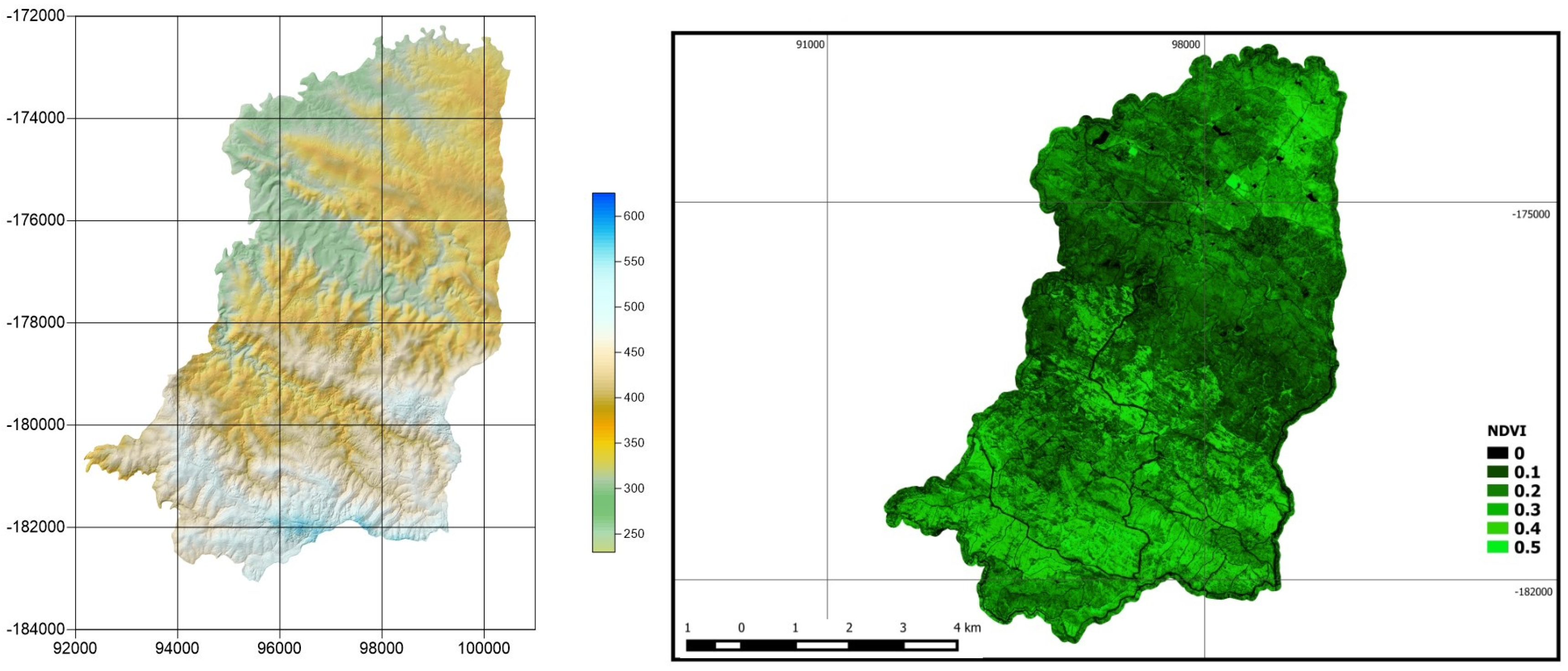
3.1.8. Orthophoto, DEM, LULC and NDVI Menus

Other types of information were incorporated in the application: orthophoto, DEM, LULC and NDVI. In order to obtain the DEM, a flight was performed with an aerial camera ZI-DMC, at a flying height of 2300 m, which resulted in an average pixel resolution of 20 cm on the ground. A total of 95 photos were collected, with a forward overlap of 60%, in 5 strips, with 30% side overlap. The camera is equipped with direct georeferencing equipment, based on the Global Positioning System (GPS) and an inertial navigation system. Each camera projection center was provided with an estimated positional accuracy of 5–10 cm. This allows for the photogrammetric mapping from these images without the need of ground control points for image orientation. The images were processed in Agisoft Photoscan. In this software, the image orientation was achieved by a bundle adjustment, based on conjugate points extracted automatically on the image overlaps and keeping the camera projection centers fixed. An initial sparse 3D point cloud was generated in the bundle adjustment process, which then was densified, in order to generate a 3D model with great detail of the terrain surface. A DEM in the form of a regular grid was then generated, with a 1-m grid spacing. The following step was the orthorectification of all of the individual photos, using the Digital Surface Model (DSM), which resulted in a rigorous georeferencing of all images. Finally, a continuous mosaic of all photos was done, with a resolution of 20 cm, resulting in a very large image, in Geotiff format. This was done for the RGB and NIR bands, each one having approximately 2 gigabytes. Overviews were created for these mosaics to allow for fast manipulation in a GIS [10].

The NDVI assumes values between −1 and +1 and is computed as NDVI = [(ρNIR-ρRed)/(ρNIR + ρRed)], where ρNIR and ρRed are respectively the near-infrared reflectance and red reflectance [66]. In this work, the NDVI map was computed using the red and NIR bands of the mosaic. The LULC map was computed using a supervised classification algorithm (maximum likelihood) with high accuracy (overall accuracy >99% and Kappa >0.99). The user can open just to visualize the data or can use it as inputs in the other tools developed. Figure 5 presents the DEM and NDVI maps. More information about these menus can be found in [10].

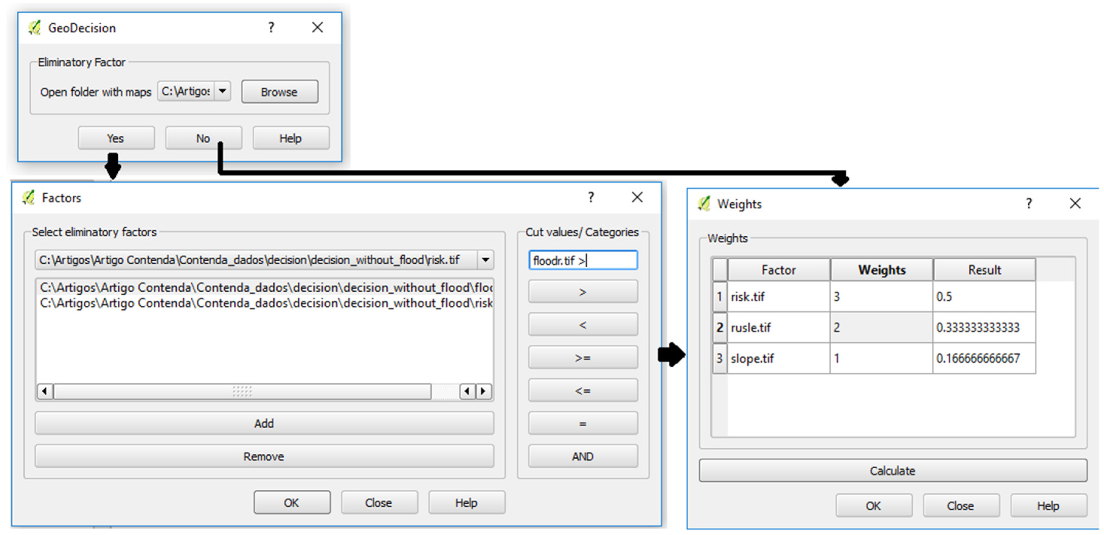
3.1.9. Decision Making Tool

The major improvement in the HCIEMS was the development of a decision making tool, GeoDecision. Figure 6 presents the GeoDecision class diagram.

The GeoDecision allowed the criteria assignment based on raster files in order to help in the selection of the most appropriate sites for the installation of the radio astronomy demonstrator. This application requires a directory with the raster files involved in the decision model. This connection was developed in the Geo class, through the inputDir function. Eliminatory factors should be firstly identified through the yes or no options presented with two buttons. If yes, the factorsWindow function from the Geo class is called, and the Factor class is imported. A new graphic interface is called with a combo box filled with the raster existent in the folder. The decision maker must select which ones have eliminatory values, through the add button. The raster files are listed in the table, and an editable expression appears in line edit. This clicked action is performed through the item_click function. In this section, the most used operators (>, <, ≥, ≤, ==, AND) are available to define the eliminatory values expression (Figure 6). Several functions were created in order to assign the operators. When the eliminatory values are defined, an OK button allows one to restrict each raster to the valid values, assigning “0” to eliminatory values through the elimin_factor function. In this function, each condition is implemented through the rastercalculator algorithm from SAGA, and finally, the resulting raster is multiplied by the original raster and is normalized to a scale from 0–100% through the gridnormalisation algorithm from SAGA. Next, the Weights class is called. A new graphic interface opens with the raster files and the weights for each one. By default, the weight values are defined as “1” to all raster and are shown in a table defined by QTableWidget from Qt API. The user can change the weight values and create different scenarios. The calculate button allows one to update the weight values, and calculate_weights is called. The weighting method incorporated in the application is performed as the division of the weight assigned by the sum of all weight values. The Final_raster function is then called and multiplies the calculated value for the previous raster.

If the no button is chosen, it is assumed that there were no eliminatory factors, so the original raster is normalized, and the weight assignment window is opened. This process is performed when the Weights class is called. The procedure is identically to the referred above, so the values are calculated based on weights and through the final_raster function. Figure 7 presents the graphic interface of GeoDecision.

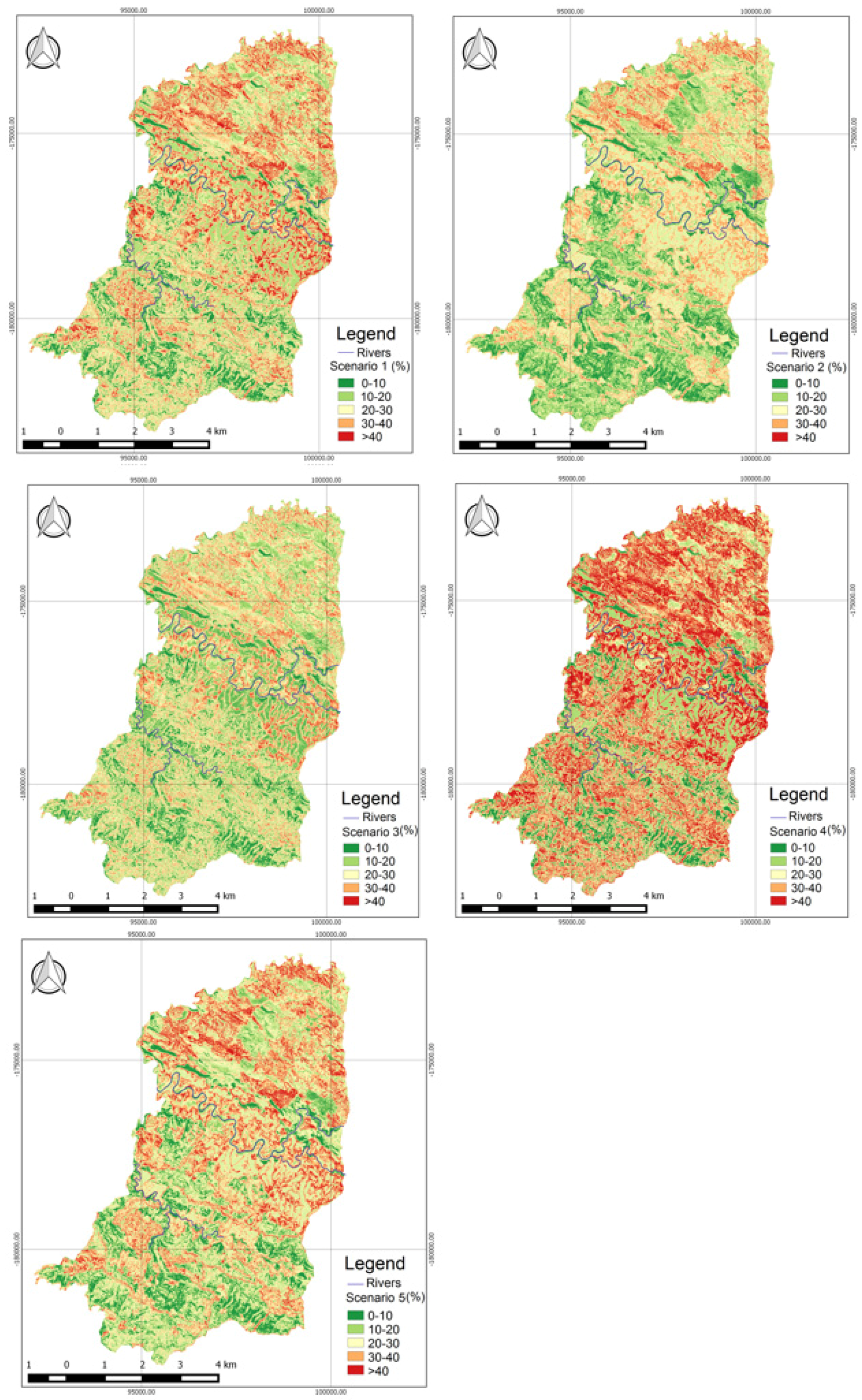
3.2. Demonstrator Multi-Criteria

The sites’ selection for the installation of the radio astronomy demonstrator implies three steps regarding the infrastructure: (i) safety; (ii) environmental impacts; and (iii) infrastructure access. The GeoDecision tool allows for the selection of the maps with the factors involved in the selection criteria, filtering out the information necessary to assess the sites of interest, so only four risk maps were used from all of the maps regarding the safety of the infrastructure. Although other criteria should be evaluated before the final decision, such as population density, road network and other human activities, the most important criteria regarding the infrastructure installation and the available data are based on the fire risk, the soil erosion level, the flood risk and the slope values. Since the area is a protected zone and a forest zone, fire risk and erosion risk are the most important criteria to be considered. If the installation is near the Ribeira do Murtigão, the flood risk is also relevant. The higher slope zones are excluded, since the installation must be in flat terrain, although with surrounding elevations around to protect from radio interference from the horizon. Figure 8 presents the multi-criteria factors considered in this work. In the HC area, only four maps were used in decision making due to the data availability. More data are required to create the other maps (DRASTIC, RUSLE, among others) and incorporate in the decision tool. Unfortunately, this was not possible in the HC area. However, the functionalities incorporated could be very useful in other areas’ studies, and the results can be used in the GeoDecision tool. For instance, the DRASTIC evaluation is very important in protected areas, so it is available in the tool, and the result can be easily used in the decision tool.

Based on the Report and Recommendation of the SKA Site Advisory Committee (SSAC) [67], climate, solar radiation, wildlife, land use restrictions, wildfires, seismic hazards and others were the environmental aspects considered in the sites’ evaluation and were considered accordingly in the site selection. In a second step, the environmental impacts of the infrastructure in the HC zone are also crucial to the installation. Factors, such as habitat consideration (fauna and flora, latrines and carnivores), cynegetic aspects, groundwater vulnerability and the cost strategies, must be considered. The final step is related to the analysis of the infrastructure access. Although the demonstrators will be operated remotely, some maintenance will be needed. According to PGFCFP [34], access roads were defined in HC. Other factors, such as tropospheric turbulence, political, socioeconomic and financial, legal and security factors, must be also considered [67].

The maps resulting from GeoDecision tool are classified from 0%–100%, where the higher the percentage, the more adequate is the site for the radio astronomy demonstrator installation. In order to interpret the maps generated, a symbology with five classes manually defined was applied: inadequate (0%–10%), not adequate (10%–20%), moderate adequacy (20%–30%), adequate (30%–40%) and very adequate (>40%). This classification can be adapted to an existing method in QGIS, and the classes’ values can be defined accordingly.

4. Results

A thorough study was performed in HC, the site chosen to install the radio astronomy demonstrators. Based on available data and based on the information of PGFCFP [34], several maps were created in order to obtain a final map through the decision making tool. In order to create the flood risk map, Ribeira do Murtigão was taken as the reference (0 m), and it was considered to be 300 m from the river. In the decision making tool, the flood risk map was reclassified as a zero value in zones with no risk of flood (<0 m), one (0–20 m) and two (>20 m) in the zones with more risk. The hazard map and the FFR map were created through the Land Use Map 2007 shapefile data, and the economic values and vulnerability values were assigned. The slope map was derived from the DEM, and the probability map was created from the set of shapefiles with the burnt area information. Based on this information, HC only has records for the years 2001 and 2002. The soil erosion risk map was created based on the meteorological data (R factor), and a value of 0.39 (litossoils) was assigned for the total HC area; DEM was used to obtain the LS factor, and Land Use Map 2007 was used to create the C and P factors. The slope map was created from the DEM. Figure 9 presents the maps involved in the decision making tool. The remaining maps, such as DRASTIC, RUSLE or other maps, were not taken into account in the HC area, because at this moment, the SKA project installation does not have all of the data required to integrate it in the final decision tool available. When this information become available, the procedure will be exactly the same as was explained in the previous sections. However, the application has already incorporated the functionalities to be tested in other protected areas.

The decision making tool was tested with the conditions referred to, and the more appropriate zones were predicted. Several scenarios were created in order to test the GeoDecision tool. In order to choose the most adequate weights, the weights were assigned based on field observations. Several field campaigns were performed in HC. Although flood risk was part of the decision rule, it was used only in one scenario. Figure 10 and

Table 2. Scenarios’ weights. FFR, Forest Fire Risk.

Weights	FFR	Erosion Risk	Slope	Flood Risk
Scenario 1	1	1	1	-
Scenario 2	3	2	1	-
Scenario 3	1	3	2	-
Scenario 4	2	1	3	-
Scenario 5	1	1	1	1

present the scenarios considering different weights. For most of the sites, any factor always has a small risk. As a natural consequence, no site was found with 100% adequacy.

5. Discussion

Regarding the slope map (Figure 9), 38.4% of the HC area was classified with very low or low values especially in the CN. The higher slope values were located in the CS with 19.2%. These areas can be related with the high and very high FFR zones, located in the CS, which cover 2.2% and 32.6%, respectively (Figure 9). Therefore, zones with high slope values were related with high FFR. Fifty six percent of the HC area was classified with low and very low FFR. These zones were located in the CN and in the IZ near Ribeira do Murtigão. This study showed that only years 2001 and 2002 presented fire occurrences. Therefore, these areas were classified with very high FFR. The results obtained reflect the data provided in PGFCFP [34], where the CS presents a higher FFR than the CN. Regarding the erosion risk map (Figure 9), CS and IZ present the majority of high erosion risk (13.9%). The CN presented a low erosion level perhaps due to the Quercus ilex plantation, which covers the total extension of the north area. Approximately 10% of the HC area was classified with high and very high erosion risk combined with high slope values, according to the RUSLE method. Most of these areas were located in the CS. Therefore, high slope values were related with a high erosion risk level. The low erosion risk level covered the CN and was detected in 54.2% of the total area.

From the different scenarios tested, it was concluded that the most adequate sites to install the demonstrator infrastructure were located in the CN, where the low percentage of risk prevailed. In Scenario 1, the weights were equally distributed by FFR, erosion and slope factors, and 9.88 km² of the area corresponded to the most adequate zones for the installation, which covered approximately 20% of the HC. These zones were situated in CN and IZ. In Scenario 2, a higher risk to FFR was assigned, with decreasing risks for erosion and slope factors. Considering these, 4.89 km² of the area were related to zones with more adequacies, and as in the previous scenario, the majority of these zones were located in the CN. The zones with higher FFR were automatically removed. In Scenario 3, erosion risk was assigned with a higher weight, with decreasing weight for the slope and FFR factors. In this scenario, 5.35 km² of the area were considered as the more adequate zones and covered the CN and the east part of HC. If the slope factor was considered as the most important and influential, decreasing FFR and erosion, 20.88 km² of HC had the perfect conditions, which was 40% of the total area. These zones were related with the low slope values zones. The CN was mostly classified as adequate. In the last scenario, the flood simulation was taken into account, and the weights were equally distributed. The result shows that 9.78 km² of HC satisfy the conditions. As with the previous scenarios, most of the zones were located in the CN. The flood risk could be improved with a more complex model in order to improve the decision final map and evaluate the flood risk. For instance, a hydraulic model could be incorporated. The literature reports that several works already integrate flood risk and hydraulic models in a GIS environment. For instance, Abdalla et al. [68] presents a GIS-supported three-dimensional fuzzy risk assessment approach for flood risk assessment. This is based on the development of a fuzzy-set risk model, 3D GIS mapping, and a hydro-statistical simulation. This method was applied to a section of the Red River in Southern Manitoba, Canada. Rahmati et al. [69] aimed to assess the efficiency of the analytical hierarchical process to identify potential flood hazard zones by comparing with the results of a hydraulic model. Initially, four parameters, like distance to river, land use, elevation and land slope, were used in some parts of the Yasooj River, Iran. This set of criteria was integrated through a weighted linear combination method using GIS proprietary software to generate a flood hazard prediction map. In order to validate the application, only a few scenarios were considered. However, according to these, the CN and, eventually, the IZ, next to the river, were the most adequate zones for the radio astronomy demonstrator infrastructure. Other factors will be taken into account for the final decision, such as the DRASTIC map, fauna and flora influence, heritage and others. However, HCIEMS returned a map considering several factors with assigned weights. In addition, this application is free and open source, enabling the combination of several scenarios assigning different weights.

6. Conclusions

The developed application, HCIEMS, allows for the monitoring and assessment of several environmental factors. Through its enhanced graphical interface, besides the standard buttons and functionalities, this application incorporates a decision making tool created in order to find the more appropriate sites to install radio astronomy demonstrators and develop a roadmap for future radio astronomy experiments in an international context. In this work, five examples were described. In the future, new and improved tools, new methods and functionalities and mitigation strategies will be incorporated, to better control the risks and minimize the potential impact of several phenomena (natural or human) and reduce the loss of resources. This new approach will involve mitigation measures, supportive infrastructure and an effective response. Although other criteria should be evaluated before any final decision, such as population density, road network, groundwater vulnerability, fauna and flora influence, heritage and human activities, in the present study, the most important criteria regarding the infrastructure installation were based on the available data, i.e., the fire risk, the soil erosion level, the flood risk and the slope values. Other factors should be evaluated in a second phase to minimize the environmental impacts, such as the study of local biodiversity factors. Anthropogenic factors must be also taken into account. The final decision for the installation of radio astronomy experiments will be based on all of the criteria already obtained and the data and improved methods that will be implemented, followed by an RFI survey to precisely describe the sites’ local radio environment.

This tool, with its unique integrated functionalities, can become a fundamental tool to guide decision making and the site-selection process of potential radio astronomy sites, in particular those requiring large territorial analysis that many times have information gaps or require specific approaches to handle the available information. Mega projects, like the SKA and most of its precursors or pathfinders, will be built in phases, expanding the antenna locations through several countries that certainly may benefit from an approach tested in a suitable territory emulator. In particular, the SKA African Partner countries may benefit from an integrated, centralized application that promotes and sources synergies between radio astronomy, GIS and space and Earth sciences as a first decision making step. The main focus of this research is the application created. The application incorporates several functionalities in order to create different maps. These maps can be (or not) included in the GeoDecision tool. Furthermore, the HCIEMS allows for improvement, modifications and adaptations to other protected/natural areas and can incorporate or target other functionalities. HCIEMS is open source and free; it can be easily incorporated with other spatial information (available at http://www.fc.up.pt/pessoas/liaduarte/HCIEMS.rar), and the details can be obtained upon request.

References

1. Schilizzi, R.T.; Dewdney, P.E.F.; Lazio, T.J. The square kilometre array. In Proceedings of the Ground-based and Airborne Telescopes II: 70121I, SPIE 7012, Marseille, France, 23 June 2008.
2. Umar, R.; Abidin, Z.Z.; Ibrahim, Z.A. The importance of site selection for radio astronomy. J. Phys. 2014, 539, 012009. [Google Scholar] [CrossRef]
3. Peng, B.; Sun, J.M.; Zhang, H.I.; Piao, T.Y.; Li, J.Q.; Lei, L.; Luo, T.; Li, D.H.; Zheng, Y.J.; Nan, R. RFI test observations at a candidate SKA site in China. Exp. Astron. 2004, 17, 423–430. [Google Scholar] [CrossRef]
4. SKA. SKA Telescope Square Kilometre Array. Exploring the Universe with the World’s Largest Radio Telescope. 2016. Available online: https://www.skatelescope.org/ (accessed on 20 April 2016).
5. Umar, R.; Abidin, Z.Z.; Ibrahim, Z.A. The importance of Radio Quiet Zone (RQZ) for radio astronomy. AIP Conf. Proc. 2013, 1528, 32. [Google Scholar]
6. Zhu, B.; Nie, Y.; Nan, R.; Peng, B. The FAST/SKA site selection in Guizhou province. Astrophys. Space Sci. 2001, 278, 213–218. [Google Scholar] [CrossRef]
7. Aksaler, N.; Yerli, S.K.; Erdogan, M.A.; Kaba, K.; Ak, T.; Aslan, Z.; Bakis, V.; Demircan, O.; Evren, S.; Keskin, V.; et al. Astronomical site selection for Turkey using GIS techniques. Exp. Astron. 2015, 39, 547–566. [Google Scholar] [CrossRef]
8. Rughooputh, S.D.D.V.; Oodit, S.; Persand, S.; Golap, K.; Somanah, R. A new tool for handling astronomical images. Astrophys. Space Sci. 2000, 273, 245–256. [Google Scholar] [CrossRef]
9. Barbosa, D.; Aguiar, R.; Barraca, J.P.; van Ardenne, A.; Boonstra, A.J.; Verdes-Montenegro, L.; Santander-Vela, J. A Sustainable approach to large ICT Science based infrastructures; the case for Radio Astronomy. In Proceedings of the IEEE International Energy Conference—ENERGYCON, Dubrovnik, Croatia, 14 May 2014.
10. Teodoro, A.; Duarte, L.; Sillero, N.; Gonçalves, J.A.; Fonte, J.; Gonçalves-Seco, L.; Pinheiro da Luz, L.M.; dos Santos Beja, L.M.R. An integrated and open source GIS environmental management system for a protected area in the south of Portugal. In Proceedings of the SPIE 9644, Earth Resources and Environmental Remote Sensing/GIS Applications VI, Toulouse, France, 24 September 2015.
11. Van Ardenne, A.; Bregman, J.D.; van Cappellen, W.; Kant, G.W.; bij de Vaate, J.G. Extending the field of view with Phased Array Techniques. Proc. IEEE 2009, 97, 1531–1542. [Google Scholar] [CrossRef]
12. Faulkner, A.; Alexandre, P.; van Ardenne, A.; Bolton, R.; Bregman, J.; van Es, A.; Jones, M.; Kant, D.; Montebugnoli, S.; Picard, P.; et al. SKA Memo 122: Aperture Arrays for the SKA: the SKADS white Paper. 2010. Available online: https://www.skatelescope.org/public/2011-06-28_Signal_Transport_and_Networks_CoDR/CoDR_Applicabledocuments/AppDoc11_122_Memo_Faulkner.pdf (accessed on 9 October 2016).
13. Torchinsky, S.A.; van Ardenne, A.; den Brink-Havinga, T.; van Es, A.J.J.; Faulkner, A.J. Wide field astronomy & technology for the square kilometre array. In Proceedings of the SKADS Conference, Limelette, Project “SKADS” Contract No. 011938, and Marie Curie Actions Contract No. 46095, Limelette, Belgium, 4–6 November 2009.
14. Torchinsky, S.A.; Broderick, J.W.; Gunst, A.; Faulkner, A.J.; van Cappellen, W. SKA Aperture Array Mid Frequency Science Requirements, SKA Mid Frequency Aperture Array System Requirements Review; SKA-TEL-MFAA-0200009; ASTRON: Dwingeloo, The Netherlands, 2016. [Google Scholar]
15. Boonstra, A.J.; Millenaar, R. AAVP Spectrum Monitoring, Herdade Ferradura and Contenda Forrest Surveys, Portugal; Tech. Rep., ASTRON-RP-391; ASTRON: Dwingeloo, The Netherlands, 2010. [Google Scholar]
16. Ambrosini, R.; Beresford, R.; Boonstra, A.-J.; Ellingson, S.; Tapping, K. RFI Measurement Protocol for Candidate SKA Sites; Ellingson, S., Ed.; SKA Memo 37, Internal Report from the SKA International Working Group on RFI Measurements; SKA: Cheshire, UK, 2003. [Google Scholar]
17. ANACOM. National Frequency Allocation Plan, 2008; ANACOM: Lisbon, Portugal, 2009. [Google Scholar]
18. Chi Aye, Z.; Jaboyedoff, M.; Derron, M.; van Westen, C.J. 2015 Prototype of a Web-based Participative Decision Support Platform in Natural Hazards and Risk Management. ISPRS Int. J. Geo-Inf. 2015, 4, 1201–1224. [Google Scholar]
19. Puniway, N.; Canale, L.; Haws, M.; Potemra, J.; Lepczyk, C.; Gray, S. Development of a GIS-based tool for aquaculture siting. ISPRS Int. J. Geo-Inf. 2014, 3, 800–816. [Google Scholar] [CrossRef]
20. Feizizadeh, B.; Blaschkea, T. An uncertainty and sensitivity analysis approach for GIS-based multicriteria landslide susceptibility mapping. Int. J. Geogr. Inf. Sci. 2014, 28, 610–638. [Google Scholar] [CrossRef] [PubMed]
21. Ullah, K.M.; Mansourian, A. Evaluation of land suitability for urban land-use planning: Case study dhaka city. Trans. GIS 2016, 20, 20–37. [Google Scholar]
22. Aydi, A.; Abichou, T.; Nasr, I.H.; Louati, M.; Zairi, M. Assessment of land suitability for olive mill wastewater disposal site selection by integrating fuzzy logic, AHP, and WLC in a GIS. Environ. Monit. Assess. 2016, 188, 1–13. [Google Scholar] [CrossRef] [PubMed]
23. Berry, R.; Higgs, G. Gauging levels of public acceptance of the use of visualisation tools in promoting public participation; a case study of wind farm planning in South Wales, UK. J. Environ. Plan. Manag. 2012, 55, 229–251. [Google Scholar] [CrossRef]
24. Higgs, G.; Berry, R.; Kidner, D.; Langford, M. Using IT approaches to promote public participation in renewable energy planning: Prospects and challenges. Land Use Policy 2008, 25, 596–607. [Google Scholar] [CrossRef]
25. Jahani, A.; Feghhi, J.; Makhdoum, M.F.; Omid, M. Optimized forest degradation model (OFDM): An environmental decision support system for environmental impact assessment using an artificial neural network. J. Environ. Plan. Manag. 2016, 59, 222–244. [Google Scholar] [CrossRef]
26. Motlagh, Z.K.; Sayadi, M.H. Siting MSW landfills using MCE methodology in GIS environment (Case study: Birjand plain, Iran). Waste Manag. 2015, 46, 322–337. [Google Scholar] [CrossRef] [PubMed]
27. Qaddah, A.A.; Abdelwahed, M.F. GIS-based site suitability modelling for seismic stations: Case study of the northern Rahat volcanic field, Saudi Arabia. Comput. Geosci. 2015, 83, 193–208. [Google Scholar] [CrossRef]
28. Bricker, S.B.; Getchis, T.L.; Chadwick, C.B.; Rosa, C.M.; Rose, J.M. Integration of ecosystem-based models into an existing interactive web-based tool for improved aquaculture decision-making. Aquaculture 2016, 453, 135–146. [Google Scholar] [CrossRef]
29. Yang, Y.-C.E.; Lin, Y.-F.F. A new GIScience application for visualized natural resources. Trans. GIS 2011, 15, 109–124. [Google Scholar] [CrossRef]
30. Papadimitriou, F. Modelling landscape complexity for land use management in Rio de Janeiro, Brazil. Land Use Policy 2012, 29, 855–861. [Google Scholar] [CrossRef]
31. Papadimitriou, F. Artificial Intelligence in modelling the complexity of Mediterranean landscape transformations. Comput. Electron. Agric. 2012, 81, 87–96. [Google Scholar] [CrossRef]
32. Graser, A.; Straub, M.; Dragasching, M. Towards an open source analysis toolbox for street network comparison: Indicators, tools and results of a comparison of OSM and the official austrian reference graph. Trans. GIS 2014, 18, 510–526. [Google Scholar] [CrossRef]
33. QGIS. QGIS Project. 2016. Available online: http://www.qgis.org/ (accessed on 20 April 2016).
34. ICNF. Instituto da Conservação e da Defesa das Florestas. 2009. Available online: http://www.icnf.pt/portal (accessed on 22 April 2016).
35. Oliveira, J.T. Carta Geológica de Portugal Escala 1/200 000 Notícia Explicativa da Folha 8 Direcção Geral de Geologia e Minas; Serviços Geológicos de Portugal: Lisboa, Portugal, 1992. [Google Scholar]
36. dgTerritório. Direção-Geral do Território. 2015. Available online: http://www.dgterritorio.pt/cartografia_e_geodesia/cartografia/cartografia_tematica/carta_de_ocupacao_do_solo__cos_/cos__2007/ (accessed on 22 April 2016).
37. PMDFCI. Associação de Produtores da Floresta Alentejana. Plano Municipal da Defesa da Floresta Contra Incêndios de Barrancos. 2010. Available online: http://www.cm-barrancos.pt/smpc/PMDFCI.pdf (accessed on 22 April 2016).
38. Teodoro, A.C.; Duarte, L. Forest Fire risk maps: A GIS open source application—A case study in Norwest of Portugal. Int. J. Geogr. Inf. Sci. 2013, 27, 699–720. [Google Scholar] [CrossRef]
39. Duarte, L.; Teodoro, A.C. An easy, accurate and efficient procedure to create Forest Fire Risk Maps using Modeler (SEXTANTE plugin). J. For. Res. 2016, 27, 1–12. [Google Scholar] [CrossRef]
40. Duarte, L.; Teodoro, A.C.; Gonçalves, J.A.; Guerner Dias, A.J.; Espinha Marques, J. A dynamic map application for the assessment of groundwater vulnerability to pollution. Environ. Earth Sci. 2015, 74, 2315–2327. [Google Scholar] [CrossRef]
41. GDAL. Geospatial Data Abstraction Library. 2015. Available online: http://www.gdal.org/ (accessed on 30 March 2016).
42. PyQt4 API. PyQt Class Reference. 2015. Available online: http://pyqt.sourceforge.net/Docs/PyQt4/classes.html (accessed on 22 March 2016).
43. QGIS API. QGIS API Documentation. 2013. Available online: http://www.qgis.org/api/ (accessed on 22 March 2016).
44. Numpy API. Numpy Reference. 2015. Available online: http://docs.scipy.org/doc/numpy/reference/ (accessed on 22 March 2016).
45. Python. Python Programming Language. 2015. Available online: http://python.org/ (accessed on 22 March 2016).
46. Aller, L.; Lehr, J.H.; Petty, R.; Bennet, T. DRASTIC: A standardized system to evaluate groundwater pollution potential using hydrogeologic settings. Geol. Soc. India 1987, 29, 1–622. [Google Scholar]
47. Duarte, L.; Teodoro, A.C.; Gonçalves, J.A.; Dias, A.; Espinha Marques, J. Assessing groundwater vulnerability to pollution through the DRASTIC method. Lecture Notes Comput. Sci. 2014, 8582, 386–400. [Google Scholar]
48. DFCI. Plano Municipal da Defesa da Floresta Contra Incêndios. 2008. Available online: http://www.afn.min-agricultura.pt/portal/dudf/gtfs/planeamento-dfci-municipal/guia-metodologico-para-a-elaboracao-do-pmdfci (accessed on 20 April 2016).
49. Wischmeier, W.H.; Johnson, C.B.; Cross, B.V. A soil erodibility nomograph for farmland and construction sites. J. Soil Water Conserv. 1971, 26, 189–193. [Google Scholar]
50. Loureiro, N.S.; Coutinho, M.A. A new procedure to estimate the RUSLE EI30 index, based on monthly rainfall data and applied to the Algarve region, Portugal. J. Hydrol. 2001, 250, 12–18. [Google Scholar] [CrossRef]
51. Pimenta, M.T. Directrizes Para a Aplicação da Equação Universal de Perda dos Solos em SIG, Factor de Cultura C e Factor de Erodibilidade do Solo K; INAG/DSRH (Sistema Nacional de Informação dos Recursos Hídricos): Lisbon, Portugal, 1998. [Google Scholar]
52. Wischmeier, W.H.; Smith, D.D. Predicting Rainfall Erosion Losses: A Guide to Conservation Planning with Universal Soil Loss Equation (USLE); Agriculture Handbook, Department of Agriculture: Washington, DC, USA, 1978. [Google Scholar]
53. Arekhi, S.; Niazi, Y.; Kalteh, A.M. Soil erosion and sediment yield modelling using RS and GIS techniques: A case study, Iran. Arabian J. Geosci. 2012, 5, 285–296. [Google Scholar] [CrossRef]
54. Jiang, Z.; Su, S.; Jing, C.; Lin, S.; Fei, X.; Wu, J. Spatiotemporal dynamics of soil erosion risk for Anji County, China. Stoch. Environ. Res. Risk Assess. 2012, 26, 751–763. [Google Scholar] [CrossRef]
55. Xu, L.; Xu, X.; Meng, X. Risk assessment of soil erosion in different rainfall scenarios by RUSLE model coupled with Information Diffusion Model: A case study of Bohai Rim, China. Catena 2012, 100, 74–82. [Google Scholar] [CrossRef]
56. Alexakis, D.D.; Hadjimitsis, D.G.; Agapiou, A. Integrated use of remote sensing, GIS and precipitation data for the assessment of soil erosion rate in the catchment area of ”Yialias” in Ciprus. Atmos. Res. 2013, 131, 108–124. [Google Scholar] [CrossRef]
57. Fagnano, M.; Nazzareno, D.; Alberico, I.; Fiorentino, N. An overview of soil erosion modeling compatible with RUSLE approach. Rend. Lincei 2012, 23, 69–80. [Google Scholar] [CrossRef]
58. Kumar, S.; Kushwaha, S.P.S. Modelling soil erosion risk based on RUSLE-3D using GIS in a Shivalik sub-watershed. J. Earth Syst. Sci. 2013, 122, 389–398. [Google Scholar] [CrossRef]
59. GRASS GIS. The World’s Leading Free GIS Software. 2013. Available online: http://grass.osgeo.org/ (accessed on 22 March 2016).
60. Matplotlib. Matplotlib API. 2016. Available online: http://matplotlib.org/api/pyplot_api.html (accessed on 20 March 2016).
61. Zaksek, K.; Ostir, K.; Kokalj, Z. Sky-View Factor as a Relief Visualization Technique. Remote Sens. 2011, 3, 398–415. [Google Scholar] [CrossRef]
62. Stular, B.; Kokalj, Z.; Ostir, K.; Nuninger, L. Visualization of LiDAR-derived relief models for detection of archaeological features. J. Archaeol. Sci. 2012, 39, 3354–3360. [Google Scholar] [CrossRef]
63. SAGA. SAGA-GIS Module Library Documentation. 2016. Available online: http://www.saga-gis.org/saga_module_doc/2.1.3/ta_lighting_3.html (accessed on 22 March 2016).
64. Hantzschel, J.; Goldberg, V.; Bernhofer, C. GIS-based regionalisation of radiation, temperature and coupling measures in complex terrain for low mountain ranges. Meteorol. Appl. 2005, 12, 33–42. [Google Scholar] [CrossRef]
65. Dozier, J.; Frew, J. Rapid calculation of terrain parameters for radiation modeling from digital elevation data. IEEE Trans. Geosci. Remote Sens. 1990, 28, 963–969. [Google Scholar] [CrossRef]
66. Solano, R.; Didan, K.; Jacobson, A.; Huete, A. MODIS Vegetation Index User’s Guide (MOD13 Series); Vegetation Index and Phenology Lab, University of Arizona: Tucson, AZ, USA, 2010. [Google Scholar]
67. Moran, J.M.; Ananthakrishnan, S.; Baars, J.W.M.; Burnell, J.B.; Brouw, W.N.; Crocker, J.; Garvin, T.; Michalowski, S.; Seaquist, E.R.; Tindemans, P.; et al. Report and Recommendation of the SKA Site Advisory Committee (SSAC). 2012. Available online: http://www.skatelescope.org/uploaded/40391_120216_SSAC.Report_web.pdf (accessed on 9 October 2016).
68. Abdalla, R.; Elawad, Y.; Chen, Z.; Han, S.S.; Xia, R. A GIS-supported fuzzy-set approach for flood risk assessment. Can. Water Resour. J. 2014, 39, 3–14. [Google Scholar] [CrossRef]
69. Rahmati, O.; Zeinivand, H.; Besharat, M. Flood hazard zoning in Yasooj region, Iran, using GIS and multi-criteria decision analysis. Nat. Hazards Risk 2016, 7, 1000–1017. [Google Scholar] [CrossRef]
Figure 1. Study case: Herdade da Contenda (HC) region, Alentejo Portugal.
Ijgi 05 00209 g001
Figure 2. Herdade da Contenda Integrated Environmental Management System (HCIEMS) class diagram.
Ijgi 05 00209 g002
Figure 3. Herdade da Contenda Integrated Environmental Management System (HCIEMS) user case diagram. RUSLE, Revised Universal Soil Loss Equation and DRASTIC (Depth to groundwater (D), Recharge (R), Aquifer media (A), Soil media (S), Topography (T), Impact of the vadose zone (I) and hydraulic Conductivity (C)).
Ijgi 05 00209 g003
Figure 4. Herdade da Contenda Integrated Environmental Management System (HCIEMS) graphic interface.
Ijgi 05 00209 g004
Figure 5. DEM and NDVI maps incorporated in the application.
Ijgi 05 00209 g005
Figure 6. GeoDecision class diagram.
Ijgi 05 00209 g006
Figure 7. GeoDecision graphic interface (just for illustration purposes, the values presented are not the real ones).
Ijgi 05 00209 g007
Figure 8. Multi-criteria factors.
Ijgi 05 00209 g008
Figure 9. Maps involved in the decision making tool.
Ijgi 05 00209 g009
Figure 10. Scenarios tested through the GeoDecision tool.
Ijgi 05 00209 g010