Belgium through the Lens of Rail Travel Requests: Does Geography Still Matter?

Abstract

This paper uses on-line railway travel requests from the iRail schedule-finder application for assessing the suitability of that kind of big data for transportation planning and to examine the temporal and regional variations of the travel demand by train in Belgium. Travel requests are collected over a two-month period and consist of origin-destination flows between stations operated by the Belgian national railway company in 2016. The Louvain method is applied to detect communities of tightly-connected stations. Results show the influence of both the urban and network structures on the spatial organization of the clusters. We also further discuss the implications of the observed temporal and regional variations of these clusters for transportation travel demand and planning.

1. Introduction

Travel flows are commonly represented by graphs, wherein nodes are the origins, and destinations and edges are weighted by the intensity of the flows. Numerous applications have attempted to identify groups of nodes that share tight links, using community detection methods. Examples for home-to-work commuting include the Czech Republic [1], Ireland [2], Slovenia [3], the United Kingdom [4] and the city of Brussels [5] (in Belgium). All of these papers, however, rely on travel flows between administrative units, all transportation modes combined.

Relying on finer data, for instance divided by transport mode or at the public transport stops level, rather than administrative delineation, may provide further insights on travel behavior. Despite their limits and critics, information and communication technologies (ICT) are quite important for that purpose (see [6], for a review) and also offer many opportunities in human geography [7]. Their availability in streaming, that is the data being continuously updated over time, is especially attractive for transportation planning. In this paper, we take advantage of an original “big data” set: the travel requests by train in Belgium made through iRail, a schedule-finder website and application. The nodes represent the train stations, while the weight of a link $(i,j)$ is the number of travel requests between stations i and j.

The contributions of this paper are, therefore, two-fold. Our first objective is to assess the potential of datasets made of travel requests as a proxy for data on actual travel flows. Such information can be collected from nearly all public transport company websites or applications and has strong advantages in richness and availability compared to more traditional travel surveys (see Section 2). Here, this assessment relies on the case study of the travel by rail in Belgium. Our second objective is thus to provide a thorough analysis of the spatial structure of commuting by train in Belgium; such an in-depth study has never been presented in the existing literature (the closest example being [8]). The reason for this lack is data availability constraints, the privacy rules imposed by the Belgian national railway company preventing official data on railway transport use (such as ticket sales) to be disclosed. “Big data”, and more precisely the travel requests made on the schedule-finder website and application iRail between December 2015 and February 2016, are thus used as a proxy to overcome these limitations.

This second objective is tackled through the following research question: which of the urban and railway network structures has the strongest influence on the travel demand by train in Belgium? It is grounded in the economic geography literature: according to the gravity model of trade (see [9,10,11]) and, in particular, its applications to commuting (e.g., [12,13,14,15,16], and [17] for Belgium), the travel demand should be proportional to the weight of the origins and that of the destinations. Therefore, the first assumption tested for our case study is that the communities detected in the graph of the travel requests will be consistent with the urban structure of Belgium.

The gravity model of trade, however, also assumes that the interactions between two places are inversely proportional to the transport cost or distance between these places [9,18]. It is important here to note that the railway infrastructure is different from the travel demand network (see Figure 1). They share the same nodes (the train stations), but their links differ. For the former, a link represents the presence of a railway line between two stations, while for the latter, it is the number of passengers traveling between these stations. Although the railway network is very well developed in Belgium (see Section 3.1), its density and operating speed or frequencies vary throughout the country. The literature on transport geography provides various examples of how anisotropy in a transportation network (e.g., high-speed railways) affects the travel times and costs (e.g., [19,20,21,22,23]). Hence, our second hypothesis is that the physical railway network influences (through the travel distance) the shape and size of the communities detected in the travel demand network.

Our methodology consists of applying a community detection algorithm (the Louvain method; see [24]) to this travel-demand network, then comparing the spatial pattern of the communities with the urban and railway network structures, by cartographic representation and graph-theory indicators of centrality, following an approach similar to [25]. This procedure is conducted on eight subsets of the data, starting from all requests and afterwards examining temporal, linguistic and regional variations. The urban and home-to-work commuting structure of Belgium have been widely studied in previous research. See, e.g., [26], for the former, and [27,28], for the latter. We expect the spatial organization of commuting by train to be consistent with these studies, which would mean that travel requests accurately represent actual travel flows. If peculiarities emerge, the question will be to identify whether they are attributable to the mode studied (railway transport) or to the dataset itself.

To answer these objectives, the paper is organized as follows. Section 2 introduces the specificities of the dataset. The case study and the methodology used are detailed in Section 3. Results are presented in Section 4 and further discussed in Section 5. A conclusion is given in Section 6.

2. Travel Requests versus Travel Flows

Information on travel behavior is typically collected through households or workers’ travel surveys, such as the National Household Travel Survey in the U.S. [29] or, for our Belgian case study, the BELDAM (acronym for Belgian Daily Mobilities) survey [30] (see also [31] for an overview of national travel statistics in Europe). However, and although they can be of different types (trip-based or time use; see [32,33]), all of these surveys rely on relatively small samples and are only conducted (at best) on a per annum basis. Therefore, these surveys lack the richness in volume and velocity that ICT technologies provide.

To gather information about travel flows, the ideal situation is a transportation system where all passengers are required to present an electronic ticket to an automated gate or terminal both for entering and leaving the system (subways are the ground transportation systems fitting closest to this description). If so, exhaustive and real-time data on travel flows, in the form of an origin-destination (O/D) matrix, can be collected.

Nevertheless, the availability of these data remains limited. Examples published in the scientific literature appear limited to London [34], Beijing [35] and Shanghai [36], for various potential reasons. The most plausible are technical: not all transportation systems are equipped with automated ticket-control devices, and a passenger is often not required to scan his/her ticket or smart-card upon exit, thereby losing the destination component of the O/D matrix. The system described above also raises privacy issues, since it allows controlling all displacements of one individual.

Collecting travel requests made on an online schedule-finder website or application provides an elegant alternative to these shortcomings. They are, by nature, origin-destination information and pose no threat to privacy as long as the IP address of the device used to make the request is not stored. They also provide real-time data, although their exhaustiveness remains an open question. Finally, they possess the unique characteristic that a request can be made while planning for future travel; therefore providing insightful information for prospective transportation planning that no other dataset could deliver.

A travel requests’ dataset presents, however, its own methodological challenges. The main one is to assess whether it represents the actual travel flows. A request does not imply that a user actually did travel, and vice versa. Using our case study as an example, users can make the same request several times before traveling; friends of travelers may check on the arrival time of a train; and users who are used to traveling and know the timetable may not need to use iRail before their journey. Furthermore, the same information is also available on other websites, especially [37], the official website of the Belgian National Railway Company.

The question of whether the sample of online requests is representative of the actual travel demand is difficult to figure out. Indeed, one may argue that only users who do not already know the timetables will use the iRail service, therefore representing only non-routine behavior. However, the service also offers real-time updates of the possible delays, a service that could be used by commuters, as well as occasional travelers. Note that, in any case, this paper does not try to infer absolute numbers of travelers, but rather relies on the relative frequencies of routes among all travels.

3. Data and Methodology

3.1. Urban and Railway Structures of Belgium

Belgium is a densely-populated country (about 360 inhabitants per square kilometer, for a total of 11 million inhabitants in 2016) divided into three administrative regions: Flanders, Wallonia and the Brussels Capital Region (BCR), as shown on Figure 2a. Each of these regions has its own government and language (Dutch in Flanders, French in Wallonia, both in the BCR). Note that Wallonia is more extended and has hence a looser urban network, resulting in longer distances traveled.

Belgium has a clear urban hierarchy (Figure 2a) dominated by the metropolitan area of Brussels, centered on the BCR and located in the center of the country. The BCR accounts for 10% of the Belgian population as of 2016 [38] (18% for Urban Region of Brussels as defined by [26]) and attracts around 350,000 commuters per day [28,39]. Note that although the metropolitan area of Brussels is the largest one in Belgium and includes some neighboring cities, the city of Leuven stays out of its influence.

All of these urban areas are connected by major railroads (Figure 2b). In 1835, the first railway of the European continent was built in Belgium between Mechelen and Brussels. Many private companies then built their own railways, and the maximal extension of the Belgian network exceeded 5000 km in 1912 ([40]; see also [41,42]). Today, the Belgian network is the heritage of major private lines, incorporated into the Belgian National Railway Company (SNCB, for "Société Nationale des Chemins de Fer Belge”; the corresponding Dutch acronym is NMBS, for "Nationale Maatschappij der Belgische Spoorwegen"; the French acronym, however, is more frequent in English and will thus be used throughout this paper). The length of this railways network amounts to 3595 km [43], for a country of 30,528 square kilometers, and is centered on the BCR. In 2015, up to 226.5 million travelers used these railroads (international travels included; see [44]). Note that an important feature of the network is the-so called "Jonction Nord-Midi”, linking Brussels-North to Brussels-Midi stations and allowing the trains to go through the city center.

3.2. The iRail Dataset

3.2.1. Data Collection

We collected data from a publicly-available web service run by iRail. iRail is both a website and an application (see [45]) and an API (Application Programming Interface, see [46]) that allows one to query the SNCB trip database, directly from the website, or through a third-party app. See [47] for further technical details. The data on which iRail relies consist of schedules and routes between stations. Information is shared by the SNCB in the standard GTFS format as part of their open data policy. Data for this study have been collected from the API [46], which continuously displays the last 1000 requests. We therefore polled [46] at 30-second intervals to build a comprehensive dataset of the queries. The data collection ran from 20 December 2015 at 10 h 02 to 28 February 2016 at 20 h 15 and provided 869,581 queries. The data collection was interrupted in the following periods, either due to denial-of-service attacks on the iRail server or to the crashing of our data collection server: 31 December 2015 14:00–17:00; 27 December 2015 05:00–09:00; 27 December 2015 14:00; 31 December 2015 14:00–17:00; 31 December 2015 21:00 to 01 January 2016 14:00; 02 January 2015 16:35–18:15; 03 January 2015 16:00–19:00; and 17 January 2016 09:10–10:03. To mitigate the effects of a potential failure of our server, we duplicated the data collection, so that no more interruption of the data collection occurred after 17 January 2016.

Most of the iRail API queries consist of requests for trips between two stations, but some include, for instance, the Liveboard of a particular station. Moreover, in the original dataset, the stations were coded either using a unique identifier or using a name (which could be in French, Dutch or English). The latter are ambiguous as they only indicated the destination city (e.g., Brussels, Ghent) and not the accurate station, so that we decided to rely only on the railway stations that were identified by a unique id. Finally, we also excluded queries to or from international stations (e.g., Paris North, Lille Europe or London St Pancras), ending up with an iRail dataset of 551,301 queries between pairs of Belgian stations.

Each query contains the following fields: timestamp of the query, departure station, arrival station, planned timestamp of the trip (if known), language, user-agent (an indication of the web browser used) and the requesting app. From these fields, we only used the first five. The planned timestamp of the trip was only present in a fraction of the queries and, at the time of the study, could not always be parsed uniquely, so that it was decided not to use it.

3.2.2. Calibration

The aim of this work requires a comparison of the iRail dataset with the observed travel demand. Since statistics on tickets’ sales are not publicly available, this calibration can only rely on the average number of passengers departing from a given station in 2014 and 2015, during weekdays (data from [48,49]). The correlation (Pearson) between the log of this variable and the log of the total number of iRail requests by origins is high for both years (ρ = 0.86*** and 0.84***), and no outlier appears (Figure 3). The number of requests per station in the iRail dataset is also consistent with the importance of cities, in terms of rank-size distribution, as shown on Figure 4. Note that 17 stations never appear in the requests (25 for origins only, 29 for destinations): all of them correspond to small (rural) stations and are relatively well spread across the country. Hence, although its limitations must be kept in mind, no strong spatial bias appears in the iRail dataset, which can therefore, in our opinion, be used to study the travel-demand by train in Belgium.

3.3. Methodology

3.3.1. Subsets of the Case Study

From the set of iRail requests, we create several subsets, to analyze the differences in community detection results, depending on language, temporal or spatial constraints. More specifically, we study: (1) the general dataset; (2) a subset excluding stations inside the Brussels Capital Region (no Brussels); (3) all requests made during weekdays; (4) all requests made during the weekend; (5) requests made in Dutch; (6) requests made in French; and finally, (7) those made for journeys between stations inside the RER zone. More details about these choices are given in Section 4, and the characteristics of the different networks extracted are given in

Table 1. Descriptive statistics of the subsets. NMI, normalized mutual information; O/D, origin-destination.

Subsets	Number of				Modularity	NMI
	Requests	Stations	O/D Pairs	Communities	(0 to 1)	(with General Subset)
General	551,301	541	13,770	7	0.30	/
No Brussels	265,013	508	9600	7	0.51	0.53
Weekdays	419,184	538	12,262	8	0.34	0.79
Weekend	132,117	508	7374	7	0.35	0.58
Dutch	297,710	406	7473	7	0.29	0.38
French	196,185	465	6927	7	0.41	0.32
RER	204,731	166	3614	5	0.25	0.58

. Note that these subsets represent seven different graphs and that the Louvain method for community detection is run independently on each of them.

3.3.2. Community Detection

Using the data of each of the seven subsets of requests, we create seven origin-destination networks: a station i is linked to another station j with a weight $w_{ij}$ that equals the number of trip request going from i to j or vice versa. On these networks, we apply the Louvain method for extracting partitions into communities. One of the measures quantifying the quality of a partition of a network is called the modularity, denoted Q, as in Equation (1):

$$Q=\frac{1}{2m}\sum _C\sum _{i,j\in C}{A}_{ij}-\frac{k_i{k}_j}{2m}$$

(1)

where m is the sum of all weights of the networks’ edges, $k_i$ represents the degree of node i, A is the weighted adjacency matrix of the network and C represents the communities of the partition whose modularity is to be assessed. The exact maximization of the modularity is a computationally-hard problem, and the Louvain method is a fast heuristic leading to an approximate solution. In its initialization step, this greedy optimization method attributes each node to a different community. In Step 1, the algorithm then moves nodes from one community to another if the gain in modularity Q is positive. When all of the nodes have been treated and Q does not improve anymore, the algorithm applies Step 2, merging nodes of the same community together to create a new smaller network, where each node represents one of the communities found in the first round. The algorithm then starts Step 1 again, trying to move nodes of this new network from one community to another to improve modularity. The algorithm continues this way, repeating subsequently Steps 1 and 2 until Q does not improve anymore, and returns the last partition, found to be a local maximum of modularity [24].

Optimizing modularity is equivalent to, at the same time, minimizing the cut size and maximizing the diversity index (see [50] for details). Minimizing the cut size would lead to one single community, while maximizing the diversity index favors a large number of equally-sized communities. These two objectives are opposed to each other, and the cut size will thus remain relatively high for our case study, due to the structure of the network. The requests to or from the BCR indeed account for more than 50% of all requests (see Table 1), and 80% of the other stations are linked to the BCR through at least one request. It is, therefore, unavoidable that the partition of the graph into communities will lead to severing some links having a high weight, thereby reducing the modularity.

The Louvain method shares the drawbacks of global modularity maximization heuristics; see [51,52,53,54,55]. In particular, the resolution effect can cause small communities to be merged with other larger ones. Furthermore, the modularity function is highly degenerated, so that the resulting communities depend on the heuristics and on their initialization [55]. For instance, the Louvain method is known to be sensitive to the order in which the nodes are fed into the algorithm (see [24]).

Because the Louvain method may lead to different results depending on the order in which the nodes are considered, we run the community detection algorithm 1000 times, and from the results, we extract the dominant structure. To do this, we first detect the cores of communities, that is groups of nodes that are always assigned together in the same community. Then, we detect the dominant structure, by classifying each of the remaining nodes with the community to which it is most often assigned. In this step, two cores of different communities may also be merged if the nodes from both cores are classified together in the majority of the runs.

To compare different partitions of a network and measure how similar two partitions are, we use the normalized mutual information (NMI; see [56]). The NMI measures the amount of information that one partition gives about the other. If we denote Ω and Γ as the two partitions, then the normalized mutual information between Ω and Γ is given by (2):

$$NMI(\mathrm{\Omega },\mathrm{\Gamma })=\frac{{\sum }_k{\sum }_{j}P({\omega }_k\cap {\gamma }_j)log(\frac{P({\omega }_k\cap {\gamma }_j)}{P({\omega }_k)P({\gamma }_j)})}{(-{\sum }_{k}P({\omega }_k)logP({\omega }_k)-{\sum }_{j}P({\gamma }_j)logP({\gamma }_j))/2},$$

(2)

where $P({\omega }_k)$, $P({\gamma }_j)$ and $P({\omega }_k\cap {\gamma }_j)$ are the probabilities of a node of the network being in community ${\omega }_k$ in partition Ω, in community ${\gamma }_j$ in partition Γ and in the intersection of ${\omega }_k$ and ${\gamma }_j$, respectively. The NMI always takes values between zero and one. Zero represents the case where no information is given by one partition about the other and a value of one the case of identical partitions.

3.3.3. Attributes of the Communities

The partitions in communities are further compared using four descriptive statistics. Firstly, for each node, we know the number of times that it is affected by its final community over the 1000 iterations of the Louvain method (expressed in percentages). These values are presented in Figure A1. The stability of each community (

Table 2. Average stability of the communities (in %; high values = high stability; between bracket = standard deviation).

Subsets	By Communities								Global Mean
	1	2	3	4	5	6	7	8
General	89.6	98.8	83.3	91.9	87.4	99.5	44.7		90.2
	(14.1)	(3.78)	(19.5)	(14.0)	(9.58)	(2.19)	(0.00)		(14.9)
No Brussels	99.4	88.8	97.8	99.5	96.7	73.6	100		95.9
	(4.11)	(12.1)	(8.10)	(2.25)	(1.58)	(7.13)	(0.00)		(9.22)
Weekdays	96.8	98.9	93.2	96.2	81.1	96.8	91.1	90.5	94.3
	(8.44)	(4.43)	(10.4)	(8.92)	(0.00)	(7.78)	(16.8)	(6.11)	(9.90)
Weekend	97.1	91.9	81.3	79.3	97.4	90.9	88.4		90.8
	(9.49)	(16.9)	(17.7)	(8.21)	(7.94)	(16.0)	(11.5)		(14.6)
Dutch	92.3	94.7	73.5	96.2	97.7	100	98.48		91.8
	(13.5)	(8.06)	(5.06)	(9.10)	(5.93)	(0.00)	(0.00)		(12.2)
French	99.6	95.8	89.1	95.7	100	91.2	94.1		96.0
	(2.90)	(11.1)	(13.9)	(8.87)	(0.00)	(5.39)	(14.3)		(9.28)
RER	97.5	95.3	92.7	74.1	64.5				90.1
	(9.03)	(9.12)	(14.1)	(0.00)	(0.00)				(13.7)

) is computed as the average of this value over all nodes belonging to that community. We use this stability as a measure of the robustness of the partition obtained.

Secondly, for each journey between two nodes, we can measure the distance traveled alongside the railway network. Note that we did not rely on the travel time, since a travel request made through the iRail application may suggest different potential connections, with varying travel times. The shortest travel time may thus change depending on the time of the day, which is not the case for the travel distance. The mean distance traveled of a community (

Table 3. Average travel distance alongside the railway network (km; between bracket = standard deviation).

Subsets	By Communities								Global Mean
	1	2	3	4	5	6	7	8
General	32.9	42.2	29.3	32.8	32.7	30.1	46.1		42.8
	(30.8)	(27.4)	(19.1)	(27.0)	(20.0)	(26.0)	(11.3)		(32.6)
No Brussels	30.8	41.6	31.1	31.8	9.9	56.9	33.6		44.4
	(23.1)	(27.9)	(21.9)	(18.5)	(11.2)	(38.3)	(34.7)		(36.5)
Weekdays	30.5	42.4	33.1	32.6	25.5	30.7	27.6	38.0	42.0
	(31.0)	(27.6)	(27.0)	(19.8)	(16.3)	(19.7)	(24.2)	(17.8)	(31.9)
Weekend	33.7	46.7	35.5	26.3	28.1	31.3	41.1		45.3
	(32.9)	(31.4)	(22.0)	(20.2)	(19.0)	(26.2)	(16.4)		(34.3)
Dutch	34.4	42.9	20.1	24	26.0	54.6	104.8		43. 8
	(21.0)	(28.7)	(15.5)	(17.3)	(16.3)	(36.0)	(8.4)		(31.4)
French	35.9	29.5	31.3	35.3	23.2	39.1	12.4		39.9
	(25.7)	(23.9)	(41.3)	(27.8)	(13.1)	(17.5)	(7.8)		(33.3)
RER	14.4	16.6	20.3	28.3	15.1				22.7
	(10.7)	(11.5)	(8.3)	(14.1)	(5.9)				(13.0)

) is the average of these travel distances (in km) over all requests linking two nodes belonging to the same community.

Thirdly, a spatial contiguity index $SC(i)$ measures if the stations in a community are contiguous in space or, on the contrary, dispersed. For each station i, it is computed as indicated by Equation (3), where $N_c(i)$ stands for the number of different communities among the station i and its $n-1$ closest neighbors. Note that n is set to five here and that the closest neighbors are determined using the distance alongside the railway network.

$$SC(i)=1-\frac{N_c(i)}{n}$$

(3)

$SC(i)$ varies here from zero (if all stations belong to a different community, indicating a low spatial contiguity) to $1-1/n$ (when all of the n closest neighbors belong to the same community, i.e., 0.8 here, since $n=5$). Average values are then computed for each community, using all nodes belonging to that community (

Table 4. Average value of the spatial contiguity index (between bracket = standard deviation).

Subsets	By Communities								Global Mean
	1	2	3	4	5	6	7	8
General	0.68	0.61	0.56	0.61	0.56	0.48	0.45		0.61
	(0.16)	(0.18)	(0.18)	(0.17)	(0.18)	(0.13)	(0.21)		(0.18)
No Brussels	0.72	0.68	0.66	0.70	0.67	0.51	0.57		0.68
	(0.12)	(0.14)	(0.13)	(0.13)	(0.15)	(0.10)	(0.07)		(0.14)
Weekdays	0.67	0.57	0.61	0.52	0.67	0.46	0.47	0.58	0.59
	(0.17)	(0.18)	(0.18)	(0.20)	(0.16)	(0.17)	(0.13)	(0.21)	(0.19)
Weekend	0.67	0.65	0.52	0.57	0.53	0.49	0.56		0.60
	(0.16)	(0.16)	(0.17)	(0.17)	(0.18)	(0.14)	(0.15)		(0.18)
Dutch	0.54	0.57	0.48	0.55	0.49	0.48	0.50		0.53
	(0.17)	(0.18)	(0.19)	(0.23)	(0.16)	(0.12)	(0.11)		(0.18)
French	0.60	0.58	0.63	0.52	0.64	0.62	0.60		0.59
	(0.16)	(0.20)	(0.19)	(0.13)	(0.16)	(0.21)	(0.23)		(0.18)
RER	0.60	0.48	0.57	0.55	0.29				0.54
	(0.19)	(0.18)	(0.19)	(0.23)	(0.11)				(0.21)

).

Finally, we identify the most central node (i.e., train station) of each community by the betweenness centrality [57]. The betweenness centrality of node i is the number of shortest paths from all nodes to all others that pass through i. It is here based on the travel demand network, not on the railway network (Figure 1). As for the mean travel distance, this indicator is computed using only the journeys between two stations belonging to the same community. Results are presented in

Table A1. Central node of the communities by betweenness centrality (between brackets = name of the train station).

Subsets	By Communities								Global Network
	1	2	3	4	5	6	7	8
General	Namur	Ghent	Brussels	Antwerp	Brussels	Brussels	Tournai		Brussels
	(Namur)	(Gent-Sint-Pieters)	(Bruxelles-Midi)	(Antwerpen-Centraal)	(Bruxelles-Central)	(Bruxelles-Nord)	(Tournai)		(Bruxelles-Central)
No Brussels	Namur	Ghent	Antwerp	Mons	Ottignies	Antwerp	Mol		Antwerp
	(Namur)	(Gent-St-Pieters)	(Antwerpen-Centraal)	(Mons)	(Ottignies)	(Antwerpen-Berchem)	(Mol)		(Antwerpen-Centraal)
Weekdays	Namur	Ghent	Antwerp	Brussels	Liège	Brussels	Brussels	Mons	Brussels
	(Namur)	(Gent-St-Pieters)	(Antwerpen-Centraal)	(Bruxelles-Central)	(Liège-Guillemins)	(Bruxelles-Midi)	(Bruxelles-Nord)	(Mons)	(Bruxelles-Central)
Weekend	Namur	Ghent	Brussels	Antwerp	Brussels	Brussels	Mons		Brussels
	(Namur)	(Gent-St-Pieters)	(Bruxelles-Central)	(Antwerpen-Centraal)	(Bruxelles-Midi)	(Bruxelles-Nord)	(Mons)		(Bruxelles-Central)
Dutch	Leuven	Ghent	Brussels	Antwerp	Brussels	Antwerp	Zonhoven		Ghent
	(Leuven)	(Gent-St-Pieters)	(Bruxelles-Midi)	(Antwerpen-Centraal)	(Bruxelles-Nord)	(Antwerpen-Berchem)	(Zonhoven)		(Gent-StPieters)
French	Brussels	Namur	Ottignies	Brussels	Liège	Mons	Brussels		Brussels
	(Bruxelles-Midi)	(Namur)	(Ottignies)	(Bruxelles-Nord)	(Liège-Guillemins)	(Mons)	(Simonis)		(Bruxelles-Midi)
RER	Ottignies	Brussels	Brussels	Brussels	Brussels				Brussels
	(Ottignies)	(Bruxelles-Nord)	(Bruxelles-Midi)	(Bruxelles-Central)	(Jette)				(Bruxelles-Central)

. Note that in Section 4, we exclude from the results the communities that include less than five train stations.

4. Results

4.1. All Requests

Let us first consider all requests included in the iRail dataset (descriptive statistics in Table 1). The communities detected for this general case study are quite stable (Table 2), except for the last one (7) that only includes eight train stations. Communities are also highly contiguous in space (Figure 5a), which is confirmed by the values of the spatial contiguity index (Table 4). The average distances of the requested journeys are similar between most communities, independently of their spatial extent (Table 3). Hence, large communities (e.g., 1, 2) do not reflect different travel behavior, but rather a linkage effect between nodes.

A clear radial structure centered on Brussels emerges. This metropolitan area encompasses the most central nodes of the entire network and of three communities (3, 5, and 6; see Table A1). Note that Community 6, organized in a concentric ring around the BCR, constitutes an exception. The central nodes of the remaining communities correspond to major urban areas, although it is worth noting that surprisingly enough, two of the largest cities (Liège and Charleroi; see Figure 2a) are included in Community 1, whose central node is Namur, a smaller city, but an important crossroad on the railway network.

The no Brussels subset (Figure 5b) allows studying more in-depth the regional structure of the travel demand, by removing the requests to or from train stations located inside the BCR. Note that the no Brussels subset corresponds to half of the total number of requests and that the similarity with the general case is relatively limited according to the NMI indicator (Table 1). Both this loss of roughly half the total requests and the limited NMI value findings highlight the importance of Brussels, compared to other Belgian cities, in the spatial structure of the travel demand by train in Belgium. The stability is high for all communities of this subset (Table 2).

The average travel distances (Table 3) are significantly larger for this no Brussels subset than for the general one (t = − 18.76 ***). However, it is probably a result of the geographically-central position of Brussels in Belgium rather than an indication of a difference in the willingness to travel.

The high values on the contiguity index (Table 4) indicate a strong spatial structure of the communities for the no Brussels subset. As expected, by removing Brussels from the study area, the radial structure around this city is replaced by a regional polarization (Flanders versus Wallonia). Flanders is partitioned in two principal communities (2 and 3), corresponding to its western and eastern halves. The centers (see Table A1) are respectively Ghent and Antwerp, i.e., the two major cities of Flanders. The spatial structure in Wallonia is also quite strong. Two communities (1 and 4) are close to those observed in the general case study. The province of Walloon Brabant, however, is here a community in itself (5), separated from Community 1.

It is also worth noting that the linguistic border between Flanders (Dutch-speaking) and Wallonia (French-speaking) is well marked: the linguistic border corresponds to the limits of communities; cross border travel demand is small. This is consistent with previous works on home-to-work commuting [17] or phone calls [58] in Belgium.

4.2. Temporal Variations

Travel demand during weekdays is likely to reflect the home-to-work commuting pattern, while the share of leisure trips is probably higher during the weekend. Hence, comparing the weekdays and weekend subsets allows further studying the influence of the urban structure on the spatial pattern of the communities. The former is defined as all requests made from Monday 0 a.m. to Friday 12 p.m., while the latter covers the Saturday 0 a.m. to Sunday 12 p.m. period. Given the uncertainties on the time of the actual journey (see Section 3.2), we preferred to separate the requests by days rather than by a finer subdivision.

Although the visual impression (Figure 6a) may be different, the communities of the weekdays subset are more similar to the general one than those detected during the weekend (see Table 1). Let us also note that the weekdays account for 76% of the requests (i.e., more than 5/7), indicating that the number of requests per day is, on average, lower during the weekend.

During the week, the spatial structure of the communities consists of two concentric rings around Brussels, each divided in quadrants. All three communities of the first ring (4, 6 and 7) are close to the BCR and have their central node located in it (Table A1). The second ring is divided into five communities (1, 2, 3, 5 and 8), each centered on a city that is different from Brussels. This second concentric ring seems to gain importance, compared to the general case study, with in particular the emergence of a community centered on Liège and another one on Mons, two regional cities of Wallonia (see Figure 2a).

The concentric structure somewhat vanishes during the weekend, replaced by a rather radial one. There are still three communities with a central node in the BCR (3, 5 and 6), and their total importance is similar (169 stations versus 166 for weekdays), although they appear to spread less far away from Brussels (Figure 6b). Other communities are very similar to those observed in the general case. It should also be noted that the average travel distance of the requests is significantly higher, by about 3 km, during the weekend than during weekdays ($t=-30.851$ ***).

Finally, the contiguity of the communities (Table 4) is similar between weekdays and weekend and with the general case study.

4.3. Linguistic Variations

A clear distinction appears between communities located in Flanders and in Wallonia. To further study this distinction, we compare communities detected in the requests made in Dutch to those in French (Figure 7). Both show large differences with the general case study (low values of NMI, see Table 1) and with each other. Both Flanders and Wallonia are investigated in both languages, but it is quite clear that the stations that do not appear in a subset, and are thus left black in Figure 7, are concentrated in the other regions (i.e., Wallonia for the requests made in Dutch and Flanders for those made in French). Hence, the friction of distance induced by the linguistic border appears in our results, although its magnitude has not been measured (for such an approach, we refer the reader to other studies devoted to commuting in Belgium, e.g., [17]).

The spatial pattern of the communities in Flanders in this latter subset exhibits similarities with the one observed for the general dataset. Two communities are centered on Brussels (3 and 5), while the central nodes of Communities 2 and 4 are Ghent and Antwerp (Table 2). Hence, the spatial structure is not concentric or radial around Brussels, but rather poly-nucleated. The train stations located in Wallonia and that appear in the subset of requests made in Dutch do not appear at random: they mainly correspond to major cities (maybe as touristic attraction) and to the scenic Ardennes region. Most are affected by Community 3 (centered on Brussels), but no clear pattern appears. Due to this “patchwork” in Wallonia, the contiguity index is very low, both on average and per community (Table 4).

This absence of spatial structure in the other linguistic region is more limited for the French subset, with most stations in Flanders included into Communities 1 or 4 (both centered on Brussels; see Table A1). A remarkable result is that Community 3 is separated into two parts, the first one in the BCR and the Walloon Brabant province and the second one in the south of the Luxembourg province. The main reason seems to be the emergence of Communities 2 and 5, whose centers are Namur and Liège. As for the Dutch subset, the spatial structure of the communities is thus poly-nucleated, although Brussels keeps a higher influence.

Despite the lower population densities observed in Wallonia, the average travel distance is significantly smaller ($t=-40.312$ ***) for the French subset than for the Dutch one (Table 3). This apparent paradox is most likely linked to the lower density (and frequencies) of the train network in Wallonia and to the tighter urban network in a less hilly landscape in Flanders, hence to the use of alternative transport modes, such as bikes, inducing different traveling habits (see, e.g., [28,59,60]). The contiguity index is, on the contrary, larger (Table 4). Overall, these results show a stronger spatial organization of the communities in the French subset, consistent with the looser urban structure (cities being more isolated from each other than in Flanders).

4.4. Regional Variations: The RER Zone

Brussels emerges clearly in our preceding results as both the city having the largest influence area, located at the main crossroad of the train national network. We here aim at assessing the spatial structure of the travel demand by train in its vicinity, by limiting this time the study area to the RER zone. RER stands for “Réseau Express Régional”, a fast suburban train network to and from Brussels, planned by the government and partially completed as of June 2016 [61,62]. By extension, the RER zone (which was designed by a law; see [63]) designates the area where this service operates.

It is clear from the general case study that this zone is divided into different communities, all of them exceeding the boundaries of the RER zone. Note that this RER zone is supposed to encompass all municipalities in “about 30 km from the Brussels-Capital Region” (see [63]; p. 94), which is less than the average travel distance of the requests (42.8 km). One can thus question the relevance of this RER zone delineation and whether its travel-demand structure is different when isolated from the rest of Belgium. Let us see how far our data help in answering this question. Figure 8 shows the communities detected in the RER subset (all requests from and to a train station located inside the RER zone).

Regarding the first question, we already noted that in the general subset only Community 6 consisted of a concentric ring around the BCR (Figure 5a). Out of its 40 train stations, 28 are located inside the RER zone. Moreover, two of the communities (2 and 4) found inside the RER zone do not even include one station in the BCR. The spatial structure of the communities is, nevertheless, very similar between the general and RER subsets (Figure 5a and Figure 8); this is also confirmed by the relatively high value of the NMI in Table 1. Note that the RER zone includes 30% of the train stations in Belgium, while the requests from and to these stations accounts for 37% of the total (Table 1), suggesting a high influence of the travel demand inside the RER zone on the communities detected for the general case study.

The average distance between two stations in a request is obviously smaller in the RER subset (Table 3). The contiguity is also slightly smaller (Table 4), which may be due to the higher weight of the BCR that encompasses a large number of train stations often very close to each other. The main difference is that Brussels is, in the RER case, the central node of all communities except one (Table 4). Hence, their spatial structure is radial around Brussels for the eastern and southern part of the RER zone (Communities 1 and 4). The western part is less structured, with two communities (2 and 3) mixed into each other.

Overall, the relevance of the RER zone is not demonstrated in our findings. The influence of Brussels, as measured by the travel demand, exceeds its boundaries towards Wallonia. On the contrary, some areas in the north and west of the RER zone appear to be under the influence of cities located in Flanders. Both results are consistent with the literature on the urban structure of Belgium (see [26]).

5. Discussion

5.1. Urban- or Network-Oriented Communities?

Our research question was to investigate whether the spatial structure of the communities reflected more the urban or the railway network structure. A strong influence of the first component should induce a concentric structure centered on metropolitan areas, while the second will lead to a rather radial structure alongside main railway lines. Our results show that both concentric and radial patterns appear in the results (see Section 4), although with varying importance across the data subsets considered.

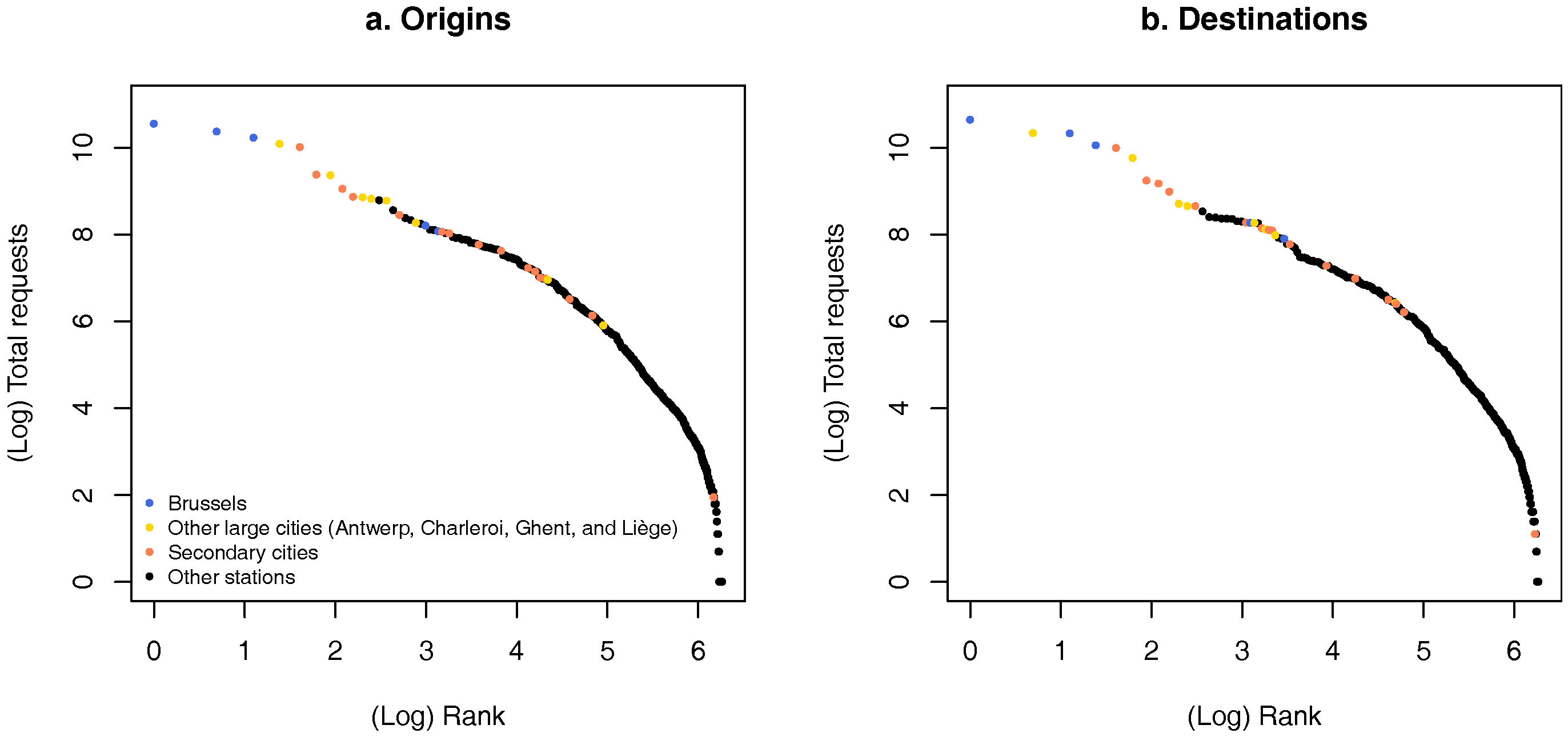
The central node of a community corresponds in most cases to a major city (Table A1), and these cities are also the most frequent nodes in the iRail dataset, both as origins and as destinations (Figure 4). Since the Louvain method ensures that the communities are composed of train stations that have relatively strong interactions with each other, the communities can, therefore, be considered as “influence areas”, similar in their principles to Reilly’s market areas [64]. Note that the stability of the community at the node level (Figure A1) allows assessing the robustness of these catchment areas.

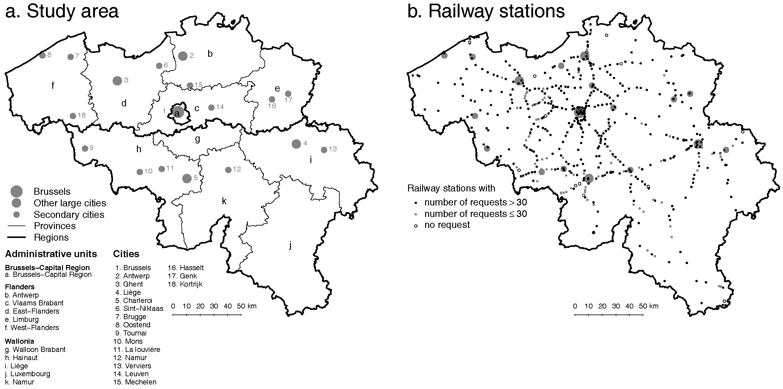
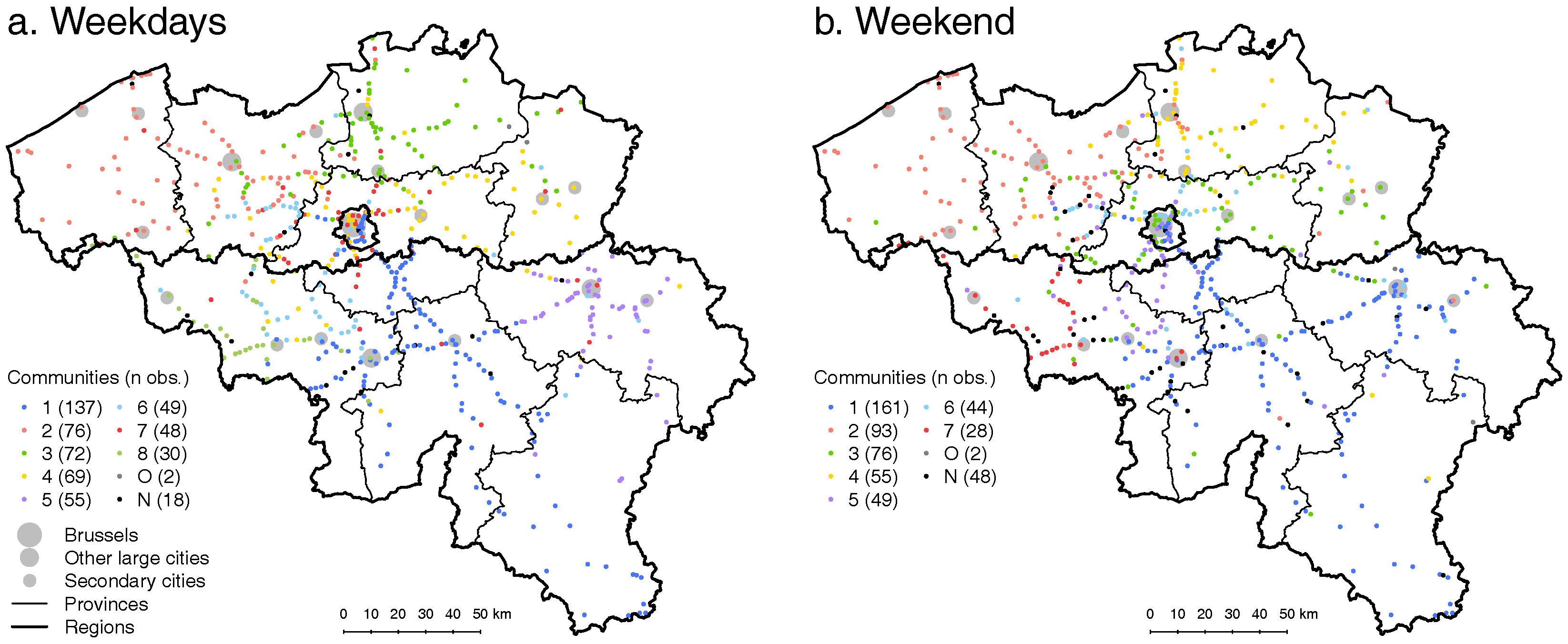
Belgian cities, however, vary in size (see Section 3), and the different data subsets presented in Section 4 also suggest a multi-level structure of the travel demand. This is in particular the case for the no Brussels, weekdays and weekend subsets. Brussels, the largest Belgian city, is the only metropolitan area constituting the central node of more than one community, for all subsets (except, obviously, the no Brussels case). Antwerp and Ghent (in Flanders) emerge as the center of one community for most case studies, while in Wallonia, a community centered on Liège is also found, but for only two of the case studies.

Other results, however, differ from what would be expected of urban-oriented communities. The relationship between the size of the city constituting the central node and the size of the community is tenuous. Among large cities, Charleroi is never the center of a community. Regarding smaller cities, despite (or due to) the denser urban structure in Flanders (Figure 2), no other metropolitan area manages to constitute its own community, while in Wallonia, the relatively small city of Namur is the center of the largest community for most case studies.

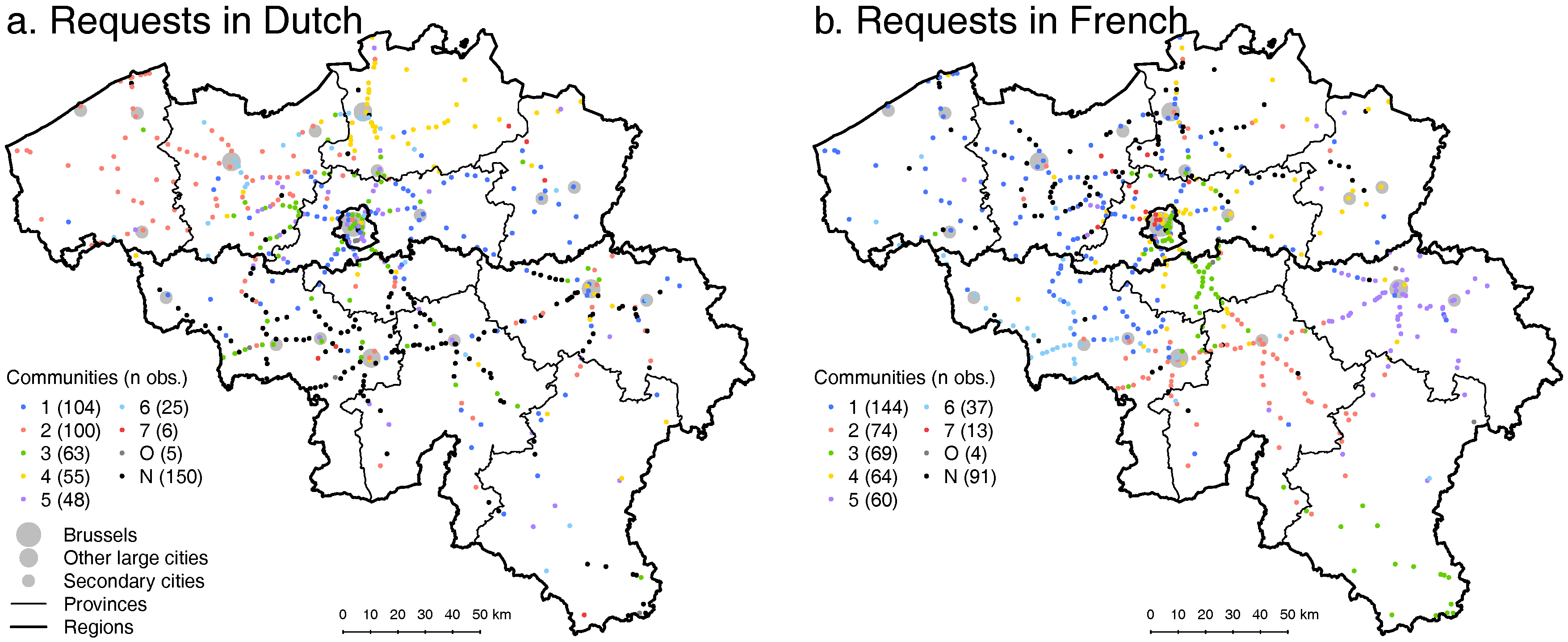
A radial structure centered on Brussels is visible in most data subsets, as well, consistent with a strong influence of the railway network on the communities. This influence seems larger in Wallonia and the eastern part of Flanders, where both the urban structure and railway network are less dense. For instance, the entire Brussels-Namur-Luxembourg line (southeast corner of Belgium) is included in the same community, except for the French subset. In the province of Hainaut (southwest corner), we can also observe communities shaped as triangles, with their basis in that province and their summits in the BCR (for the general, no Brussels and weekend subsets).

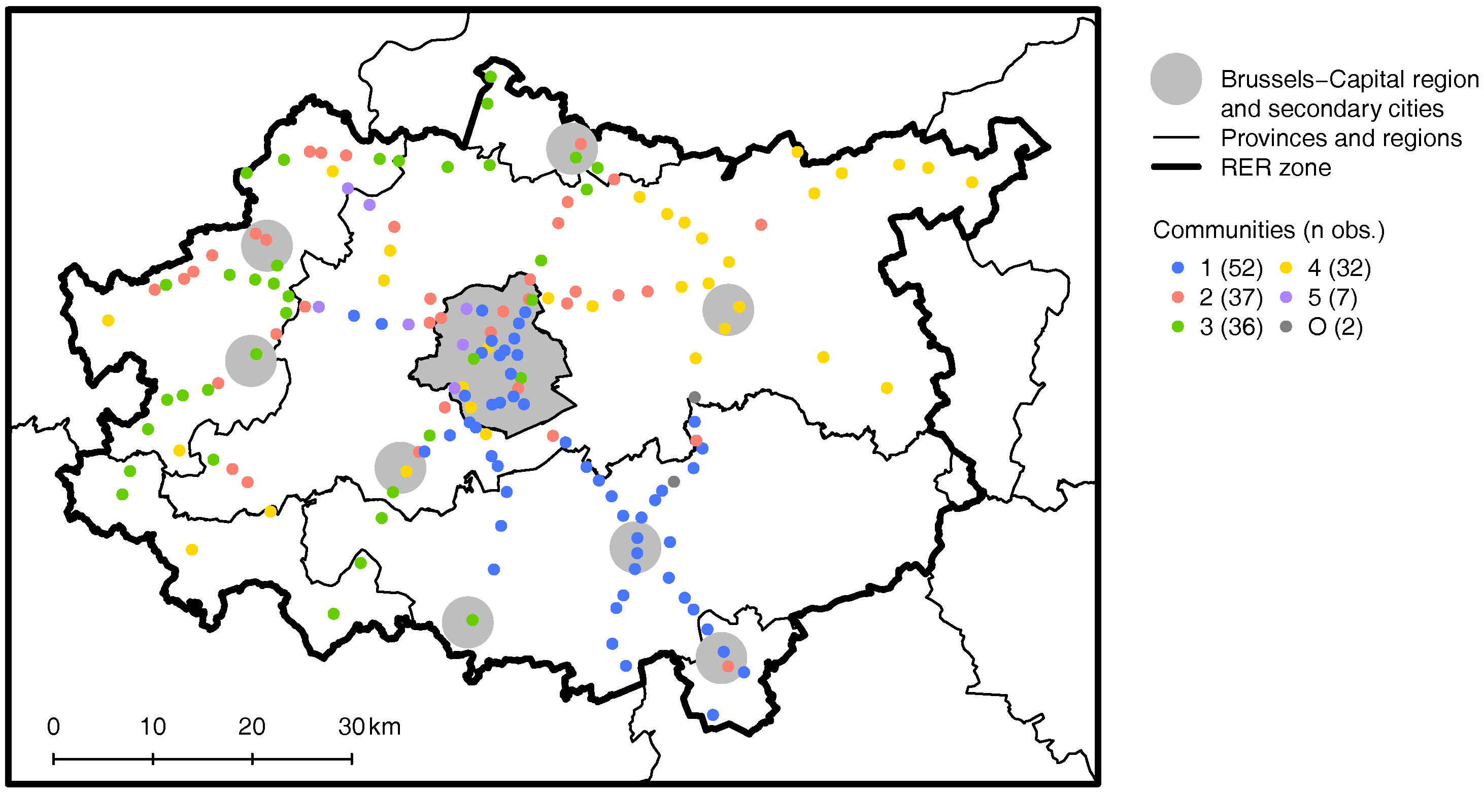
Therefore, both the urban and railway network structures influence the spatial pattern of the communities. More precisely, two factors seem to explain the weight of a city in our results: (1) its size (as expected from the classical gravity model of trade); and (2) its position within the railway network. Brussels is both the largest city of Belgium and the heart of its rail network and is, therefore, an outlier. Antwerp, Ghent and Liège, among other large cities, are main hubs on the network, offering interconnections between several lines. This is less the case for Charleroi (to be precise, we refer here to the stations of Antwerp-Central, Liège-Guillemins, Gent-Sint-Pieters and Charleroi-Sud), the only city that does not emerge as a community center. On the contrary, hubs of the railway network located in smaller cities (as Namur for the French subset) or even a purely functional hub (such as Ottignies for the RER subset) can still constitute communities’ centers. In particular, it is remarkable that for the RER subset all stations close to the Ottignies junction belong to the same community, while this is not the case for relatively larger cities, such as Aalst, Mechelen or Termonde. Both factors (the size of a city and its position on the railway network) are consistent with the economic and transportation geography literature and should be valid for other railway networks than the Belgian one.

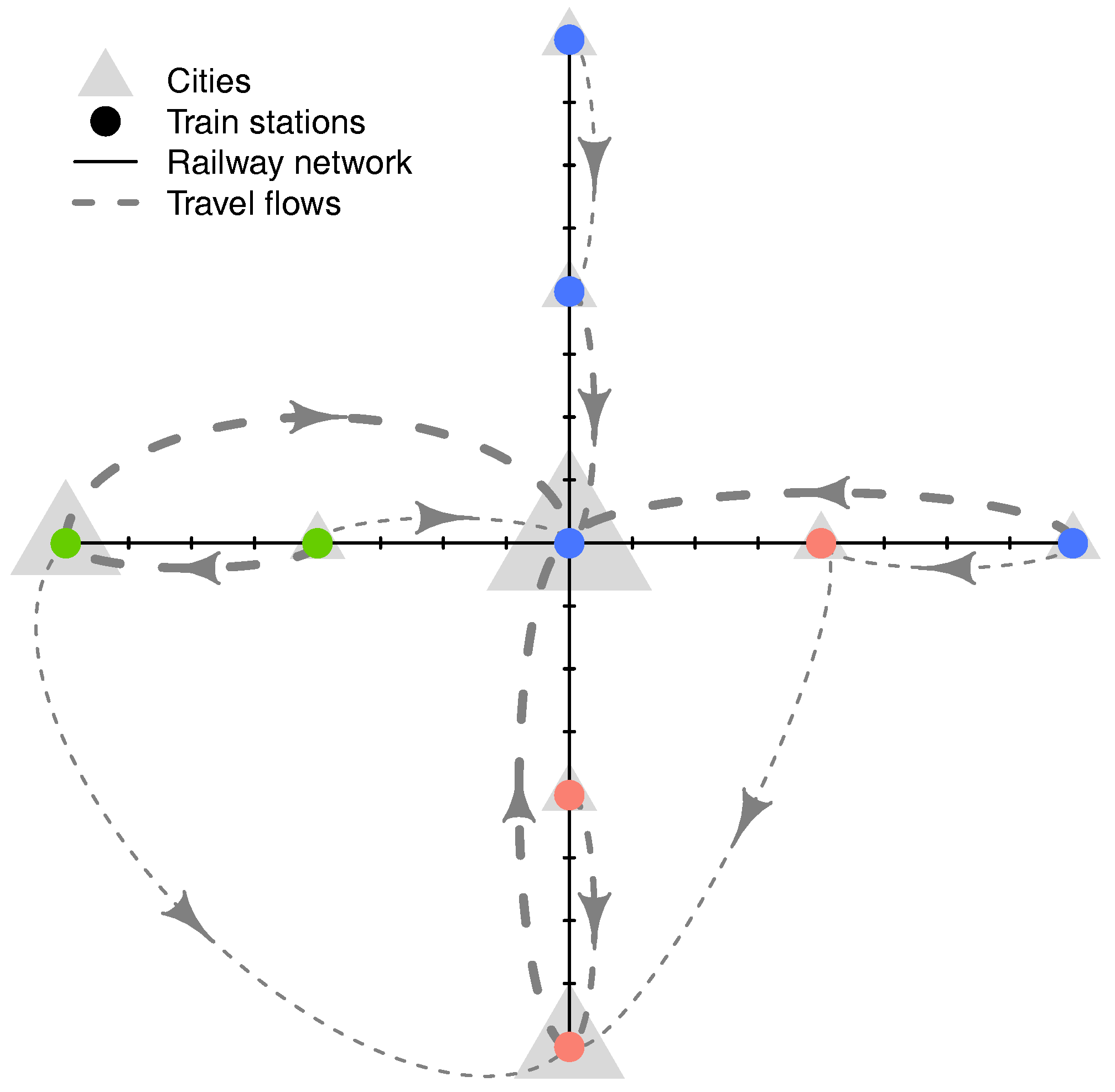
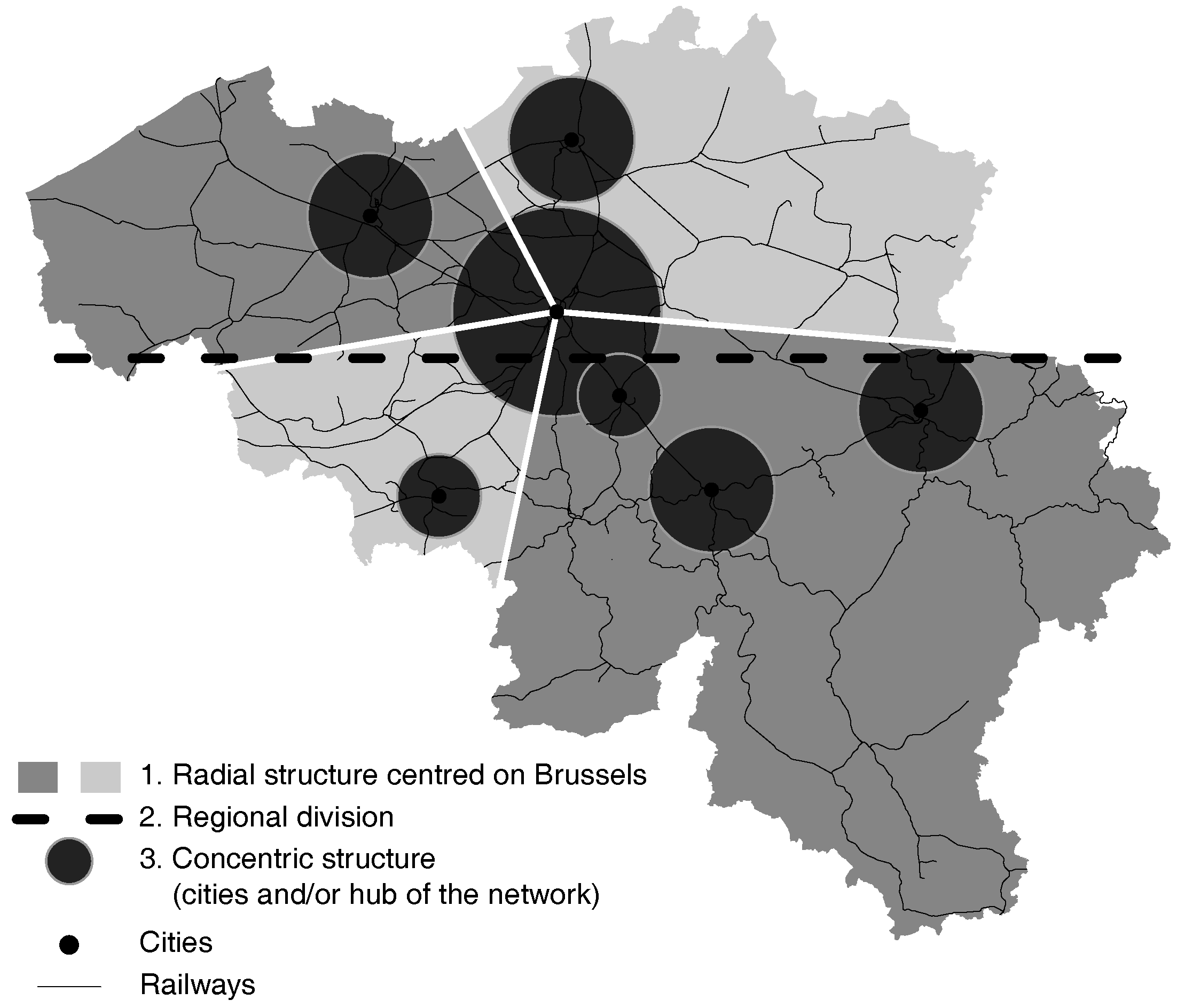
Overall, the spatial structure of the travel demand by train in Belgium, as revealed by the iRail dataset, consists of three nested layers: first, a radial structure centered on Brussels; second, a regional division appears, alongside the linguistic border between Flanders and Wallonia; third, there is a concentric structure around the main hub of the train network, mostly consisting of urban areas. This multi-level organization is schematized in Figure 9. Note that its purpose is to formalize the spatial structure rather than representing the exact extension of the influence area of each city. For instance, the area in-between Brussels and Ghent (on the northwest) is essentially mixed, and the community centered on Ghent extends only to the West of that city. Nevertheless, Ghent is found to be a community center for five of the seven subsets. In our opinion, it deserves therefore its own circle in Figure 9.

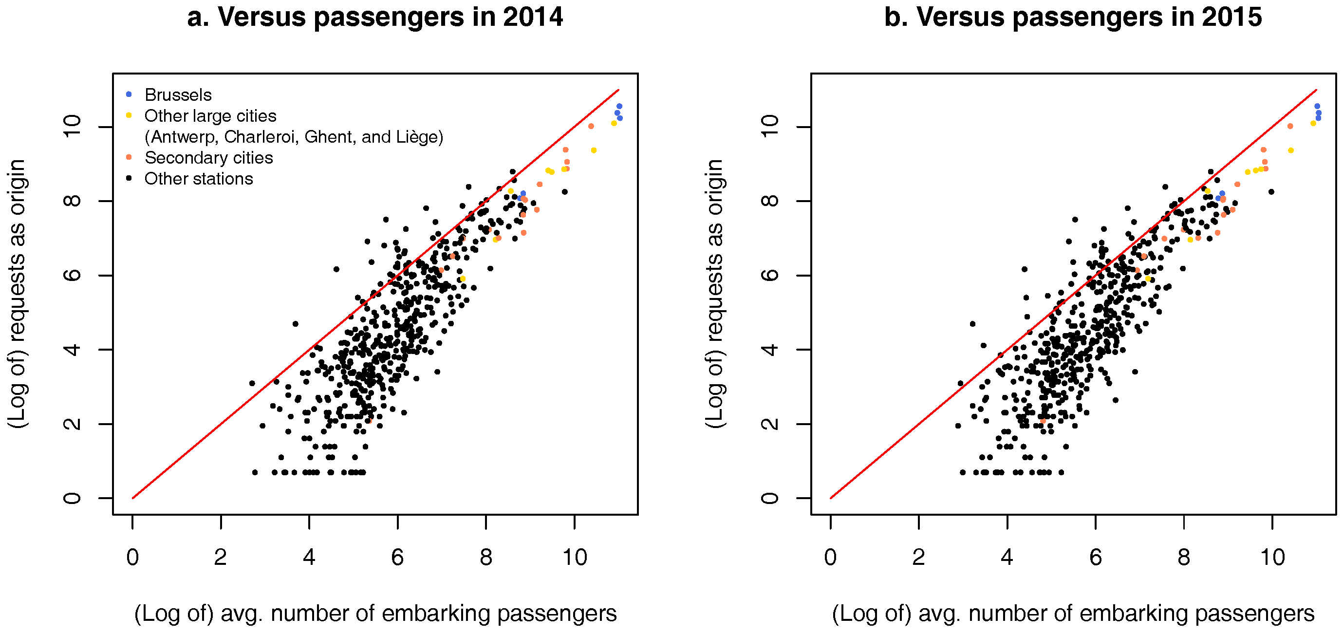
These findings are consistent with our initial hypothesis that both the urban and the railway network structure will influence the travel demand by train in Belgium. They also show that even in a dense country with relatively efficient public transport, such as Belgium, distance is still a key factor of the travel behavior, as assumed by the gravity model of trade and the related theory of market areas. Chiefly, however, their consistency with existing work on the urban and commuting structure of Belgium [26,27,28] constitutes a strong support to our assumption that travel requests provide an accurate depiction of the geography of the actual travel flows.

5.2. Implications for Policy Decisions

The results presented in Section 5.1 are straightforward for anyone familiar with the Belgian context, therefore supporting the robustness of the iRail dataset. Travel requests can thus be used further to explore non-trivial questions regarding transportation planning. In particular, two main debates exist currently in Belgium on the future of the SNCB. The first one concerns the RER service. Due to budgetary constraints, the completion of the network around Brussels (extension from two to four tracks per line) is, as of July 2016, uncertain for the Brussels-Nivelles and Brussels-Ottignies lines [62,65]. Our results show that these two lines belong to a community, including many stations located inside the BCR, both for the general case and for the RER subset (Figure 8). Moreover, the five main stations of Brussels (Brussels-South, Brussels-Central, Brussels-North, Brussels-Schuman and Brussels-Luxembourg) are the destination of 18% of the requests from Ottignies and 80% from Nivelles. This fully supports the importance of completing the infrastructure as originally planned.

An auxiliary discussion about the RER is that local policy makers from the four other large Belgian cities (Antwerp, Charleroi, Ghent and Liège) advocate, from time to time, for the development of a RER service in their own city [61]. The analyses provided here, although not specifically designed to answer this question, suggest that providing such a service would only make sense in metropolitan areas that are the central node of a community, i.e., Antwerp, Ghent and Liège, but not Charleroi. Among smaller cities, Namur is also a potential candidate.

The second debate on the future of the national railway company, mostly fueled by policy makers from Flanders, is its possible separation into two regional (Flanders and Wallonia) companies [66,67]. Our findings do indeed show that most communities do not trespass the linguistic border. This regional division is, however, the second level of the spatial structure described in Section 5.1, the main one being a radial structure centered on Brussels. The spatial pattern of most communities centered on that city is independent from the regional boundaries. Moreover, the five main train stations within the BCR are the destination of travel requests from 423 different stations (or 78% of all stations) and the origins of travel requests towards 431 stations (80%). Whatever the future institutional organization of the Belgian railways, there is thus a clear need to preserve a high level of service to and from Brussels.

Nevertheless, we can question some features of the rail transport offer. In particular, thanks to the “Jonction Nord-Midi” (see Section 3), the main stations in Brussels are connected to each other. Different train services can thus call in Brussels while joining other cities, for instance IC-01 (“IC” stands for “intercity”, i.e., fast interurban connections.) connection links Oostend to Eupen, via Ghent, Brussels and Liège (and vice versa) or the IC-05 connection going from Charleroi to Antwerp, via Brussels. In the iRail dataset, 11% of the requests from Ghent-Sint-Pieters have Brussels-Central as the destination, while for Liège, it is only 0.2%. The corresponding values from Liège-Guillemins are 5% and 0.5%. From the station of Charleroi-Sud, 12% of the requests have Brussels-Central as the destination, and 2% to Antwerpen-Centraal. In the other direction, the shares are 9% for Brussels-Central and 0.7% for Charleroi. Both examples show that the travel demand between two Belgian cities separated by the linguistic border is low, even if a direct connection exists between these towns. One may argue that a train service from a regional city to Brussels and return would be more efficient. However, assessing this question overcomes the goals of this paper.

5.3. Challenges and Paths for Future Research

The first contribution of this paper, as stated by Section 1, was to assess if datasets made of travel requests can represent actual travel flows. Our results confirm their potential, even if the iRail dataset raises two main methodological challenges that should be addressed. First, as detailed in Section 2, a travel request made on the iRail website or application does not mean that the journey was actually made. The number of requests cannot, therefore, be easily translated into forecasts of the absolute number of passengers. Still, using data collected during a two-month period only, we end up with an accurate representation of the relative importance of each link, which is sufficient to study the spatial structure of the travel demand by train in Belgium. The second difficulty is that iRail is only one of the various schedule-finder websites and applications existing for Belgian railways. The analysis proposed in this paper would gain from relying on the travel requests made on the official SNCB application, even if the pattern observed here is consistent with the geography of Belgium.

We were unable to find any published work relying on travel requests to study the travel demand. Nevertheless, datasets similar to iRail exist for all schedule-finder websites or applications, the main issue being their limited availability due to privacy or commercial reasons. Nevertheless, the results presented here open new avenues for further geographical research based on datasets similar to the iRail one.

A first direction for future works is territorial planning. The travel requests allow a high level of spatial and temporal details. In a sustainable development context, they could be used to assess the location of a proposed infrastructure offering the highest willingness to travel by train (or by other public transport means) and the optimal schedules to maximize the modal share of public transport towards this infrastructure.

The second path for research is that ICT data on travels’ intentions, such as the iRail dataset, offer information complementary to datasets on observed travel flows, that could lead to prospective transportation planning. Let us recall that the analyses conducted here rely on the date of the request, reducing the usability of the data to assess temporal variations of the travel demand. In the context of “smart cities” [68], the dataset would benefit from the inclusion in a more robust way of the date and time of the requested journey. A surge of requests towards a given destination (e.g., the Belgian coast) may for instance be used by the SNCB as an indicator that the train’s offer should be increased at the time of the requested journeys (rather than relying solely on weather forecasts). Further work is however requested before being able to forecast trains’ frequentation in the future based on travel requests.

6. Conclusions

This paper shows that travel requests made through an online application provide an accurate view of the travel demand by train in Belgium. Using community-detection methods at the station level, we demonstrate the influence of both the urban and railway network structures on the spatial pattern of the travel demand. The results are consistent with commuting in Belgium. A multi-level structure emerges, consisting of a radial structure centered on Brussels, a regional division between Dutch- and French-speaking areas of Belgium and a concentric structure around cities. The importance of secondary cities depends on the temporal, linguistic or regional subset considered.

The study conducted here shows the relevance of “big data” datasets for geography and regional sciences, since ICT offer numerous ways to collect (real time) data on travel behavior. The analyses proposed here also have direct implications for transportation planning, even if further work is needed to ensure their geographical consistency before being able to fully exploit the potential of journeys’ requests datasets for prospective transport or territorial planning. Nevertheless, the main result is that the spatial structures emerging from our analyses remain consistent with “good old” geographical theories, especially the gravity model of trade and Reilly’s market areas. In our opinion, “big data” should thus not be seen as substitutes or competitors of theoretical models, but rather as an opportunity to look at these theories in an original and innovative way.

References

1. Klapka, P.; Halás, M.; Erlebach, M.; Tonev, P.; Bednar, M. A multistage agglomerative approach for defining functional region of the Czech republic: The use of 2001 commuting data. Morav. Geogr. Rep. 2014, 22, 2–13. [Google Scholar]
2. Farmer, C.; Fotheringham, A.S. Network-based functional regions. Environ. Plan. A 2011, 43, 2723–2741. [Google Scholar] [CrossRef]
3. Konjar, M.; Lisec, A.; Drobne, S. Methods for delineation of functional regions using data on commuters. In Proceedings of the 13th AGILE International conference on Geographic Information Science, Guimaraes, Portugal, 11–14 May 2010.
4. Coombes, M. From City-region concept to boundaries for governance: The English case. Urban Stud. 2013, 52, 1113–1133. [Google Scholar] [CrossRef]
5. Thomas, I.; Cotteels, C.; Jones, J.; Peeters, D. Revisiting the Extension of the Brussels urban agglomeration: New methods, new data... new results? e-Belgeo 2013, 1–2, 1–11. [Google Scholar] [CrossRef]
6. Thomopoulos, N.; Givoni, M.; Rietveld, P. ICT for Transport: Opportunities and Threats; Edward Elgar Publishing: Cheltenham, UK, 2015. [Google Scholar]
7. Kitchin, R. The Data Revolution: Big Data, Open Ddata, Data Infrastructures and Their Consequences; Sage: Thousand Oaks, CA, USA, 2014. [Google Scholar]
8. Vanoutrive, T.; Malderen, L.V.; Jourquin, B.; Thomas, I.; Verhetsel, A.; Witlox, F. Rail commuting to workplaces in Belgium: A multilevel approach. Int. J. Sustain. Transp. 2012, 6, 67–87. [Google Scholar] [CrossRef] [Green Version]
9. Bergstrand, J.H. The gravity equation in international trade: Some microeconomic foundations and empirical evidence. Rev. Econ. Stat. 1985, 67, 474–481. [Google Scholar] [CrossRef]
10. Grasland, C.; Beauguitte, L. Modelling attractiveness of global places: A worldwide survey on 9000 undergraduate students. In Proceedings of the 50th European Congress of the Regional Science Association International on: Sustainable Regional Growth and Development in the Creative Knowledge Economy, Jönköping, Sweden, 19–23 August 2010.
11. Giraud, T.; Commenges, H. SpatialPosition: Spatial Position Models. R Package Version 1.0. 2015. Available online: http://CRAN.R-project.org/package=SpatialPosition (accessed on 9 September 2016).
12. Cervero, R.; Wu, K.L. Polycentrism, commuting, and residential location in the San Francisco Bay area. Environ. Plan. A 1997, 29, 865–886. [Google Scholar] [CrossRef] [PubMed]
13. Wang, F. Modeling commuting patterns in Chicago in a GIS environment: A job accessibility perspective. Prof. Geogr. 2000, 52, 120–133. [Google Scholar] [CrossRef]
14. Wang, F. Explaining intraurban variations of commuting by job proximity and workers’ characteristics. Environ. Plan. B Plan. Des. 2001, 28, 169–182. [Google Scholar] [CrossRef]
15. Sohn, J. Are commuting patterns a good indicator of urban spatial structure? J. Transp. Geogr. 2005, 13, 306–317. [Google Scholar] [CrossRef]
16. Mathä, T.; Wintr, L. Commuting flows across bordering regions: A note. Appl. Econ. Lett. 2009, 16, 735–738. [Google Scholar] [CrossRef]
17. Dujardin, C. Effet de frontière et intégration spatiale: Les migrations alternantes et la frontière linguistique en Belgique. L’espace Géogr. 2001, 2001, 307–320. [Google Scholar]
18. Rodrigue, J.P.; Comtois, C.; Slack, B. The Geography of Transport Systems; Routledge: London, UK, 2013. [Google Scholar]
19. Spiekermann, K.; Wegener, M. The shrinking continent: New time—space maps of europe. Environ. Plan. B Plan. Des. 1994, 21, 653–673. [Google Scholar] [CrossRef]
20. Spiekermann, K.; Wegener, M. Trans-European networks and unequal accessibility in Europe. Eur. J. Reg. Dev. 1996, 4, 35–42. [Google Scholar]
21. Vickerman, R. High-speed rail in Europe: Experience and issues for future development. Ann. Reg. Sci. 1997, 31, 21–38. [Google Scholar] [CrossRef]
22. Givoni, M. Development and impact of the modern High-speed train: A review. Transp. Rev. 2006, 26, 593–611. [Google Scholar] [CrossRef]
23. Levinson, D.M. Accessibility impacts of high-speed rail. J. Transp. Geogr. 2012, 22, 288–291. [Google Scholar] [CrossRef]
24. Blondel, V.; Guillaume, J.L.; Lambiotte, R.; Lefebvre, E. Fast unfolding of communities in large network. J. Stat. Mech. Theory. Exp. 2008, 2008, 10008. [Google Scholar] [CrossRef]
25. Guimera, R.; Mossa, S.; Turtschi, A.; Amaral, L.N. The worldwide air transportation network: Anomalous centrality, community structure, and cities’ global roles. Proc. Natl. Acad. Sci. USA 2005, 102, 7794–7799. [Google Scholar] [CrossRef] [PubMed]
26. Verhetsel, A.; Van Hecke, E.; Halleux, J.M.; Decroly, J.M.; Merenne-Schoumaker, B. Noyaux D’habitats et région Urbaines Dans Une Belgique Urbanisée; Technical Report, Monographie de L’enquète Socio-Économique 2001; SPF Economie: Brussels, Belgium, 2009.
27. Van Hecke, E.; Thomas, I.; Beelen, M.; Halleux, J.M.; Lambotte, J.M.; Rixhon, G.; Verhetsel, A. Le Mouvement Pendulaire en Belgique; Technical Report, Monographie de L’enquète Socio-Économique 2001; SPF Economie: Brussels, Belgium, 2009.
28. Verhetsel, A.; Thomas, I.; Beelen, M. Commuting in Belgian metropolitan areas. J. Transp. Land Use 2010, 2, 109–131. [Google Scholar] [CrossRef]
29. Federal Highway Administration. National Household Travel Survey 2016. Available online: https://www.nationalhouseholdtravelsurvey.com/l (accessed on 9 September 2016).
30. Cornelis, M. Belgian Daily Mobility-BELDAM. 2012. Available online: http://www.belspo.be/belspo/organization/Publ/pub_ostc/agora/ragjj150_fr.pdf (accessed on 9 September 2016).
31. Ahem, A.; Weyman, G.; Redelbach, M.; Schulz, A.; Akkermans, L.; Vannacci, L.; Anoyrkati, E.; van Grinsven, A. Analysis of National Travel Statistics in Europe. 2013. Available online: http://publications.jrc.ec.europa.eu/repository/bitstream/JRC83304/tch-d2.1_final.pdf (accessed on 9 September 2016).
32. Hubert, J.P.; Armoogum, J.; Axhausen, K.W.; Madre, J.L. Immobility and mobility seen through trip-based versus time-use surveys. Transp. Rev. 2008, 28, 641–658. [Google Scholar] [CrossRef]
33. Gerike, R.; Gehlert, T.; Leisch, F. Time use in travel surveys and time use surveys—Two sides of the same coin? Transp. Res. Part A Policy Prac. 2015, 76, 4–24. [Google Scholar] [CrossRef]
34. Roth, C.; Kang, S.M.; Batty, M.; Barthelemy, M. Structure of urban movements: Polycentric activity and entangled hierarchical flows. PLoS ONE 2011, 6, e15923. [Google Scholar] [CrossRef] [PubMed]
35. Long, Y.; Thill, J. Combining smart card data and household travel survey to analyze jobs-housing relationships in Beijing. Comput. Environ. Urban Syst. 2015, 53, 19–35. [Google Scholar] [CrossRef]
36. Sun, S.; Duan, Z.; Yang, D.; Li, W. Polycentricity of the urban structure: Spatial movements analysis in Shanghai with smart card data. In Proceedings of the 21st World Congress on Intelligent Transport Systems, ITSWC 2014: Reinventing Transportation in Our Connected World, Detroit, MI, USA, 7–11 September 2014.
37. SNCB. Available online: http://www.belgianrail.be/en (accessed on 9 November 2016).
38. DGSIE. Population—Chiffres Population 2010–2016. Available online: http://statbel.fgov.be/fr/modules/publications/statistiques/population/population_-_chiffres_population_2010_-_2012.jsp (accessed on 9 September 2016).
39. Thisse, J.F.; Thomas, I. Bruxelles au sein de l’économie belge: Un bilan. Reflets Perspect. Econ. 2010, 80, 1–18. [Google Scholar]
40. Van der Herten, B. Le Temps du Train, 175 ans de Chemins de fer en Belgique, 75e Anniversaire de la SNCB; Presses Universitaires de Louvain: Louvain la Neuve, Belgium, 2001. [Google Scholar]
41. Denis, J. (Ed.) Geographie de la Belgique; Bulletin du Credit Communal: Brussels, Belgium, 1992; p. 616.
42. National Geography Committee. A Concise Geography of Belgium; Academia Press: Ghent, Belgium, 2012; p. 46. [Google Scholar]
43. Infrabel. Railway Lines. Available online: http://www.infrabel.be/en/about/our-rail-network/railway-lines (accessed on 9 September 2016).
44. SNCB. SNCB 2015 Activities Report. 2015. Available online: http://www.belgianrail.be/en/corporate/~/media/1212C2ABEFCA4BC0A236781FECE168E5.ashx (accessed on 9 September 2016).
45. iRail. Available online: https://irail.be/ (accessed on 9 November 2016).
46. iRail API. Available online: https://hello.irail.be/api/1-0/ (accessed on 9 November 2016).
47. Colpaert, P.; Chua, A.; Verborgh, R.; Mannens, E.; Van de Walle, R.; Vande Moere, A. What public transit API logs tell us about travel flows. In Proceedings of the 25th International Conference Companion on World Wide Web. International World Wide Web Conferences Steering Committee, Montreal, QC, Canada, 11–15 April 2016; pp. 873–878.
48. SNCB. Nombre de Voyageurs Montes Par Gare en 2014. Available online: https://www.belgianrail.be/fr/~/media/73AECBB3473141C1AA565C122AB6259C.ashx (accessed on 9 September 2016).
49. SNCB. Nombre de Voyageurs Montes Par Gare en 2015. Available online: http://www.belgianrail.be/fr/~/media/8F764D77F60F48B188A8742652C6E48F.ashx (accessed on 9 September 2016).
50. Delvenne, J.C.; Schaub, M.T.; Yaliraki, S.N.; Barahona, M. The stability of a graph partition: A dynamics-based framework for community detection. In Dynamics On and Of Complex Networks; Springer: Berlin, Germany, 2013; Volume 2, pp. 221–242. [Google Scholar]
51. Lancichinetti, A.; Radicchi, F.; Ramasco, J.J.; Fortunato, S. Finding statistically significant communities in networks. PLoS ONE 2011, 6, e18961. [Google Scholar] [CrossRef] [PubMed]
52. Traag, V.; Van Dooren, P.; Nesterov, Y. Narrow scope for resolution-limit-free community detection. Phys. Rev. E 2011, 84, 016114. [Google Scholar] [CrossRef] [PubMed]
53. Traag, V.A.; Krings, G.; Van Dooren, P. Significant scales in community structure. Sci. Rep. 2013, 1–10. [Google Scholar] [CrossRef] [PubMed]
54. Lee, C.; Cunningham, P. Community detection: Effective evaluation on large social networks. J. Complex Netw. 2014, 2, 19–37. [Google Scholar] [CrossRef]
55. Good, B.H.; de Montjoye, Y.A.; Clauset, A. Performance of modularity maximization in practical contexts. Phys. Rev. E 2010, 81, 046106. [Google Scholar] [CrossRef] [PubMed]
56. Ana, L.; Jain, A.K. Robust data clustering. In Proceedings of the 2003 IEEE Computer Society Conference on Computer Vision and Pattern Recognition, Madison, WI, USA, 18–20 June 2003; Volume 2.
57. Freeman, L.C. A set of measures of centrality based on betweenness. Sociometry 1977, 40, 35–41. [Google Scholar] [CrossRef]
58. Blondel, V.; Krings, G.; Thomas, I. Regions and borders of mobile telephony in Belgium and in the Brussels metropolitan zone. Brussels Stud. 2010, 42, 1–12. [Google Scholar]
59. De Witte, A.; Macharis, C.; Mairesse, O. How persuasive is free public transport?: A survey among commuters in the Brussels Capital Region. Transp. Policy 2008, 15, 216–224. [Google Scholar] [CrossRef]
60. Vandenbulcke, G.; Dujardin, C.; Thomas, I.; de Geus, B.; Degraeuwe, B.; Meeusen, R.; Panis, L.I. Cycle commuting in Belgium: Spatial determinants and share-cycling strategies. Transp. Res. Part A Policy Pract. 2011, 45, 118–137. [Google Scholar] [CrossRef]
61. SNCB. S-Train. Available online: http://www.belgianrail.be/en/ /media/91715610D054471E8B2D70D3CD3B6562.pdf (accessed on 9 September 2016).
62. J.C. RER a Bruxelles: Quel etait le projet? Qu’en est-il maintenant? Available online: https://www.rtbf.be/info/regions/bruxelles/detail_rer-a-bruxelles-quel-etait-le-projet-qu-en-est-il-maintenant?id=9202743 (accessed on 9 September 2016).
63. Ordonnance Portant Assentiment à la Convention du 4 Avril 2003 Entre l’Etat fédéral, la Région Flamande, la Région Wallone et la Région de Bruxelles-Capitale, Visant à mettre en Oeuvre le Programme du Réseau Express R’egional de, Vers, Dans et Autour de Bruxelles; Moniteur Belge: Brussels, Belgium, 2004.
64. Huff, D.L. A probabilistic analysis of shopping center trade areas. Land Econ. 1963, 39, 81–90. [Google Scholar] [CrossRef]
65. Attout, X. RER: Scenario catastrophe en vue? Le Soir 2016. Available online: http://www.lesoir.be/1264492/article/actualite/regions/brabant-wallon/2016-07-12/rer-scenario-catastrophe-en-vue (accessed on 9 September 2016).
66. Jan Peumans (N-VA): Il serait bon de regionaliser la SNCB. Le Soir 2015. Available online: http://www.lesoir.be/933608/article/actualite/belgique/politique/2015-07-11/jan-peumans-n-vail-serait-bon-regionaliser-sncb (accessed on 9 September 2016).
67. RTBF. Une Regionalisation de la SNCB Est-Elle Possible? Available online: https://www.rtbf.be/info/belgique/detail_une-regionalisation-de-la-sncb-est-elle-realisable?id=9178419 (accessed on 9 September 2016).
68. Kitchin, R. The real-time city? Big data and smart urbanism. GeoJournal 2014, 79, 1–14. [Google Scholar] [CrossRef]
Figure 1. Illustration of railway network versus travel-demand network (city and travel flow symbols proportional to their size/volume; the color of each train station represents its community).
Ijgi 05 00216 g001
Figure 2. (a) Administrative and urban structure of Belgium; and (b) location of the train station.
Ijgi 05 00216 g002
Figure 3. iRail requests versus observed travel demand. (a) Versus passengers in 2014; (b) Versus passengers in 2015.
Ijgi 05 00216 g003
Figure 4. Rank - size distribution of the iRail requests. (a) Origins; (b) Destinations.
Ijgi 05 00216 g004
Figure 5. Communities in the iRail dataset for the (a) general and (b) no Brussels subsets (in the legend: O = other communities, with less than five nodes; N = not present in the dataset).
Ijgi 05 00216 g005
Figure 6. Communities detected in the iRail dataset during (a) weekdays and (b) weekends (in the legend: O = other communities, with less than five nodes; N = not present in the dataset).
Ijgi 05 00216 g006
Figure 7. Communities in the iRail dataset for the requests made in (a) Dutch and in (b) French (in the legend: O = other communities, with less than five nodes; N = not present in the dataset).
Ijgi 05 00216 g007
Figure 8. Communities detected within the RER zone (note: O = other communities, with less than five train stations).
Ijgi 05 00216 g008
Figure 9. Chorematic representation of the travel demand by train in Belgium.
Ijgi 05 00216 g009