Article

Combined Forecasting Method of Landslide Deformation Based on MEEMD, Approximate Entropy, and WLS-SVM

1
College of Geomatics and Geoinformation, Guilin University of Technology, Guilin 541004, China
2
Research Center of Precise Engineering Surveying, Guangxi Key Laboratory of Spatial Information and Geomatics, Guilin 541004, China
*
Authors to whom correspondence should be addressed.
ISPRS Int. J. Geo-Inf. 2017, 6(1), 5; https://0-doi-org.brum.beds.ac.uk/10.3390/ijgi6010005
Submission received: 12 October 2016 / Accepted: 19 December 2016 / Published: 1 January 2017
(This article belongs to the Special Issue Recent Advances in Geodesy & Its Applications)

Abstract

:
Given the chaotic characteristics of the time series of landslides, a new method based on modified ensemble empirical mode decomposition (MEEMD), approximate entropy and the weighted least square support vector machine (WLS-SVM) was proposed. The method mainly started from the chaotic sequence of time-frequency analysis and improved the model performance as follows: first a deformation time series was decomposed into a series of subsequences with significantly different complexity using MEEMD. Then the approximate entropy method was used to generate a new subsequence for the combination of subsequences with similar complexity, which could effectively concentrate the component feature information and reduce the computational scale. Finally the WLS-SVM prediction model was established for each new subsequence. At the same time, phase space reconstruction theory and the grid search method were used to select the input dimension and the optimal parameters of the model, and then the superposition of each predicted value was the final forecasting result. Taking the landslide deformation data of Danba as an example, the experiments were carried out and compared with wavelet neural network, support vector machine, least square support vector machine and various combination schemes. The experimental results show that the algorithm has high prediction accuracy. It can ensure a better prediction effect even in landslide deformation periods of rapid fluctuation, and it can also better control the residual value and effectively reduce the error interval.

1. Introduction

Slope displacement and instability are often encountered in natural and artificial slopes as deformation phenomena. They have important significance in slope stability evaluation, slope safety early warning, and slippery slope hazard control for timely grasping of the slope deformation evolution rules and accurate prediction of future evolution rules and trends of slope deformation [1,2,3,4,5,6,7,8]. Currently the main methods of landslide deformation prediction include Grey models, neural networks, support vector machine (SVM), least squares support vector machine (LS-SVM), and a variety of combinations of forecasting methods [5,6,7,8,9]. When the original data sequence fluctuation is large and the information is too dispersed, the prediction accuracy of Grey theory is relatively low. Neural network models have defects that are difficult to overcome, such as easily becoming trapped into local minima, difficulties in determining network structure, and a prerequisite to the successful application that the dynamic mechanism of the system has relative consistency. With the emergence of a new type of general learning algorithm, SVM, which is based on small sample size and statistical learning theory [9,10], many scholars have applied it in deformation prediction and achieved good results. Zhao et al. [11] applied SVM in deformation prediction and they solved the problem of complex deformation prediction under multi-factor impact so that its accuracy was better than that of the traditional forecasting methods. However SVM has limitations of slow computing speed and weak robustness. LS-SVM as an extension of SVM, can reduce the computational complexity, can speed up the solving speed, and has a strong anti-interference ability, but it loses the standard SVM robustness problem [12,13]. Due to the combined effects of groundwater, human activities and other factors, it is difficult to establish a relatively accurate model of the complex nonlinear relationship between the deformation and the influence factors. The displacement of landslides often has the characteristic of being controlled by the time scale, with a trend of growing at large time scales and having considerable randomness and volatility at small time scales. The fluctuations also have a certain periodicity and regularity at a certain time scale. A landslide displacement time series signal generally consists of the following four parts; the deterministic tendency item, the periodic item, the pulsation item and the random item with uncertainty [14,15,16,17]. The landslide system belongs to a nonlinear energy dissipation system, which shows a very obvious chaotic state in the long-term evolution of the system [14,15,16,17]. From the perspective of time-frequency analysis, Wang et al. [18,19] combined the wavelet decomposition and SVM and applied it in deformation prediction. This prediction model could further improve the prediction accuracy after decomposing deformation series into narrowband signals with different characteristic scales. However the key to wavelet analysis is the selection of the wavelet function and the decomposition scale. It is difficult to avoid the influence of human factors, and it is not easy to achieve the global optimal decomposition of the signal. Therefore, through the chaotic analysis of landslide deformation sequences, digging out the implicit time-frequency information, providing more effective data for modeling prediction, and establishing a reasonable combination model to improve the prediction performance have certain research significance.
Based on the characteristics of landslides and the above research, this paper started from the two aspects of how to effectively separate the time-frequency information of the chaotic sequence and improve the model performance, and we proposed a landslide chaotic time series prediction algorithm based on modified ensemble empirical mode decomposition (MEEMD), approximate entropy and weighted least squares support vector machine (WLS-SVM). First MEEMD [20,21,22] was used to decompose the non-stationary landslide time series into a series of different characteristic scales of intrinsic mode function (IMF). Then the approximate entropy [23,24] was adopted for the complexity analysis of each component, producing a new subsequence through combination stacking according to the different entropy values. Finally WLS-SVM was used to model [12,13] and analyze the new subsequence. At the same time, phase space reconstruction theory [25] and grid search [26] were used to determine the optimal input dimension of the model and the optimal parameters. Taking the Danba landslide deformation data as an experimental example, we compared the wavelet neural network, SVM, LS-SVM and seven other combination schemes, through different prediction steps, to further explore and verify the feasibility and effectiveness of the new algorithm in the landslide’s chaotic sequence.

2. Landslide Prediction Model Based on MEEMD, Approximation Entropy, and WLS-SVM

2.1. Modified Ensemble Empirical Mode Decomposition

By adding white noise to the signal, the ensemble empirical mode decomposition (EEMD) [27] can solve the problem of the boundary effect of traditional empirical mode decomposition to a certain extent, and the real signal can be preserved to the maximal extent. However EEMD also has some of the following problems [28,29]: if the amplitude of white noise added to EEMD is too low it cannot restrain the mixed mode stack well; if it is too large it would increase the average total amount of calculation, easily cause the decomposition of the high-frequency components, and make the white noise residual too large. Moreover the result of EEMD decomposition is not necessarily the standard IMF, but the problem of mode splitting may also occur, that is, the same physical process is divided into multiple IMF components. Therefore, given the chaotic sequence of landslide deformation, this paper uses MEEMD to decompose, and the detailed decomposition process is shown in the literature [20,21,22].

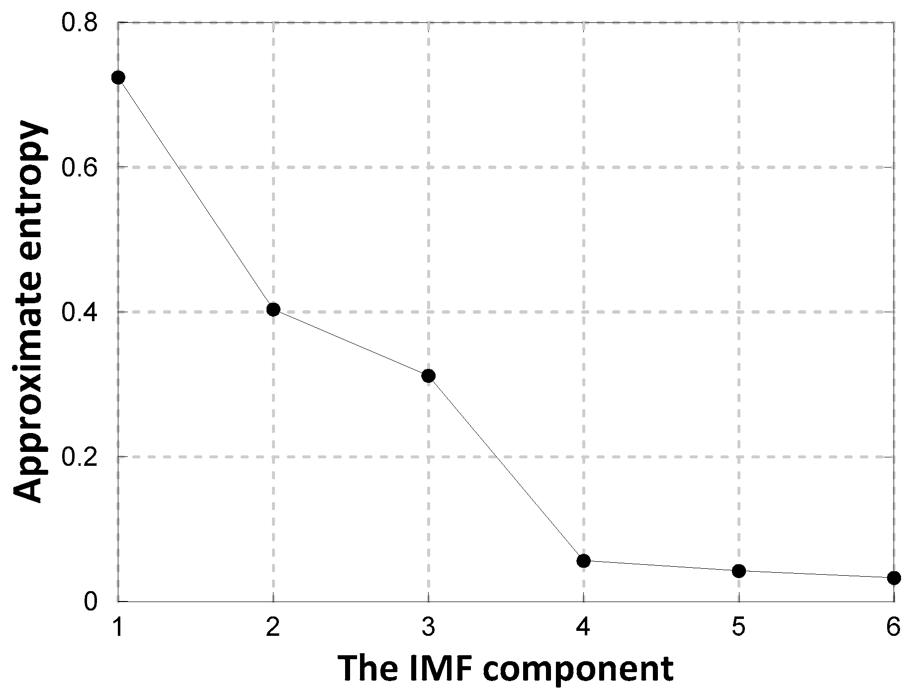
2.2. Approximate Entropy Principle

Pincun et al. [23] proposed the approximate entropy method for measuring the degree of complexity in 1991. This method can yield stable values with less data and is suitable for engineering applications. The value of approximate entropy can reflect the complexity of the sequence. The greater the value is the more complex the sequence is. The detailed calculation steps are as follows [23]:
(1) Setting a landside sequence as { x ( i ) ,   i = 1 , 2 , , n } , constructing an m-dimensional vector according to the sequences order:
X ( i ) = [ x ( i ) , x ( i + 1 ) , x ( i + 2 ) , , x ( i + m 1 ) ] ,   ( i = 1 , 2 , , n m + 1 )
(2) Assume that the maximum difference between X ( i ) and X ( j ) ,   ( j = 1 , 2 , , n m + 1 ,   j i ) is D m [ X ( i ) , X ( j ) ] :
D m [ X ( i ) , X ( j ) ] = max 0 ~ m 1 | x ( i + k ) x ( j + k ) |
Here calculating the distance between vector X ( i ) and other vectors X ( j ) according to i to obtain the maximum distance.
(3) Setting the similar tolerance as r ( r > 0 ) , counting the numbers of D m [ X ( i ) , X ( j ) ] < r , calculating the ratio C i m ( r ) of the numbers of D m [ X ( i ) , X ( j ) ] < r to the total numbers of distance ( n m + 1 ) :
C i m ( r ) = 1 n m + 1 sum { D m [ X ( i ) , X ( j ) ] < r }
Here, ( j = 1 , 2 , , n m + 1 ,   j i ) , sum is the number of D m [ X ( i ) , X ( j ) ] < r .
(4) Calculating the logarithm of C i m ( r ) , and then computing the average ϕ m ( r ) of all i :
ϕ m ( r ) = 1 n m + 1 i = 1 n m + 1 ln C i m ( r )
(5) Adding the dimension to m + 1 , repeating steps (1) to (4), C i m + 1 ( r ) and ϕ m + 1 ( r ) can be obtained.
(6) Setting approximate entropy as A p E n ( m , r ) :
A p E n ( m , r ) = lim n [ ϕ m ( r ) ϕ m + 1 ( r ) ]
Generally n is a finite value, and then the approximate entropy value is obtained:
A p E n ( m , r , n ) = ϕ n ( r ) ϕ m + 1 ( r )
Obviously the value of A p E n relates to m , r and n . Normally the value of A p E n mainly depends on m and r , and less depends on n . Generally m is 2 and r is a value between 0.1   and   0.25 S D , where S D is the standard deviation of sequence. Therefore m is 2 and r is 0.2 S D in this paper.

2.3. Phase Space Reconstruction Theory

Kennel et al. proposed phase space reconstruction theory [25] and introduced chaos theory into the nonlinear time series analysis. Using this method, the nonlinear dynamic characteristics of the deformation sequence of the side slope were excavated. Optimizing the learning samples of the prediction model based on this method has been considered an effective and novel method, which has a certain significance. At the same time, Takens [30] proved that the proper selection of delay time and large enough embedding dimension can make the reconstructed phase space reflect the rule of the system status with time evolution correctly, and it has the same properties as the actual dynamical systems.
For the landslide deformation sequence in this paper, { y ( t ) ,   t = 1 , 2 , , n } , n is the sequence length. According to Takens’ theory, the function f ( · ) exists and the reconstructed phase space is [25]:
Y t + 1 = f ( Y t , Y t τ , , Y t ( m 1 ) τ )
Here τ is the delay time, and m is the number of embedded dimensions.
The correct selection of delay time and embedded dimension directly relates to the accuracy of the reconstruction of the sequence. The common methods are the GP algorithm, the complex self-correlation method, the C-C method and so on. In this paper, the C-C method was used to reconstruct the phase space of each new subsequence. The basic principle of the C-C method is to estimate the time delay τ and the time window τ w ( m 1 ) τ using the correlation integral function of the embedding time series.

2.4. Weighted Least Squares Support Vector Machine

2.4.1. Least Squares Support Vector Machine

Suppose that the given sample training set is { ( x i , y i ) | i = 1 , 2 , , N } . Here x i R n is an n-dimensional input data; R n is an n-dimensional vector space which is composed of real numbers; y i R is an output data and R is a real number. The optimal linear decision function in this space is constructed as follows:
f ( x ) = w T ϕ ( x ) + b
Here ϕ ( x ) : R n R n h is a nonlinear mapping function which maps the input space data to high dimensional feature space, w R n h is the weight vector of original weight space, R n h is a high dimensional space vector composed of real numbers, b R is offset item, and w T is the transpose of vector w .
According to the principle of structural risk minimization (SRM), the objective function Q and constraint condition y i are as follows:
{ min w , b , e Q ( w , e ) = 1 2 w T w + γ 2 i = 1 N e i 2 y i = w T ϕ ( x i ) + b + e i   ( i = 1 , 2 , , N )
Here γ > 0 is the regularization parameter (or penalty coefficient), e i is the error variance, and e is a vector consisted of the error variances.
Introducing the Lagrange multiplier function, α i R , the Lagrange function is obtained as follows:
L ( w , b , e , a ) = Q ( w , e ) i = 1 N a i { w T ϕ ( x i ) + b + e i y i }
Here a = [ a 1 , a 2 , , a N ] T . According to the KKT (Karush–Kuhn–Tucker) condition, the optimal solution is obtained by calculating the partial derivatives of the Lagrange function:
{ L ω = 0     W = i = 1 N a i ϕ ( x i ) L b = 0     i = 1 N a i = 0 L e i = 0     γ e i = a i L a i = 0     w T ϕ ( x i ) + b + e i y i = 0
Through eliminating ω and e in formula (11), the optimization problem is transformed into a linear equation as follows:
[ 0 A T A K ( x k 1 , x k 2 ) + γ 1 I ] [ b a ] = [ 0 y ]
Here y = [ y 1 , y 2 , , y N ] T ; A = [ 1 , , 1 ] T ; I is an N-order identity matrix; and K ( x k 1 , x k 2 ) is a kernel function satisfying the Mercer condition, K ( x k 1 , x k 2 ) N × N . At present, there are 3 kinds of commonly used kernel functions: (1) linear function K ( x k 1 , x k 2 ) = x k 1 T x k 2 ; (2) polynomial function K ( x k 1 , x k 2 ) = ( x k 1 T x k 2 + 1 ) d ,   d = 1 , 2 , ; and (3) radial basis function (RBF) K ( x k 1 , x k 2 ) = exp ( x k 1 x k 2 / 2 σ 2 ) .
Since B = K ( x k 1 , x k 2 ) + γ 1 I is a symmetric positive definite matrix, a and b in formula (12) can be calculated by using least square principle; thus the nonlinear prediction model of LS-SVM is obtained:
y ( x ) = i = 1 N a i K ( x , x i ) + b

2.4.2. Weighted Least Squares Support Vector Machine

LS-SVM converts the quadratic programming problem of SVM to the problem of solving linear equations, which can reduce the computational complexity and improve the solving speed. However LS-SVM has lost its original robustness, which makes the weights of the training samples given by the objective function become the same. That is to say, the role of the sample in training is the same. However, in practice, the characteristics of the data of different samples are different or the influence of various external factors is not the same; therefore the weight in training is not the same. Therefore to regain robustness and establish a more accurate prediction model, this paper uses the improved LS-SVM; that is, the WLS-SVM [12,13]. This model gives different weight factor v i to each error e i = a i / γ on the basis of LS-SVM, so then the optimization problem of the formula (9) is converted to:
{ min w * , b * , e * Q ( w * , e * ) = 1 2 w * T w * + γ 2 i = 1 N v i e i * 2 y i = w * T ϕ ( x i ) + b * + e i *   ( i = 1 , 2 , , N )
The Lagrange function is transformed into:
L ( w * , b * , e * , a * ) = J ( w * , e * ) i = 1 N a i * ( w * T ϕ ( x i ) + b * + e i * y i )
In the same way, the linear equations are obtained as follows:
[ 0 A T A K ( x k 1 , x k 2 ) + V γ ] [ b * a * ] = [ 0 y ]
Here V γ is the diagonal matrix, V γ = d i a g { 1 γ v 1 , , 1 γ v n } . Then;
v i = { 1 ,   | e i / S ^ | c 1 c 2 | e i / S ^ | c 2 c 1 ,   c 1 | e i / S ^ | c 2 10 10 ,   e l s e
Here S ^ is the robust estimation of the standard deviation of the error, which can measure the deviation degree of e i from the following Gaussian distribution; S ^ = I Q R 2 × 0.6745 . I Q R is the interquartile range of the error e i ; that is, after arranging them according to the size of value, the difference between value [ 0.75 n ] and value [ 0.25 n ] . According to the literature [11], c 1 is 2.5 and c 2 is 3.

2.4.3. Parameters Optimization of WLS-SVM

The performance of WLS-SVM is largely determined by the optimal selection of the kernel function k (   ) , the kernel parameter σ , and the regularization parameter γ . Because the RBF can better reflect the complexity of the model and its prediction performance is better. Therefore, this paper selected the RBF as the kernel function of WLS-SVM. Considering the parameter selection problem, the grid search method was used to optimize the parameters, and its basic principle was to divide the mesh grid in a certain range of σ and γ , traverse all of the mesh grid points, and define values. According to the values of σ and γ , the training root mean square error (RMSE) obtained by using the cross-validation method was taken as the objective function of grid point calculation [26]. Finally the ( σ , γ ) values were selected as the optimal parameter by minimizing the RMSE of the training set. The steps of parameter optimization are as follows [26]:
(1)
Setting the value range, the step size, and grid spacing of parameters ( σ , γ ) , the optimization process in this paper is divided into two steps of coarse selection and accurate selection. The parameters are set as follows; the optimization interval of σ and γ is [ 0 , 10 10 ] , the number of grid points is 10 10 × 10 10 , the search step size of coarse selection is 1, and the search step size of accurate selection is 0.1.
(2)
Since the optimization process is a traversal process, the selection of parameter initial value has no effect on the result. The initial values of this search process are σ = 0 and γ = 1 . Selecting the position of the first cross-validation grid point, obtaining the training RMSE using the cross-validation method as the objective function of the grid point calculation, and calculating all of the grid point values.
(3)
Selecting the ( σ , γ ) with the smallest RMSE as the optimal parameters. If the selected parameters cannot satisfy the accuracy requirement, then take the selecting parameters as the center grid point, build a new 2-dimensional grid plane in a smaller range to recalculate the objective function, and select the parameter ( σ , γ ) with the smallest RMSE again as the optimal parameter. If the accuracy requirement is satisfied, stop or repeat the above steps, acquire the accurate parameters ( σ , γ ) , and take them as the optimal values.

2.4.4. Computational Procedure of WLS-SVM

(1)
According to the given sample of landside deformation data { ( x i , y i ) | i = 1 , 2 , , N } , determining the optimal parameter ( σ , γ ) , obtaining a i from formula (12), and then calculating e i = a i / γ ;
(2)
Calculating the robust estimation S ^ according to the distribution of error e i ;
(3)
Determining the corresponding weight values v i according to e i and S ^ through formulation (17);
(4)
Finally a * and b * can be got by formulation (16). Accordingly the final nonlinear prediction model can be obtained as follows:
y ( x ) = i = k 1 N a i * K ( x , x i ) + b *
It can be seen that the LS-SVM calculated from formula (12) is the optimal solution under the assumption that error e i obeys Gaussian distribution, while WLS-SVM corrects the deviation caused by non-Gaussian distribution of error e i through defining the weight in formula (17), which makes WLS-SVM regression robust and improves the prediction accuracy.

3. Analysis of Examples

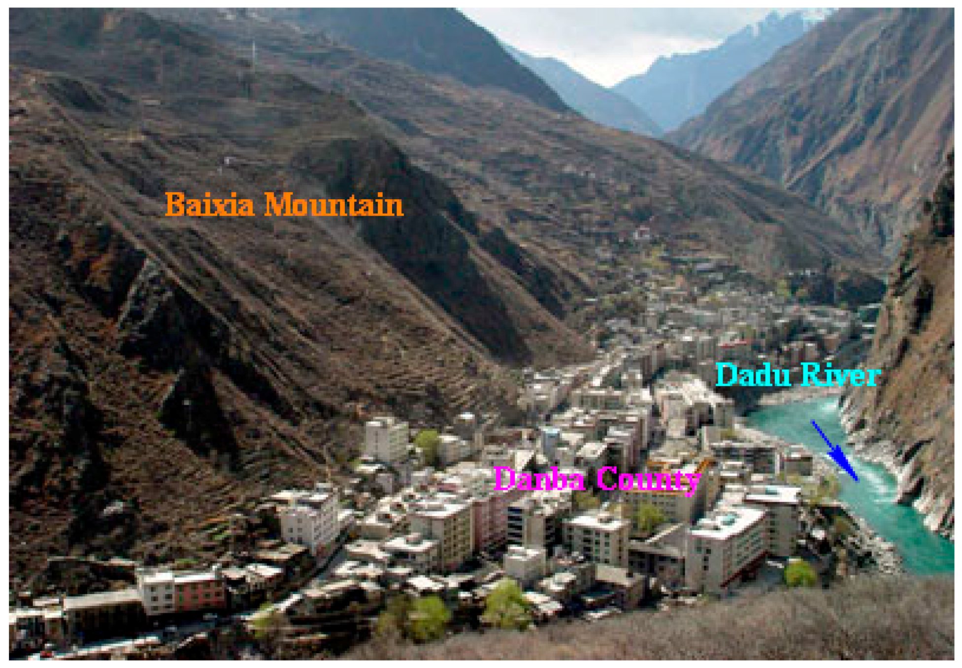
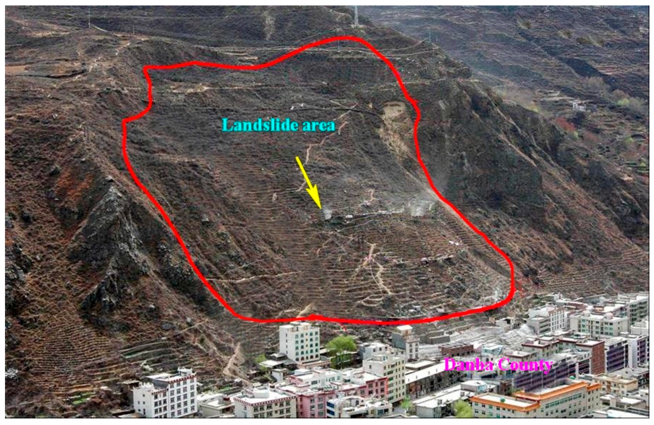
3.1. Basic Characteristics of Landside

The landslide area is located in the alpine and gorge region near the Dadu River in the eastern margin of the Tibetan Plateau. This area is characterized by undulating hills and steep mountains. The landslide is located on the right bank of the Dadu River, namely the high and steep slope at the bottom of Baixia Mountain, which is on the south side of Jianshe Street, Danba County, as shown in Figure 1. This landside is formed and developed on the basis of ancient landsides. It is a massive accumulative landslide. The elevation of its frontend is between 1881 m and 1892 m; the elevation of its back end is between 2070 m and 2110 m. The frontend of the landslide reaches to Jianshe Street at the slope foot. The perimeter of the landside is very clear. The relative altitude of its anterior and posterior edge is 223 m. The widths of its front, middle, and back ends are about 250 m, 230 m and 280 m, respectively. The length of landside is about 290 m, the area is about 0.08 km2, the thickness is 18–45.23 m, the average thickness is about 30 m, and the volume is about 2.2 million m3. According to the investigation and dynamic monitoring of the ground, the deformation of the landslide surface is very obvious, including the tensile crack in the back, the bulging deformation on the front edge, the shear crack on both sides of the landslide, and so on. The displacement of the landslide surface is more than 30 mm/day; the displacement velocity in the middle and front of the landslide is more than 35 mm/day. Cracks in the landslide perimeter are connected. All as shown in Figure 2.

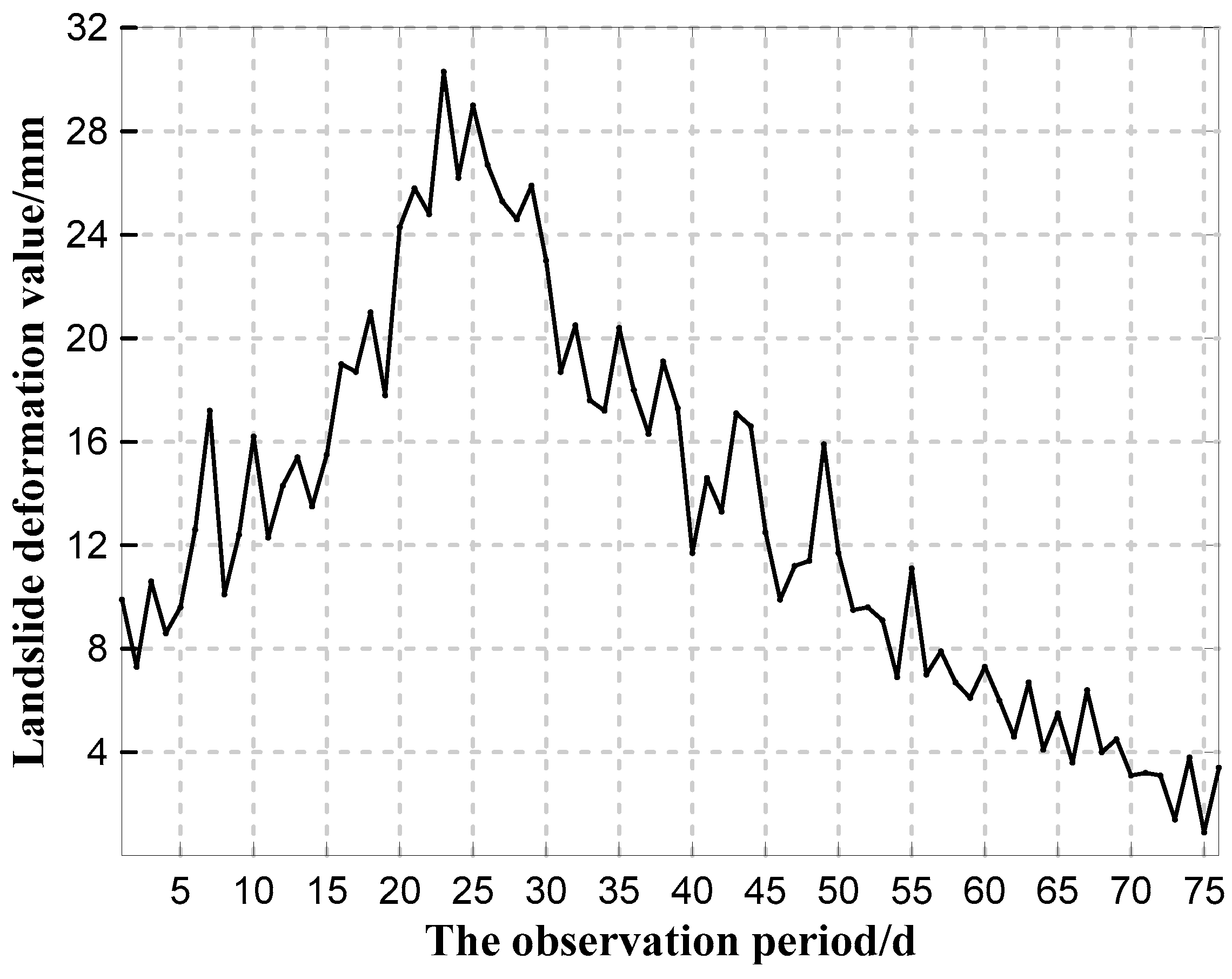
3.2. Experimental Data

In this study, the experimental data are derived from the Danba landslide surface displacement [31]. Considering the Sixth Mirror monitoring points is the key and its monitoring data are relatively complete. Thus, in this paper, the monitoring data of the Sixth Mirror monitoring points are selected to be forecasted and analyzed. There are 76 periods of observation data, as shown in Figure 3.
Figure 3 shows that the landslide deformation was relatively violent, nonlinear, very non-stationary, and random. The magnitude of deformation was relatively large. A sharp convex peak was formed during the rising trend, and it changed into a downward trend. The difference between the maximum and minimum deformation value was 29.4 mm. It has a certain representativeness. Clearly it is very difficult to reflect the trend of landslide deformation if using the traditional forecasting method.

3.3. Modeling Process

To verify the feasibility of the prediction model based on MEEMD, approximate entropy and WLS-SVM, the following 11 types of schemes were established for comparison with each other; Scheme 1 (Wavelet neural network prediction model), Scheme 2 (SVM prediction model), Scheme 3 (LS-SVM prediction model), Scheme 4 (Wavelet neural network prediction model taking the reconstructed phase space of the original sequence as samples), Scheme 5 (LS-SVM prediction model taking the reconstructed phase space of the original sequence as samples), Scheme 6 (Wavelet neural network prediction model taking each new subsequence as a sample), Scheme 7 (Wavelet neural network prediction model taking the reconstructed phase space of the new subsequence as samples), Scheme 8 (LS-SVM prediction model taking each new sequence as a sample), Scheme 9 (LS-SVM model taking the reconstructed phase space of the new subsequence as samples), Scheme 10 (WLS-SVM prediction model taking the new subsequence as samples), and Scheme 11 (the algorithm of this paper). To reduce the modeling error, the landslide deformation data were pre-processed, and the data were normalized to the [−1, 1] interval and reverted to the original interval after using the model to predict. In this paper, the data of the first 56 periods were taken as a training sample, and the data of the last 20 periods were taken as the test sample; the prediction steps were 5, 10, and 20. For example, when the prediction step was 5, the model was established to forecast the 57th to the 61st period data based on the data of the 1st to the 56th period; then the model was established to predict the 62nd to the 66th period data based on the data of the 6th to 61st period and so on, until the data of the 76th period were predicted. The modeling processes in this paper were as follows:
(1)
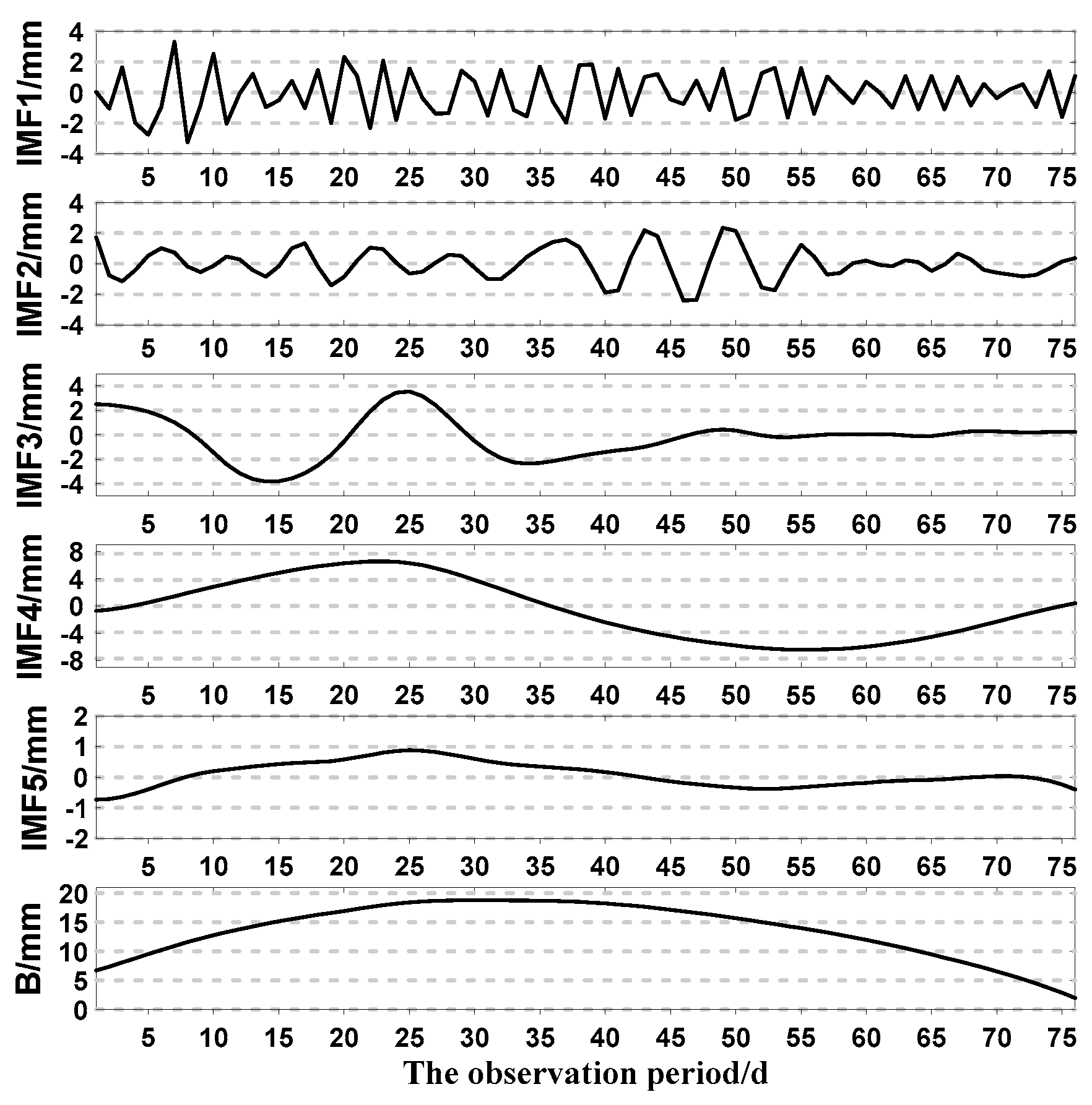
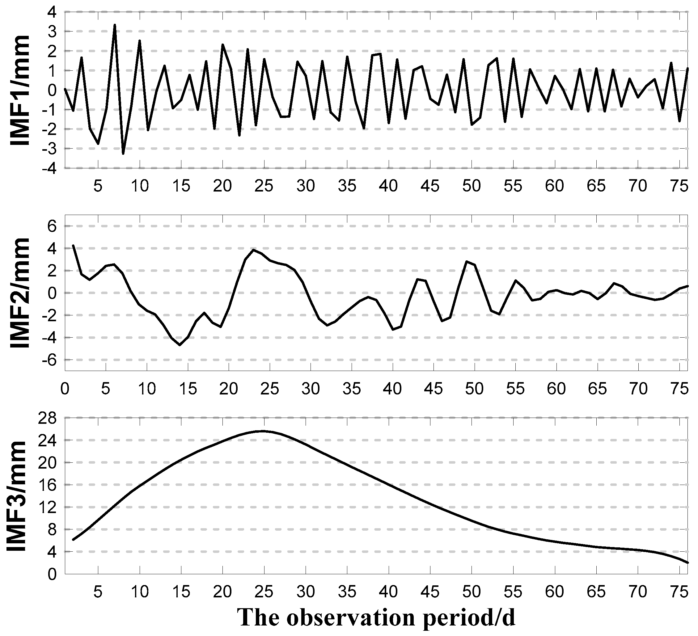
To make the complex sequence smooth, the landslide sequence was decomposed to obtain a finite number of IMF components and a margin using MEEMD.
(2)
Analyzing the complexity of each component using approximate entropy, combining the adjacent components with a small difference in entropy, and obtaining a new subsequence to reduce the size of the calculation.
(3)
Reconstructing the phase space of each new subsequence using the C-C method, which could avoid the random selection of the input dimensions of the prediction model.
(4)
Establishing the WLS-SVM prediction model based on the reconstructed phase space of the new subsequences by Step 3 to make a forecast.
(5)
Superposing the prediction result of each new subsequence to obtain the final forecast value of landslide deformation, and then evaluating the accuracy of each model.

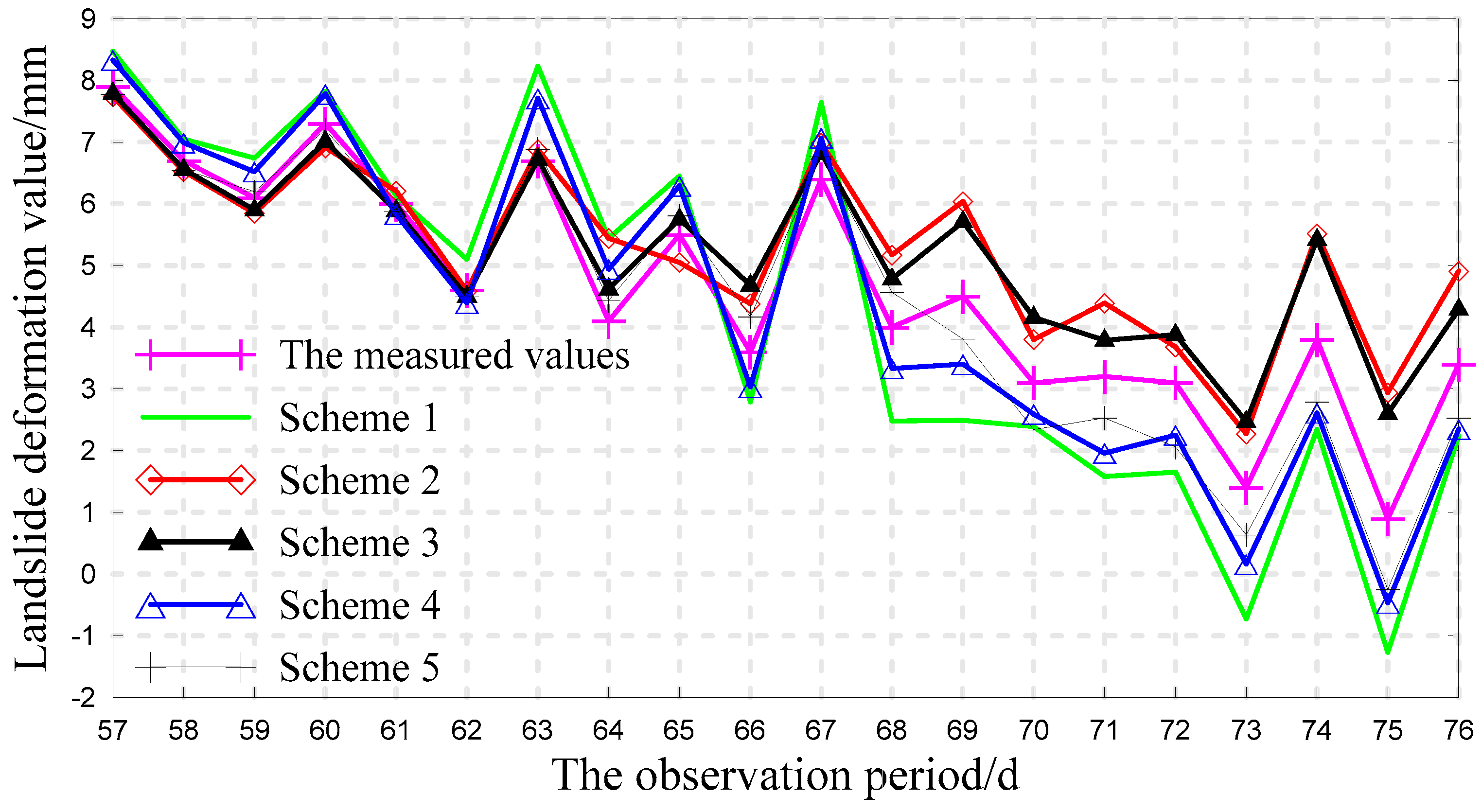
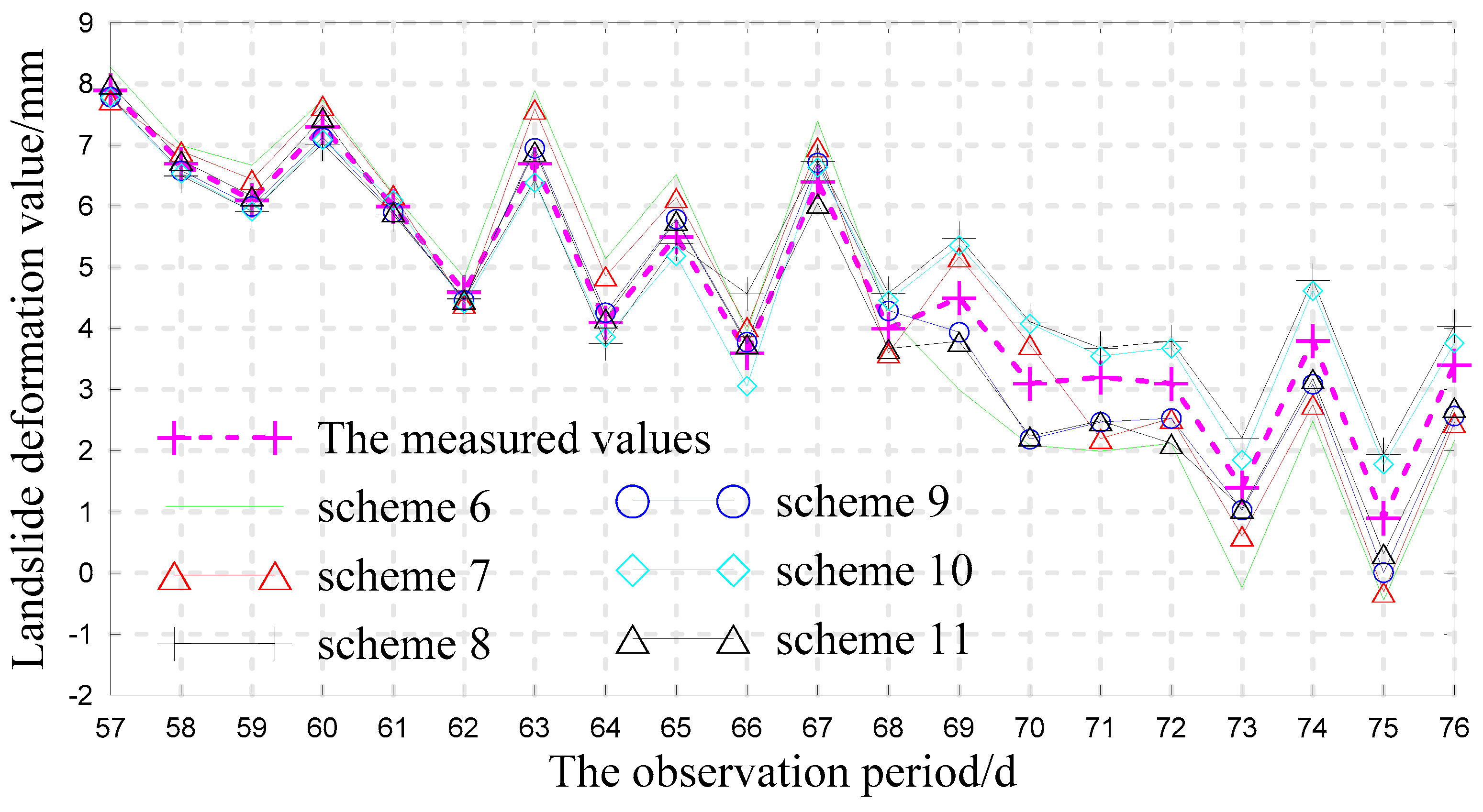
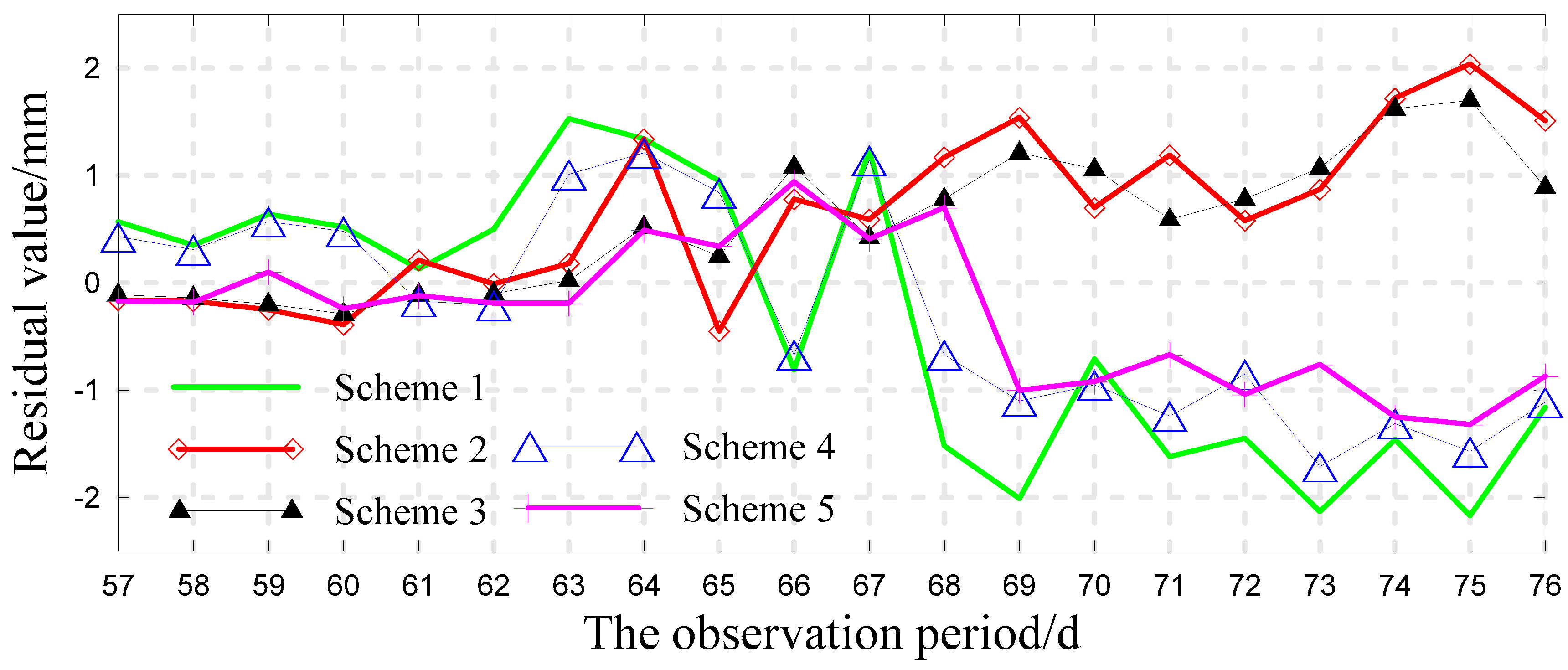
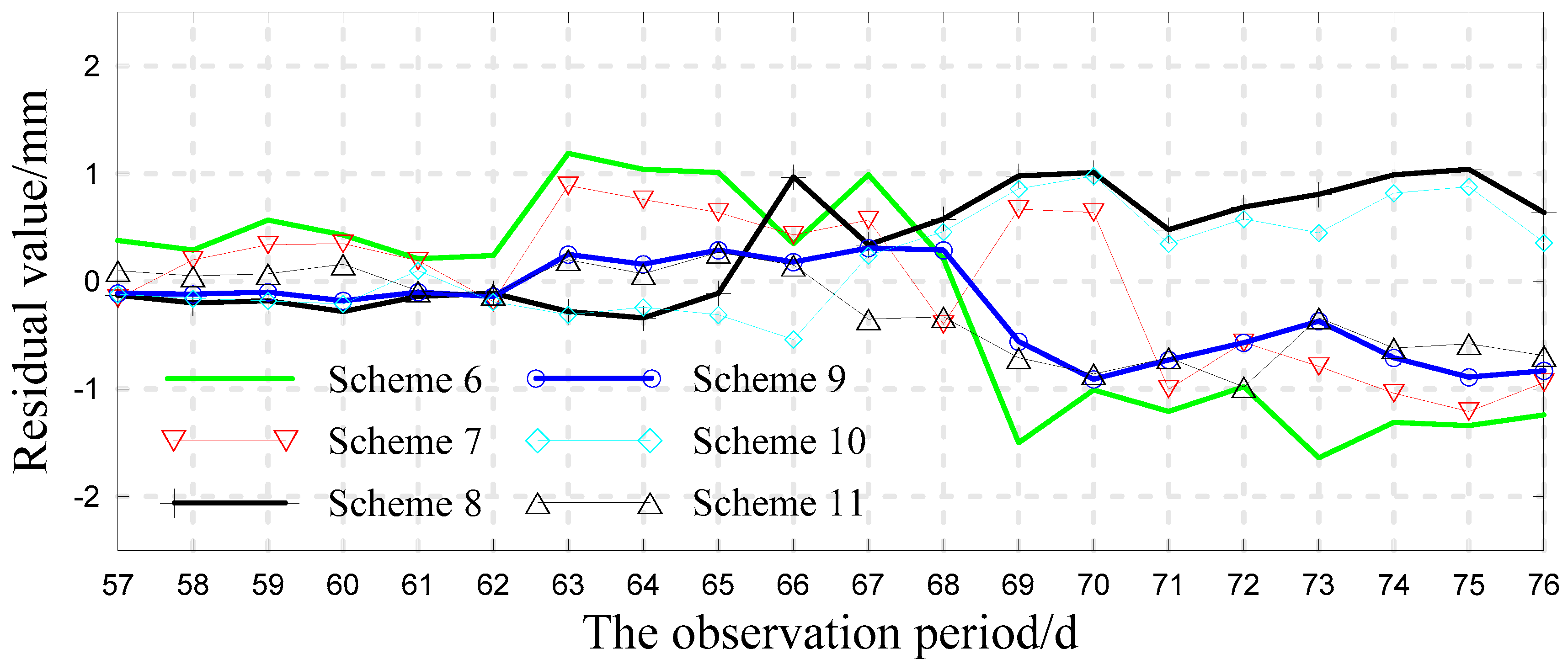
3.4. Analysis of the Forecast Results

From the analysis in Section 3.1, the landslide is relatively complex. To better analyze the chaotic time series of the landslide and to obtain higher prediction accuracy, MEEMD and approximate entropy were used to analyze the landslide sequence. Each component decomposed by MEEMD is shown in Figure 4.
As shown in Figure 4 MEEMD can effectively decompose the time-frequency information of the landslide sequence, and the frequency of each component is gradually decreasing. However, due to the obviously non-stationary, the landslide sequence is decomposed into more components. Directly establishing the prediction model to forecast each component will appreciably increase the amount of modeling required and reduce efficiency. To predict the landslide sequence more effectively, the approximate entropy theory was used to evaluate the complexity of each component. The approximate entropy of each IMF is shown in Figure 5.
As shown in Figure 5, the approximate entropy of each component decreases with the reduction of the component’s frequency, which further illustrates that MEEMD can effectively reduce the non-stationarity of the original sequence, decompose the component step by step with a gradual reduction in complexity, and verify the effectiveness of applying the approximate entropy to the complexity of the landslide sequence. Figure 5 also shows that the differences in the entropies of IMF2, IMF3, IMF4, IMF5, and IMF6 (margin B) are not very large. To reduce the computing scale of the modeling, they are combined and superposed. The results are shown in Table 1, and each new subsequence is shown in Figure 6. From Figure 6; the high-frequency information and strong volatility are fully reflected by IMF1, IMF2 represents a certain randomness of the landslide sequence, and IMF3 more obviously reflects the overall trend of the landslide deformation.
The WLS-SVM was established to make a prediction according to the new subsequences. The optimal input dimension was determined by the reconstructed phase space of each new subsequence. Then the grid search method was used to select the optimal parameters of WLS-SVM to make a forecast. The superposition of each component was the prediction result. At the same time, when the prediction step was set as 5, Schemes 1 to 11 were established for comparison and analysis. The prediction results of Schemes 1 to 5 are shown in Figure 7, and the prediction results of Schemes 6 to 11 are shown in Figure 8. Figure 9 and Figure 10 show the residuals of the corresponding models.
As shown in Figure 7 and Figure 8, the prediction results from the 57th period to the 67th period of the 11 schemes are relatively good. For the 68th period to the 76th period, the prediction results of Schemes 4 and 5, which used phase space to reconstruct the original sequence for modeling and forecasting, are better than those of Schemes 1 to 3. The prediction results of Schemes 6 to 11, which used a new subsequence combined by MEEMD and approximate entropy as sample data, are also relatively good. Comparison of Scheme 6, 8, and 10 reveals that the prediction result of SVM is more stable than those of the neural network. From Schemes 7, 9, and 11, the prediction effect by using phase space to reconstruct each new subsequence is better than other schemes. The prediction values of Schemes 9 and 11 are in good agreement with the actual values.
As further shown in Figure 9 and Figure 10, the prediction error of Schemes 1 to 3 is relatively large and clearly outstanding in some of the prediction periods. In addition, the prediction error increases with the extension of forecast time. Clearly it is not easy to achieve satisfactory prediction results directly using a single model. Comparison of Schemes 1, 4, 6, and 7 reveals that the prediction result of the wavelet neural network is very unstable, and the fluctuation of its prediction error is relatively large, which further demonstrates the disadvantages of the neural network itself. As shown in Schemes 4 and 5, reconstructing the phase space of the original sequence has a certain effect on improving the prediction accuracy of the LS-SVM model. However from the 68th period to the 76th period, the prediction error of Scheme 5 also becomes relatively large with the increase in the forecast period. Thus, because of the mutual interference among different characteristic information, direct modeling through raw data reconstruction can make it difficult for the model to accurately reflect the evolution law of the landslide, and it is not conducive to a long-term prediction. The prediction error of Schemes 8 to 11, which merged similar information using MEEMD and approximate entropy, has very good stability. Moreover the forecast results of Scheme 9 and Scheme 11, which used phase space reconstruction theory to select the optimal input dimension of the model, are more stable than those of other schemes, and the change in the error curve is also relatively steady. Comparatively the forecast result of Scheme 11 is slightly better than that of Scheme 9. Thus the landslide sequence processed by MEEMD and approximate entropy can make the model truly reflect the deformation rules and obtain a good prediction result. Reconstructing the sample data of the model by using phase space reconstruction theory can avoid the randomness of the model input dimension, effectively improve the model's performance, and further enhance the prediction accuracy of the model.
To further evaluate the model performance, the internal accordant accuracy (IAA), external accordant accuracy (EAA) and running time in the training and testing of each scheme in each prediction step (step 5, for example) were compared and analyzed. The results are shown in Table 2.
From Table 2, when the original data are directly used for modeling, both the training error and the prediction error of the model are relatively large and the error increases rapidly. Through sample data analysis of the new landslide sequence processed by MEEMD and approximate entropy, for a relatively high-frequency and a strong volatility of the IMF1 new subsequence, the training error and testing error of Schemes 6 to 11 are almost the same. Through comparison of the three new subsequences of IMF1, IMF 2, and IMF3, it can be found that the training and prediction error of the first 5 steps of each scheme are not quite different with the decrease of the frequency of each component, and the training and testing error of each scheme are increased in varying degrees with the increase in the forecast period. From Schemes 6 and 7, the error increment of neural network model is the largest. Comparison of Schemes 8 to 11 reveals that selecting the optimal input dimension of the model using phase space reconstruction theory is helpful for reducing the model training and testing error, and the extent of the error increase is small. Comparison of Schemes 9 and 10 reveals that the improved LS-SVM is better than the traditional LS-SVM. Therefore the robustness of SVM plays a certain role in improving the model performance. From the running time of each scheme, less time is used for establishing a single prediction model using the original data directly. Compared with each component, under the same conditions, the time used for each component prediction is less than that from using the original data directly. The running time of the model is increased with the increase in the complexity of the combined model. For the same model, the training and prediction time of each component is less than that from directly using the original data. When training and forecasting for each component, the running time for the same model is increased with the decrease of the component’s frequency. Comparison between Schemes 8 and 10 and Schemes 9 and 11 reveals that the performance of the improved LS-SVM model is better than that of the traditional LS-SVM model. Clearly the running time of the model is related to the complexity of the sample data and the performance of the combined model. Therefore the algorithm in this paper is feasible through comprehensive consideration of the accuracy and running time of the model.
To further explore the effectiveness of each scheme for different prediction steps, Schemes 1 to 11 were established with steps 5, 10, and 20. Additionally the minimum/maximum, RMSE, and mean absolute error (MAE) were used to analyze the model precision, as shown in Table 3. The prediction accuracy of each of the predicting methods has a different degree of change with the increase in the prediction step. The prediction accuracy of Schemes 1, 2, and 3 decreases significantly. The prediction accuracy of Schemes 8 to 11 are much better than those of other schemes, and the extents of error increase are relatively small; the prediction accuracy of Scheme 11 is the best among Schemes 8 to 11. From the minimum and maximum residual value, Scheme 11 can better control the minimum and maximum residual values and effectively reduce the error interval. In conclusion, this algorithm can not only guarantee good local prediction values, but it also has preferable global prediction accuracy. Therefore the algorithm can obtain a better prediction result when the landslide deformation is complex or in long-term prediction.

4. Conclusions

For a landslide with a complex deformation, it is difficult to directly establish an effective model for analysis, and it is not conducive to long-term prediction. In this paper, a combination prediction algorithm based on MEEMD, approximate entropy, and WLS-SVM was proposed. The theoretical analysis and calculation examples indicate that MEEMD can retain the real signals, effectively separate the implicit time-frequency information in the landslide deformation sequence, and reduce the mutual interference of information associated with different features. Approximate entropy can effectively analyze the complexity of the landslide sequence. The new subsequences with distinct complexity are obtained by reconstructing each component based on entropy values. They can better reflect the different time-frequency information of landslide chaotic sequences, and they can reduce the computing scale at the same time. The selection of optimal model parameters by using chaotic phase space reconstruction theory and the grid search method can effectively improve the prediction precision. The algorithm in this paper can well express and reflect landslide deformation characteristics, effectively control the extreme residual values, and reduce the error interval. This algorithm can not only improve the global prediction accuracy of landslide deformation, but it can also ensure good local prediction accuracy. The algorithm can describe well the characteristics of the complex chaotic system, which provides a new way to improve the prediction accuracy of landslide deformation. Since the algorithm in this paper combines the performance of multiple methods, it will increase the complexity and running time of the model to a certain extent. The question of how to further improve the running speed and performance of the combined model is the next step to be studied.

Acknowledgments

This work was supported by the National Natural Science Foundation of China (41461089, 41664002) and Guangxi Natural Science Foundation of China (2015GXNSFAA139230).

Author Contributions

Shaofeng Xie conceived and designed the experiments and performed the modeling; Yueji Liang gave relevant technical support and finished the first draft; Zhongtian Zheng and Haifeng Liu analyzed the data and reviewed and edited the draft. All authors discussed the basic structure of the manuscript and read and approved the manuscript.

Conflicts of Interest

The authors declare no conflict of interest.

References

  1. Behling, R.; Roessner, S.; Kaufmann, H.; Kleinschmit, B. Automated spatiotemporal landslide mapping over large areas using rapideye time series data. Remote Sens. 2014, 6, 8026–8055. [Google Scholar] [CrossRef]
  2. Dou, J.; Yamagishi, H.; Pourghasemi, H.R.; Yunus, A.P.; Song, X.; Xu, Y.; Zhu, Z. An integrated artificial neural network model for the landslide susceptibility assessment of Osado Island, Japan. Nat. Hazards 2015, 78, 1749–1776. [Google Scholar] [CrossRef]
  3. Zhou, S.; Chen, G.; Fang, L. Distribution pattern of landslides triggered by the 2014 Ludian earthquake of China: Implications for regional threshold topography and the seismogenic fault identification. ISPRS Int. J. Geo-Inf. 2016, 5, 46. [Google Scholar] [CrossRef]
  4. Manfré, L.A.; de Albuquerque Nóbrega, R.A.; Quintanilha, J.A. Evaluation of multiple classifier systems for landslide identification in Landsat Thematic Mapper (TM) images. ISPRS Int. J. Geo-Inf. 2016, 5, 164. [Google Scholar] [CrossRef]
  5. Chen, W.; Li, X.; Wang, Y.; Chen, G.; Liu, S. Forested landslide detection using LiDAR data and the random forest algorithm: A case study of the Three Gorges. Remote Sens. Environ. 2014, 152, 291–301. [Google Scholar] [CrossRef]
  6. Li, Z.; Jiao, Q.; Liu, L.; Tang, H.; Liu, T. Monitoring geologic hazards and vegetation recovery in the Wenchuan earthquake region using aerial photography. ISPRS Int. J. Geo-Inf. 2014, 3, 368–390. [Google Scholar] [CrossRef]
  7. Akcay, O. Landslide fissure inference assessment by ANFIS and logistic regression using UAS-based photogrammetry. ISPRS Int. J. Geo-Inf. 2015, 4, 2131–2158. [Google Scholar] [CrossRef]
  8. Stumpf, A.; Malet, J.P.; Allemand, P.; Pierrot-Deseilligny, M.; Skupinski, G. Ground-based multi-view photogrammetry for the monitoring of landslide deformation and erosion. Geomorphology 2015, 231, 130–145. [Google Scholar] [CrossRef]
  9. Ballabio, C.; Sterlacchini, S. Support vector machines for landslide susceptibility mapping: The Staffora River Basin case study, Italy. Math. Geosci. 2012, 44, 47–70. [Google Scholar] [CrossRef]
  10. Cortes, C.; Vapnik, V. Support vector networks. Mach. Learn. 1995, 20, 273–297. [Google Scholar] [CrossRef]
  11. Zhao, H. The application of support vector machine in the deformation prediction of tunnel surrounding rock. Chin. J. Rock Mech. Eng. 2005, 24, 649–652. (In Chinese) [Google Scholar]
  12. Suykens, J.A.K.; Brabanter, J.D.; Lukas, L.; Vandewalle, J. Weighted least squares support vector machines: Robustness and sparse approximation. Neurocomputing 2002, 48, 85–105. [Google Scholar] [CrossRef]
  13. Shi, J.; Liu, X. Melt index prediction by weighted least squares support vector machines. J. Appl. Polym. Sci. 2006, 101, 285–289. [Google Scholar] [CrossRef]
  14. Qin, S.; Jiao, J.J.; Wang, S. A nonlinear dynamical model of landslide evolution. Geomorphology 2002, 43, 77–85. [Google Scholar] [CrossRef]
  15. Qin, S.Q.; Jiao, J.J.; Wang, S.J. The predictable time scale of landslides. Bull. Eng. Geol. Environ. 2001, 59, 307–312. [Google Scholar] [CrossRef]
  16. Huang, Z.; Law, K.T.; Liu, H.; Jiang, T. The chaotic characteristics of landslide evolution: A case study of Xintan landslide. Environ. Geol. 2009, 56, 1585–1591. [Google Scholar] [CrossRef]
  17. Hovius, N.; Stark, C.P.; Tutton, M.A.; Abbott, L.D. Landslide-driven drainage network evolution in a presteady state mountain belt: Finisterre Mountains, Papua New Guinea. Geology 1998, 26, 1071–1074. [Google Scholar] [CrossRef]
  18. Wang, X.; Fan, Q.; Xu, C.; Li, Z. Dam deformation predictions based on wavelet transforms and support vector machine. Geomat. Inf. Sci. Wuhan Univ. 2008, 33, 469–471. (In Chinese) [Google Scholar]
  19. Li, X.; Xu, J. Landslide deformation prediction based on the wavelet analysis and LSSVM. J. Geod. Geodyn. 2009, 29, 127–130. (In Chinese) [Google Scholar]
  20. Lian, C.; Zeng, Z.; Yao, W.; Tang, H. Displacement prediction model of landslide based on a modified ensemble empirical mode decomposition and extreme learning machine. Nat. Hazards 2013, 66, 759–771. [Google Scholar] [CrossRef]
  21. Shen, Z.; Wang, Q.; Shen, Y.; Jin, J.; Lin, Y. Accent extraction of emotional speech based on modified ensemble empirical mode decomposition. In Proceedings of the 2010 IEEE Instrumentation & Measurement Technology Conference (I2MTC), Austin, TX, USA, 3–6 May 2010.
  22. Wu, Z.; Huang, N.E.; Chen, X. The multi-dimensional ensemble empirical mode decomposition method. Adv. Adapt. Data Anal. Theory Appl. 2009, 1, 339–372. [Google Scholar] [CrossRef]
  23. Pincus, S.M. Approximate entropy as a measure of system complexity. Proc. Natl. Acad. Sci. USA 1991, 88, 2297–2301. [Google Scholar] [CrossRef] [PubMed]
  24. Richman, J.S.; Moorman, J.R. Physiological time-series analysis using approximate entropy and sample entropy. Am. J. Physiol. Heart Circ. Physiol. 2000, 278, 2039–2049. [Google Scholar]
  25. Kennel, M.B.; Brown, R.; Abarbanel, H.D.I. Determining embedding dimension for phase space reconstruction using a geometrical construction. Phys. Rev. A 1992, 45, 3403–3411. [Google Scholar] [CrossRef] [PubMed]
  26. Liu, X.; Jia, D.; Li, H.; Jiang, J. Research on kernel parameter optimization of support vector machine in speaker recognition. Sci. Technol. Energy 2010, 10, 1669–1673. (In Chinese) [Google Scholar]
  27. Monfared, M.; Rastegar, H.; Kojabadi, H.M. A new strategy for wind speed forecasting using artificial intelligent methods. Renew. Energy 2009, 34, 845–848. [Google Scholar] [CrossRef]
  28. Wu, Z.; Huang, N.E. Ensemble empirical mode decomposition: A noise assisted data analysis method. Adv. Adapt. Data Anal. 2009, 1, 1–41. [Google Scholar] [CrossRef]
  29. Zhang, J.; Yan, R.; Gao, R.X.; Feng, Z. Performance enhancement of ensemble empirical mode decomposition. Mech. Syst. Signal Process. 2010, 24, 2104–2123. [Google Scholar] [CrossRef]
  30. Takens, F. Detecting Strange Attractors in Turbulence; Dynamical Systems and Turbulence, Lecture Notes in Mathematics; Springer: Berlin, Germany, 1981. [Google Scholar]
  31. Li, L. Landslide Prediction Research Based on the Theory of Phase Space Reconstruction; Chengdu University of Technology: Chengdu, China, 2008. (In Chinese) [Google Scholar]
Figure 1. The location map of the Danba landside.
Ijgi 06 00005 g001
Figure 2. The scope of the Danba landslide.
Ijgi 06 00005 g002
Figure 3. The deformation sequence of landslide displacement.
Ijgi 06 00005 g003
Figure 4. The decomposition results of MEEMD.
Ijgi 06 00005 g004
Figure 5. The approximate entropy of each component.
Ijgi 06 00005 g005
Figure 6. New subsequence.
Ijgi 06 00005 g006
Figure 7. Prediction results of Schemes 1 to 5.
Ijgi 06 00005 g007
Figure 8. Prediction results of Schemes 6 to 11.
Ijgi 06 00005 g008
Figure 9. Prediction errors of Schemes 1 to 5.
Ijgi 06 00005 g009
Figure 10. Prediction errors of Schemes 6 to 11.
Ijgi 06 00005 g010
Table 1. The combined results of each component.
Intrinsic Mode FunctionComponent Serial Number
New IMFIMF1IMF2IMF3
Original IMFIMF1IMF2,IMF3IMF4,IMF5,IMF6
Table 2. Statistics of residual sequences (unit: mm).
SamplePrediction ModelStep Size: 1 to 5Step Size: 6 to 10Step Size: 11 to 15Step Size: 16 to 20Running Time/s
IAAEAAIAAEAAIAAEAAIAAEAA
Original dataScheme 1±0.44±0.53±0.95±1.22±1.34±1.66±1.52±1.9313.92
Scheme 2±0.20±0.28±0.61±0.81±1.11±1.22±1.32±1.6210.27
Scheme 3±0.13±0.20±0.50±0.61±0.84±0.96±1.24±1.428.13
Scheme 4±0.39±0.47±0.84±0.96±0.99±1.16±1.37±1.5017.35
Scheme 5±0.13±0.19±0.48±0.57±0.75±0.86±1.09±1.2011.97
IMF1Scheme 6±0.09±0.13±0.11±0.15±0.15±0.19±0.20±0.2311.42
Scheme 7±0.06±0.10±0.10±0.14±0.13±0.17±0.16±0.2014.84
Scheme 8±0.03±0.08±0.06±0.10±0.10±0.16±0.13±0.187.51
Scheme 9±0.03±0.07±0.03±0.08±0.09±0.13±0.10±0.159.14
Scheme 10±0.03±0.07±0.04±0.09±0.08±0.13±0.10±0.155.84
Scheme 11±0.00±0.05±0.03±0.08±0.05±0.11±0.08±0.147.92
IMF2Scheme 6±0.19±0.24±0.47±0.54±0.89±1.06±1.10±1.2112.67
Scheme 7±0.16±0.20±0.36±0.41±0.60±0.68±0.67±0.7616.79
Scheme 8±0.10±0.15±0.21±0.27±0.35±0.41±0.39±0.487.94
Scheme 9±0.09±0.13±0.13±0.18±0.27±0.33±0.36±0.4110.97
Scheme 10±0.10±0.14±0.18±0.24±0.29±0.37±0.38±0.456.96
Scheme 11±0.07±0.11±0.06±0.10±0.19±0.28±0.29±0.378.27
IMF3Scheme 6±0.31±0.38±0.56±0.64±1.01±1.19±1.15±1.3013.57
Scheme 7±0.21±0.26±0.37±0.43±0.79±0.85±0.90±0.9716.91
Scheme 8±0.17±0.22±0.28±0.34±0.59±0.67±0.61±0.698.10
Scheme 9±0.13±0.18±0.15±0.21±0.45±0.51±0.47±0.5611.37
Scheme 10±0.16±0.20±0.23±0.29±0.55±0.61±0.57±0.647.24
Scheme 11±0.11±0.18±0.11±0.19±0.44±0.51±0.46±0.539.14
Table 3. The contrast of each scheme’s accuracy with different prediction steps (unit: mm).
ModelPrediction Step: 5Prediction Step: 10Prediction Step: 20
MaxMinRMSEMAEMaxMinRMSEMAEMaxMinRMSEMAE
Scheme 1−2.170.131.2831.141−2.310.341.3121.273−3.110.271.4821.395
Scheme 22.04−0.160.9860.7931.980.151.1410.9042.140.571.2071.016
Scheme 31.70−0.100.8200.6471.67−0.240.9560.7411.990.341.1890.861
Scheme 4−1.71−0.170.9740.878−1.83−0.341.0850.957−2.010.471.2611.204
Scheme 5−1.320.100.7110.595−1.180.210.8540.611−1.570.291.0970.773
Scheme 6−1.340.210.9730.857−1.570.181.0370.911−1.61−0.171.1970.999
Scheme 7−1.21−0.160.6730.599−1.390.090.7940.715−1.45−0.270.8970.809
Scheme 81.04−0.110.6170.5151.21−0.100.6980.6011.28−0.090.7880.689
Scheme 9−0.91−0.100.4800.390−0.95−0.100.4920.397−1.000.070.5040.407
Scheme 100.980.100.4960.4170.89−0.130.5790.4970.95−0.090.6570.479
Scheme 11−0.860.050.4720.373−0.880.010.4840.3800.91−0.040.4950.397

