A Spatial Lattice Model Applied for Meteorological Visualization and Analysis

Abstract

Meteorological information has obvious spatial-temporal characteristics. Although it is meaningful to employ a geographic information system (GIS) to visualize and analyze the meteorological information for better identification and forecasting of meteorological weather so as to reduce the meteorological disaster loss, modeling meteorological information based on a GIS is still difficult because meteorological elements generally have no stable shape or clear boundary. To date, there are still few GIS models that can satisfy the requirements of both meteorological visualization and analysis. In this article, a spatial lattice model based on sampling particles is proposed to support both the representation and analysis of meteorological information. In this model, a spatial sampling particle is regarded as the basic element that contains the meteorological information, and the location where the particle is placed with the time mark. The location information is generally represented using a point. As these points can be extended to a surface in two dimensions and a voxel in three dimensions, if these surfaces and voxels can occupy a certain space, then this space can be represented using these spatial sampling particles with their point locations and meteorological information. In this case, the full meteorological space can then be represented by arranging numerous particles with their point locations in a certain structure and resolution, i.e., the spatial lattice model, and extended at a higher resolution when necessary. For practical use, the meteorological space is logically classified into three types of spaces, namely the projection surface space, curved surface space, and stereoscopic space, and application-oriented spatial lattice models with different organization forms of spatial sampling particles are designed to support the representation, inquiry, and analysis of meteorological information within the three types of surfaces. Cases studies are conducted by (1) performing a visualization of radar data that is used to describe the reflectivity factor of a raindrop and the pressure field information acquired from the National Centers for Environmental Prediction (NCEP), and (2) taking cutting analysis as another example where advanced meteorological analysis is performed. The results show that the proposed spatial lattice model can contribute to the feasible and effective analysis of meteorological information.

1. Introduction

People have suffered greatly from meteorological disasters in the past, and the losses from meteorological disasters can be reduced by early warnings based on an analysis of the meteorological information that contains obvious spatial-temporal characteristics. Thus, it is meaningful to employ geographic information system (GIS) to visualize and analyze the meteorological information, and using a geographic information system to support meteorological applications has become a hot topic [1]. Achievements have been made in recent years. GIS was used as an infrastructure tool at the National Center for Atmospheric Research (NCAR) to address spatial data management, interoperability, and geoinformatics issues in the atmospheric sciences in 2005 [2]. A visual GIS tool was developed to explore new uncertainties of numerical weather models [3]. Various web-based visualization systems to support the expression of global change and climatic distribution patterns [4,5,6]. Using GIS, the annual runoff and climate change in eastern Ontario and southwestern Quebec was analyzed [7]. Although the above-mentioned studies have enhanced the traditional research strategies in meteorological fields in a broader way, an important limiting factor is that a suitable data model is urgently needed [8]. In particular, there is still a lack of multi-dimensional data models that can be used to re-build the meteorological space with an unstable shape and fuzzy boundary. Thus, the current GIS still has limited capacities to satisfy both the representation and analysis demands in the meteorological field. Much work is still needed to employ the current GIS and its data models to represent climatic phenomena accurately and to conduct dynamic diagnosis, which will play significant roles in future meteorological research [9].

A data model is an important tool that bridges the real world with the computer world, and it is also the foundation of expressing and analyzing geo-spatial information with a GIS [10]. During recent decades, a series of relevant data models were proposed. In summary, there are surface models, e.g., the boundary-represented (B-rep) model and the mesh surface model, that are used to express objects with their surface boundaries [11]; voxel models, e.g., the tetrahedral model and the triangular prism models, that are used to express solid objects with finitely partitioned volumetric units [12,13,14]; and integrated models that combine surface and voxel models together to describe both the surface and internal structure of these geographic objects [15]. With the above models, geographical information concerning space and objects can be described from different perspectives, and they have thus made a considerable contribution to the development of current GISs. However, meteorological space is a special type of geo-space with fuzziness and uncertainty, and meteorological elements normally have no stable shape and clear boundary. Moreover, this type of meteorological field is changing continually as time passes. It is difficult for researchers employing traditional GIS modeling methods to express dynamic meteorological elements and phenomena, thus limiting the ability of GISs to serve as professional meteorological representations and further meteorological analysis.

In this article, based on an analysis of the meteorological space and meteorological elements, as well as the application requirements in meteorological research, a meteorological spatial modeling method is proposed using a multi-dimensional spatial lattice. It aims to provide an effective carrier for the representation of meteorological information to establish a basis for dynamic meteorological analysis and simulation. The remainder of this article is structured as follows. The basic idea and the logical meteorological spatial lattice model are introduced in Section 2. In Section 3, application-oriented practical spatial lattice models are designed based on commonly used meteorological spaces. Implementation strategies related to the proposed spatial lattice model and advanced analysis are illustrated in Section 4. Related experiments are described in Section 5, and the conclusions and a discussion of directions for further study are finally presented in Section 6.

2. The Basic Idea of the Spatial Lattice Model for Meteorological Analysis

It is well known that meteorological elements normally exist without fixed shapes and are always changing with time. Although they cannot be perceived by human eyes, they fill up the meteorological space in their own way. How to represent the invisible meteorological information performance analysis is still a problem. The basic idea of the spatial lattice model in this article is proposed based on the following hypothesis. Similar to sensors, imagine that there are spatial particles that can detect meteorological information (e.g., temperature and wind speed) around their locations. It may be conceivable that the whole meteorological space is full of such innumerable particles. According to the above hypothesis, by gathering these particles and acquiring information from their inherent properties, the features of the distribution of the meteorological information can be described. In this study, these particles are titled spatial sampling particles of meteorological information, and the basic idea of the meteorological spatial lattice model is proposed as follows: each spatial sampling particle has its own coordinates (x, y, z) and stores the meteorological information in the exact location at a certain time. The meteorological information stored in a particle could be conventional information, such as the temperature, pressure, humidity, wind direction, and wind velocity, but could also be information on the various types of meteorological parameters collected by remote sensing devices (such as radar and satellites) at that location. A spatial sampling particle in meteorological space could be expressed by Equation (1):

$$\mathrm{SP}=F\left(x,y,z,t,P_i\right)$$

(1)

where x, y and z are the location coordinates, t is the time mark, and P_i is the meteorological properties (i $\in$ [1,n]).

In this study, for a specific sampling particle A₀, the position (x₀, y₀, z₀) is constant, and t is a specified value, t₀. This particle will store the meteorological information at time t₀ and in the location (x₀, y₀, z₀). In particular, for parameter P_i, when i = 1, there is only one type of meteorological information stored in this particle; when i > 1, the particle can be used to express multiple types of meteorological information. In this way, along with variations in the different parameters, from an extreme perspective, when these particles fill up the meteorological space very densely, the information they carry will approximately represent the meteorological content in the space. Therefore, through the effective integration, organization, and processing of these particles, the meteorological space filled up with meteorological elements can be expressed and analyzed in a flexible manner.

Based on the spatial sampling particles, the logical spatial lattice model of the meteorological space is explained using Equation (2),

$$\mathrm{SLM}=F\left(S{P}_i,R,FM\right)$$

(2)

where $S{P}_i$ is a spatial sampling particle with both spatial and meteorological information; R is the distribution rule for the sampling particles in the space which controls the shape of the spatial lattice, and is flexible enough to follow the original structures of meteorological data in different applications; and filling model (FM) hints at the mode that these sampling particles fill up and represent the space around them, which can be divided into the point-expansion mode and the point-link mode.

Clearly, in this model, the fundamental unit that carries the meteorological information is the spatial sampling particle, and its location can be regarded as a point in space. A point is the most fundamental geometric object (as shown in Figure 1). On the one hand, it is the basic geometric element that constitutes other complex geometry objects, using the link mode (one type of FM). For example, two points linked together can constitute a line segment, while several points spatially combined together can constitute a patch or a volume. On the other hand, from the perspective of recognition, any object in space can be viewed as a point at a certain scale, and a point itself can also be considered as a dialectical spatial element. Conversely, a point can be one-dimensionally expanded to a line segment, two-dimensionally expanded to a surface, and three-dimensionally expanded to a voxel using the expansion mode (another type of FM). For example, a space (2D or 3D) can be split into different segments, and each segment can be represented using the above expanded results. Similarly, the meteorological space can be presented by spatial sampling particles with their location points. The attached meteorological information in one spatial sampling particle can be used to describe the information in the corresponding expanded cell and, finally, the information of the full meteorological space can be acquired approximately. In this case, the proposed spatial lattice model can express the meteorological elements and phenomena in various forms according to the scale and distribution rule.

3. Application-Oriented Abstraction of 3D Meteorological Space and the Corresponding Spatial Lattice Models

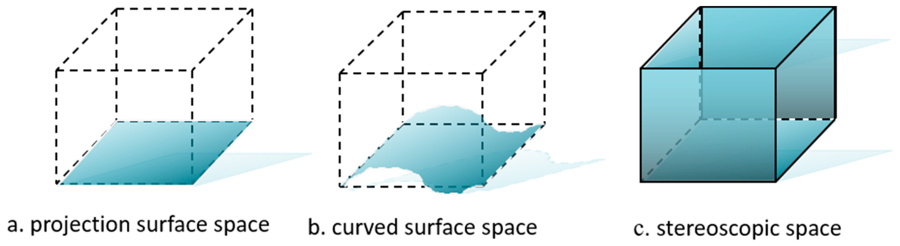
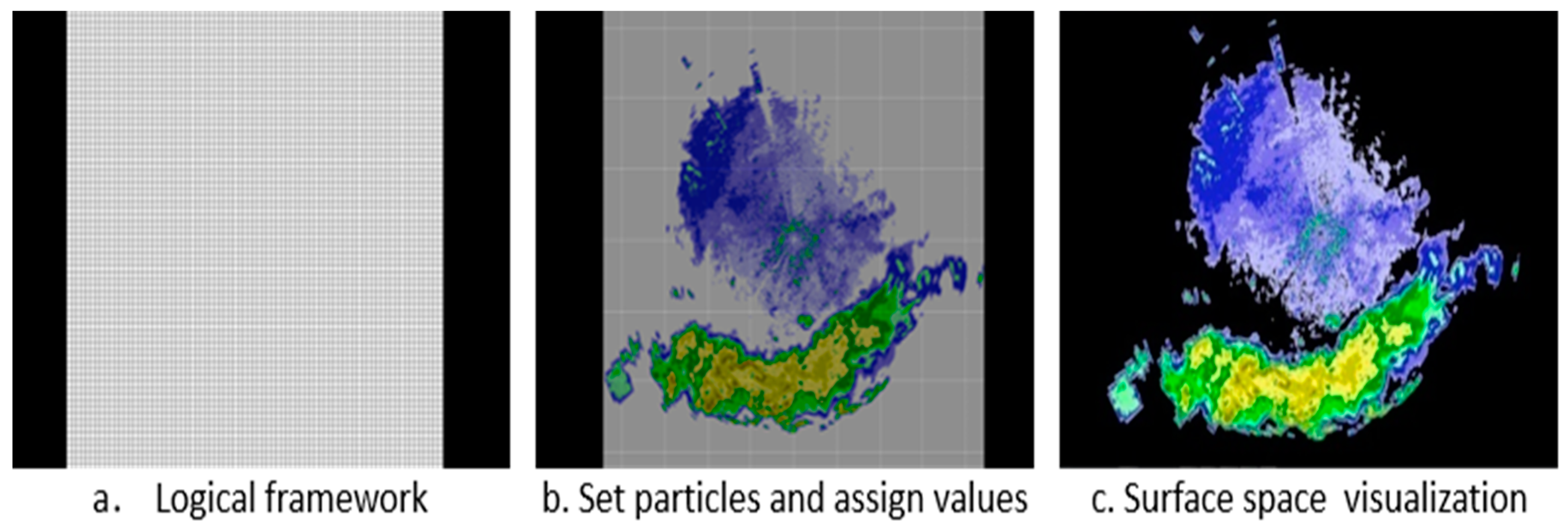
In this study, for practical use, the meteorological space is logically classified into three types of spaces, namely the projection surface space, curved surface space, and stereoscopic space (Figure 2). The stereoscopic space is the closest to reality, while the projection surface space and the curved surface space are the two other abstract forms of meteorological space used to satisfy application customs to conduct visual analysis based on surfaces and layers in the meteorological field.

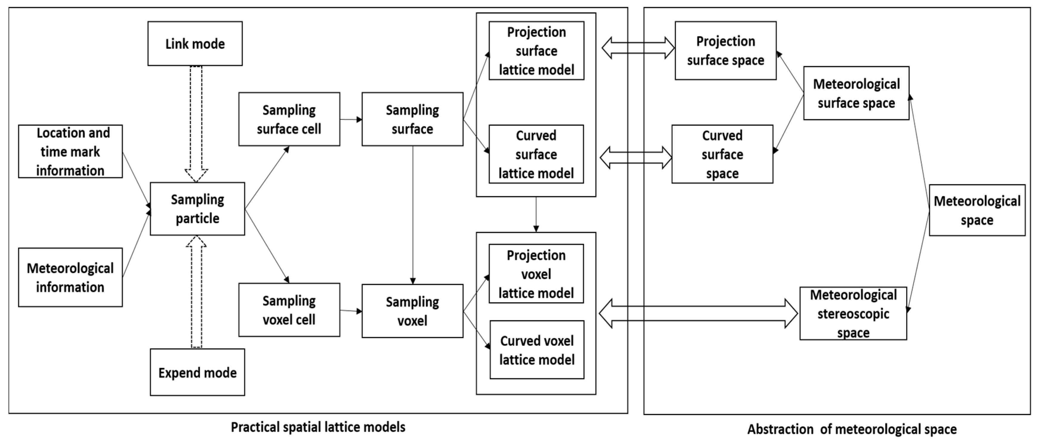
Based on this abstraction, the corresponding practical spatial lattice models can be designed as in Figure 3. In this article, to simplify the explanation, the spatial sampling particles that are used to fill up the abstract meteorological spaces are organized in rows and columns with fixed intervals. It is worth mentioning that although this type of organization can be more compatible with the current meteorological grid data, it is not always necessary to always organize these spatial sampling particles in this regular way. For meteorological spaces with an unclear boundary or that fall within a limited space, the spatial sampling particles can be organized using different distribution rules, and even spatial sampling particles in different parts of the space can employ different distribution rules (R). Together with a corresponding filling mode (FM), the proposed lattice model can be used to represent the whole meteorological space and is easy to use for meteorological analysis in the other steps.

A projection surface space is defined as the basic abstract form of meteorological space (Figure 2a). In short, this type of surface space is a projection of the stereoscopic meteorological space in two dimensions. It is used to express and analyze meteorological information by projection and slice. For practical applications, the projection surface is usually parallel to the coordinate planes (e.g., the XY plane or the YZ plane). For example, for a projection surface space that is parallel to the XY plane, the height Z of the surface will be a fixed value, Z_a; when Z_a = 0, the projection surface space is located just in the XY plane, and can be easily used for analysis in two dimensions.

To set sampling particles into this surface space to represent meteorological information, the boundary of the space should be fixed first, and sampling particles can then be located in accordance with the distribution rule. There are two types of strategies (Figure 4) created during the task of setting sampling particles. The first is that the sampling surface cell is created using four adjacent sampling particles. In this mode, each sampling surface cell can represent the meteorological information acquired from its four vertices by certain means, e.g., averaging or weighted averaging. In this case, the FM will be a link mode. The second is that the center of a sampling surface cell is a sampling particle, with the width and length dependent on the row spacing and column spacing in the distribution rule. Clearly, the SF here is an expansion mode. As the projection surface space is a 2D plane, the expanded sampling surface cell could be linked to fill the whole space. In this manner, each sampling surface cell can represent meteorological information equivalent to the center sampling particles. Based on the projection surface space and its spatial lattice model, the current 2D meteorological data can be organized in a 2D grid, allowing meteorological analysis to be conducted with ease.

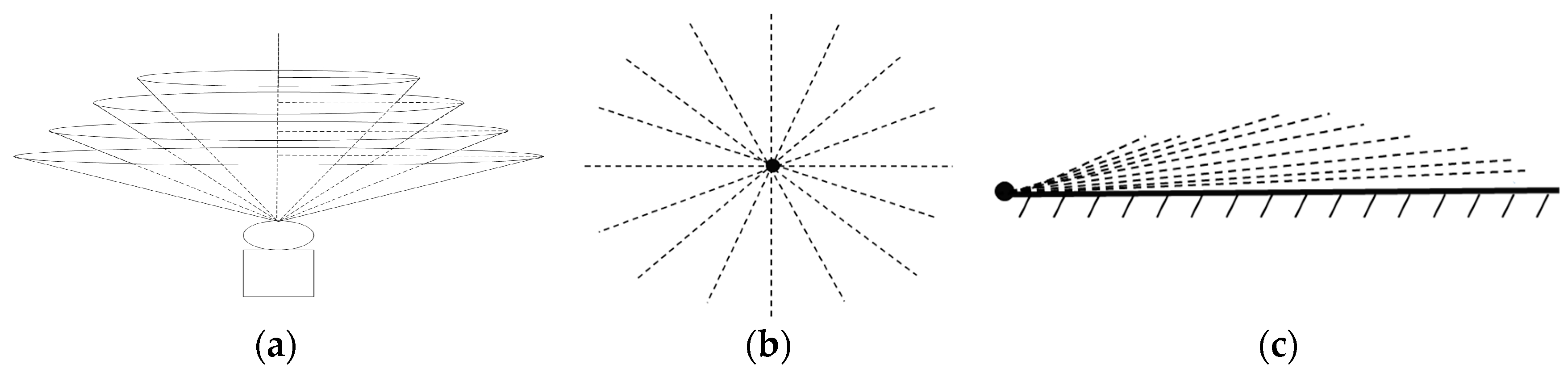
A curved surface space can be regarded as a surface with curved coordinates in space (Figure 2b). The manner of deploying sampling particles in the curved surface space follows similar steps to that of the projection surface space. 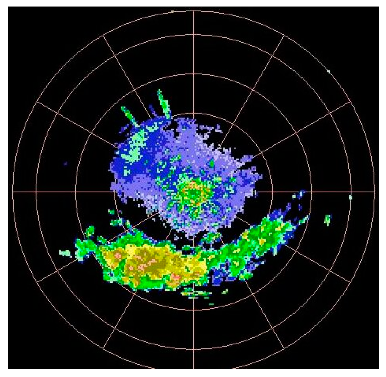For example, for the curved surface space shown in Figure 5, the range of the spatial boundary is determined on the XY projection plane, and the sampling particles can then be set with specific spacing in the direction of the XY coordinate system. As the existing surface is bending, it is difficult to use the expansion mode to form sampling surface cells, as it will cause disconnected fragments. Link mode is more suitable to link sampling particles to fill the whole curved surface space. Accordingly, the meteorological information in each sampling surface cell will be calculated based on the values from its four vertices. This type of spatial lattice model has significant advantages in regard to expressing meteorological information with contour features (such as National Centers for Environmental Prediction (NCEP) re-analysis data).

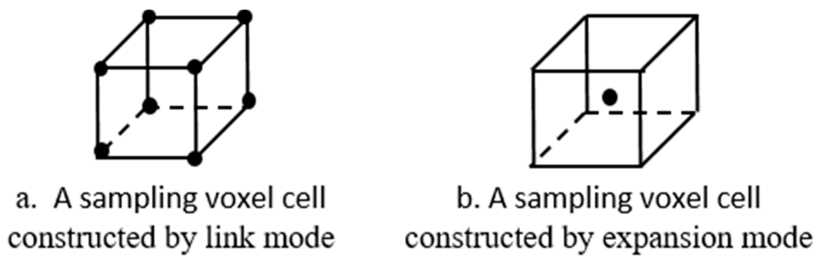
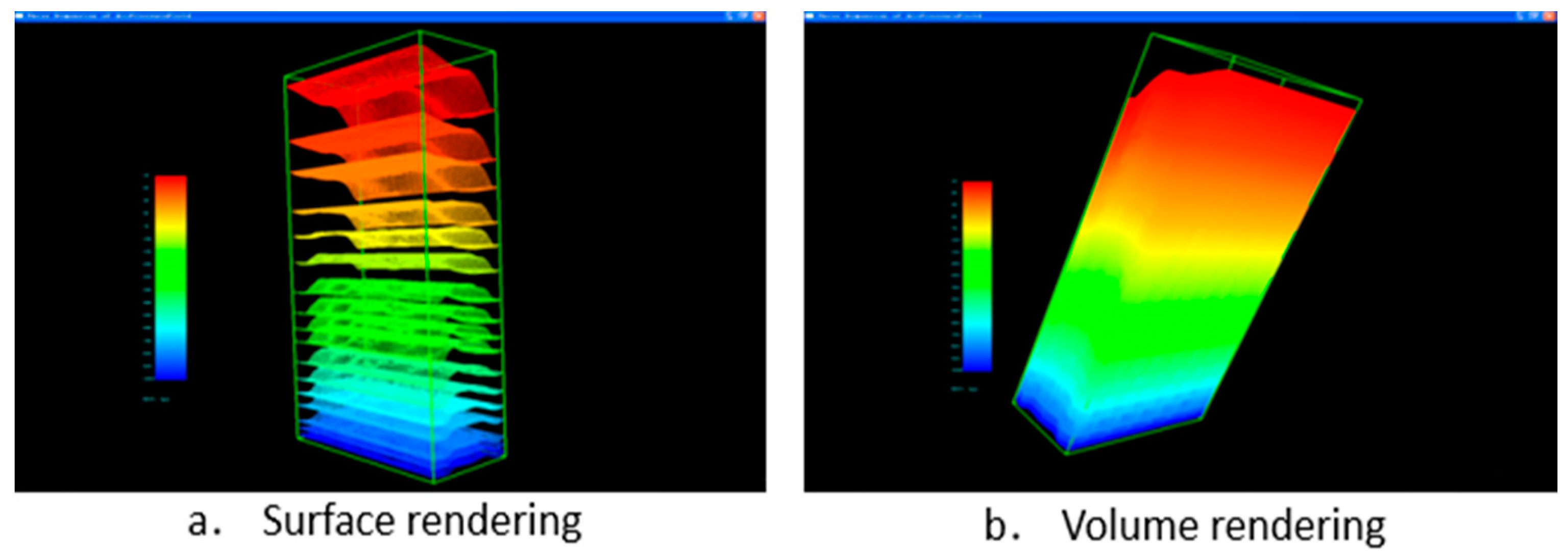
A stereoscopic space is a type of 3D stereo structural space. The corresponding spatial lattice model of the stereo space is a relatively complete one that can compensate for the drawbacks of the 2D projection plane currently used for data expression and analysis in meteorology. It can be constructed by superimposing sampling particles from projection surface spaces (as shown in Figure 6a) or curved surface spaces (as shown in Figure 6b) at different heights. The spatial lattice model constructed based on the projection surface space can be called the projection voxel lattice model, while the one constructed based on curved surface spaces can be titled the curved voxel lattice model. For the former, with its sampling particles, sampling voxel cells can be created by expansion mode (Figure 7a) or link mode (Figure 7b) in three dimensions. However, for the latter, only link mode is suitable for the construction of the curved sampling voxel cells to avoid fragments in the stereoscopic space. The meteorological information of the sampling voxel cell could be acquired by its center sampling particle for expansion mode or calculated by the eight vertexes for link mode. A spatial lattice model for stereoscopic space can be used to describe the characteristics of the 3D spatial distribution of a set of meteorological elements more realistically and provides a concept framework to support the 3D analysis and the processing of the meteorological information.

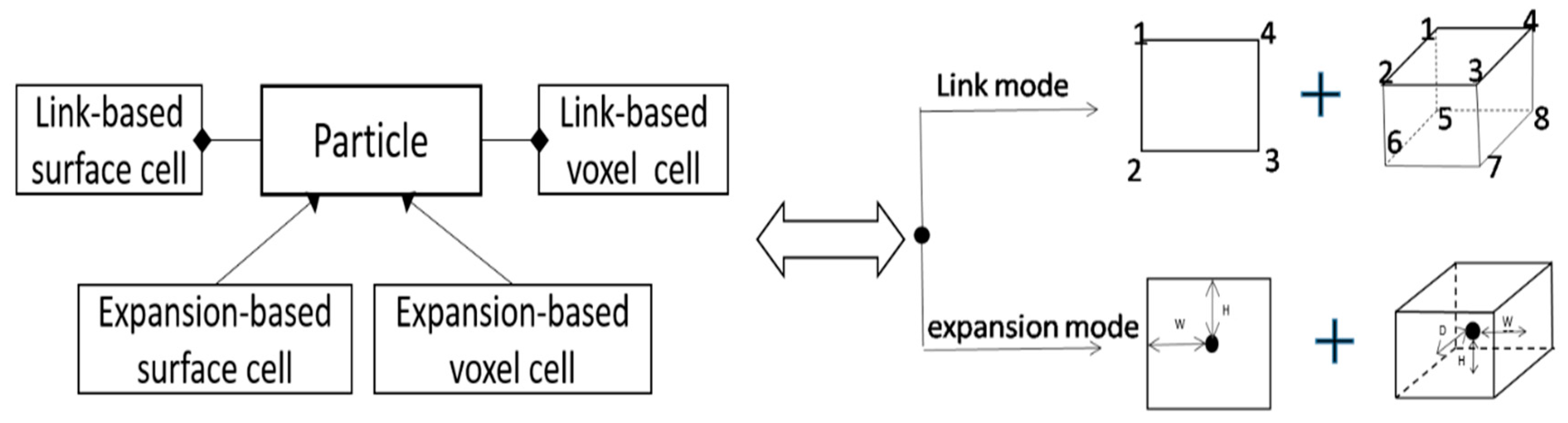
4. Realization of the Spatial Lattice Model

According to the logical analysis above, both sampling surface cells and voxel cells can be constructed using the basic element, i.e., the sampling particle, using either link or expansion mode. To implement the spatial lattice model, the data structure should be designed accordingly (Figure 8).

For those surface cells formed by link mode, the sample particles can be set in a specific order, e.g., anticlockwise order, and the indices can then be recorded in an array to identify different cells. For those voxel cells structured by link mode, the sample particles can be arranged into two layers, and each layer can be regarded as a surface cell. Although this type of storage may cause a problem with redundant data when numerous cells are employed to represent a meteorological space, it is easy to manipulate and will enhance the efficiency of advanced analysis. The exact structure can be designed as

Link-based surface cell: {particles [4], indexes [4] (1, 2, 3, 4)};

Link-based voxel cell: {particles [8], indexes [8] (1, 2, 3, 4, 5, 6, 7, 8)}

where particles [n] is an array to store a set of particles, and indices [n] is used to store the order of particles to construct a cell.

For those cells constructed by expansion mode, because in this work we organize the spatial sampling particles in regular rows and columns, the regular cells can be formed by the center particle and the lengths of its sides. In this case, the exact structure can be represented as

Expansion-based surface cell: {particle, half Height, half Width};

Expansion-based voxel cell: {particle, half Height, half Width, half Depth}

where a particle is located at the center of the cell, and the half Height, half Width and half Depth represent the half-lengths of its sides. Most importantly, different from link-based cells that consist of several particles, this type of expansion-based cell should be designed as inherited from the sampling particle, so it can be regarded as a type of special particle. In this case, it will be easy to expand into a one-dimensional line segment, a two-dimensional surface, and a three-dimensional voxel at a higher resolution when necessary.

5. Case Studies

5.1. Expression of Radar Data and NCEP Pressure Field

Radar data, which are used to describe the reflectivity factor of the raindrops, were employed to verify the proposed model. Using traditional visualization methods (e.g., using principal user processor) [16,17] in the meteorological field, radar data can only be expressed by being projected to a 2D surface plane and saved into a picture (e.g., jpg) (Figure 9). Within the traditional method, the used data model is designed mainly for image mapping. It is difficult to get a “stereo-vision” of radar data, and further analysis is also difficult. At the same time, the classical models are often related to a specific kind of meteorological data processing; there is still a lack of a basic logical model that allows each model to transfer information from one to another.

The projection surface lattice model and projection voxel lattice model were designed to express the surface data. Using the projection surface lattice model, the radar data from a certain scanning sector can be expressed. First, the range and boundary of the research area were determined, and then sampling particles were deployed with a grid spacing of 1 km in the rectangular research area, forming the logical framework for a projection surface with regular row and column spacing (Figure 10a). Then, the meteorological information was attached with different sampling particles by acquiring the original radar data and using double-linear interpolation accordingly to obtain the locations of the particles and radar data grid (Figure 10b). In this case, the whole surface can be attached to meteorological information using a spatial lattice (using point-expansion mode as the FM, and regular rows and columns as the R) and can be expressed (Figure 10c). With similar steps, a projection voxel lattice model was adopted to express the radar volumetric scanning data (Figure 11).

Then, the NCEP pressure field data were employed as another data resource to test the expression capacity of the proposed model. The NCEP pressure data consisted of 17 layers, which are organized in the form of grids. In this study, the curved surface lattice model was first constructed to describe each layer using the row and column spacing, and the 17 constructed layers were then overlapped and expressed by a curved voxel lattice model. The visualization results are shown in Figure 12.

Moreover, normally, the raw radar data detected by the hardware is spatially distributed along rays on the different concentric cone surfaces (about 360 rays in each cone surface) (as Figure 13). To keep the original structure of this kind of data, the practical spatial lattice model should be designed accordingly. In this case, four (for the surface model) or eight (for the stereo model) particles are linked to form a cell to represent the raw radar data. More importantly, the distribution rule R of this practical model can be set as consistent with the original structure of the acquired raw radar data, not in regular rows and columns (as Figure 14a), and thus information in each point of the acquired raw data can be saved following the original structure. The FM is in point-link mode. Figure 14b is the result as a complement to illustrate that the proposed model has the capability to express data with an irregular organization structure.

5.2. Advanced Meteorological Analysis—Taking Cutting as an Case

Since sampling particles are the basic elements of the proposed spatial lattice model, the cutting algorithm can be implemented by grouping different particles, i.e., dividing the sampling particles into two independent groups, based on their attached positions and then constructing independent models for the separate particles in each group for the sub-meteorological space. The most important step here is to find the spatial relationship between the particles and the cutting plane.

Generally, when one point A and a normal vector $\overrightarrow{n}$ in space determine the cutting plane P(A, $\overrightarrow{n}$) for the 3D point object O (shown in Figure 15), the relative relationship of O and the cutting plane P can be determined using Equation (3).

$$F=\overrightarrow{AO}·\overrightarrow{n}$$

(3)

• If F > 0, then, point O is on the positive side of the cutting plane.
• If F = 0, then, point O is in the plane.
• If F < 0, then, point O is on the negative side of the cutting plane.

Since the location of a particle can be regarded as a point in 3D space, a flowchart applying the cutting algorithm for the proposed spatial lattice model of meteorological spaces can be designed as shown in Figure 16.

The spatial lattice model has its specific structure for the organization of sets of particles, and thus, after cutting, the two sets of particles may be stored and they will retain their original organizational structures. Therefore, for the two sets of separate lattice models generated, the expansion mode and link mode can also be applied according to the organization structure for further analysis. From this perspective, each part of the cut particles can be viewed as being generated by removing the particles that are opposite to the cutting plane. Thus, the surfaces generated by the cutting process of the two parts are not smooth but rugged, composed of different cells to form the boundary of the cut volumes. Figure 17 shows the result of performing a cutting operation on the meteorological space created by radar data. Using the cutting operation, the meteorologists can see the inner structures of the storm cloud, which can help them make better forecasting decisions.

6. Conclusions and Discussion

Meteorological space is an important composition of the real world, and the digitalization and analysis of meteorological phenomena are indispensable functions in current advanced tools, such as digital earth [18,19,20] and virtual geographic environments (VGEs) [21,22,23,24,25,26]. In this article, to represent and analyze the multi-dimensional meteorological space, a spatial lattice model was proposed for the visualization and analysis of meteorological information. The meteorological space was then abstracted into the projection surface space, the curved surface space, and the stereoscopic space, and corresponding models were designed. Strategies related to visualization and advanced analysis were illustrated to examine the capacity of this proposed model.

However, there are still some limitations that can be improved in future studies. Firstly, the sampling particles are mainly organized in a common and regular order, but actually, the structure of the meteorological data and the demand for its expression and analysis are actually complex and diverse. Some experiments still need to be conducted to explore setting sampling particles in an irregular order as a supplementary way to test the ability of the proposed model. Secondly, the strategies for data indexing, querying and storage to a database are not taken into consideration in this paper, which would cause data redundancy problems when there is a need to handle a massive amount of meteorological data. For example, a cutting algorithm is performed without the data indexing strategy, but it can be optimized to speed up the grouping process in further studies. Thirdly, more algorithms that can support different types of professional meteorological analysis should be proposed based on this proposed model and used to form an algorithm pool. Lastly, the meteorological space and its elements undergo a continuous evolution with clear spatial-temporal characteristics, but in this article, the parameter t (the time mark) is ignored for simplification. Thus, the capabilities of handling the spatial-temporal meteorological data should also be strengthened in the next step.