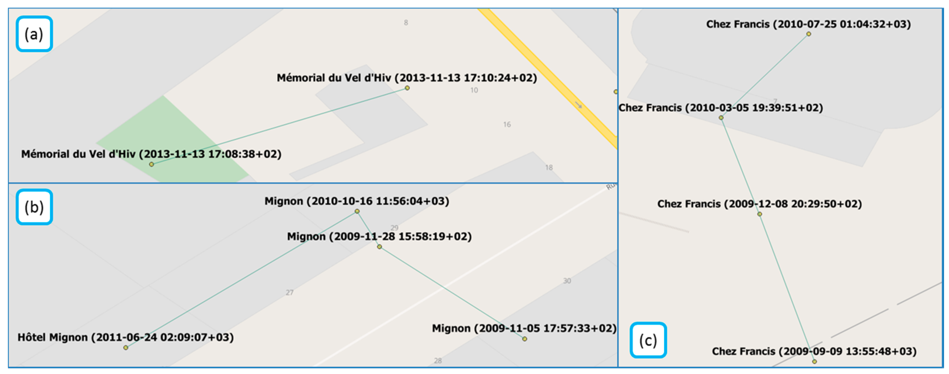
Article

Assessing Crowdsourced POI Quality: Combining Methods Based on Reference Data, History, and Spatial Relations

by
Guillaume Touya
1,*,
Vyron Antoniou
2,*,
Ana-Maria Olteanu-Raimond
1,* and
Marie-Dominique Van Damme
1,*
1
Univ. Paris-Est, LASTIG COGIT, IGN, ENSG, F-94160 Saint-Mande, France
2
Hellenic Military Geographical Service, Evelpidon 4, Athens 11362, Greece
*
Authors to whom correspondence should be addressed.
ISPRS Int. J. Geo-Inf. 2017, 6(3), 80; https://0-doi-org.brum.beds.ac.uk/10.3390/ijgi6030080
Submission received: 5 December 2016 / Revised: 27 February 2017 / Accepted: 8 March 2017 / Published: 14 March 2017
(This article belongs to the Special Issue Volunteered Geographic Information)

Abstract

:
With the development of location-aware devices and the success and high use of Web 2.0 techniques, citizens are able to act as sensors by contributing geographic information. In this context, data quality is an important aspect that should be taken into account when using this source of data for different purposes. The goal of the paper is to analyze the quality of crowdsourced data and to study its evolution over time. We propose two types of approaches: (1) use the intrinsic characteristics of the crowdsourced datasets; or (2) evaluate crowdsourced Points of Interest (POIs) using external datasets (i.e., authoritative reference or other crowdsourced datasets), and two different methods for each approach. The potential of the combination of these approaches is then demonstrated, to overcome the limitations associated with each individual method. In this paper, we focus on POIs and places coming from the very successful crowdsourcing project: OpenStreetMap. The results show that the proposed approaches are complementary in assessing data quality. The positive results obtained for data matching show that the analysis of data quality through automatic data matching is possible but considerable effort and attention are needed for schema matching given the heterogeneity of OSM and the representation of authoritative datasets. For the features studied, it can be noted that change over time is sometimes due to disagreements between contributors, but in most cases the change improves the quality of the data.

1. Introduction

Points of Interest (POIs) describe places of interest for any user of geographic information, such as touristic places, amenities, or shops, and can be easily crowdsourced by citizens. As a consequence, they are often a major part of the contributions of volunteered geographic information (VGI) projects; see for instance OpenStreetMap (OSM) and Wikimapia. However, representing a geographic place that can have an extent as large as a building using the point primitive is not a straightforward process for contributors or even for professional surveyors: what is the best location for a point representing a school that might be composed of multiple buildings? Moreover, crowdsourced data might be subject to frequent, minor or major, changes until a consensus is reached among volunteers. So, only measuring the distance between such POI data and their counterpart in a reference dataset is not particularly meaningful. However, VGI POI datasets do need to be assessed to be effectively used in applications: for instance, when the POIs are to be displayed on a map, the consistency of their location into the vague region they represent is very important to reduce the map reader cognitive load.
From the beginning, assessing data quality was one of the main research topics related to VGI, and particularly OSM (see for example [1]), and is mainly performed through comparisons with authoritative reference datasets [2,3]. Many methods have then been proposed to assess VGI quality; a review can be found in [4,5,6], among others. The quality assessment of VGI POIs is essential as many applications are based on such data, and can be affected by low-quality POIs. POIs from OSM, Wikipedia, or social networks such as Facebook or Swarm can be used for user-centric wayfinding [7], for population analysis [8,9], for land use mapping [10], for urban analysis [11], or for the analysis of people’s perception of places [12].
Despite the aforementioned and ongoing research around VGI quality, there is no holistic and comprehensive framework for assessing the overall quality of such data (research in this direction can be found, for example, in [13,14]) and the existing methods (e.g., ISO-based quality evaluation) are not inclusive or flexible enough to accommodate this new type of data.
The crowdsourced nature of VGI is fundamentally different to classic Geographic Information (GI), not least because there is now a strong social factor behind public contributions and data creation. Thus, it is not uncommon for VGI to suffer from participation biases at all levels of granularity. Moreover, as VGI comes in many flavors and from diverse sources, existing quality evaluation methods do not always provide the means to evaluate them. For, example there are both explicit (e.g., OSM, Geograph, etc.) and implicit (e.g., Flickr, Twitter, etc.) sources of GI [15,16], which, considering the advances in GI retrieval methodologies, can be used to extract meaningful data from all kinds of content available on the Web and thus create innovative spatial products (e.g., from bicycle maps to emotion maps). These spatial products are out of the scope of traditional geo-data producers such as National Mapping Agencies (NMAs) or large corporations.
Additionally, VGI has matured enough to be considered as a replacement of, or as a way to enrich, authoritative data with GI, which has, so far, been missing from authoritative databases. Thus, along with the evaluation against authoritative reference data, VGI needs an autonomous and comprehensive methodology for quality evaluation. In this context, much of the research work has focused on the discovery, documentation, and development of intrinsic VGI quality indicators [4]. In such studies the efforts have focused mainly on a feature-level examination. The examination of the lineage (e.g., versions), of the topology or of the geometric characteristics (e.g., length, area), can result in a basic understanding of overall quality of a VGI dataset.
Following this line of research, this paper examines different ways to evaluate VGI quality. Recent research has proposed methods to evaluate VGI POIs based on history [17] or on comparisons with reference datasets [18], but neither is enough to assess quality alone. In order to assess the potential of combining such methods on POIs, we compare alternative methods on the same dataset. Thus, our first aim is to assess the usability of these methods for VGI POI quality evaluation, and to identify what aspects of data quality each method can or cannot cover. Our second aim is to experiment with a more holistic approach by combining the different methods and identifying what more we can learn regarding quality through this combination. For example, comparing each instance of a feature history against reference data can tell us if new versions of the feature improved its quality.
The remainder of this paper is structured as follows: Section 2 provides an overview of the methodology and the data used. Section 3 evaluates VGI data using their lineage; Section 4 assesses VGI quality using internal spatial relations. Section 5 discusses the quality assessment using data matching techniques by comparing them with authoritative reference data; Section 6 discusses quality evaluation using data from other VGI sources. Then, Section 7 discusses the possibilities when combining the previous methods. Finally, in Section 8, the paper provides conclusions and recommendations for future work.

2. Methodology and Datasets Used

In order to assess the quality of crowdsourced POIs, we used two general approaches: (i) use intrinsic characteristics and measurements derived from the crowdsourced datasets at hand, and (ii) evaluate crowdsourced POIs using an external dataset, that can either be an authoritative reference or another crowdsourced dataset. More specifically, the data under evaluation are the OSM POIs for the Paris region. For the first approach, two methods are proposed for quality evaluation: using the history of each feature alone (Section 3) and analyzing the spatial and topological relationships of the OSM features (Section 4). For the second case, we examined the quality of OSM points against authoritative ones from IGN (The French Mapping Agency) by using a data matching algorithm (see Section 5) and by using geo-tagged photographs from Flickr (see Section 6). Finally, all these evaluation methods were combined to improve the analysis of data quality and generate new knowledge (see Section 7).

2.1. OpenStreetMap Dataset

The OSM project is one of the prime examples of crowdsourcing GI. Since 2004, the OSM project has mobilized contributors from around the globe in order to create a freely available geographic database. Today, there are more than three million registered contributors in OSM and despite the fact that the vast majority are occasional contributors and thus only a small fraction of them is consistently contributing, on a monthly basis, there are more than 20,000 active contributors (at the time of writing); this constitutes a huge workforce. The initial aim was to enable volunteers to use their local knowledge to capture geographic data for areas they know. This has since expanded and volunteers are now mapping areas worldwide due to technological advances and the open availability of very high resolution satellite and aerial imagery. This development has boosted the expansion of OSM with the tradeoff that the influence of local knowledge is diminishing in OSM data. Nevertheless, OSM is still the most up-to-date crowdsourced global geographic database today and the data are used in diverse applications from aiding humanitarian efforts [19] to use in governmental projects [20].
The OSM data model consists of three vector-based geometric primitives. The first are nodes, which are point-based and are used to capture either individual points (e.g., landmarks) or are part of the second primitive, i.e., a way, which is used to capture either linear or polygon entities. Finally, relations are used to the capture logical collection of nodes, ways, or other relations. For each of these primitives, the OSM data model allows attributes (commonly referred to as tags) to be attached using a key:value form. While a fundamental OSM principle is that contributors are free to choose whatever attributes they want, in practice there is a wiki-based specification for the OSM project that provides suggestions and best practices about the combinations that should be used in each case. Another important element of the OSM data model is that the geographic database itself is created in a wiki-based manner. This means that all contributors can edit all existing features and that all the previous versions of a feature are available, along with details for each version (e.g., when it was created, by which user, which tags were assigned to the feature, etc.). OSM provides an Application Programming Interface (API) that enables access to the geographic data, data about the contributors, and data about the individual features and their previous versions.
For this study, OSM data were downloaded for a case study area in the Paris region. The coverage of the selected area is quite complete due to the presence of an active OSM community. To download the OSM data, the Geofabrik shapefile download service was used. Although there are some differences between the OSM and Geofabrik repositories (mainly due to the exclusion of non-standard tags), these differences will have no effect on our methodology. As the scope of this paper is quality evaluation of point-encoded features, and in particular the geometry, the name and the types of the OSM points, only the layers of Places (4275 features) and POIs (192,228 features) were assessed. The Geofabrik shapefiles include, as an attribute, the original and unique OSM_ID of every OSM feature; this information was used in combination with the OSM API. For example, the entire history of the OSM feature with OSM_ID 26691437, can be accessed using the API request: http://api.openstreetmap.org/api/0.6/node/26691437/history/. The API response is an XML file that includes all the versions of the feature with OSM_ID 26691437. Through an iterative process, all the versions of each OSM features in scope were downloaded and stored in a PostgreSQL/PostGIS database. This method provided a complete timeline of the OSM edits made in the area for the data of interest.

2.2. Reference Dataset

The reference data were extracted from the BD TOPO database produced by IGN. BD TOPO is a topographic dataset with a positional accuracy below 1 m. Its scope does not cover all POIs that are captured in OSM (e.g., there are no shops or restaurants), but the POI layer covers education, administration, transportation, religion, health, sports, and hydrography, which gives a sufficient overlap with OSM POIs for comparison purposes. The attribute values, originally in French, have been translated to English to enable semantic matching with OSM. The IGN POI dataset contains 6202 features. The change in IGN features is due to updates (e.g., a change in the real world, errors correction), changes in specifications or changes due to partnerships that provide data to IGN (e.g., Ministry of Education for the position of schools, RAPT for the local public transportation administration).

2.3. Flickr Dataset

The development of Web 2.0 [21] has led to a bi-directional Web where the aim of many web-based applications is to provide platforms that enable users to create and publish their own content and share this with other users. This development has led to the emergence of social networking websites. One of the first examples of such websites have been photograph sharing applications, e.g., Flickr, Picasa Web, or the more recent Instagram, which urges users to share their photographs along with titles, comments, keywords (known as tags), and their location (known as geo-tagging), and then to use them as means of networking. While geography or the location of the content is not the prime feature of such applications, they can still be implicit sources of GI since newly developed GI retrieval methods can transform implicit information into geospatial content [22]. In this study, geo-tagged photographs downloaded from Flickr have been used to evaluate the validity and quality of ambiguous OSM features. By using the Flickr API, all geo-tagged photographs uploaded to the Flickr website between April and December 2015 have been downloaded, resulting in a total of 79,722 geo-tagged photographs to help determine the presence and type of OSM POIs that cannot be identified using satellite imagery (e.g., POIs located under trees or the type of buildings).

3. Assessment by Historical Analysis

Research into geometric intrinsic evaluation indicators has focused on different aspects of position and topology (see also Section 4). For example, van Exel et al. [23] examined the provenance of OSM features as an indicator of their quality. Feature length and point density have been used by Ciepłuch et al. [24] to analyze OSM data quality. Keßler and de Groot [25] examined feature-level attributes that are specific to VGI (and not applicable to authoritative data) such as the number of versions, the stability against changes from other contributors, and the number of corrections or rollbacks of OSM features. Barron et al. [14] presented a framework that provides multiple intrinsic indicators, based solely on the data history of OSM, which helps in the quality assessment.
Here, we examine the type, name and geometric lineage of OSM point-encoded features (i.e., Places and POIs) for the study area. Thus, the possible changes in an OSM point that are of interest for this study, are those that could affect: (i) its type, for example, a feature initially characterized as a town can later be changed into a city or village; (ii) its name, where a feature’s name can undergo either a major or a minor grammatical change (e.g., the place name ‘St. Louis’ could change to ‘Saint Louis’ or to something totally different); and (iii) its location, where a feature can be moved by the contributors by just a few centimeters up to hundreds of meters away. Thus, the possible states of an OSM point are either to be stable through its entire life-cycle or to have a change in one or more of the three abovementioned factors. For the present POI assessment by history analysis, we selected only named places and POIs (4273 and 53,052 features, respectively).

3.1. Methodology and Results

To evaluate the quality of OSM points (that have a name) over time, we used the history (i.e., OSM versions) of each feature so as to examine the types and level of change. The ability to replicate the state of an element at any particular point in time enables both qualitative and quantitative assessment of the type and magnitude of the changes.
First, we counted the features affected by different types or combinations of changes for OSM Places and OSM POIs. Then, we examined the magnitude of change for selected cases. For the OSM Places we calculated the following: (i) the percentage of displaced features per feature type (e.g., what percentage of towns have a positional change over the years); and (ii) the overall displacement (in meters) per feature type. For OSM POIs we calculated: (i) the percentage of displaced features per feature type; (ii) the percentage of name changes and location changes per feature type; and (iii) the displacement (in meters) of features per feature type.
The magnitude of displacement of a feature is defined by the distance between the centroid derived from all known positions of the place (for its entire life) and its last position. Figure 1 shows examples of the positional change of POIs along with the entity names and the creation date of each point version.
By following this methodology, we tried to determine how named OSM POIs behave during their life time. While this is not an exhaustive analysis, it nevertheless lays the groundwork for an understanding of how different feature types behave and thus what assumptions can be made regarding their quality over time.

3.2. Assessment of OSM Places

Places and toponyms are a valuable element in many different products including gazetteers, in cartography and for mobile applications, location-based services, and search engines. Thus, any kind of change in the data will affect the consistency of products or services that use VGI.
The analysis regarding the different types or combinations of possible changes showed that two-thirds of the features (66.8%) remained unchanged. The most common change is recorded in the geographic position (12.3%) of the features, followed by a combined change in the position and name (7.8%). Interestingly, the analysis of the percentage of displaced features per type showed that different types of OSM places have different behaviors. A case in point is the OSM feature town where 80% (i.e., 198 out of 248) have been geographically moved over time while only 8% of the feature locality has undergone a change in their position. The analysis of the magnitude of the positional displacement per feature type showed that features with large spatial extent face large changes in their location in contrast with smaller entities. For example, 21% of the features having the type suburbs moved less than 100 m, whereas for only 2% of the suburbs a positional change of more than 1000 m was recorded. In contrast, 14% of all features in the towns category have moved more than 1000 m.

3.3. Assessment of OSM POIs

Only lately have POIs found their way into spatial applications. Traditional map-making processes excluded this type of information, not because of importance but rather because maps, and especially paper maps, were built as long-lasting generic products aiming to support multiple applications due to the high cost and extensive knowledge needed to construct them [26]. However, the advent of VGI has enabled citizens to easily capture and put local information on a map. Much of this information comes in the form of POIs. Usually, apart from the location of the POI, contributors can add various attributes such as its name (if applicable) or its type (e.g., bank, hospital, coffee shop, etc.). From the POIs extracted from OSM for the study area, (i.e., 200,000), only 27.6% of them (i.e., 53,052) had a name attribute. This is an expected result since POIs are part of a heterogeneous spatial layer that can include world-known landmarks and monuments as well as local street junctions and traffic lights where a name attribute is not applicable.
As described in the methodology, the changes in location, type, name and any possible combinations have also been examined for POIs. The analysis shows that about 60% of features have not been changed since their creation, while the most common change for POIs is a change in the name (13.2%), followed by a change in the location (12.7%) or in both location and name (10.2%). The rest of the changes correspond to less than 2.0% each.
Given that the two most frequent feature changes are the changes in name and in location, and examining this from the point of view of individual categories (i.e., OSM types), it is interesting to see which POI categories are changing more and how much they are changing. Figure 2 shows the percentage of OSM POIs that have undergone a name and a location change grouped by POI category for the 20 most popular categories. This visualization of the volatility of each category can be linked to the fitness for purpose of various categories beyond the strict, tangible measurements of quality elements (as defined in [27]). For example, the station category is an extremely volatile category as 59% of the features have changed position and 76% have changed name. The analysis described in Section 5 will show that this category is a complex one, and can help to explain the high volatility in the feature of this category. The number of changes also reflects the popularity of the features since stations are used by most users from this area. Any application or products aiming to incorporate these features should take into account these possible changes. In contrast, POIs related to information prove to be much more resilient to change.
Table 1 and Table 2 show statistics of the positional movement of the ten OSM categories ranked by the highest movement. The aim is once again to understand the fitness for purpose of different categories for different applications. For example, for the station OSM features that have experienced a change in their location, the average movement is almost 40 m whereas for bakery it is a mere 4.7 m. However, in all cases the standard deviation is bigger than the (arbitrary) threshold of the 10 m accuracy that hand-held GPS devices can achieve. In parallel, the maximum positional movement recorded shows that, in some cases (e.g., supermarket or stations), the contributors might disagree on where the best place is to position the point that will represent the physical features since the area of the feature might be quite large (see the next sections for more discussion of this point). For other cases such as café, bakery, hotel, and bank, which are characterized by small and precise geographic extents, the maximum distance shows that there have been some gross errors made by contributors that have been corrected in a later version (or vice versa). However, the notion of gross error is somehow elusive and certainly not uniform in these datasets. For example, a maximum displacement of 339 m for a point that represents a hotel might be a valid movement since both points could be inside the spatial footprint of the hotel. Even in the case where one of the two positions is a wrong measurement, again a visual inspection would be needed to determine whether the magnitude of the displacement falls under the “gross error displacement” or whether it is an acceptable error. Thus, it was decided to include all the positions in the calculation of the descriptive statistics presented in Table 1 and Table 2, which will also allow the reader to understand the magnitude of the volatility of such data.

4. Assessment by Analysis of Spatial Relations

4.1. Methodology

Another way to carry out intrinsic quality assessments of VGI is to rely on the geographic properties of features [28]. If we find expected spatial relationships within the VGI features, e.g., a motorway junction is at the intersection of a motorway and another road, the quality tends to be good. On the contrary, if we find impossible or improbable spatial relations within the features, e.g., a shop POI is outside a building, then the quality tends to be poor. This use of spatial relations to guide the quality assessment has already been implemented in [29]. However, the main problem is that POIs are points that represent a geographic entity that has a geographic extent often much larger than the point, so, for example, where do we put a point that represents a school: in the school boundaries, at the entrance of the school, or in the middle of the school? There is no unique solution to this problem (Figure 3), and we propose different methods for different types of POIs in the next sub-sections. This will improve overall quality as it will improve the consistency of the contributions.

4.2. Amenity POIs

There are many types of OSM amenities but not all are facilities located inside a building. We did not consider amenities that can be located outside a building, such as food trucks. Thus, we consider that their quality is good if they are inside a building, and if they are located on the part of the building occupied by the amenity. There are two ways to capture such amenities: put the POI at the center of the amenity, or at the entrance of the amenity. Thus, we propose to check three spatial relations (Figure 4):
  • inside a building;
  • distance to the building center;
  • distance to the nearest building boundary, as a proxy for amenity entrance.
Figure 5a shows that the building center is not always a good approximation of the amenity center, as several amenities can share a building. Thus, we also computed the Voronoï regions around the amenity points (Figure 5b) and intersected the buildings with the Voronoï regions (Figure 5c). Then, we also computed the distance to the center and to the boundary for these new regions. We selected four types of amenities (around 6500 POIs in the Paris dataset):
  • very small amenities: gift shops, i.e., the features tagged with “amenity = gifts”;
  • medium amenities: bars (“amenity = bar”), cafes (“amenity = café”), and restaurants (“amenity = restaurant”);
  • large amenities: cinemas (“amenity = cinema”);
  • very stable amenities: hairdressers (“amenity = hairdressers”) that do not move often, according to [17].
The results, summarized in Table 3, show that precision is somehow related to the size of the amenity, which is logical as there is more room to locate a POI inside large amenities. It can be noticed that the percentage of amenities that are outside buildings ranges from 1.5% to 5%, and thus these POIs have a low positional accuracy (gift shops are too few to be significant here). The numbers are quite similar in all the small/medium amenities, i.e., they are quite far from the center, even with Voronoï regions, with a large variability, and there appears to be a pattern with POIs located close to the boundary/entrance, but just inside the buildings (around two meters). This can be explained by the way that the amenity symbol is visualized in the OSM map as the symbol appears just at the entrance of the building with this 2-m shift.
It would be logical if the POIs inside the same buildings were consistent with each other, i.e., located similarly at the center of the amenity, or at the entrance (Figure 6), because either the contributor is the same or the first contributors direct the following contributors. Thus, we checked this assumption for more than 4000 buildings in Paris that contain more than two POIs.
The results, summarized in Table 4, show good homogeneity inside a building. There is some standardization: POIs are located closer to boundaries than to the center but not on the boundary. However, even with an accurate standardized location, the precision is quite low, as shown in Figure 4.

4.3. ATM POIs

In the city of Paris, most ATMs are located on the walls of banks and only a minority are located inside a bank building. Thus, a logical positioning of the ATM POIs would be just on the boundary of the building polygons. We used the same methodology as that used for amenities to compute the building center, and we measured the distance to the center and to the boundary (Table 5). There were 347 ATMs in the dataset and 6.6% of points are outside any building: these points clearly are poor quality because the building layer has good completeness, which was confirmed by a visual inspection of those points. Sixty-five percent of the ATMs lie just on the boundary of buildings, so there is a vast majority of points with a good quality. There are an additional 6% that are both far from the center and from the boundary, so they are considered randomly and badly located. We also carried out the same test for consistency in buildings that contain several ATMs; the results show that ATMs are mostly consistently located inside a building but when one is located on the boundary, all are located there, with very few exceptions.

4.4. School POIs

Schools are complex functional entities composed of buildings, schoolyards, sports fields, libraries, and even chapels [30]. Ideally, we need to know the complete extent of the school and its components to assess the quality of the school POI position: in Figure 7, the POI is located in the schoolyard, so not inside any building, but it is close to the school extent centroid. Unfortunately, extent polygons are not available for all school POIs in this dataset: only 23% of the 438 schools are captured with both a POI and a polygon. The difficulty of assessing school POI quality due to the complex structures of schools is highlighted in [31], the authors of which tried to match several school POI datasets from different VGI or reference datasets.
When a polygon extent was available for the POI, we measured the distance to the center of this polygon and to its boundary; when none was available, we used the building that contained the POI, as we did for amenities and ATMs. The results, summarized in Table 6, show that, when the polygon is available, the POI is closer to the school center and so more likely outside buildings; when the polygon is not available, OSM contributors tend to map the school POIs closer to the walls, at the entrance of the school. However, with 30% of POIs outside a building, it would be better to use the real school extent, which can be computed geometrically by aggregating the nearby buildings and geographic entities, using their likelihood of belonging to the school (e.g., a building that contains shop POIs is unlikely to be part of the school). The same approach was successfully used in [32] to adjust the geometry of such school extents for cartography. When a polygon is available, the contributors tend to locate the POI closer to the center, but the size of the school implies low precision.

4.5. Bus Stop POIs

In Paris, bus stops can be marked either by a bus shelter, as in Figure 8, or by a sign, but they are always located on the pavement, so there is a minimum distance between the bus stop and the closest building boundary and between the bus stop and the road centerline. There is not enough information in the OSM data to check if the bus stop is on the pavement, but we can check that it is not too close to the nearest building boundary or the road centerline. We also want to measure whether there is a road close to the bus stop, because there is no bus stop without a road nearby.
We used 1.5 m as a minimum distance between the bus stop point and the nearest building boundary. The minimum distance to the road centerline depends on the road type but a 2-m threshold is used here. In parallel, as large roads are captured with several lanes in Parisian OSM data, we used 10 m as a threshold for being too far from any road. Table 7 shows the results obtained on the 2022 bus stop points in the dataset. Of these, 13.5% of the bus stops are either too close to a road or a building (since they cannot be both), and are considered to be badly located. Only 0.4% are too far from any road. The results show consistent locations in the remaining bus stop points, which can be explained by the fact that bus stops are entities with a small geographic extent, and are easy to spot from high-resolution satellite imagery.

5. Assessment based on Data Matching with Reference Data

A number of research papers dealing with VGI data quality assessment have compared crowdsourced data with reference data to infer their quality [2,3,33]. The comparison of two datasets supposes that homologous features (i.e., features representing the same object in the real world) are first identified. This process is referred to as data matching. In this paper, we propose using a data matching algorithm defined by [34] to automatically detect homologous features between OSM and IGN POIs. The method, which uses belief theory, combines different criteria based on geometry, thematic and semantic properties.

5.1. Methodology

To compare IGN and OSM POIs, we first identify the types of features that are represented in both datasets. As shown in Figure 2, stations and subway entrances are types of objects that have relevant changes regarding names or positions and they are represented in both datasets. Thus, we focus the data matching on stations representing subway stations and subway entrances.
Figure 9 illustrates the data model for subway station representation and defines the links between the real world and the two representations from IGN and OSM. Thus, a subway station in the real world (represented in the blue box) is characterized by a name and a certain number of subway entrances and exits. Regarding the representation of subway stations in the two datasets, two main differences can be noticed. In the IGN dataset (green box), a subway station from the real world is represented by n features. Thus, with respect to the IGN data specification, two types of mapping for each subway station are possible: (i) for subway stations without a connection between several lines, only one point feature is represented in the dataset; (ii) for subway stations that connect to at least two subway lines, at least two feature points are represented in the dataset. Even if the concept of entrance/exit does not exist in the IGN dataset, the features representing the subway station are frequently located close to an entrance.
On the other hand, in OSM (purple box), a subway station in the real world is represented by m features belonging to the OSM type station. The subway station is composed of m’ entrances/exists represented by a point feature, each entrance/exit having a name. In Figure 9, dotted lines illustrate matching links (i.e., features representing the same object in the real world and numbers illustrate the cardinality of the matching links (e.g., n IGN subway stations should be matched with m OSM subway stations). Given the complexity of the representation of the two datasets, many types of data matching links are possible but we are interested in two types of data matching links in this study. First, n:m links are defined for the concept of a subway station (i.e., n IGN subway points can be matched with m OSM subway points representing the same subway station). Second, m:m’ links are defined for a subway station and its entrances/exits (m OSM subway stations are matched with m’ OSM entrances/exits). Finally, 1:1 links are defined for entrances/exits (1 IGN subway station is matched to 1 OSM entrance/exist).
Figure 10 shows an example of two different representations in the IGN and OSM datasets. For example, Duroc subway station (Figure 10a) has one point in OSM data and two points in the IGN dataset that are closer to two subway entrances in OSM (‘Duroc—sortie 3 place Léon-Paul Fargue and ‘Duroc—sortie 1 boulevard des Invalides’). On the contrary, for Saint-Sulpice subway station, one point is mapped in both IGN and OSM data but there is no link between the IGN subway station and the OSM subway entrance. In Figure 10b two OSM entrances can be seen near the OSM subway station; one of them can be considered a duplicate entrance and should be removed.
The data matching algorithm works as follows: for each reference feature from a dataset, the algorithm looks for candidates (from the comparison dataset) to match using a buffer. Then different similarity factors are compared between the reference feature and all selected candidates. Knowing the characteristics of our datasets (see Section 2.1 and Section 2.2), three criteria were used: position, toponym, and semantic criteria. The position criterion is based on the distance between the reference feature and a candidate. The toponym criterion compares the name of the reference feature with the name of the candidate. Among the different measures tested to compare names, the normalized Levenshtein distance was used since it was considered the most suitable for our dataset. Finally, the semantic criterion, which compares feature types, was used to select features in both datasets that represent the same type of objects in the real world, in our case: subway stations, stations, and subway entrances.
The data matching described above was applied on different datasets: (i) subway stations from IGN with OSM stations (link * in Figure 7, n:m cardinality) and (ii) public stations from OSM with subway entrances from OSM (link ** in Figure 7, m:m’ cardinality). In the first case, the reference feature is IGN and the candidate features are from OSM, while for the second case the reference feature is OSM subway entrances and the candidate features are OSM stations.
The thresholds used in the matching algorithm were defined with respect to data characteristics obtained by analyzing the distributions of the distances for each criterion. Thus, the threshold for the position criterion (Euclidian distance) and the name similarity criterion (Levenshtein distance), which indicates that it is unlikely for two features to represent the same object in the real world, are equal to 220 m and 0.6, respectively. The buffer for the candidate selection was set to 350 m.

5.2. Data Matching Results

The data matching results and their evaluations (manually checked) are provided in Table 8. Thus, the results for the first matching (i.e., IGN subway stations and OSM stations) are quite good. Out of 329 IGN subway stations, 328 were correctly matched with their homologous features in OSM stations.
Figure 11 illustrates a data matching result for both IGN and OSM stations (blue link) and OSM stations and entrances (yellow link between a subway station and its entrances). The subway station Châtelet is represented by two features in IGN data and one feature in OSM data. The link between homologous subway stations having a cardinality of 2:1 is illustrated in blue. Twelve OSM entrances are matched with the OSM subway station ‘Châtelet’. The link, with a cardinality of 1:12, is represented by yellow lines in Figure 11. We can see that the homologous subway stations are quite far away from one another, i.e., 140 m and 180 m from the IGN subway station.
Among the non-matched IGN subway stations, seven of them are correct (i.e., there is no homologous subway station in OSM) and two of them are wrong (i.e., they should be matched to a station from OSM). The features are not matched because the distance between homologous features is high and the names are quite different; see Figure 12a to see one of the non-matched IGN subway stations.
For 10 of the IGN subway stations, no decision has been taken. This is due to the fact that for an IGN subway station there are many OSM candidates with the same characteristics. For example, in Figure 12b the IGN subway station ‘Concorde’ has three candidates in OSM that have the same name and are close to IGN subway station. This is definitely a limitation of the data used and the matching algorithm for each of the n:m cardinality links.
Of the total OSM stations, 408 were not matched. This is generally due to the fact that the OSM station category includes not only subway stations but also other types of public transportation in the Paris area such as trains, RER, etc.
The second line of Table 8 summarizes the results for data matching between OSM subway entrances and OSM subway stations. Of 794 OSM subway entrances, 701 correspond to at least one OSM station. All these links have been manually checked and validated (precision = 100%). The recall index is not computed for this case because there is no ground truth regarding the number of entrances and exits for each subway station. Regarding the non-matched results, 19 OSM subway entrances are not matched by the data matching algorithm but all of them have at least one corresponding OSM station. In this case the data matching algorithm fails because the subway entrances are far from the corresponding station and most of the non-matched OSM subway entrances do not have a name (attribute omission).
Similarly to the data matching between the OSM and IGN subway stations, the 74 subway entrances are not matched because no decision was taken. This is due to the fact that for an OSM subway entrance many OSM stations candidates exist that have the same characteristics.
The two matching results define the homologous features between IGN and OSM subway stations and define links that assign entrances and exits to each OSM subway station. Thanks to these two results, it is possible to define the link between IGN subway stations and OSM subway entrances/exits. These three links will be used to assess the quality of subway stations and subway entrances from OSM.

5.3. Positional Quality Assessment Based on Data Matching Results

To assess the positional quality, the Euclidian distances between homologous objects in IGN and OSM data are first computed. Figure 13a shows that the homologous subway stations are quite far away from one another. The median distance is equal to 35 m (50% of homologous features are located less than 35 m away) and for many OSM subway stations the distance is higher than 100 m. Second, the distance between each IGN subway station and its nearest OSM subway entrance is computed. Figure 13b clearly shows that IGN subway stations are closer to OSM subway entrances than OSM subway stations. This fits to IGN specifications (i.e., a subway station location represent an entrance) and illustrates the complexity of these types of features. When the IGN subway station is closer to a subway entrance, then distances are around 80 m. Finally, when an IGN subway station is closer to an OSM subway station, then the distances are equally distributed across a 50-m interval.
In addition, the data matching and the evaluation of results allowed us to identify the following omissions:
  • one OSM subway station (‘Pont de Neuilly’) is not mapped. It is important to note that this station was added during 2016, after we had extracted our OSM dataset .
  • 13 OSM subway stations do not yet have subway entrances.
  • two OSM subway stations have duplicate locations (exactly the same position).

5.4. Thematic Quality Assessment Based on Data Matching Results

In contrast to the positional quality, the thematic quality seems to be better as revealed by the comparison between names of homologous subway stations. To compare the names, the Levenshtein distance was used. The distance is zero when the names are exactly the same and equals 1 when they are completely different. As can be seen in Figure 14, almost all homologous subway stations have the same name (median of Levenshtein distance is zero). Of the 329 matching links, 257 have a Levenshtein distance equal to zero. When this is not the case, the following situations can be observed:
  • For 17 subway stations, the IGN name is too detailed, such as ‘Goncourt (Hôpital Saint-Louis)’ (IGN) versus ‘Goncourt’ (OSM), ‘Pont Neuf (la Monnaie)’ (IGN) versus ‘Pont Neuf’.
  • The type of station is integrated in the name for OSM subway stations such as: ‘Charles de Gaulle Étoile (RER)’, ‘Gare de Lyon (métro 1)’.
  • Different nomenclature is used: ‘Palais Royal (Musée du Louvre)’ for IGN versus ‘Palais Royal – Musée du Louvre’ for OSM.
We have noticed that the naming convention of OSM subway entrances more or less follows a standard: Name of the subway station—Exit nn—street xxx. Thus, we were interested to see how closely this standard is followed. The following cases are observed:
  • case 1: OSM subway entrances that contain the name of the OSM subway station.
  • case 2: OSM subway entrances have the same name with the corresponding OSM subway station where the latter has at least two subway entrances. This case can help identify OSM subway entrances for which the name should be distinguished from the name of the OSM subway station (because the subway station has more than two subway entrances) but is not.
  • case 3: OSM subway entrances for which the name contains ‘exit xx’ or ‘−xx’.
The results for these three cases are given in Table 9.
In addition to the previous analyses, the data matching and the evaluation of the results allowed us to identify the following omissions:
  • for one OSM subway station the name has not been filled in;
  • 121 OSM subways entrances have no names.

6. Assessment by Checking Complementary VGI Sources

As discussed in the previous section, a common approach to assessing the quality of VGI data is comparing it against authoritative datasets. This method enables the use of existing quality evaluation methods and has a number of advantages that can provide a comprehensive understanding of VGI, it can reveal any patterns or biases that might exist in the data (e.g., number of contributions and level of participation in rural vs. urban areas) or it can document, in a tangible way, the agreement of VGI data with authoritative, and thus asserted and trusted, spatial data.
However, there are some equally important disadvantages. First, authoritative data are not always freely available or come with restrictive licensing agreements. Secondly, in some cases, VGI datasets are more current than the authoritative ones and thus omission and commission errors are hard to assess. This problem is intensified by the fact that VGI can be more detailed regarding certain features (e.g., bicycle rental points) or in certain geographic areas (e.g., popular or touristic areas). Moreover, in many cases, the lack of specifications in VGI products leads to heterogeneous data that prohibit straightforward comparison with authoritative data. Finally, VGI projects, such as OSM, can be more accurate and more complete than authoritative data (especially in developing countries), which violates the basic assumption of using authoritative data as reference data [35].
All these reasons gradually transfer the onus of VGI quality assessment to the contributors. Although this concept is a core part of VGI projects, participation and contribution biases do not allow for a uniform quality assessment (see for example [1]). Moreover, even when contributors want to help in quality assessment, there are cases where this is not always possible, especially when this is done remotely through the use of satellite imagery for features and attributes that cannot be shown in the images (e.g., attributes, names, hidden or not visible features, etc.) and thus cannot be extracted by photo-interpretation. Finally, there are cases where, for the same or adjacent features, there are contributions that are contradictory or not topologically feasible. Again, in such cases the pool of contributors and contributions from a single VGI project might not be enough for the quality assessment of VGI.

6.1. Methodology

In order to cover this gap in quality assessment, we used data from other sources of implicit VGI content to evaluate the validity and quality of OSM POIs. For this role we chose the geo-tagged photographs available from Flickr. The combined view of OSM POIs and geo-tagged photographs can help to evaluate the quality of the OSM POIs and disambiguate inconsistencies or contradictory contributions, especially when the time-stamp available in both VGI datasets are taken into consideration. This evaluation was made manually for OSM POIs that are not directly visible from satellite imagery (e.g., POIs that are under wooded areas).

6.2. Results

We used the IGN dataset for the wooded areas of Paris in order to spot the OSM POIs that are not visible using satellite imagery. Those POIs cannot be evaluated or corrected by contributors unless they physically visit the location. However, taking into consideration the Pareto principle, which also applies to VGI contributions [36] and dictates that a small percentage of volunteers generate the vast majority of content, as well as the participation and spatial biases of the contributors, it is understandable that quality evaluation or update of “hidden” elements is a challenging issue. In this context, we manually examined whether the use of geo-tagged photographs can provide additional information for POIs that are not directly visible from remote sensing. Figure 15a shows the OSM map for an area in Paris (‘Musée Rodin Gardens’) where a number of POIs are under trees. Figure 15b shows the same area with the IGN polygons of the wooded areas and the position of geo-tagged Flickr photographs. The Flickr photograph is shown as a pop-up with additional attributes provided by the photographer.
The above example show that the combination of different sources of VGI data can offer a better understanding of the underlying reality, allowing the evaluation or update of volunteered content. However, manual evaluation is cumbersome, and thus, as a second step, we developed an ad hoc application that uses distance between points to detect the possible combinations of geo-tagged photographs and hidden OSM POIs and then asks the user to respond whether a particular POI (according to OSM) can be recognized in a photograph that is taken from a close distance (e.g., ‘Do you see a bus-stop about 4 m away, in the photo below?’) where the attribute ‘bus-stop’ comes from the OSM POI and the distance of 4 m is the distance between the OSM POI and the geo-tagged photograph. We manually evaluated 1000 pairs (i.e., POI—geo-tagged photograph) and it was possible to positively recognize and evaluate 78 POIs. In these cases, the POIs could be positively identified and thus evaluated for their existence and validity.

7. Combining the Methods

All the presented methods give an insight into the assessment of the quality of VGI POIs from a different point of view, but none is really able to provide a generic framework. Reference-based methods require reference data, which are not always accessible or might not exist at all. History-based methods, cannot distinguish between high quality features made from the first edit and features that require further edits to improve quality. The combination of different VGI sources can disambiguate or verify problematic cases up to a certain level, while spatial relation-based methods are good at finding outliers such as amenities outside buildings but are dependent on existing data to provide a finer-grained quality assessment (e.g., school POIs would be better assessed if school polygons were available). Some other POIs are hard to assess because there is no generic spatial relation that can be applied to them. For example, in OSM the artwork POIs are pieces of art mainly located outdoors, but indoor artwork can also be added. In this context, we try to examine the following questions:
  • How can combining methods improve the results of each method?
  • How can combining methods help to elicit new information?

7.1. Combining History with an Analysis of Spatial Relations

The method based on the history of editions presented in Section 3 showed that some types of features are more subject to displacements than others. One way to understand the contribution patterns underneath this displacement is to use the method based on the analysis of spatial relations on each version of the features where there is considerable change. We selected three feature types among the ones that move the most—motorway junctions, subway stations, and bus stops—and analyzed whether the quality of the POIs improved over time in terms of their spatial consistency with the surrounding features.

7.1.1. Motorway Junctions

Motorway junctions are the features that moved the most, according to historical analysis. Their quality can be assessed by measuring their topological relations with the roads, e.g., motorway junction POIs should be located at the intersection of motorways and a ramp. The study of the 76 points of the dataset showed a perfect 100% consistency with roads. The history of these points shows that most of them (around 70%) have been displaced from their initial position where there was no consistency with the roads, with often large displacements (Figure 16).
In our case study, only the history of points were collected, so we cannot be sure that the displacement improved the topological consistency of motorway junctions, because they might just have followed the displacement of the roads. This should be checked by analyzing the history of the road features as well.

7.1.2. Subway Stations

Subway stations are located at the intersection of two lines, or simply on the polylines that represent a subway line (Figure 17a). They do not represent the subway entrances/exits that are captured with the tag value ‘subway_entrance’. The topological consistency with subway lines is measured similarly to motorway junctions with roads, and in this case, 3.8% of the 291 points are not connected to any subway line. A visual inspection confirms that the consistency problem is due to a poorly specified location for the station point.
The study of the history of subway stations shows that this good quality was obtained over time with many edits to the stations. Most of the time, the edits made by several contributors together produced a satisfactory conclusion (Figure 17b). However, a study of instances where the current version still has a low quality shows interesting cases of disagreements between contributors on where to locate the feature. The example in Figure 17b shows the evolution of the large subway station ‘Nation’ with 17 contributors having edited the feature, and nine different positions.

7.1.3. Bus Stops

Regarding bus stops, the methodology described in Section 4.5 was used on each version of the bus stops. In this case, the combination of the historical and spatial relation methods does not highlight any specific pattern. There are many cases where the edits to the geometry move a point off of a building boundary or a road centerline (version 3 to version 5 in Figure 18), but there are also many cases where the bus stops are put too close to a road or building, and other cases where these two spatial relations are insufficient to determine whether the edits have improved or degraded the quality. For instance, the bus stops in Paris have been displaced considerably in recent years, and different POI versions often result from this displacement (e.g., version 1 to version 3 in Figure 18).

7.2. Combining History with Data Matching

In this section, we combine data matching with historical analysis. Our goal was to analyze how homologous subway stations and their corresponding subway entrances change over time and to identify patterns of changes.

7.2.1. IGN Subway Station Evolution

As mentioned in Section 2.2, a change in IGN data is possible when the following situations occur: a change in the real world, error corrections, a change in data specifications, or new partnership agreements for sharing open data arise for some layers. Whatever the source of information, all features used to update IGN POI datasets are checked and follow the data quality validation. Figure 19a illustrates the changes in subway stations in the Paris region from 2006 to the present with respect to the source of information. We can see that, from 2006 to 2011, position changes are mostly due to updates and they are coming from another IGN database (blue line). Some thematic changes (the cumulative distance is 0) coming from paper maps (red line) can also be observed from 2010 and 2013. The interesting point to highlight is that starting with 2012 (line light blue), the change in the subway station location is high, the cumulative distance being more than 1600 m in 2014, followed by 1500 m in 2015, and tending towards stability (e.g., less than 500 m). This is due to a new partnership agreement between IGN and the RATP. Indeed, we have noticed that 93% of the subway stations that changed in 2014 are from the RATP database. Figure 19b illustrates the variation of distance between consecutive changes with respect to the number of changes, which shows that the number of changes correlates positively with the median distance between consecutive changes. For example, for subway stations having two location changes over time, the median distance is around 50 m and more than 300 m for subway stations having four location changes.

7.2.2. Subway Station and Subway Entrance Location Changes

In this section, we are interested in identifying patterns of location change concerning subway stations and subway entrances by analyzing the data matching links described in Section 5. With respect to a feature defined as the reference, the analyses are made on the last three versions of each feature: the current version (Tn), the version before (Tn−1) and the version before Tn−1 (i.e., Tn−2). Table 10 illustrates the evolution of location for the last three versions of each feature.
First of all, we can see that all IGN subway stations have at least one location change. Concerning the OSM subway entrances, 449 of them have no location change over time. The different patterns are depicted in Table 10. With respect to the location distance of changes, two types of patterns can be identified: the feature gets closer to the reference (i.e., the feature change location and the distance between the feature and its reference is decreasing over time), and the converse situation where the feature diverges from the reference (i.e., the feature changes location and the distance between the feature and its reference is increasing over time). For example, 109 OSM subway stations move closer to their IGN homologous points and 52 are diverging. When the OSM subway station is defined as the reference, the trend is different, i.e., more IGN subway stations move away from OSM (92) than are coming closer (61).
The second pattern concerns changes when there is a disagreement between versions. Four types of disagreement are identified. First, a disagreement between versions that end up closer to the reference (e.g., diverge from the reference and then come closer to the reference). We can see that this pattern concerns OSM subway stations (35 features) in particular. The second pattern concerns a disagreement, which moves the features away from its reference (e.g., they come closer to the reference and then diverge from the reference). This occurs for both OSM subway stations and entrances for 69 and 47 features, respectively. Finally, the last two types of patterns are characterized by return changes: getting closer and then returning to the previous location (17 OSM subway stations) and diverging and then returning to the previous location (14 OSM subway stations). This reflects once again the complexity of public subway station mapping.
In order to examine if there is any correlation between the importance of the subway stations and the number of changes, we tested the hypothesis that the more important the subway station is, the higher the number of changes in the location should be. To measure the importance of the subway station, we counted the number of subway entrances. The results illustrated in Figure 20 are quite surprising, showing that the number of changes is not linked to the importance of the subway station. For example, the blue line represents subway stations with 1–2 changes. We notice that 35 subway stations with only two changes have just one subway entrance in OSM.

7.2.3. Subway Station and Subway Entrance Name Changes

Concerning the name of subway stations, we have seen in Section 5 that there is a high similarity between IGN and the last version of OSM subway stations. Based on that, we are interested in the following: have the names of OSM stations improved over time or were the names correct from the beginning?
Among the OSM subway stations matched with IGN subway stations a total of 391 name changes occurred:
  • 64 features were subject to small corrections (Levenshtein distance is less than 2 edits). For example: ‘Marcadet—Poissonniers’→’Marcadet—Poissoniers’
  • For 62 features, the change led back to the previous version’s name. This reflects a disagreement between contributors.
  • 202 subway stations had no name tag in the first version and the names were added over time.
  • 140 OSM subway stations changed name over two days (i.e., 2008-05-14 and 2008-05-15). This case can be either due to an automatic process that has been run on OSM subway stations, or a contributor or contributors made all these changes over a couple of days, in order to standardize the dataset.
  • A similar case occurred in 2013 when 168 subway stations changed name during one day (i.e., 2013-11-24). In this case, one hypothesis is that the new changes come from the transportation office, which released its data as open data in 2012.
This analysis shows that the evolution of names for subway stations over time has improved the thematic quality of the names.
Regarding name changes of the subway entrances, we tried to see if the changes also improved their thematic quality by harmonizing the names towards a standard name. For this analysis the last three changes in the name were considered.
Among 701 OSM subway entrances matched to OSM (and indirectly to IGN) subway stations, 365 subway entrances had no changes, 256 subway entrances had two changes and 80 of them had three changes. We noticed that, in general, the name for a subway entrance is ‘Name of the subway station—Exit nn—street’. Thus, we try to identify whether the name follows this format and whether the changes that occurred have a tendency to result in this format. Thus, three relevant cases are depicted (see Table 11):
  • case 1: the name of the OSM subway entrance contains the name of the OSM subway station;
  • case 2: the name of the OSM subway entrance contains the name of the IGN subway station;
  • case 3 :the name of the OSM subway entrance contains the word ‘exit xx’.
As we can see, once again, the changes improve the quality of the name of the OSM subway stations.
The following example illustrates the general trend of changes regarding the names of OSM subway entrances. For a subway station named ‘Porte de Montreuil’, the current name of one of its subway entrances is ‘Porte de Montreuil—sortie 1 Avenue de la Porte de Montreuil’. The name of this cited subway entrance has been changed two times before: in the first version the name was ‘Av. de la Porte de Montreuil’ and in the second version, just before the current one, the name was ‘Avenue de la Porte de Montreuil’.

7.3. Discussion

Some of the methods, especially those based on spatial relations between features and history, can be used to improve POI quality in real time. Integrity constraints can be defined and implemented in a collaborative system in order to guide the contributor to produce consistent data, to check that a change in a feature does not introduce inconsistencies or deteriorate the quality of existing data. Although research in this direction already exists, in most cases the methods for post-creation error fixing are proposed or they guide the contributor into choosing the type of a new feature [37,38]. Regarding real-time quality assessment, there have been a few research studies conducted: one focuses on attribute assessment [15], another one proposes near-real-time comparison of addresses with references [39], and a last one identifies errors that do not respect integrity constraints [40]. In this last study only a few integrity constraints are defined and the approach was tested on a small dataset. Thus, more research is needed to define and combine many integrity constraints.
The four methods presented here can all be improved. Regarding the data matching approach, the semantic schema matching, which has been done manually in this paper, can be improved by using a schema matching based on ontology. For that, more research is necessary in order to align the IGN topographic ontology [41] with OSM ontology [42]. Regarding the spatial relations method, the main problem is to interpret what the spatial relations mean in terms of quality. It would be helpful to use machine learning techniques to infer the quality of the POI given a set of spatial relations.
Although the paper urges the use of holistic approaches for VGI quality assessment, the combination of assessment methods experimented with in this paper used only two of the four presented methods: history with spatial relations, and history with matching to NMA reference data. Combining all four would really increase the scope of the quality assessment. For instance, for a feature with multiple versions one could acquire a match to reference data, a spatial relations analysis for all versions, and a set of geo-tagged photographs corresponding to the dates of each version. We could then overcome the limitations of each method (e.g., the quality of the reference data, or the fuzziness of the spatial relations analysis). However, the holistic approach should not be limited to the use of the four methods presented here. For instance, methods following the social approach of [28], i.e., methods that consider the social interactions between the contributors of a crowdsourcing project, would clearly help us to understand the cases where disagreements between contributors occur. Of course, if we increase the number of methods combined to assess data quality, it will be difficult to balance the contribution of each method in the global assessment. The use of computer science techniques such as multiple criteria decision making [29], fuzzy modeling, and machine learning will become mandatory for implementing such a protocol.

7.4. Guidelines for Typical Use Cases

A first typical use case is a NMA that controls a photo sharing web app and/or a vector (i.e., point feature) contribution platform. How can the crowdsourced POIs be integrated with the authoritative datasets of the NMA? Data matching can be used in this situation to link both datasets in order to identify homologous features or crowdsourced POIs that do not exist in the authoritative dataset. There can be three types of results in the matching process. First, if the crowdsourced POI is not matched, a joint analysis of its spatial relations with the authoritative dataset and of its past versions can help us to assess if it can be integrated into the authoritative dataset (i.e., the quality is good or not). If the crowdsourced POI is matched and very close to its counterpart in the authoritative dataset, then the two features can be merged, which might semantically enrich the NMA dataset. The enrichment can be either the addition of missing attributes in the authoritative POI or its enrichment with vernacular name(s). Finally, if the crowdsourced POI is matched with a corresponding authoritative POI but it is somewhat geometrically or semantically different, then both the history and the spatial relation analyses can help to decide which should be kept, or how they can be merged (e.g., use the geometry of one and the semantics of the other). Thus, in this use case, data matching is used to address the challenge of multi-source spatial data integration. History and spatial relation analyses are used to evaluate data matching links and improve the decision-making step. In all cases, if geo-tagged photographs of the POIs exist, they could also be used to disambiguate and confirm certain decisions.
A second use case is the derivation of maps with the cartographic background from a NMA, and the OSM POIs on top to create an enhanced map. As described in [32], the problem here is the consistency between the POIs and the authoritative background. In this use case, no matching is needed because the POIs are taken from OSM as an additional dataset. The first step is to analyze the consistency in the spatial relation between the crowdsourced POI and the map background. If consistency is poor, or inconclusive, a joint analysis of past versions and a spatial relation consistency analysis is performed with OSM data only, as outlined in Section 7.1, which can remove ambiguity and again aid the decision-making process. For example, there may be a case where a store POI has been moved through different versions to a consistent position inside the building in OSM, but the inconsistency has come from a shift in the building’s position. In this case, the easiest solution is not to displace the building, as legibility is more important than positional accuracy, but rather to automatically move the POI to a similar position in the NMA building (buildings can be matched as they exist in both datasets). Thus, in this case the history and spatial relation analysis are used to improve the quality of OSM POIs.

8. Conclusions

In this paper we focused on a quality evaluation of the POIs of the most successful VGI project: OSM. The first contribution of the paper has been to propose four different methods to assess VGI POI quality. Two of these methods include a comparison to a reference dataset approach, i.e., multi-criteria matching to NMA data and the use of Flickr photographs to check POI validity. Another method follows Goodchild & Li’s [28] crowdsourcing approach by analyzing feature history. The last method follows Goodchild and Li’s [28] geographic approach by analyzing the spatial relations of the POIs with their neighboring features.
On the one hand, the application of each method on the same benchmark dataset shows that the results obtained by a method can highlight a phenomenon and can be used as an input for another method to better analyze the reasons for this phenomenon. For example, the analysis of history showed that some feature types change more than other types. In order to better understand the reason, the comparison with other sources of information can be carried out on these types of features. On the other hand, each method can provide unique insights on data quality, but none is sufficient to clearly evaluate the quality of POIs from VGI. Then based on the lessons learned from the strong and weak points of each method, we tried to combine them so as to gain a better understanding of the data quality. For instance, the combination of history and spatial relations shows that multiple edits of a feature mainly tend to improve the logical consistency with other features; combining matching to NMA data and history highlights several patterns of improvement or disagreement when several contributors edit the same feature. The paper shows that a holistic approach is needed for the quality evaluation, so much so that totally new ways need to be developed compared to the existing spatial data quality evaluation methods. Thus, this analysis helped us to understand what the next steps in building a solid VGI quality evaluation framework are, how it should behave, and where the challenges lie.
For example, when it comes to the use of geo-tagged images, multiple sources (not just Flickr) can be included in the evaluation process and the method can also make use of other pieces of data such as titles, tags, or descriptions. Furthermore, new algorithms should be developed in order to filter out much of the noise that is present in social networking content. Automatic image analysis and classification, as presented in [43], will greatly improve the process.
Regarding the evolution of OSM places and POIs, the analysis showed that, even if in some cases the change of an OSM feature is due to disagreement between contributors, changes generally occur to improve the quality of features and reduce the heterogeneity of the thematic attributes, in a sense extending the findings of [1]. In parallel, new methods need to be developed in order to compare the evolution of names. More specifically, we realized that the existing measures that allow string comparison are not always applicable for this task. For example, the distance between ‘Sully Morland’ and ‘Sully Morland-sortie 4’ is bigger than the distance between ‘Sully Morland’ and ‘Pont Marie’. This means that ‘Sully Morland’ is closer from a linguistic point of view to ‘Pont Marie’ than to ‘Sully Morland-sortie 4’.
Finally, we would like to suggest that all the datasets used here become part of a benchmark for VGI quality assessment. Here, only POI data were used, but this approach could be applied to other features such as roads, rivers, buildings, and land use.

Acknowledgments

The authors would like to acknowledge the support and contribution of the ENERGIC COST Action (TD1203).

Author Contributions

This paper is a collaboration that started during a workshop by the ENERGIC COST Action. All four authors contributed equally to all aspects of the paper: i.e., they performed the experiments and analysis and wrote relevant sections of the paper: Vyron Antoniou worked on the historical analysis and the comparison with FlickR data; Ana-Maria Olteanu-Raimond and Marie-Dominique Van Damme worked on the matching related tasks; Guillaume Touya worked on the spatial relations analyses. GuillaumeTouya initiated the collaboration, so he is the first author; the others are listed in alphabetical order. The datasets can be obtained by contacting the authors of the paper.

Conflicts of Interest

The authors declare no conflict of interest.

References

  1. Haklay, M.; Basiouka, S.; Antoniou, V.; Ather, A. How many volunteers does it take to map an area well? The validity of linus’s law to volunteered geographic information. Cartogr. J. 2010, 47, 315–322. [Google Scholar] [CrossRef]
  2. Haklay, M. How good is volunteered geographical information? A comparative study of OpenStreetMap and ordnance survey datasets. Environ. Plan. B Plan. Des. 2010, 37, 682–703. [Google Scholar] [CrossRef]
  3. Girres, J.-F.; Touya, G. Quality assessment of the french OpenStreetMap dataset. Trans. GIS 2010, 14, 435–459. [Google Scholar] [CrossRef]
  4. Senaratne, H.; Mobasheri, A.; Ali, A.L.; Capineri, C.; Haklay, M. A review of volunteered geographic information quality assessment methods. Int. J. Geogr. Inf. Sci. 2017, 31, 139–167. [Google Scholar] [CrossRef]
  5. Fonte, C.C.; Bastin, L.; See, L.; Foody, G.; Lupia, F. Usability of VGI for validation of land cover maps. Int. J. Geogr. Inf. Sci. 2015, 29, 1269–1291. [Google Scholar] [CrossRef]
  6. Antoniou, V.; Skopeliti, A. Measures and indicators of VGI quality: An overview. ISPRS Ann. 2015, II-3/W5, 345–351. [Google Scholar] [CrossRef]
  7. Quesnot, T.; Roche, S. Quantifying the significance of semantic landmarks in familiar and unfamiliar environments. In Spatial Information Theory; Fabrikant, S.I., Raubal, M., Bertolotto, M., Davies, C., Freundschuh, S., Bell, S., Eds.; Springer: Berlin/Heidelberg, Germany, 2015; pp. 468–489. [Google Scholar]
  8. Bakillah, M.; Liang, S.; Mobasheri, A.; Arsanjani, J.J.; Zipf, A. Fine-resolution population mapping using OpenStreetMap points-of-interest. Int. J. Geogr. Inf. Sci. 2014, 28, 1940–1963. [Google Scholar] [CrossRef]
  9. Rodrigues, F.; Alves, A.; Polisciuc, E.; Jiang, S.; Ferreira, J.; Pereira, F.C. Estimating disaggregated employment size from points-of-interest and census data: From mining the web to model implementation and visualization. Int. J. Adv. Intell. Syst. 2013, 6, 41–52. [Google Scholar]
  10. Jiang, S.; Alves, A.; Rodrigues, F.; Ferreira, J., Jr.; Pereira, F.C. Mining point-of-interest data from social networks for urban land use classification and disaggregation. Comput. Environ. Urban Syst. 2015, 53, 36–46. [Google Scholar] [CrossRef]
  11. Bawa-Cavia, A. Sensing the urban: Using location-based social network data in urban analysis. In Proceedings of the Workshop on Pervasive Urban Applications (PURBA) 2011, San Francisco, CA, USA, 12 June 2011.
  12. Huang, H.; Gartner, G.; Turdean, T. Social media as a source for studying people’s perception and knowledge of environments. Mitteilungen Österreichischen Geogr. Ges. 2013, 155, 291–302. [Google Scholar] [CrossRef]
  13. Leibovici, D.G.; Evans, B.; Hodges, C.; Wiemann, S.; Meek, S.; Rosser, J.; Jackson, M. On data quality assurance and conflation entanglement in crowdsourcing for environmental studies. ISPRS Ann. Photogramm. Remote Sens. Spat. Inf. Sci. 2015, II-3/W5, 195–202. [Google Scholar] [CrossRef]
  14. Barron, C.; Neis, P.; Zipf, A. A comprehensive framework for intrinsic OpenStreetMap quality analysis. Trans. GIS 2014, 18, 877–895. [Google Scholar] [CrossRef]
  15. Antoniou, V. User Generated Spatial Content: An Analysis of the Phenomenon and Its Challenges for Mapping Agencies. Ph.D. Thesis, University College London, London, UK, 2011. [Google Scholar]
  16. Craglia, M.; Ostermann, F.; Spinsanti, L. Digital earth from vision to practice: Making sense of citizen-generated content. Int. J. Dig. Earth 2012, 5, 398–416. [Google Scholar] [CrossRef]
  17. Antoniou, V.; Touya, G.; Olteanu-Raimond, A.-M. Quality analysis of the parisian OSM toponyms evolution. In European Handbook of Crowdsourced Geographic Information; Capineri, C., Haklay, M., Huang, H., Antoniou, V., Kettunen, J., Ostermann, F., Purves, R., Eds.; Ubiquity Press: London, UK, 2016; pp. 97–112. [Google Scholar]
  18. Jonietz, D.; Zipf, A. Defining fitness-for-use for crowdsourced points of interest (POI). ISPRS Int. J. Geo-Inf. 2016, 5, 149. [Google Scholar] [CrossRef]
  19. Soden, R.; Palen, L. From crowdsourced mapping to community mapping: The post-earthquake work of OpenStreetMap Haiti. In Proceedings of the 11th International Conference on the Design of Cooperative Systems, Nice, France, 27–30 May 2014; pp. 311–326.
  20. Haklay, M.; Antoniou, V.; Basiouka, S.; Soden, R.; Mooney, P. Crowdsourced Geographic Information Use in Government; World Bank Publications: Washington, DC, USA, 2014. [Google Scholar]
  21. O’reilly, T. What is Web 2.0: Design patterns and business models for the next generation of software. Commun. Strateg. 2007, 1, 17. [Google Scholar]
  22. Hollenstein, L.; Purves, R. Exploring place through user-generated content: Using Flickr tags to describe city cores. J. Spat. Inf. Sci. 2010, 1, 21–48. [Google Scholar]
  23. Van Exel, M.; Dias, E.; Fruijtier, S. The impact of crowdsourcing on spatial data quality indicators. In Extended Abstracts Volume, GIScience 2010; Purves, R., Weibel, R., Eds.; GIScience: Zurich, Switzerland, 2010. [Google Scholar]
  24. Ciepłuch, B.; Jacob, R.; Mooney, P.; Winstanley, A.C. Comparison of the accuracy of OpenStreetMap for Ireland with Google maps and Bing maps. In Proceedings of the Ninth International Symposium on Spatial Accuracy Assessment in Natural Resources and Environmental Sciences, Leicester, UK, 20–23 July 2010; p. 337.
  25. Keßler, C.; de Groot, R.T. Trust as a proxy measure for the quality of volunteered geographic information in the case of OpenStreetMap. In Geographic Information Science at the Heart of Europe; Vandenbroucke, D., Bucher, B., Crompvoets, J., Eds.; Springer: Berlin/Heidelberg, Germany, 2013; pp. 21–37. [Google Scholar]
  26. Goodchild, M.F. Commentary: Whither VGI? GeoJournal 2008, 72, 239–244. [Google Scholar] [CrossRef]
  27. International Organization for Standardization. ISO 19157: Geographic Information: Data Quality (DIS); ISO/TC211: Geneva, Switzerland, 2013. [Google Scholar]
  28. Goodchild, M.F.; Li, L. Assuring the quality of volunteered geographic information. Spat. Stat. 2012, 1, 110–120. [Google Scholar] [CrossRef]
  29. Touya, G.; Brando, C. Detecting Level-of-Detail inconsistencies in volunteered geographic information data sets. Cartographica 2013, 48, 134–143. [Google Scholar] [CrossRef]
  30. Chaudhry, O.Z.; Mackaness, W.A.; Regnauld, N. A functional perspective on map generalisation. Comput. Environ. Urban Syst. 2009, 33, 349–362. [Google Scholar] [CrossRef]
  31. Jackson, S.P.; Mullen, W.; Agouris, P.; Crooks, A.; Croitoru, A.; Stefanidis, A. Assessing completeness and spatial error of features in volunteered geographic information. ISPRS Int. J. Geo-Inf. 2013, 2, 507–530. [Google Scholar] [CrossRef]
  32. Touya, G.; Baley, M. Level of Details Harmonization Operations in OpenStreetMap Based Large Scale Maps. In Citizen Empowered Mapping; Leitner, M., Jokar Arsanjani, J., Eds.; Springer: Berlin/Heidelberg, Germany, 2016. [Google Scholar]
  33. Fan, H.; Zipf, A.; Fu, Q.; Neis, P. Quality assessment for building footprints data on OpenStreetMap. Int. J. Geogr. Inf. Sci. 2014, 28, 700–719. [Google Scholar] [CrossRef]
  34. Olteanu-Raimond, A.-M.; Mustière, S.; Ruas, A. Knowledge formalization for vector data matching using belief theory. J. Spat. Inf. Scie. 2015, 10, 21–46. [Google Scholar] [CrossRef]
  35. Vandecasteele, A.; Devillers, R. Improving volunteered geographic information quality using a tag recommender system: The case of OpenStreetMap. In OpenStreetMap in GIScience: Experiences, Research, Applications; Jokar Arsanjani, J., Zipf, A., Mooney, P., Helbich, M., Eds.; Springer: Berlin/Heidelberg, Germany, 2015; pp. 59–80. [Google Scholar]
  36. Quattrone, G.; Capra, L.; de Meo, P. There’s No Such Thing as the Perfect Map: Quantifying Bias in Spatial Crowd-Sourcing Datasets. In Proceedings of the 18th ACM Conference on Computer Supported Cooperative Work & Social Computing, Vancouver, BC, Canada, 14–18 March 2015; pp. 1021–1032.
  37. Bordogna, G.; Frigerio, L.; Kliment, T.; Brivio, P.A.; Hossard, L.; Manfron, G.; Sterlacchini, S. “Contextualized VGI” Creation and Management to Cope with Uncertainty and Imprecision. ISPRS Int. J. Geo-Inf. 2016, 5, 234. [Google Scholar] [CrossRef]
  38. Scheider, S.; Keßler, C.; Ortmann, J.; Devaraju, A.; Trame, J.; Kauppinen, T.; Kuhn, W. Semantic referencing of geosensor data and volunteered geographic information. In Geospatial Semantics and the Semantic Web; Ashish, N., Sheth, A.P., Eds.; Springer: Berlin/Heidelberg, Germany, 2011; pp. 27–59. [Google Scholar]
  39. Stark, H.-J. Quality Assessment of Volunteered Geographic Information using Open Web Map Services within OpenAddresses. In Proceedings of Geospatial Crossroads @ GI_Forum ’11, Salzburg, Austria, 5–8 July 2011.
  40. Brando-Escobar, C. Un Modèle d’Operations Réconciliables Pour l’Acquisition Distribuée de Données Géographiques. Ph.D. Thesis, Université Paris-Est, Champs-sur-Marne, France, 2013. [Google Scholar]
  41. IGN BD TOPO Ontology. Available online: http://data.ign.fr/def/topo/20140416.htm (accessed on 16 January 2017).
  42. OSM Ontology. Available online: http://wiki.openstreetmap.org/wiki/OSMonto (accessed on 16 January 2017).
  43. Zhou, B.; Lapedriza, A.; Xiao, J.; Torralba, A.; Oliva, A. Learning Deep Features for Scene Recognition using Places Database. In Advances in Neural Information Processing Systems 27 (NIPS); Neural Information Processing Systems Foundation, Inc.: Saint Paul, MN, USA, 2014. [Google Scholar]
Figure 1. Examples of displacement in OSM POIs (©OpenStreetMap contributors).
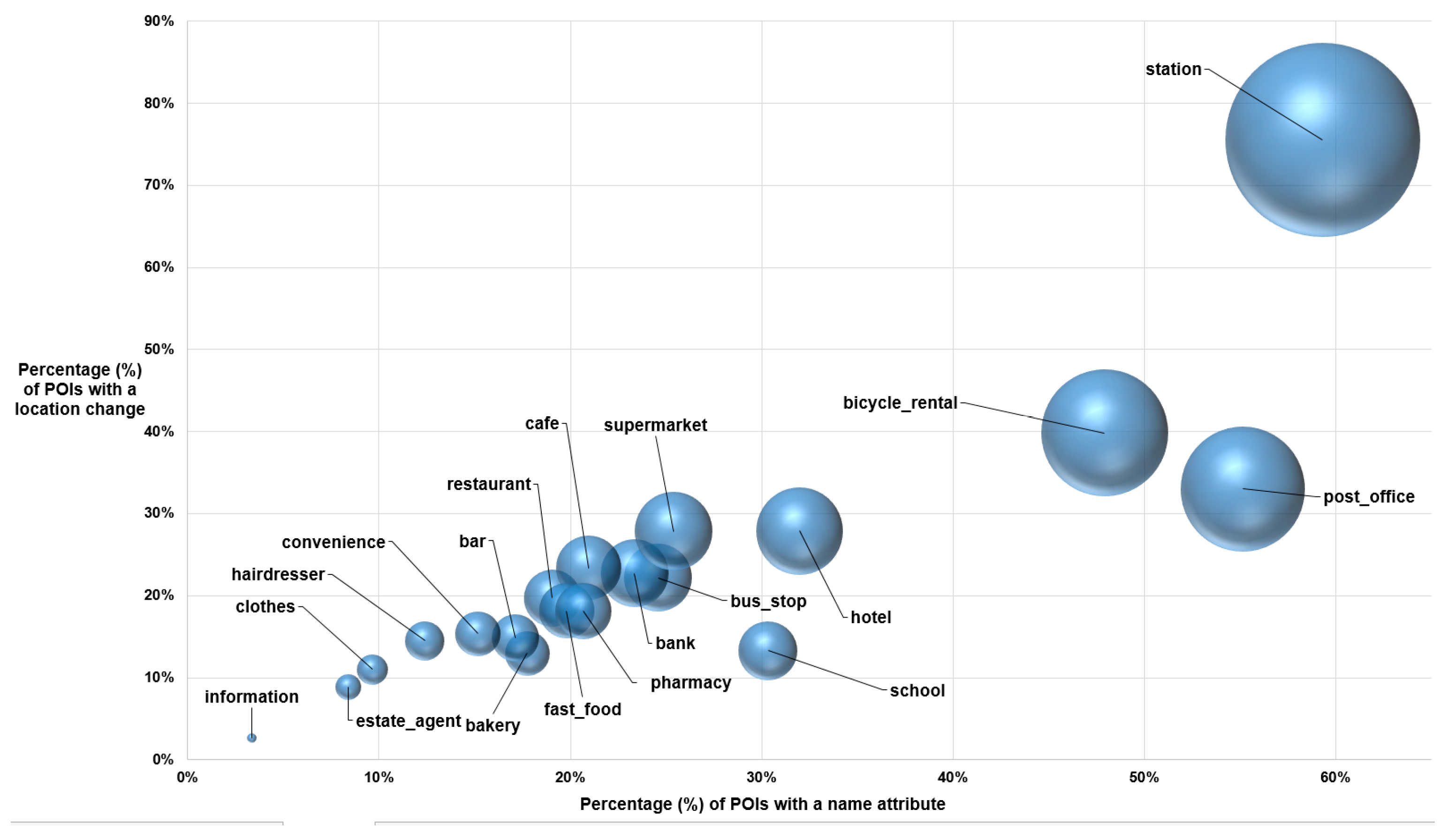
Ijgi 06 00080 g001
Figure 2. Percentage of POIs that had a name (x-axis) and a location (y-axis) change. The size of the bubble corresponds to the intersection of the two changes.
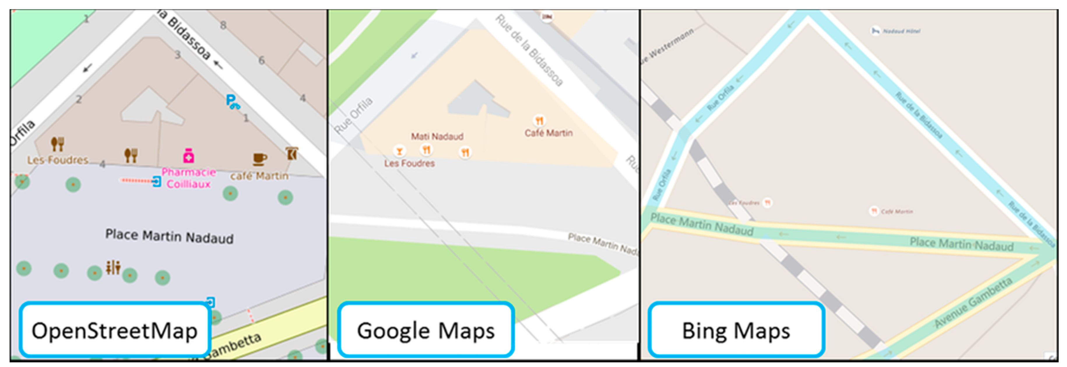
Ijgi 06 00080 g002
Figure 3. Three maps where the POIs are located differently inside the buildings that host them.
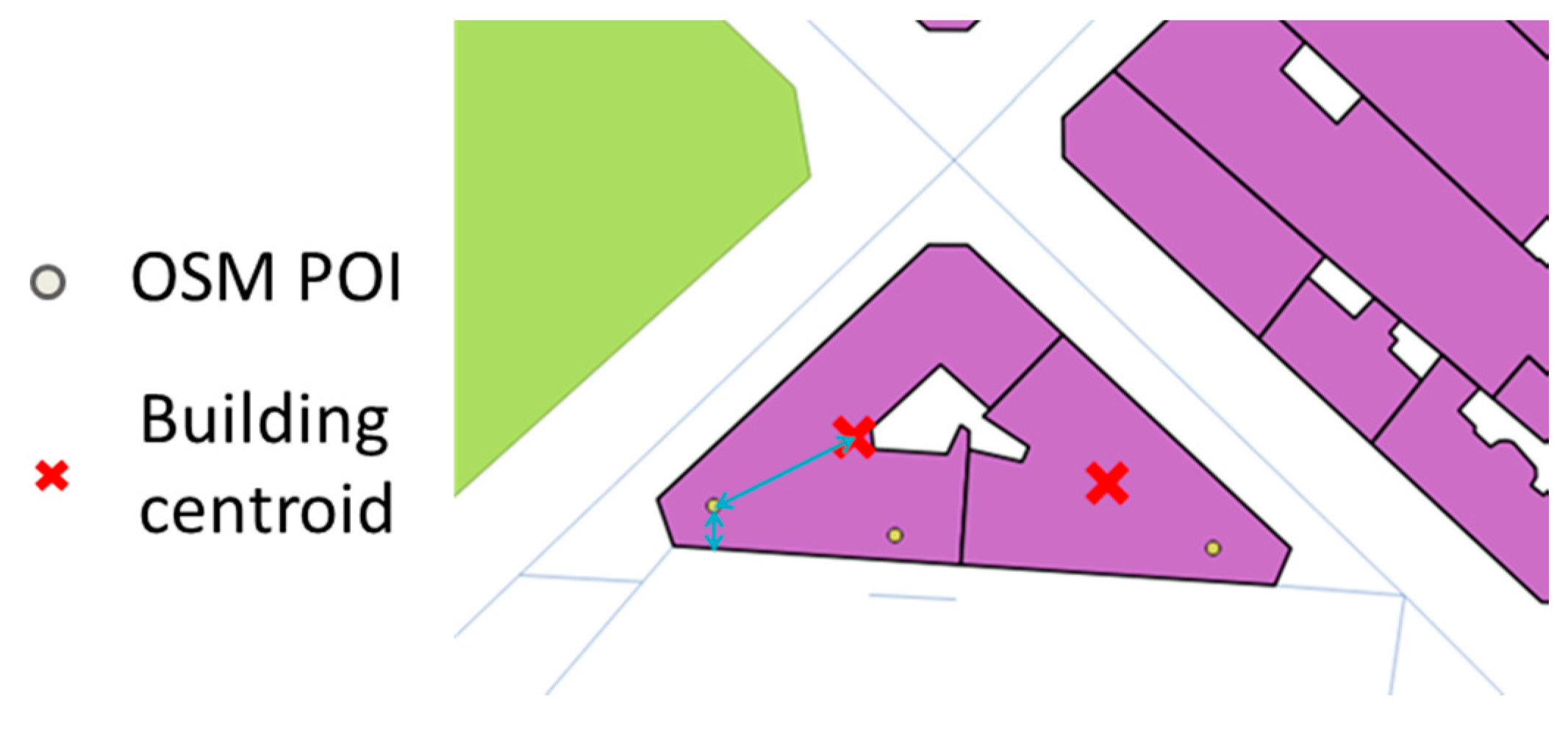
Ijgi 06 00080 g003
Figure 4. Three spatial relations are checked: inside a building, the distance to the building center, and the distance to the nearest boundary as a proxy for an amenity entrance (©OpenStreetMap contributors).
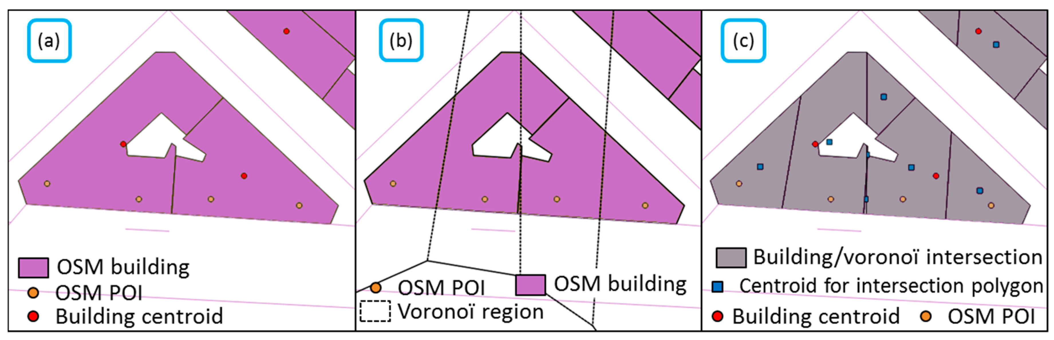
Ijgi 06 00080 g004
Figure 5. (a) One building may cover several amenities so the centroid may be far from the amenity center, (b) using the Voronoï region intersected with the building gives (c) a better approximation of the amenity center (©OpenStreetMap contributors).
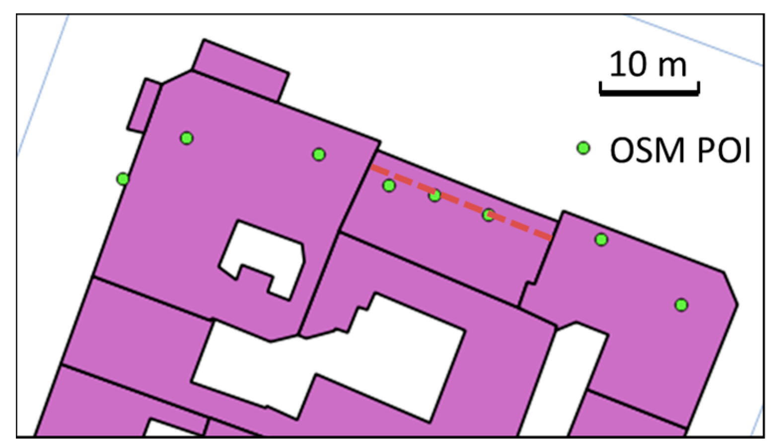
Ijgi 06 00080 g005
Figure 6. Even if there is no unique location for an amenity POI inside a building, consistency in POI location (here points should all be aligned) is better than inconsistency (©OpenStreetMap contributors).
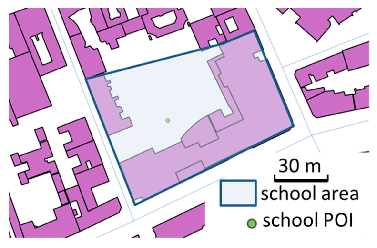
Ijgi 06 00080 g006
Figure 7. A school area, buildings, and a school POI: schools can be composed of several buildings and school yards, so the POI might be located outside a building (©OpenStreetMap contributors).
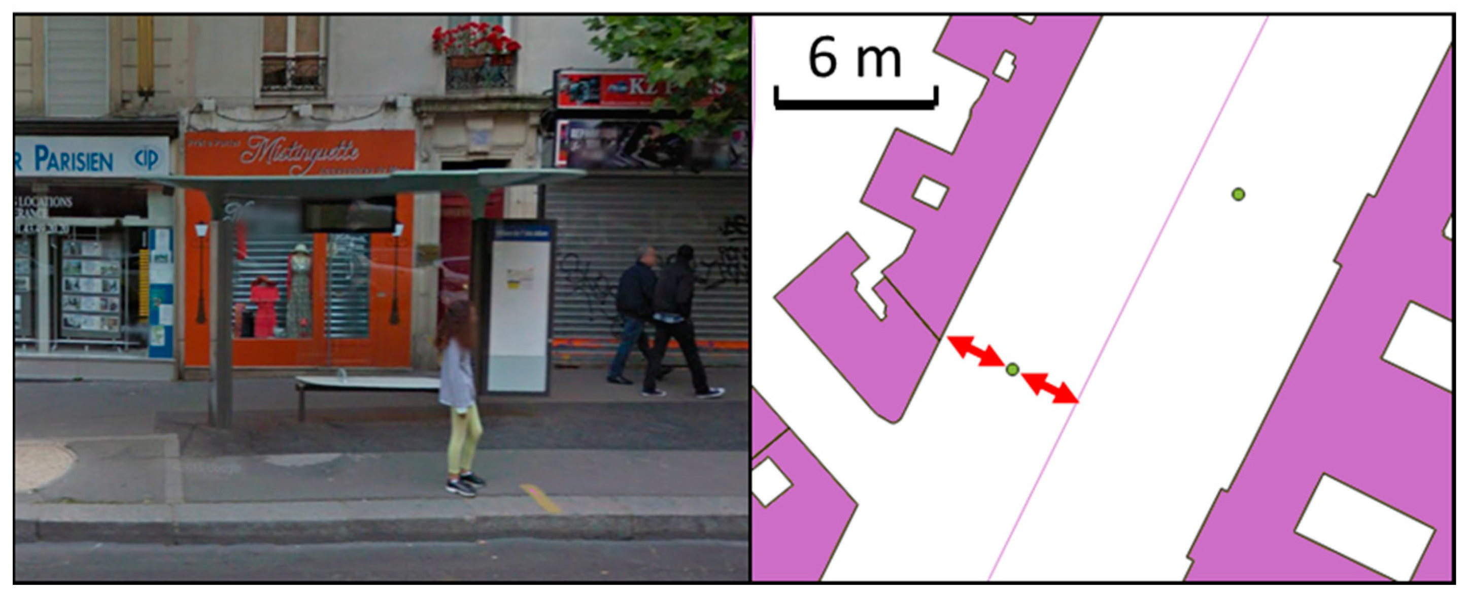
Ijgi 06 00080 g007
Figure 8. Bus stops in Paris are located on the pavement, so should be located far enough from a road centerline and the buildings (©OpenStreetMap contributors).
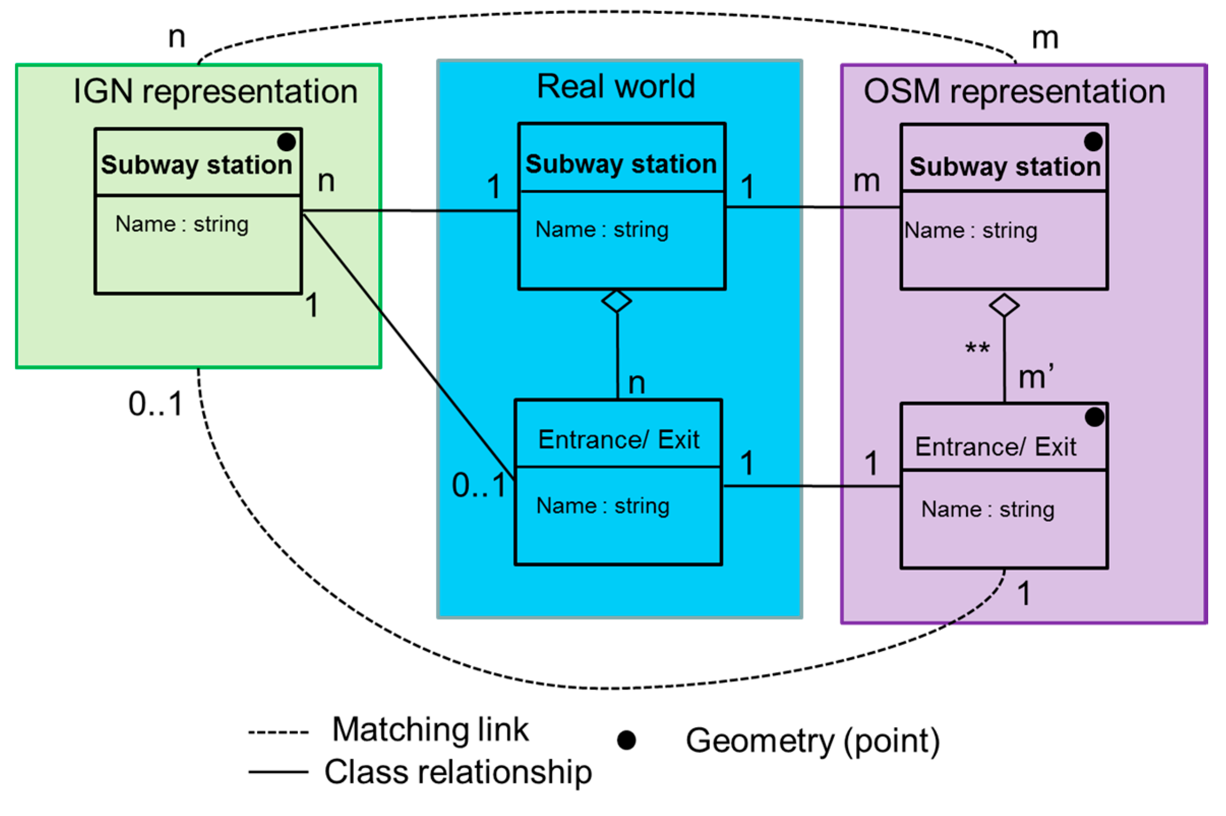
Ijgi 06 00080 g008
Figure 9. Representation of subway stations in OSM and IGN datasets.
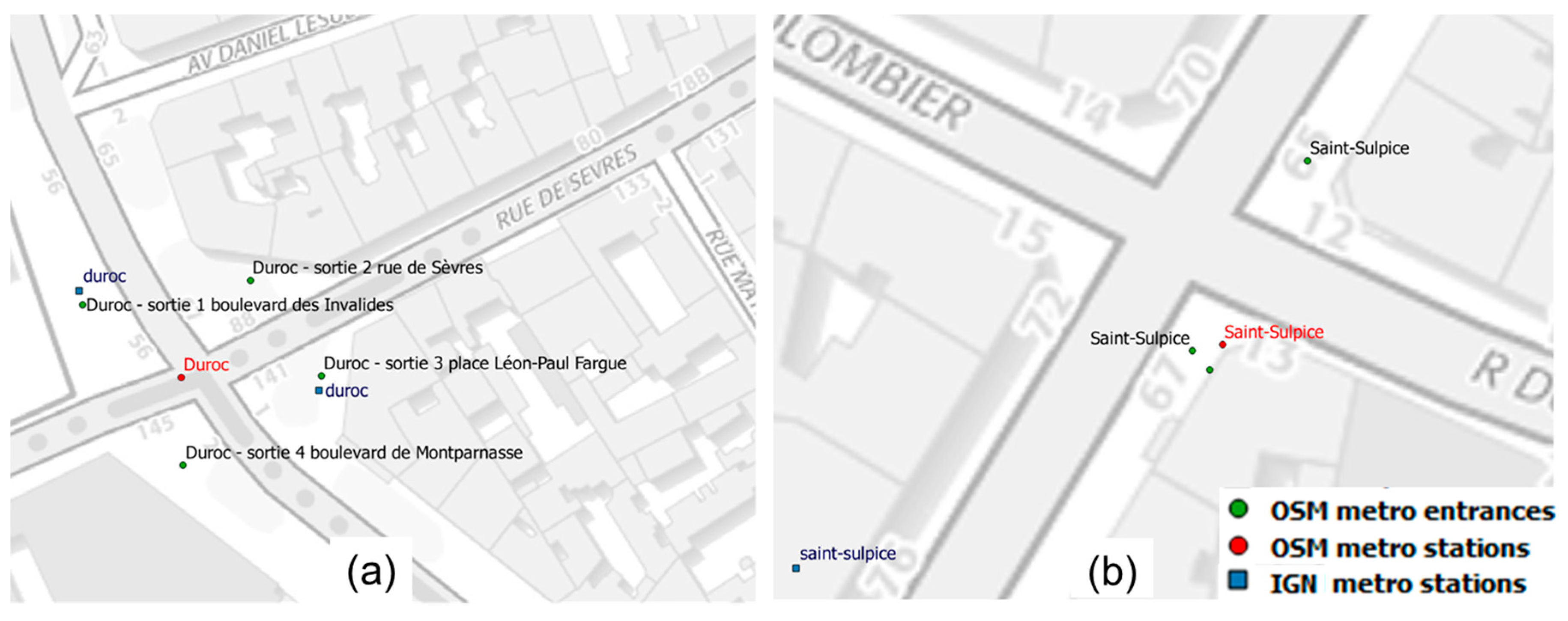
Ijgi 06 00080 g009
Figure 10. Different representations of a subway station: (a) the two station POI in IGN are closer to OSM entrance POIs than to OSM station POI; (b) only one station POI in both datasets but not located at the same place (©OpenStreetMap contributors, ©BDTOPO).
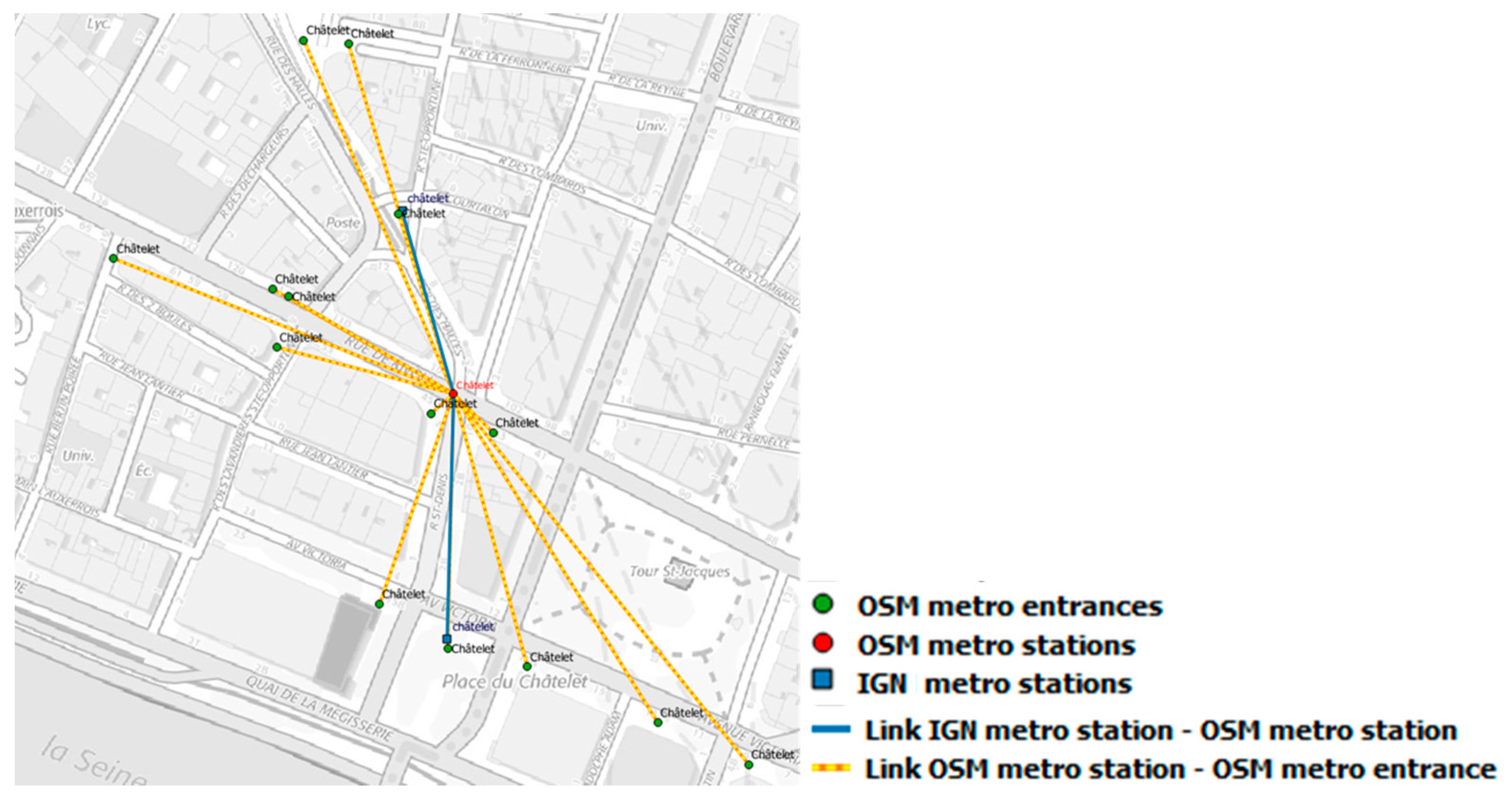
Ijgi 06 00080 g010
Figure 11. Data matching results for Châtelet subway station (©OpenStreetMap contributors, ©BDTOPO).
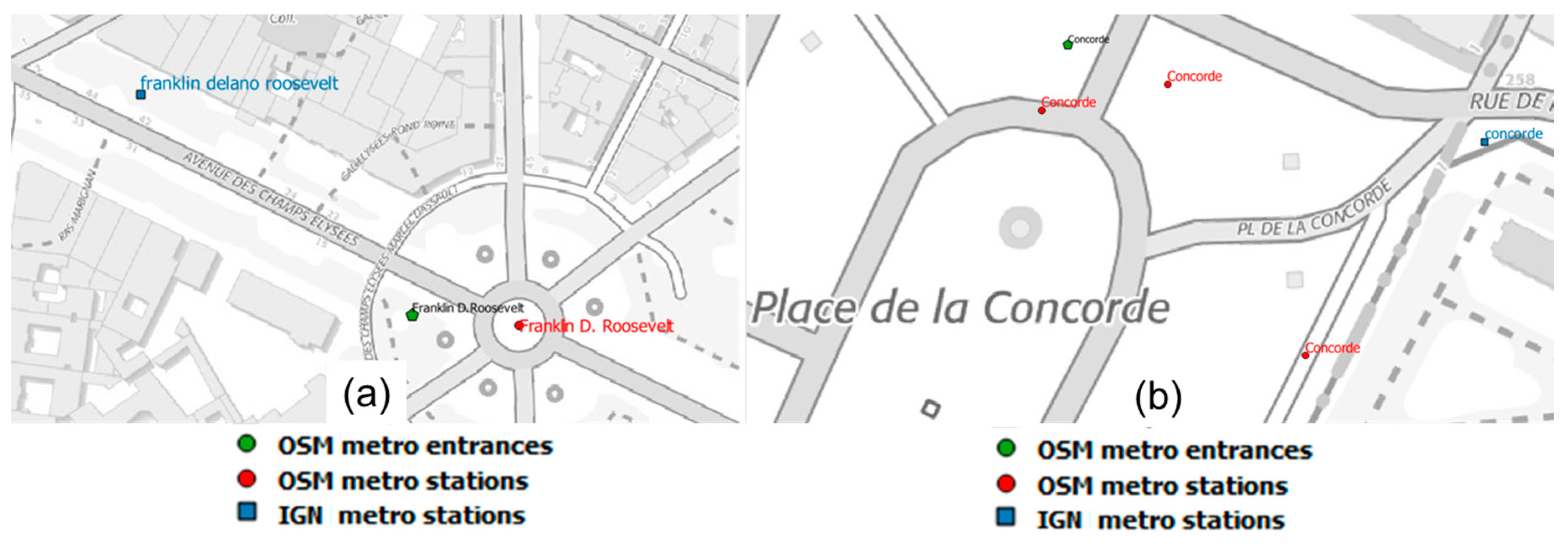
Ijgi 06 00080 g011
Figure 12. Data matching results: (a) wrongly non-matched; (b) correctly non-matched (©OpenStreetMap contributors, ©BDTOPO).
Ijgi 06 00080 g012
Figure 13. Comparison between homologous features: (a) Euclidian distance between IGN and OSM subway stations and (b) Euclidian distance between IGN and OSM subway stations in red and the distance between IGN subway stations and the nearest corresponding OSM subway entrances in green.
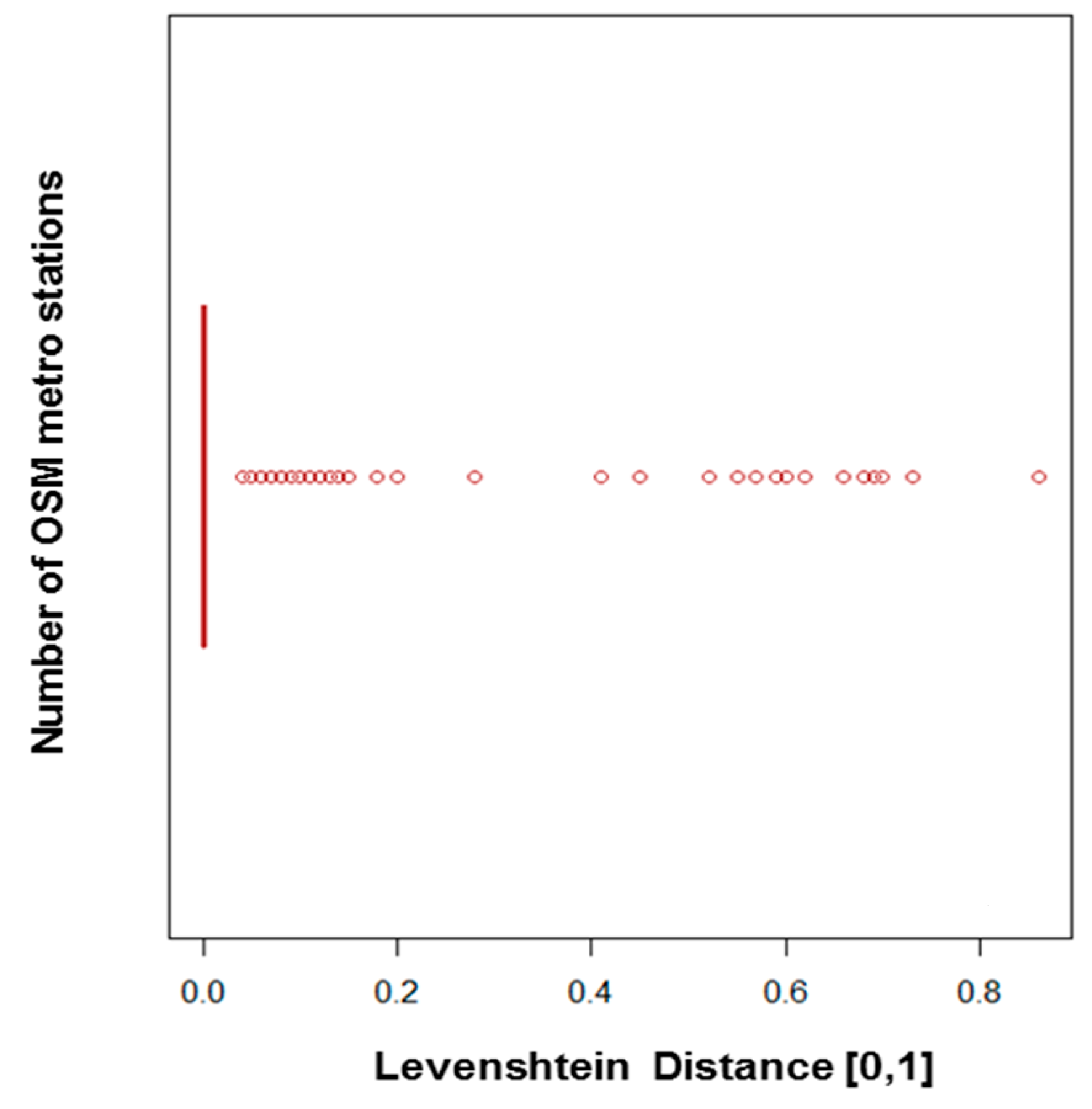
Ijgi 06 00080 g013
Figure 14. Comparison of names of homologous subway stations using the Levenshtein distance.
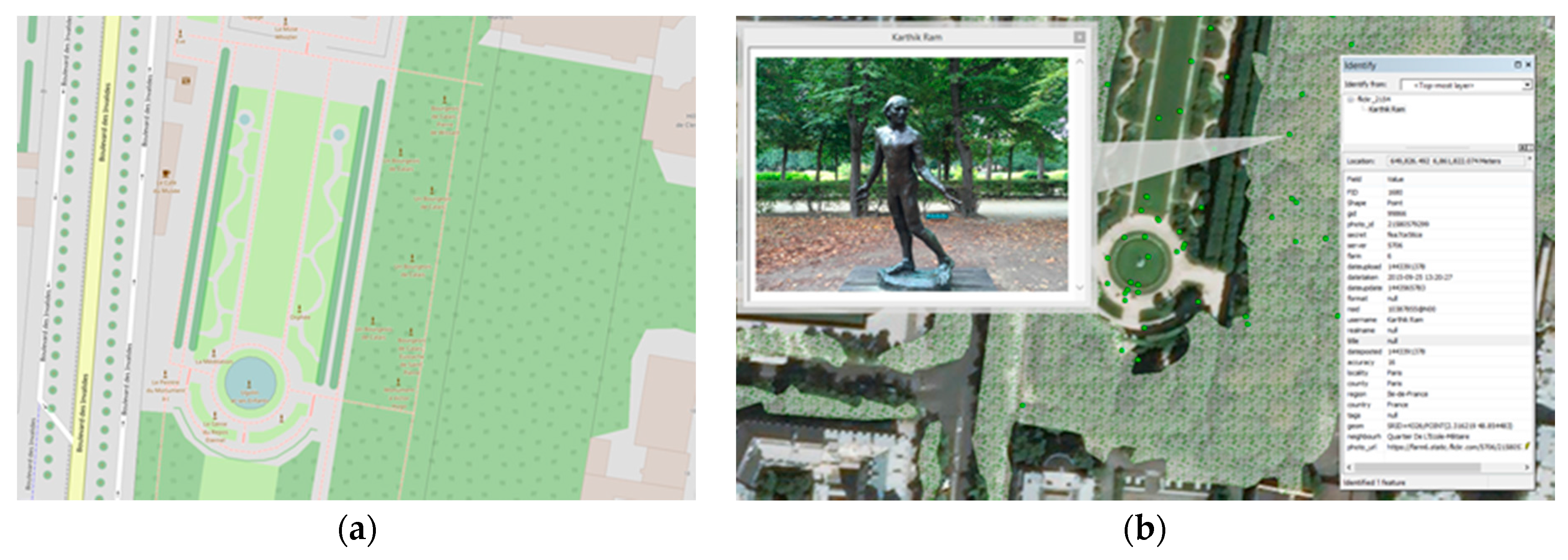
Ijgi 06 00080 g014
Figure 15. The use of Flickr photographs to verify OSM POIs. (a) OSM map for an area in Paris with POIs that are under trees; (b) the same area with the IGN polygons of the wooded areas and the position of geo-tagged Flickr photographs. A Flickr photograph is shown in a pop-up as well as additional attributes provided by the photographer (©OpenStreetMap contributors, ©IGN).
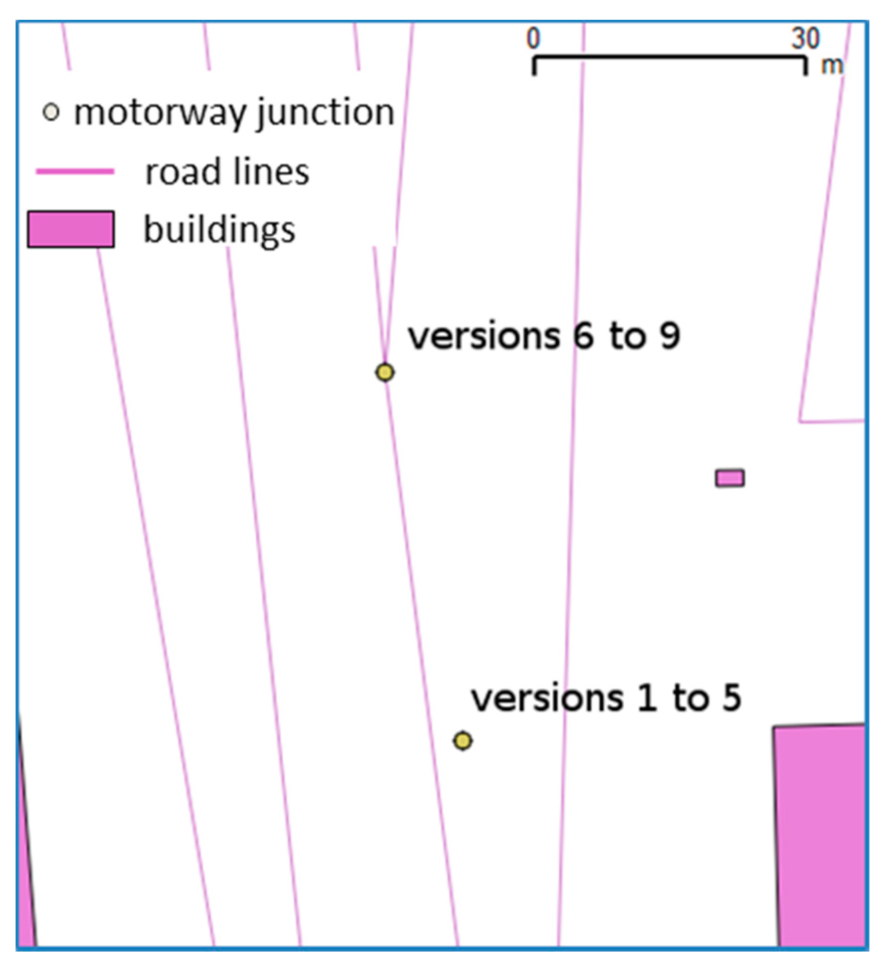
Ijgi 06 00080 g015
Figure 16. The motorway junction is displaced at the intersection of the motorway and the ramp at version 6, where the displacement is large, i.e., greater than 30 m (©OpenStreetMap contributors).
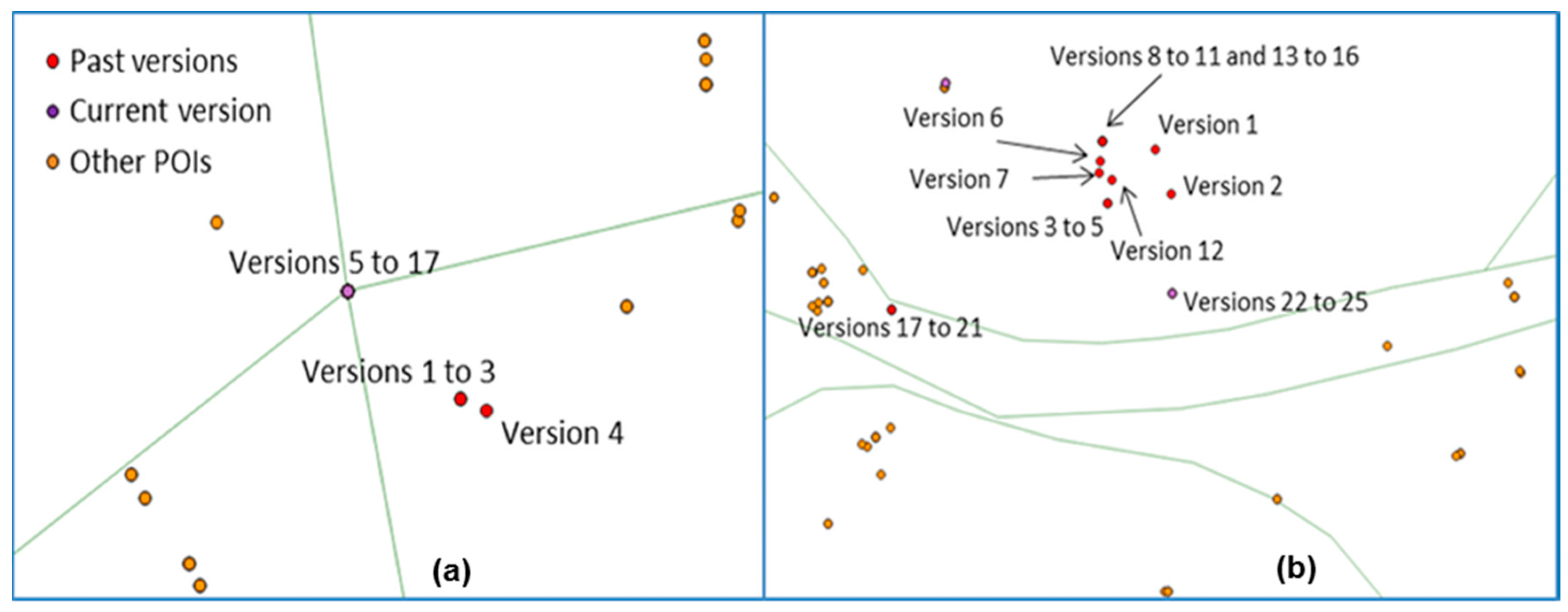
Ijgi 06 00080 g016
Figure 17. Two examples of the evolution of subway station location: (a) the station is put at the intersection of the subway lines in version 5 and then never moves (only tags are then modified); (b) the current version is still wrongly located, and we can see many displacements due to contributor disagreements, as 17 contributors edited this feature (©OpenStreetMap contributors).
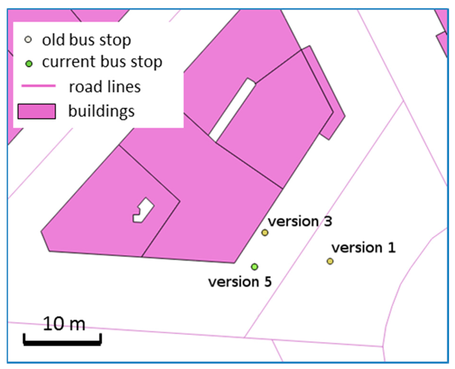
Ijgi 06 00080 g017
Figure 18. Evolution of bus stop location: the bus stop did move between version 1 and 3, but version 5 is just a better placement as version 3 was too close to the building boundary (©OpenStreetMap contributors).
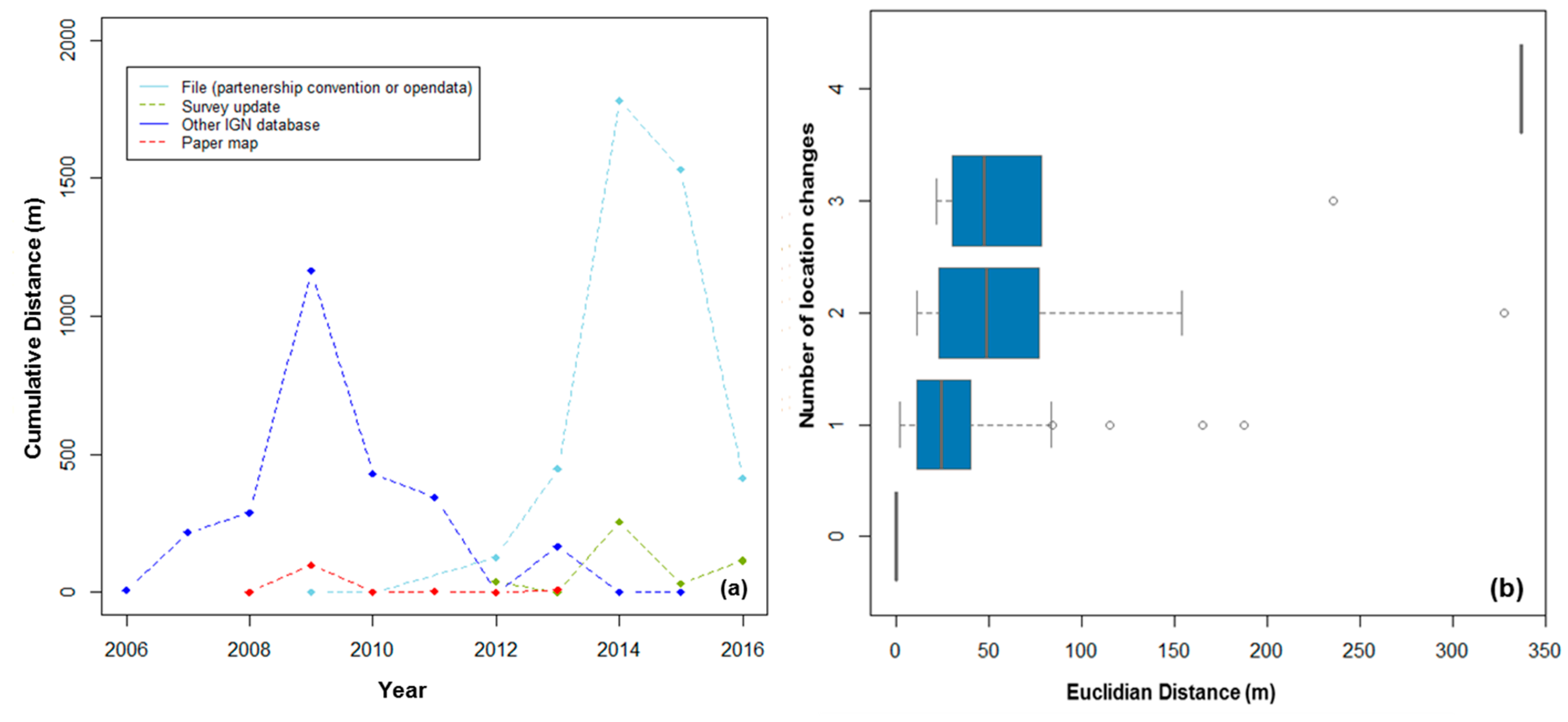
Ijgi 06 00080 g018
Figure 19. Evolution of subway stations in the IGN dataset: (a) sources of change and (b) location changes over time for the Paris region.
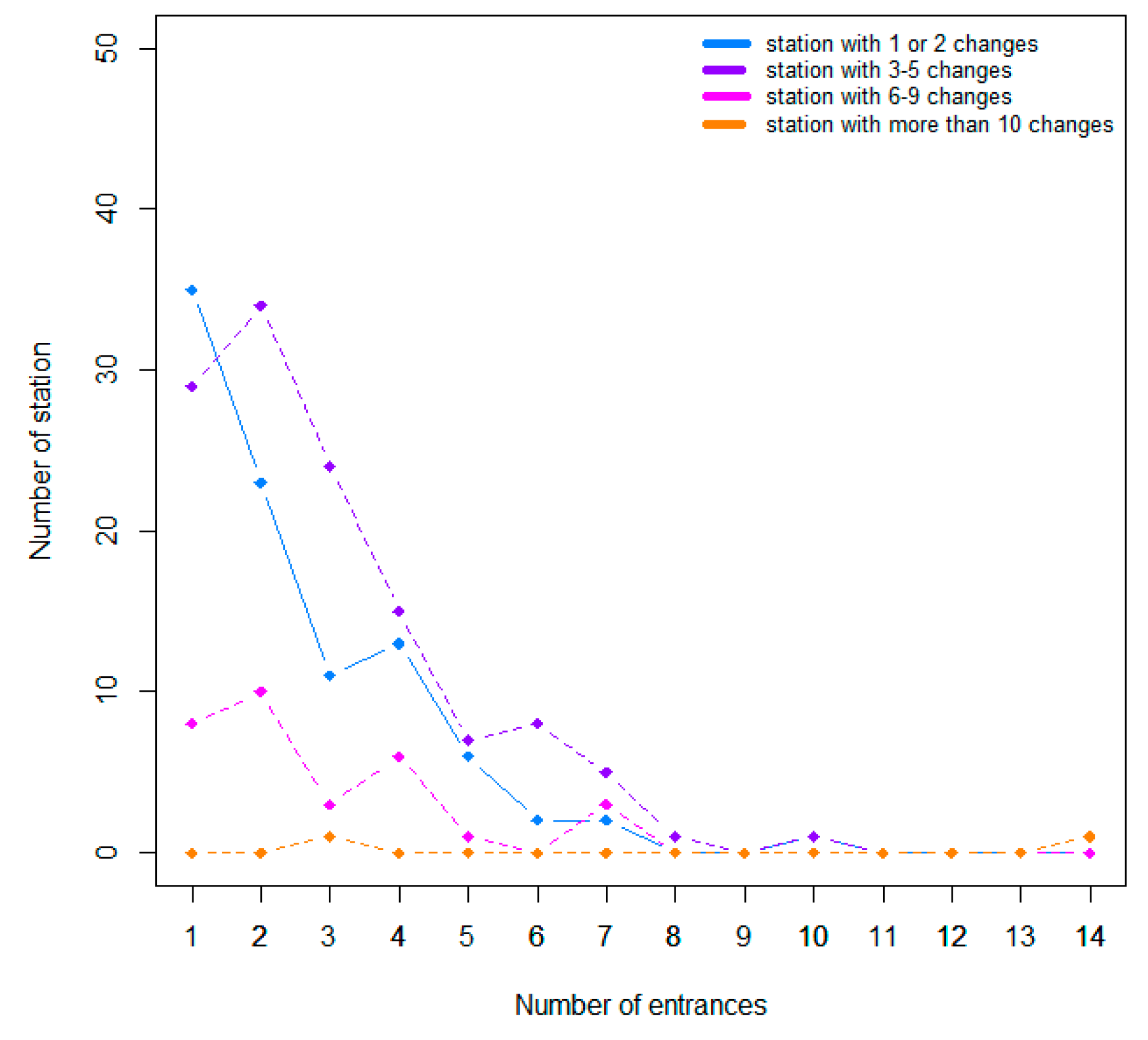
Ijgi 06 00080 g019
Figure 20. Relationship between the number of subway entrances for each subway stations and the number of changes.
Ijgi 06 00080 g020
Table 1. The statistics of the positional movement of the top 10 OSM feature types according to the number of features.
#POI CategoryCountMean Distance (m)SDev. (m)Max Distance (m)
1bus_stop34189.223.6567.0
2restaurant12488.628.7467.4
3station53539.9138.52794.3
4bicycle_rental49913.835.8340.3
5bank4646.419.8349.7
6cafe4526.024.8412.2
7supermarket39311.745.5842.7
8pharmacy3645.714.1198.2
9hotel27414.738.0338.9
10bakery2654.710.9113.1
Table 2. The statistics of the positional movement of the top 10 OSM feature types according to the mean distance (in m) of positional movement.
#POI CategoryCountMean Distance (m)SDev. (m)Max Distance (m)
1station53539.9138.52794.3
2motorway_junction22334.342.7321.5
3fuel18633.775.5659.7
4drinking_water6321.066.0372.6
5hotel27414.738.0338.9
6bicycle_rental49913.835.8340.3
7kindergarten4513.321.3108.3
8school23912.817.2122.7
9supermarket39311.745.5842.7
10post_office23111.123.2250.4
Table 3. Summary of the amenities’ locations consistency in buildings that contain at least three POIs.
% of POIs Outside Buildings (m)Mean Distance to Centroid (DC) (m)SDev. of DC (m)DC with Voronoï (m)Mean Distance to Boundary (DB) (m)SDev. of DB (m)DB with Voronoï (m)
Gift shops012.911.57.722.333.15
Bars, cafes, Restaurants310.810.57.212.32.12.27
Cinemas5.516.918.49.394.94.94.57
Hairdressers1.411.39.57.072.11.22.19
Table 4. Summary of the locations’ consistency of amenities in buildings that contain at least three POIs.
Mean of SDevMedian of SDevMinimum of SDevMaximum of SDev
Distance to center2.991.56076.5
Distance to boundary2.462.15038.5
Table 5. Summary of the ATM locations in relation to building center and boundary.
Mean (m)Median (m)SDev (m)
Distance to center17.61312.9
Distance to boundary1.104.6
Table 6. Summary of the school locations in relation to building/extent center and boundary.
% Outside BuildingsMean Distance to Center (m)Mean Distance to Boundary (m)
Schools with a polygon4031.613.3
Schools without a polygon3019.14.7
Table 7. Summary of the bus stop locations in relation to buildings and road centerlines.
Mean (m)SDev (m)Maximum (m)% Too Close% Too Far
Distance to roads6.22.918.56.80.4
Distance to buildings7.45.8-6.7-
Table 8. Data matching results and evaluation.
Data MatchingNumber of FeaturesPrecisionRecall
IGN subway stations/OSM stations (348 IGN subway stations/704 OSM stations)Matched IGN subway station329 (1 error)99.7%98%
Non-matched IGN subway station9 (2 errors)78%78%
Without decision IGN subway station10--
OSM subway entrances/OSM stations (794 OSM subway entrances/704 OSM stations)Matched OSM subway entrances701100%-
Non-matched OSM subway entrances190%0%
Without decision OSM subway entrances74--
Table 9. Data quality analysis with respect to the observed naming standard for OSM subway entrances.
Name of OSM Subway Entrances Versus Name of Subway Stations
case 1340 OSM subway entrances have a name starting with the corresponding name of the OSM subway station
156 OSM subway entrances have a name partially starting with its corresponding OSM subway station
6 OSM subway stations have a name more detailed than the name of the OSM subway entrances ‘Chaussée d’Antin—La Fayette’ (OSM subway station) versus ‘Chaussée d’Antin’ (OSM subway entrances)
5 OSM subway stations have names strictly integrated into the OSM subway entrances: ‘Denfert-Rochereau’ versus ‘Métropolitain, station Denfert-Rochereau’, ‘Saint-Michel’ versus ‘Quai Saint-Michel (Notre-Dame)’
case 2For an OSM subway station that has at least two corresponding OSM subway entrances, 463 OSM subway entrances have a name contained in the name of the OSM subway station
Among the 463 OSM subway entrances, 306 (66%) have exactly the same name as the corresponding OSM subway station
case 3168 OSM subway entrances contain the word exit. Among those, 22 do not contain the name of the OSM subway station (e.g., ‘Pernéty’ versus ‘Pernety—sortie 2—rue Niepce’. Adding the sign ‘—‘ between the name of the subway station and the word exit has been noticed
142 OSM subway entrances that contain the name of the subway stations follow the standard: Name of the subway station—Exit nn—street xxx (e.g., ‘Bastille—sortie 1—rue de la Roquette’)
4 OSM subway entrances start with the word Exit (e.g., ‘Sortie 3—Rue Goscinny’)
148 OSM subway entrances have a number after the word Exit
Table 10. Change location patterns for subway stations and subway entrances with respect to a reference.
PatternsOSM Subway Station vs. IGN Subway Station (a)IGN Subway Station vs. OSM Subway Station (b)OSM Subway Entrance vs. IGN Subway Station (c)
Without location history00449
Get closer to the reference1096176
Diverging from the reference529260
Disagreement but finally get closer to the reference3597
Disagreement but finally diverge from the reference69647
Disagreement: Get closer and return to the previous location1700
Disagreement: Diverge and return to the previous location1400
Table 11. Evolution of names of OSM subway entrances.
Current Version (T)/523Previous Version Ti+j/258Previous Version Ti+j/64
Case 145811711
Case 238310111
Case 3144173

