Implementation of Algorithm for Satellite-Derived Bathymetry using Open Source GIS and Evaluation for Tsunami Simulation

Abstract

Accurate and high resolution bathymetric data is a necessity for a wide range of coastal oceanographic research topics. Active sensing methods, such as ship-based soundings and Light Detection and Ranging (LiDAR), are expensive and time consuming solutions. Therefore, the significance of Satellite-Derived Bathymetry (SDB) has increased in the last ten years due to the availability of multi-constellation, multi-temporal, and multi-resolution remote sensing data as Open Data. Effective SDB algorithms have been proposed by many authors, but there is no ready-to-use software module available in the Geographical Information System (GIS) environment as yet. Hence, this study implements a Geographically Weighted Regression (GWR) based SDB workflow as a Geographic Resources Analysis Support System (GRASS) GIS module (i.image.bathymetry). Several case studies were carried out to examine the performance of the module in multi-constellation and multi-resolution satellite imageries for different study areas. The results indicate a strong correlation between SDB and reference depth. For instance, case study 1 (Puerto Rico, Northeastern Caribbean Sea) has shown an coefficient of determination (R²) of 0.98 and an Root Mean Square Error (RMSE) of 0.61 m, case study 2 (Iwate, Japan) has shown an R² of 0.94 and an RMSE of 1.50 m, and case study 3 (Miyagi, Japan) has shown an R² of 0.93 and an RMSE of 1.65 m. The reference depths were acquired by using LiDAR for case study 1 and an echo-sounder for case studies 2 and 3. Further, the estimated SDB has been used as one of the inputs for the Australian National University and Geoscience Australia (ANUGA) tsunami simulation model. The tsunami simulation results also show close agreement with post-tsunami survey data. The i.mage.bathymetry module developed as a part of this study is made available as an extension for the Open Source GRASS GIS to facilitate wide use and future improvements.

1. Introduction

Near-shore bathymetry is one of the most important parameters for investigations of coastal processes and hydrodynamic models in coastal areas. As such, the ability to derive near-shore bathymetry using remote sensing techniques is a topic of increasing interest in coastal monitoring and research. The highly dynamic nature of near-shore regions leads to frequent changes in bathymetry that are required to be monitored at periodic intervals, and, hence, the survey should be carried out repetitively, which is almost not practical. Remote sensing is considered an alternative for near-shore bathymetry estimation since a large number of multi-constellation, multi-spectral, and multi-spatial satellite data is available as Open Data. Therefore, near-shore bathymetry based on optical remote sensing has become a cost-effective alternative to Sound Navigation and Ranging (SoNAR) and Light Detection and Ranging (LiDAR) surveys. In order to supplement field based approaches, several optical remote sensing methods have been proposed [1,2,3,4,5].

Satellite-Derived Bathymetry (SDB) models have been purported to retrieve coastal sea bottom reflectance from satellite imagery and effectively utilize this information to generate coastal bathymetry. Researchers have investigated SDB algorithms over the last 30 years and proposed estimation methods falling into categories such as spectral rationing [1,6] and radiative transfer models [7,8,9]. In case of radiative transfer, single spectral band and multispectral band models have been proposed. The single band algorithms assume a constant attenuation coefficient and homogeneous bottom type [8,10,11]. Reliable SDB is possible when the water is clear and when water quality and bottom types are homogeneous. When such conditions are satisfied, single band water depth models can provide a reasonable estimate of depth. Nonetheless, coastal water environments rarely offer such ideal conditions. Therefore, radiative transfer models using linear regression of multispectral bands [7,9,12] have yielded good results.

In order to improve the efficacy of multispectral models in SDB estimation, many statistical approaches have been adopted [13]. Recently, the Geographically Weighted Regression (GWR) model has been successfully applied as a predictive weighted linear regression model [14,15,16,17,18] in various fields. Further, [19,20] have successfully used a GWR model for improved SDB estimation. However, until now, no software module has been proposed to automate the SDB procedures that use a GWR model. Therefore, we have implemented a new Open Source Geographic Resources Analysis Support System (GRASS) Geographic Information System (GIS) module termed i.image.bathymetry to automate the bathymetry estimation from multispectral images. Since i.image.bathymetry has been entirely implemented using a Free and Open Source GIS framework, it can be easily applied in other areas without the need to invest resources for software and can also be further improved in the future. Study further aims to generate an Integrated Coastal Relief Model (ICRM) by combining multi-resolution topographic and bathymetry data. The ICRM is used to evaluate a practical application scenario of the SDB in tsunami simulation.

2. System Environment

The i.image.bathymetry module to estimate SDB has been developed in GRASS GIS Version 7 [21]. GRASS GIS is a robust Open Source GIS widely used in academia, commercial settings, and governmental agencies. A powerful feature of GRASS is the availability of the Python scripting library, which is used to implement several customizable modules for geoprocessing. In addition, GRASS GIS also provides access to R Project for Statistical Computing (R) through numerous packages for geospatial and geostatistical analysis. The availability of the rgrass7 package as an interface between GRASS and R is one of the reasons to choose GRASS GIS for the implementation of i.image.bathymetry. The effectiveness of GRASS GIS in analyzing big data, its ease in implementing Python modules, and the deployment parallel computing platform were also considered.

2.1. GRASS Python Scripting Library

Python [22], a widely used programming language provides a powerful scripting environment in GRASS GIS. It enables users to efficiently exploit the capabilities of GRASS GIS software for developing new modules and extensions. In this study, the GRASS Python scripting library [23] has been used to combine multiple modules and functions from GRASS and R to implement the SDB algorithm.

2.2. R Packages

R [24] is an Open Source statistical computing environment that provides several spatial analysis packages and functions. rgrass7 [25] provides an interface between GRASS GIS 7 and R. The package provides access to all GRASS commands from the R command line. The rgrass7 package can be used to import/export data from GRASS to R and vice versa. The rgrass7 package is only available beyond R Version 3.1; therefore, that should be installed in order to use the i.image.bathymetry module. Another library, data.table, is used to manage the spatial data frame of the raster data in R. GWmodel [26] is a collection of functions, which is considered a particular branch of spatial statistics, called geographical weighted models, and is used to deploy the GWR functionality.

3. Implementation of SDB Model as GRASS GIS Module

The i.image.bathymetry is a collection of many existing GRASS GIS and R modules and new functions. The main functionalities of the module are (1) delineating water region; (2) atmospheric and water corrections; (3) GWR. An atmospheric and water corrections algorithm was adopted from previous authors and improvements have been made in terms of band selection [9,12]. Geometrically and radiometrically corrected spectral bands of any optical multispectral remote sensing data can be used to estimate SDB from the suitable coastal region. In the flowchart (Figure 1), the dotted box shows the required spectral bands, optional spectral bands, and other input data such as calibration depth points (as vector point type) and tide height. The spectral bands in the green, red, Near-infrared (NIR), and Short Wave Infrared (SWIR) wavelengths are mandatory inputs. Other spectral bands available in the visible domain can be supplemented as additional bands depending upon the satellite sensor.

3.1. Delineation of Water Region

The first step in the processing chain of i.image.bathymetry is the delineation of the water region. A rule based combination of the Normalized Difference Vegetation Index (NDVI) and a band ratio between the green and infrared bands were used for effective delineation. A band ratio of greater than or equal to 1 was classified as water and less than 1 was classified as land [11]. A masked water region has been used for further processing. NDVI has been used to remove the cloud, ice, etc., from the water region. GRASS GIS module r.mapcalc is used for these calculations to delineate water pixels effectively (Step 1 in Figure 1).

3.2. Tide Correction

In spite of the availability of numerous satellite images, very rarely satellite images are acquired at the time of zero tide. Therefore, the i.image.bathymetry module has an option to provide a tide height specific to the time of satellite image capture and to carry out tide correction (step 2 in Figure 1). The tide height at the time of image acquisition can be provided and used to correct the calibration depth. If the tide at the time of satellite image acquisition is lower than zero, a negative value can be provided as tide height. The user provided tide height value will be incremented to calibration depth, and, hence, the tide height at the time of image acquisition and the calibration depth would be synchronized. This option can also be used when the same calibration depth is used in multi-temporal SDB estimation.

3.3. Atmospheric and Water Corrections

The radiance observed by a satellite sensor on shallow water basically consists of four components, namely, atmospheric scattering, surface reflection, in-water volume scattering, and bottom reflection components [20]. Many authors have proposed various algorithms for atmospheric and water corrections [6,8,10]. Among them, some authors [12] have suggested to perform atmospheric correction prior to the water corrections. Nonetheless, this study adopted a more refined way of retrieving bottom reflectance originally proposed by [9] by removing atmospheric, water surface, and water column components. The observed spectral radiance L(λ) is a function of the wavelength and can be expressed as shown below;

$$L\left(\lambda \right)=V\left(\lambda \right)+B\left(\lambda \right)+S\left(\lambda \right)+A\left(\lambda \right)$$

(1)

where V(λ) is the in-water volume scattering, B(λ) is the bottom reflectance, S(λ) is the water surface reflectance, and A(λ) is the atmospheric scattering [20].

In deep water, even a short wavelength band does not include a bottom reflectance component and can be considered to correspond to pixels of infinite depth (L(λ_∞)_i). The target of interest in SDB is the shallow-water area that contains bottom reflectance, which can be transformed to depth. Delineation of deep water pixels is relatively simple by visual interpretation, but, in this case, calibration depth points have been used to demarcate the shallow water pixels or the area of interest. Pixels that have lower reflectance than the minimum reflectance value of the shallow water region will be considered deep water pixels. This assumption is based on the fact that deep water pixels of any visible spectral band show lower reflectance than shallow water pixels. Spectral radiance of a deep water region is mainly a contribution of atmospheric scattering, surface reflectance, and in-water volume scattering. Therefore, one can expect a correlation between the visible band and the NIR band. The estimation of regression coefficients using the visible band and the NIR band in deep water regions is shown in Equation (2) below [12]. The calculation of regression coefficients is done using GRASS GIS module r.regression.line.

$$L{({\lambda }_{\infty })}_i= {\alpha }_{0i}+ {\alpha }_{1i} (L{\left({\lambda }_{\infty }\right)}_{NIR})$$

(2)

A logarithmically transformed Equation (3) was proposed by [1] for atmospheric and water corrections.

$$X{\left(\lambda \right)}_i = \log (L{\left(\lambda \right)}_i – mean (L\left({\lambda }_{\infty }{)}_i\right)$$

(3)

where X(λ)_i is the transformed radiance, L(λ)_i is the spectral radiance of the ith band over a shallow water region, and (L(λ_∞)_i) is the spectral radiance of the ith band in deep water region. The regression coefficients (${\alpha }_{0i}, {\alpha }_{1i}$) derived from deep water pixels by the regression between the respected spectral band and the NIR band (Equation (2)) are used for atmospheric and water corrections of a shallow water region or area of interest. The radiance of the deep water pixel (L(λ_∞)_i) from Equation (2) can be substituted into Equation (3) to derive a transformed radiance as shown below:

$$X{\left(\lambda \right)}_i=log(L{\left(\lambda \right)}_i-({\alpha }_{0i}+ {\alpha }_{1i} (L{\left(\lambda \right)}_{NIR})))$$

(4)

To compute Equation (4), first of all, the working region in GRASS GIS should be changed to the shallow water region or area of interest. Subsequently, estimated values of α_0i and α_1i for the deep-water pixels are used to calculate the transformed (X(λ)_i) of shallow water pixels for the respective bands using the r.mapcalc function (step 3 in Figure 1).

3.4. Geographical Weighted Regression

The GWR model is a weighted regression model that computes β-coefficients for each pixel [16]. In GWR models, the term bandwidth denotes the radius of the kernel window. In the case of the Bi-square function (Equation (5)), decay of weighting would be applied only if the distance from the current pixel is less than the bandwidth, else the assigned weight will be zero. On the other hand, the continuous Gaussian function (Equation (6)) gives the fractional decay of weights according to the proximity of a pixel to the current pixel, even if the distance from the current pixel is greater than the bandwidth.

$$w_p={(1-{\left(d/bw\right)}^2)}^2$$

(5)

$$w_p= exp(-0.5 * \left(d/bw{)}^2\right)$$

(6)

Where, bw is the bandwidth, d is the distance from a pixel to the current pixel, and w_p is the weight assigned to a pixel. In the i.image.bathymetry module, the Gaussian kernel is default; otherwise the user can choose the bi-square kernel by using a -b flag as shown in the Figure 1. Prior knowledge is required in order to choose the appropriate kernel type. [20] has discussed in detail the selection of the appropriate kernel in terms of the surface to be estimated and the distribution of calibration points.

3.4.1. Fixed-GWR

In GWR, the selected bandwidth determines the spatial coverage of the local kernel, and assigning the appropriate bandwidth is critical. There are two ways of assigning bandwidth; one is fixed bandwidth (Fixed-GWR) and the other is adaptive bandwidth. In case of Fixed-GWR, the size of the kernel is the same all over the working domain. Therefore, Fixed-GWR treats the entire region uniformly irrespective of the distribution of calibration depth points. The Fixed-GWR model is less computationally intensive and less memory consuming as compared to an adaptive GWR (A-GWR) model. Consequently, the Fixed-GWR model is available in many software packages, and therefore it is easy to apply. In GRASS GIS 7, the module r.gwr computes the Fixed-GWR and A-GWR with bi-square, Gaussian, and exponential kernels. The i.image.bathymetry module has adopted the r.gwr module to process Fixed-GWR by selecting a system generated optimal bandwidth. The corrected spectral bands are used as independent variables and calibration depth as the dependent variable to calculate Fixed-GWR (step 4a in Figure 1). A flag (-f) has been implemented in order to carry out depth estimation using Fixed-GWR (Figure 1).

3.4.2. Adaptive-GWR

In an A-GWR model, the size of the kernel is set by considering the density of calibration points in a local neighborhood. The size of the kernel is smaller when calibration points are denser, and the size of the kernel increases when calibration points are sparse. Previous research [18] has demonstrated that adaptive bandwidth performs relatively better, particularly in the case of randomly distributed calibration points. The module called GWmodel, available in R, has been used to calculate A-GWR. Corrected spectral bands (step 3 in Figure 1) are imported to R using the library rgrass7, and these spectral bands are further converted to a spatial data frame using the library data.table (step 4b in Figure 1). A spatial data frame of spectral bands is used as the independent variable and reference depth is used as the dependent variable to compute A-GWR using the library GWmodel. In GWmodel, the function called bw.gwr is used to calculate the optimal bandwidth. In GWmodel, the optimal bandwidth is determined using a cross-validation approach in which the validation scores are minimized [16,27,28]. An A-GWR model is slower and needs more memory than a Fixed-GWR model. However, because of its better performance, i.image.bathymetry by default uses an A-GWR model. If the particular system not able to run the A-GWR model due to low memory, a Fixed-GWR will be used to estimate SDB (step 4b in Figure 1).

4. Validation of Implemented SDB Algorithm

Several tests have been carried out with various satellite imageries to evaluate the performance of i.image.bathymetry to estimate SDB. Here, we present three case studies carried out in Puerto Rico and parts of the Iwate and Miyagi Prefectures.

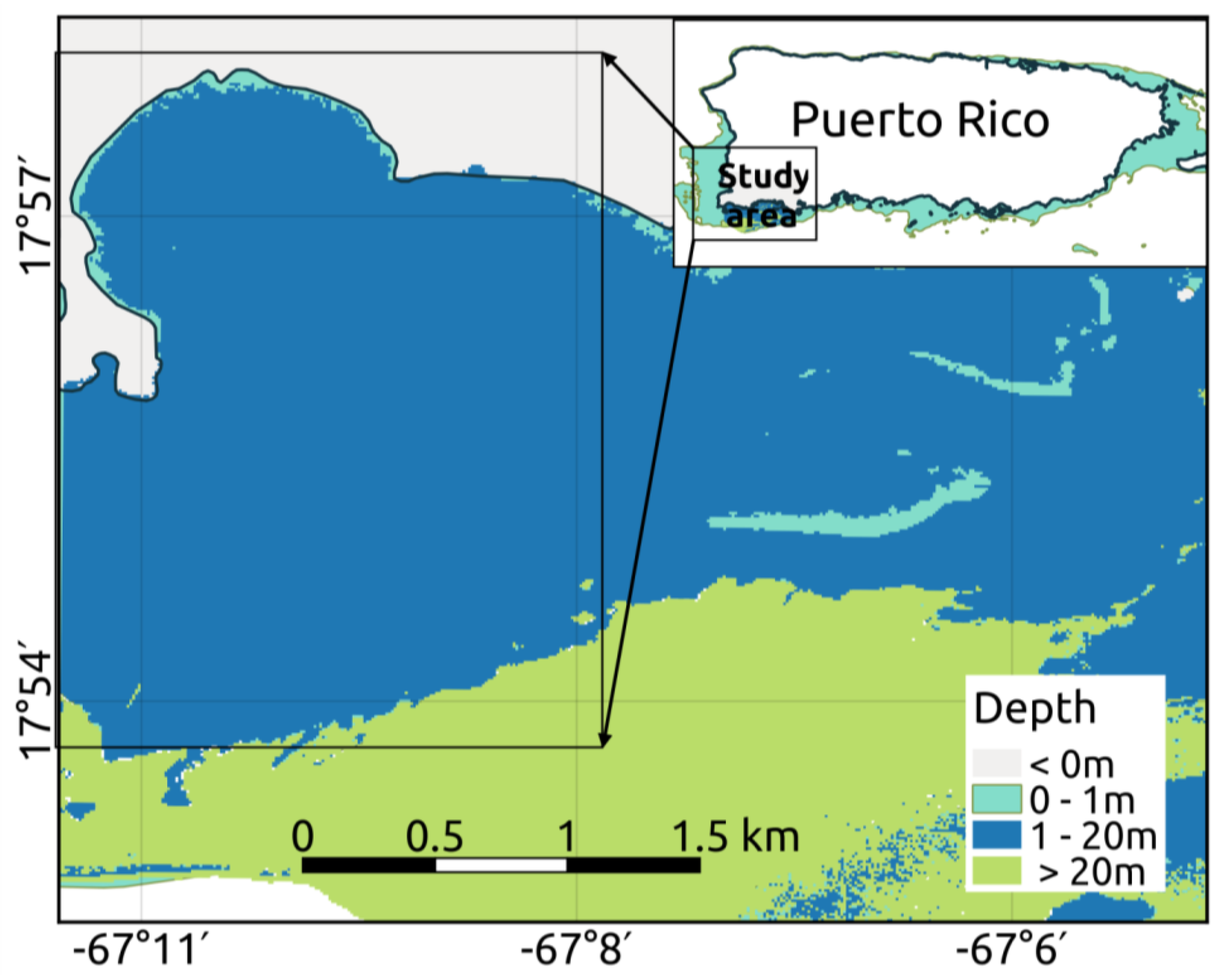
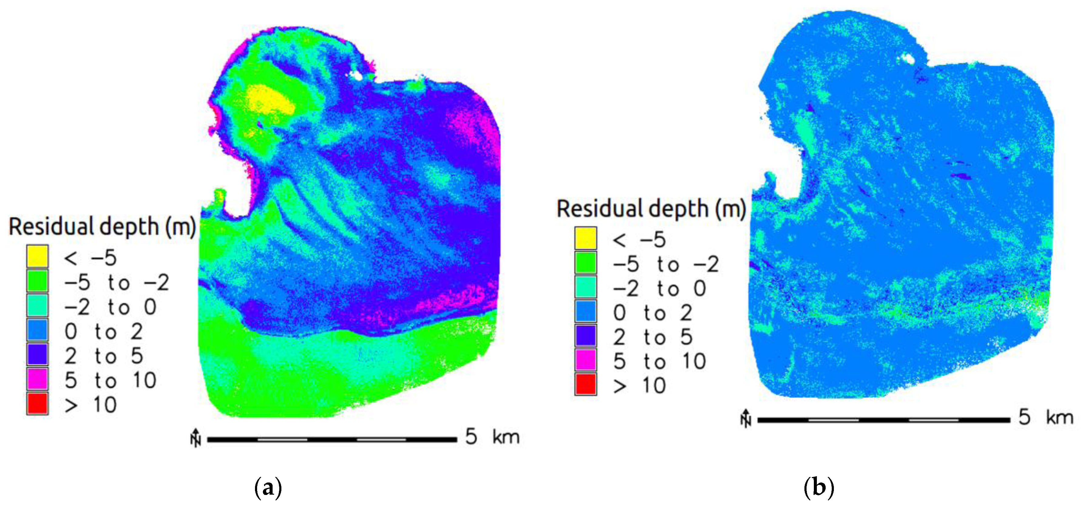
4.1. Puerto Rico, Northeastern Caribbean Sea

The study area is shown in Figure 2 and geographically covers 17°54′ N–17°58′ N and 67°08′ E–67°12′ E, about 40 km² along a 10 km coastal stretch off Puerto Rico. The Puerto Rico coastal stretch was selected as a study area for two reasons; one of them is the availability of open high resolution LiDAR data provided by National Oceanic and Atmospheric Administration (NOAA). Secondly, clear water conditions observed in the region could afford better estimation. LiDAR bathymetric data provided by NOAA were acquired using a Laser Airborne Depth Sounder (LADS) Mk II Airborne System, which surveyed between 7 April 2006 to 15 May 2006. The final product imagery (16-bit Geotiff image) has been produced at 4 m × 4 m bathymetry surface [29].

Sentinel-2 Multi Spectral Instrument (MSI) high spatial and radiometric resolution data were collected on 25 December, 2015. Compared to other satellite imageries, Sentinel-2 have a spatial resolution that varies from 10 m to 60 m for multispectral bands and radiometric resolution quantized over a 12-bit dynamic range and rescaled to 16-bit. In addition to that, Sentinel-2 provides several red edge bands that can be effectively used as additional bands for SDB estimation. The availability of the SWIR band (1.53–1.68 μm) is another significant feature of Sentinel-2, which can be used for atmospheric and water corrections. In this study, bi-linear interpolation has been carried out to resample the pixels of the SWIR band from 20 m to 10 m. One 20 m pixel can be divided in to four 10 m pixels; the value of first pixel was assigned as the original value of the 20 m pixel, and the values of other three pixels were interpolated using Equation (7). This interpolation method has been carried out for all 20 m pixels to keep the original value for the first pixel of the four interpolated 10 m pixels.

$$Z= Z_1\left(1-t\right)\left(1-u\right)+ Z_{2}u\left(1-t\right)+ Z_{3}t\left(1-u\right)+ Z_{4}ut$$

(7)

where, Z is the value of the pixel and x, y is the coordinates of Z in a matrix, respectively; Z₁, Z₂, Z₃, and Z₄ are the neighboring pixels which are used for the calculation and (x₁, y₁), (x₁, y₂), (x₂, y₁), and (x₂, y₂) are the coordinates, respectively. t and u are the slopes between these coordinates, which can be written as (x − x₁)/(x₂ − x₁) and (y − y₁)/(y₂ − y₁), respectively.

All the available bands in the visible domain and the Near-infrared (NIR) band were used for Satellite-Derived Bathymetry (SDB) estimation, as shown in

Table 1. Characteristics of data used.

Data	Date	Res.(m)	Estimation Bands	Correction Band
Landsat-8	31 October 2014	30	0.43–0.45 μm (coastal)	1.57–1.65 μm (SWIR)
		30	0.45–0.51 μm (blue)
		30	0.53–0.59 μm (green)
		30	0.64–0.67 μm (red)
		30	0.85–0.88 μm (NIR)
Sentinel-2	25 December 2015	10	0.44–0.53 μm (blue)	1.53–1.68 μm (SWIR)
		10	0.53–0.58 μm (green)
		10	0.64–0.68 μm (red)
		20	0.69–0.71 μm (Red-edge)
		20	0.73–0.74 μm (Red-edge)
		10	0.76–0.90 μm (NIR)
ASTER	10 September 2010	15	0.52–0.60 μm (green)	0.76–0.86 μm (NIR)
		15	0.63–0.69 μm (red)

. Tide height during satellite image acquisition was nearly zero; therefore no tide correction was applied. The estimation has been carried out using 1260 depth points as the dependent variables, and another 2000 depth points were used to validate the results. Both calibration and validation depth points ranged from 0 to 20 m. First of all, a global model [20] has been used to estimate SDB, and the results show reliable accuracy in terms of correlation coefficient (R) of 0.86, coefficient of determination (R²) of 0.74 and Root Mean Square Error (RMSE) of (2.53 m) as shown in

Table 2. Comparison of accuracy of SDBs generated by global model and GWR model case studies 1, 2, and 3.

Case Studies	Global Model			GWR Model
	R	R2	RMSE (m)	R	R2	RMSE (m)
Puerto Rico	0.86	0.74	2.53	0.99	0.98	0.61
Iwate	0.80	0.65	3.59	0.97	0.94	1.50
Miyagi	0.78	0.61	3.18	0.93	0.87	1.65

. Nonetheless, a detailed investigation using a residual depth map (Figure 3a) indicates that spatial heterogeneity was not effectively addressed by a global model. Therefore, further study used GWR based models in order to exploit spatial auto-correlation by addressing the spatial heterogeneity. Various weighting functions in fixed bandwidth GWR (Fixed-GWR) and adaptive GWR (A-GWR) were tested. Among different options attempted, A-GWR using bi-square kernel produced high accuracy SDB. Results were evaluated in terms of R (0.99), R² (0.98,) and RMSE (0.61 m). Figure 3b clearly demonstrates the efficacy of a GWR based model in addressing the heterogeneity due to bottom types or water conditions.

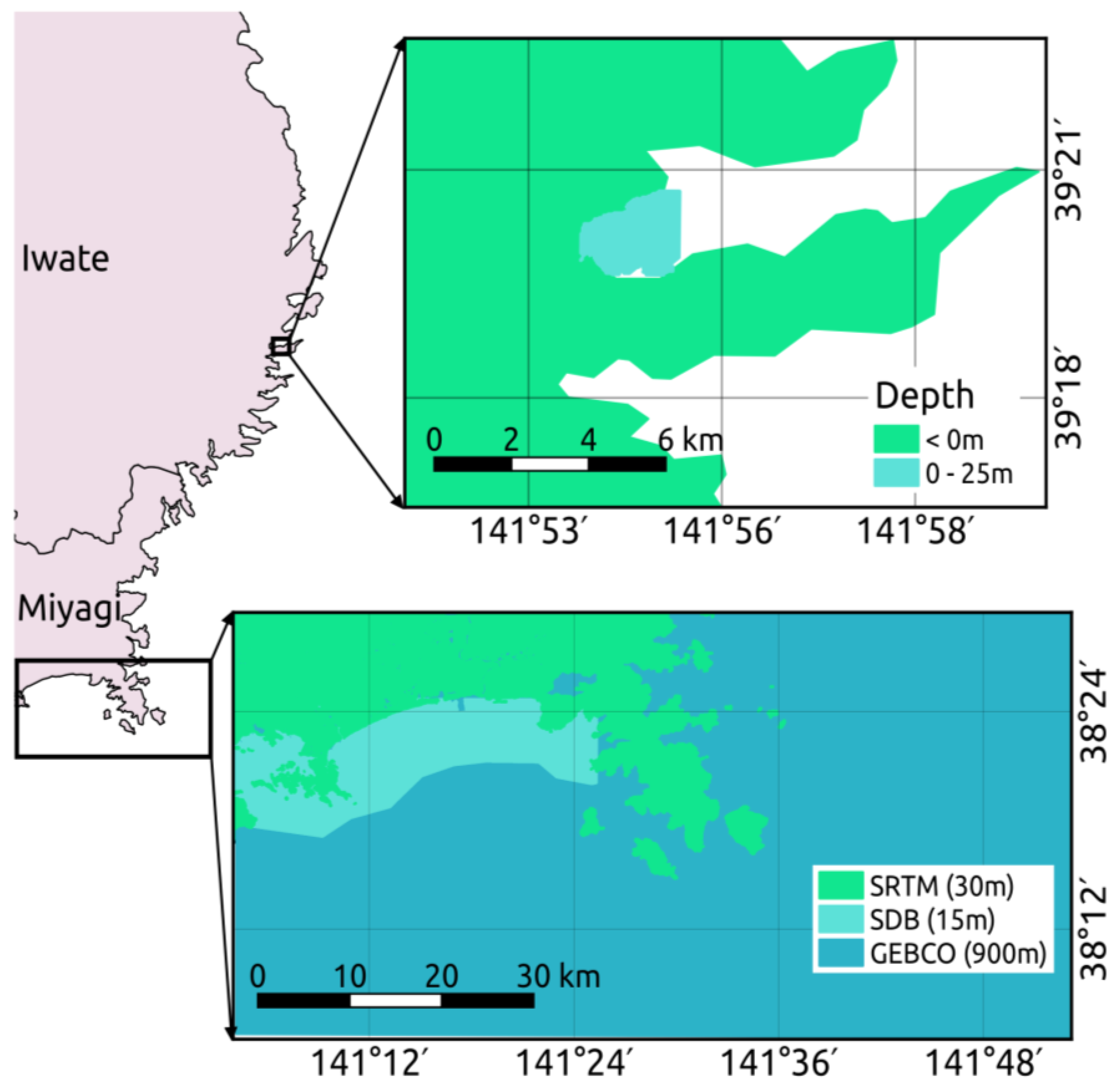
4.2. Iwate Prefecture, Japan

The second study demonstrates SDB estimation in a coastal area of the Iwate Prefecture, Japan (Figure 4). This study area is comparatively much smaller than the previous study area, covering only 4 km² and stretching along 6 km of coast line. Freely available Landsat-8 with medium spatial resolution (30 m) and high radiometric resolution was collected on 31 October 2014. Higher radiometric resolution quantized over a 12-bit dynamic range and rescaled to a 16-bit dynamic range was used for SDB estimation. All the available visible spectral bands and the NIR band were used for estimation and the SWIR band (1.57–1.65 μm) band was used for correction. A total of 3360 depth points (10 June 2012) were collected by an echo sounder, 2342 depth points were used for estimation, and the remaining depth points were used to evaluate the accuracy of the result. Both the calibration and validation depth points ranged from 0 to 26 m.

The tide height during the acquisition of satellite imagery was nearly 1.35 m and was provided as tide height value in the module option to apply correction. A global model was used to estimate SDB in order to compare the accuracy and investigate the significant improvements provided by GWR based models (Table 2). Various weighting functions in Fixed-GWR and A-GWR were tested. Among them, A-GWR using bi-square kernel produced high accuracy SDB in terms of R (0.98), R² (0.97), and RMSE (1.50 m). Detailed results of the SDB are shown in

Table 3. Performance of i.image.bathymetry in case studies 1, 2, and 3.

Area	Data	Kernel	GWR Model	Time (m)	SDB Results
					R	R2	RMSE (m)
Puerto Rico	Sentinel-2	Gaussian	Fixed-GWR	2.22	0.99	0.98	0.67
			A-GWR	180.00	0.99	0.98	0.62
		Bi-square	Fixed-GWR	2.24	0.99	0.98	0.64
			A-GWR	184.00	0.99	0.98	0.61
Iwate	Landsat-8	Gaussian	Fixed-GWR	2.50	0.86	0.74	2.91
			A-GWR	6.00	0.96	0.93	1.54
		Bi-square	Fixed-GWR	2.50	0.88	0.77	2.77
			A-GWR	5.55	0.97	0.94	1.50
Miyagi	ASTER	Gaussian	Fixed-GWR	3.02	0.91	0.83	1.93
			A-GWR	265.00	0.89	0.80	2.20
		Bi-square	Fixed-GWR	3.08	0.93	0.87	1.65
			A-GWR	255.00	0.91	0.84	1.95

.

5. Application for Integrated Coastal Relief Model and Tsunami Simulation

The previous section illustrated that the newly developed i.image.bathymetry is able to produce high quality SDB. The results indicate that the module can be used to estimate SDB from various conditions of coastal water, density of calibration depth points, and spatial and radiometric resolutions of the satellite data. Therefore, in this section, this study investigates the application of derived SDB as input in practical scenarios. Our study aims to generate an ICRM over parts of the Miyagi Prefecture by combining derived SDB with various resolutions of topographic and bathymetry data. The ICRM could be used to demonstrate a practical application scenario of the SDB in a tsunami simulation to hindcast the real event. Coarse accuracy coastal bathymetry data were used for many previous tsunami simulation application researches. Several studies have reported issues pertaining to tsunami simulation due to lack of reliable accuracy coastal bathymetry data [30]. Hence, research aims to develop better ICRM in parts of the Miyagi Prefecture, Japan.

5.1. Study Area and Data Usage

Coastal areas in the Miyagi Prefecture, Japan were significantly affected by an earthquake driven tsunami that occurred off Japan on 11 March 2011 [31,32]. This tsunami was the third mega earthquake generated a tsunami in this decade. In view of this, tsunami simulation combining SDB and other datasets has been carried out in parts of the Miyagi Prefecture (Figure 4) along a 110 km long coastal stretch.

Medium spatial resolution (15 m) ASTER Open Data collected on 10 September 2010 were used to estimate SDB. Medium radiometric resolutions (8-bit quantized) in the green band (0.52–0.60 μm) and the red band (0.63–0.69 μm) were used for estimation and the NIR band (0.76–0.86 μm) Nadir looking was used for correction (Table 1). J-EGG500 (Japan Oceanographic Data Center (JDOC)-Expert Grid data for Geographic-500m) bathymetry data of 500 m grid resolution were used as calibration depth points to estimate 15 m reliable SDB approximately over an area of 219 km² in a part of the Miyagi coastal area. A total of 649 evenly distributed calibration depth points were used for calibration and for the evaluation of accuracy. Even though the depth points were sparse, the distribution of the data was at equal intervals. Therefore, a Fixed-GWR model was used to estimate the SDB and was expected to perform better than an A-GWR model in this situation. The results of SDB generated from Fixed-GWR shows better agreement with reference depth in terms of R (0.93), R² (0.87), and RMSE (1.65 m) than the A-GWR model with R (0.91), R² (0.84), and RMSE (1.95 m). Both the Advanced Spaceborne Thermal Emission and Reflection (ASTER) satellite image and the J-EGG500 data were collected before the tsunami occurred; therefore the estimated SDB can be considered to be reliable.

5.2. Integrated Coastal Relief Model

ICRM provides a comprehensive view of regional coastal zones, integrating offshore bathymetry with land topography into a seamless representation of the coast. Here, ICRM was generated to provide a seamless representation of parts of the Miyagi Prefecture. This model incorporates the most recent publicly available topographic data and bathymetry data (Figure 4). Publicly available low resolution (900 m) offshore bathymetry collected from General Bathymetry Chart of the Oceans (GEBCO) and medium resolution (30 m) terrestrial topographic data collected from Shuttle Radar Topographic Mission (SRTM) [33] were combined with SDB estimated using ASTER (15 m) to develop the seamless ICRM. The ICRM was generated using an ANUGA Open Source Hydrodynamic model [34]. ANUGA is an Open Source Software package, with most components being implemented in Python, and is capable of modeling the impact of hydrological disasters such as dam breaks, riverine flooding, storm-surges, or tsunamis. ANUGA functions provide a platform to combine multiple spatial resolution raster data sets for a comprehensive ICRM.

Firstly, the raster GEBCO, SRTM, and SDB data were individually converted to American Standard Code for Information Interchange (ASCII) format with Universal Transverse Mercator (UTM) coordinates using the r.out.ascii module of GRASS GIS. Further this ASCII data was converted into Digital Elevation Model (DEM) format using the script anuga.asc2dem. Further, the DEM file was converted to point format using anuga.dem2pts. Subsequently the point file containing multi-resolution topographic data was combined using the ANUGA script anuga.geospatial_data.geospatial_data, and a single seamless ICRM was generated.

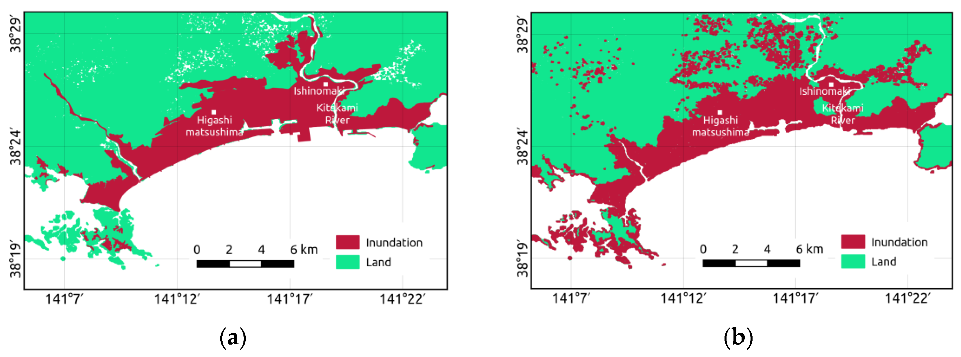
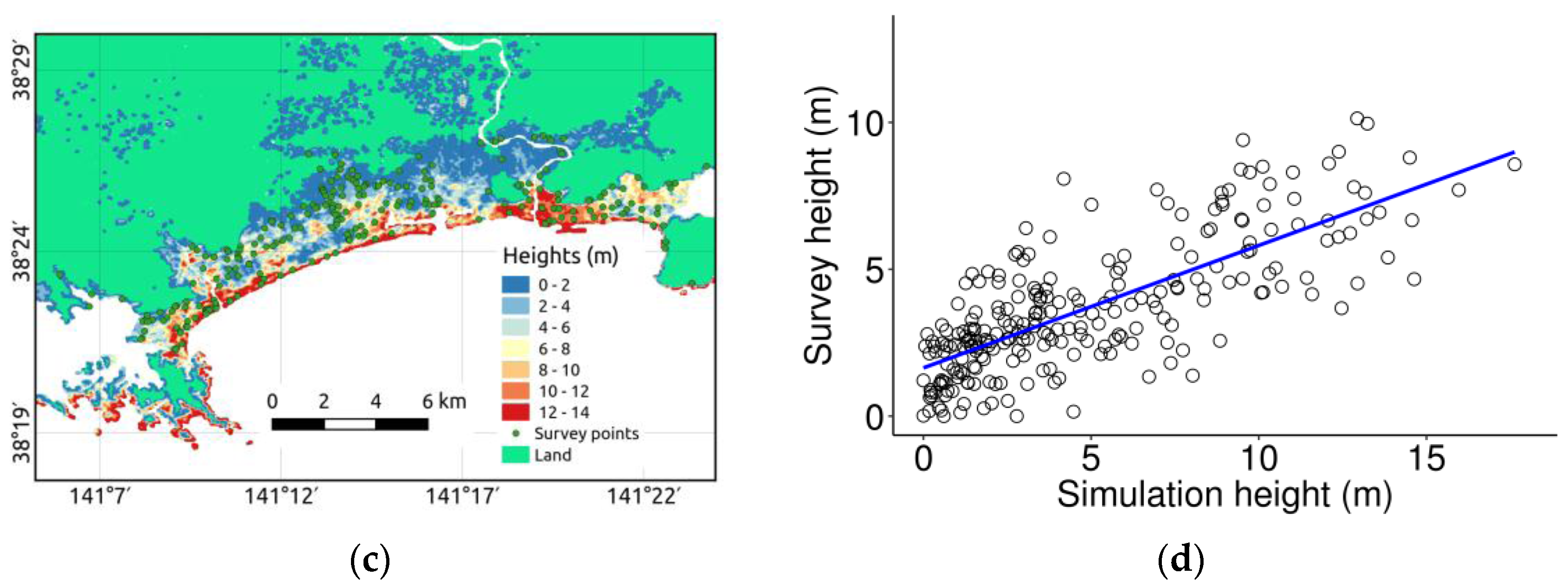
5.3. Tsunami Simulation

In the case of tsunami simulation, 2D non-linear shallow water equations are commonly implemented and solved numerically on a mesh or grid, and there are many software solutions available for tsunami simulation, such as TUNAMI [35], ANUGA, and TsunAWI [36]. Tsunami inundation is simulated through numerical solutions of the non-linear shallow water equations over a model of bathymetry and topography with appropriate extensions to model wetting and drying processes. ANUGA uses unstructured triangular meshes, with internal polygons used to define the maximum allowable size of an individual mesh. The ICRM represents unstructured triangular meshes, as explained in Section 5.2. The Tohoku tsunami was generated from the crust sliding after earthquake; therefore a crust slide generated tsunami simulation was carried out. The available python script runcairns.py in ANUGA was adopted and modified for our simulation experiment. Boundary conditions such as rainfall, tide, wind stress, surface roughness, etc. were not considered in the simulation process. In addition, mean sea level was assumed as the initial water level and a fixed manning’s coefficient was used.

6. Result and Discussion

This study presents a user friendly Open Source GIS module to estimate bathymetry from optical satellite imageries. The efficacy of the i.image.bathymetry module has been evaluated using three case studies with multi-resolution and multi-constellation data. The module incorporates pre-processing of satellite data and an option for performing tide correction of calibration depth data with tide at the time of satellite image capture. The SDB estimation region is automatically determined by the distribution of calibration depth points. Therefore it is suggested to be mindful while preparing the calibration depth points in order to cover the area of interest. In addition, an optional parameter has been developed to supply a polygon vector file which defines the area to be estimated. Deep water pixels are used for atmosphere and water corrections; therefore, users need to provide multispectral data, which contains deep water regions. A satellite image that does not have a deep water region can also be used for SDB estimation without applying deep water pixels for correction. If deep water regions are not supplied, the correction band will be used for correction without the use of deep water regression coefficients. In addition, our previous studies [20] have suggested the use of the SWIR band for correction instead of the NIR band. NIR band is suggested to be used for correction only when multispectral imagery does not include the SWIR band, such as imageries like ASTER. The key functionality of the i.image.bathymetry module is GWR based estimation. Our present and earlier research [20] have demonstrated that the GWR model can effectively address the issues of heterogeneity due to different bottom types and water quality and hence provide improved SDB.

A major limitation in SDB models is the inability to address the spatial heterogeneity due to different bottom types and water types. The presented module proposed to address this issue by using a GWR based model. The results shown in Table 2 and

Table 4. Statistical differences between reference depth and SDB in case studies 1, 2, and 3.

Case Studies	Reference Depth				GWR Model
	Min	Max	Mean	STD	Min	Max	Mean	STD
Puerto Rico	0.80	20.20	10.89	4.89	0.82	20.10	10.83	4.94
Iwate	0.48	26.51	11.95	5.89	0.53	26.29	11.99	6.00
Miyagi	2.00	19.00	11.95	4.90	1.51	17.41	12.10	3.45

clearly indicate the improvements made by the proposed module by addressing local heterogeneity issues. The statistical difference between reference depth and estimated SDB illustrated in Table 4 shows a good agreement with each other for all the three case studies.

The presented case studies were carried out in order to assess the behavior and performance of the module related to different factors such as size of the data, spatial/spectral/radiometric resolution, cloud coverage, and water quality of the study area. Table 3 evaluates the performance of the module in order to comprehend impact of above mentioned factors in SDB estimation. Table 3 mainly compares the accuracy of the results in terms of kernel weighting functions (bi-square or Gaussian) and the mode of the GWR estimation (Fixed-GWR or A-GWR). The machine used for the benchmark was a laptop with an Intel Core i5-3320M CPU @2.60 GHz. The system has 16 Gb of RAM and a solid-state disk (SSD) of 512 Gb. The installed operating system (OS) is GNU/Linux (Ubuntu 14.04 LTS x64-bit). GRASS 7.0.4 version and R version 3.3.1 were used for the benchmark. The screenshots shown in Figure 5 demonstrate the options and workflow of i.image.bathymetry. Figure 5 shows an example of case study 1 to demonstrate the processing using the bi-square kernel. Figure 5a shows the required input used in the processing and Figure 5b demonstrates the optional input and optional flags used for Fixed-GWR based SDB estimation. The -f flag used in Figure 5b can be removed in order to process A-GWR based SDB estimation. Figure 5c demonstrates the optimal bandwidth estimation procedure for Fixed-GWR based computation. The optimal bandwidth estimation begins from a minimum value. The module performs GWR computation once the optimal bandwidth is determined. In Figure 5c, 47 was determined as the optimal bandwidth for Fixed-GWR estimation. Figure 5d shows the A-GWR optimal bandwidth estimation in R using a cross-validation score. The number of points (15) selected as the optimal adaptive bandwidth is shown in Figure 5d. Figure 5e,f show the SDB estimated using Fixed-GWR and A-GWR in the GRASS GIS monitor, respectively.

The area covered (40 km²) in case study 1 (Figure 1) was relatively larger and the spatial/spectral/radiometric resolutions of the imagery used was higher than in case studies 2 and 3. Apart from that, there were more depth points used for calibration, and the water quality of the area was also relatively better. Therefore, case study 1 produced high accuracy SDB from both Fixed and A-GWR models (Table 3). The processing time was evaluated using Fixed-GWR and A-GWR with bi-square and Gaussian kernels. In the case of the Fixed-GWR model, around 2 min were needed to finish processing, and in the case of the A-GWR model, around 6 min were needed to finish the processing. Since the region used to estimate SDB was a continuous surface, it is obvious that both Fixed and A-GWR perform well [20]. In case study 1, the study area was a continuous surface with dense calibration points distributed randomly over relatively clear waters, thereby facilitating SDB generation with good accuracy SDB for both the Fixed and A-GWR models.

The second study area covered (4 km²) a part of the Iwate Prefecture (Figure 2) and was relatively smaller than the area in case study 1, and SDB estimation was based on a medium spatial resolution of 30 m. In the case of the Fixed-GWR model, around 2.5 min were needed to finish processing, and in case of A-GWR model, around 180 min were needed to finish the processing (Table 3). A-GWR with a bi-square kernel provides a better SDB estimate compared to the other modes. In case study 2, a continuous surface of the study area and randomly distributed denser calibration depth points were considered as two favorable factors for better estimation using the A-GWR model. The Fixed-GWR model does not perform well in this area, which could perhaps be the result of low quality water in study area.

Figure 4 shows the third study area with the parts of the Miyagi Prefecture that were used for ICRM generation and tsunami simulation. In the case of the Fixed-GWR model, around 3 min were taken to finish processing. In case of A-GWR model, around 260 min were taken to finish the processing (Table 3). The calibration depth points were sparse and distributed in unit intervals (500 m), and, hence, the Fixed-GWR model was expected to provide better or almost similar estimates to the A-GWR model [26]. Fixed-GWR with a bi-square kernel provides better SDB.

The above case studies elucidate the efficacy of the i.image.bathymetry in estimating SDB and provide useful input for ICRM in tsunami simulation. Tsunami simulation was carried out with duration of 50 min and results were evaluated with post-tsunami survey results [33]. The main earthquake shocks lasted for 3 to 4 min, and, owing to the proximity of the epicenter to shore, the first significant waves reached Japan only 10 min after the event started [37]. In this study, we compared the inundation extent and heights of the tsunami simulation with post-tsunami survey data. The simulation experiment shows that an area of around 115 km² was inundated. The simulation tsunami about 14 m high traveled inland up to 5 kilometers, and the Ishinomaki and Higashimatsushima regions were affected the most. These regions are low lying land, and Kitakami River passes through the Ishinomaki region; these factors could have contributed to amplifying the tsunami inundation (Figure 6).

Figure 5 illustrates the comparison between the simulation results and the post-tsunami survey results. Figure 6a shows the actual extent of the inundation, and Figure 6b shows the simulated inundation extent over 50 min. The surveyed tsunami inundation heights at 243 points were overlaid on a simulated tsunami inundation height map (Figure 6c). Figure 6d demonstrates the correlation between the surveyed and simulated tsunami inundation heights. Figure 6c,d show that the maximum inundation observed was about 10 m and 14 m in surveyed and simulated events, respectively. The evaluation of the simulated tsunami inundation heights shows a reasonable agreement with post-tsunami survey data in terms of R (0.75), R² (0.57), and RMSE (2.98 m).

7. Conclusions

Our study concludes that the i.image.bathymetry GRASS GIS module can be considered an effective solution for SDB. The module can be downloaded from https://svn.osgeo.org/grass/grass-addons/grass72/imagery/ or installed using the g.extension module in GRASS GIS. The accuracy of SDB depends upon characteristics of satellite imagery, number and distribution of calibration depth points, and water conditions of the study area. All the case studies were aimed to evaluate the performance of the module in addressing the characteristics of the data, which varied depending on the data used and area investigated. The i.image.bathymetry module allows the user to choose both a Fixed and an A-GWR model with either a bi-square or Gaussian kernel weighting function; this option can be effectively used if the user has prior knowledge about the study area. This study also evaluated the computational cost for estimation of Fixed and A-GWR models, comparing the accuracy of the SDB generated. Such evaluation illustrates that an A-GWR model is computationally intensive, especially for a large dataset, but offers the best results. However both Fixed and A-GWR models estimated SDB with acceptable accuracy, and, hence, it is suggested to use either Fixed or A-GWR according to the distribution of calibration depth points, size of the image, and available RAM on the computer.

A common problem in SDB is the tide differences between the calibration depth and the satellite image; therefore the module allows the tide correction to be carried out if the tide height during the acquisition of satellite imagery was provided. A radiative transfer model is inherently related to the penetration capacity of light to the bottom of the sea and provides information about water depth. However, better accuracy can be expected in clear waters even with the minimum number of calibration depth points. The i.image.bathymetry module effectively addresses the problem of heterogeneity in bottom types and water quality using multispectral bands in a GWR model. Our results indicate that all the available spectral bands in the visible spectral domain can be provided to the module for better SDB estimation.

This study has demonstrated application examples of SDB in a tsunami simulation model. The results of the tsunami simulation show reasonably good agreement with post-tsunami survey results. The future perspective for the study is to deploy i.image.bathymetry as a Web Processing Service (WPS) to facilitate on-demand SDB data to the user without requiring them to have software and data locally. In case of Japan, low resolution (500 m) depth data (J-EGG500) are available as Open Data. J-EGG500 depth data coupled with Open satellite images like Landsat-8, ASTER, Sentinel-2, etc. could be used with SDB as a service to users with limited expertise in Remote Sensing and geospatial analysis. GRASS GIS also offers a framework for parallel computing, which may be useful when considering the future implementation of the SDB algorithm as a Web Service.

References

1. Lyzenga, D.R. Remote sensing of bottom reflectance and water attenuation parameters in shallow water using aircraft and Landsat data. Int. J. Remote Sens. 1981, 2, 72–82. [Google Scholar] [CrossRef]
2. Baban, S.M.J. The evaluation of different algorithms for bathymetric charting of lakes using Landsat imagery. Int. J. Remote Sens. 1993, 14, 2263–2273. [Google Scholar] [CrossRef]
3. Benny, A.H.; Dawson, G.J. Satellite imagery as an aid to bathymetric charting in the Red Sea. Cartogr. J. 1983, 20, 5–16. [Google Scholar] [CrossRef]
4. Muslim, A.M.; Foody, G.M. DEM and bathymetry estimation for mapping a tide-coordinated shoreline from fine spatial resolution satellite sensor imagery. Int. J. Remote Sens. 2008, 29, 4515–4536. [Google Scholar] [CrossRef]
5. Philpot, W.D. Bathymetric mapping with passive multispectral imagery. Appl. Opt. 1989, 28, 1569–1579. [Google Scholar] [CrossRef] [PubMed]
6. Stumpf, R.P.; Holderied, K.; Sinclair, M. Determination of water depth with high-resolution satellite imagery over variable bottom types. Limnol. Oceanogr. 2003, 48, 547–556. [Google Scholar] [CrossRef]
7. Clark, R.K.; Faye, T.H.; Walker, C.L. Bathymetry using thematic mapper imagery. Ocean Opt. IX 1988, 925, 229–231. [Google Scholar]
8. Stoffle, R.W.; Halmo, D.B. Satellite Monitoring of Coastal Marine Ecosystems: A Case from the Dominican Republic; Consortium for Integrated Earth Science Information Network (CIESIN): Saginaw, Michigan, 1991. [Google Scholar]
9. Lyzenga, D.R.; Malinas, N.R.; Tanis, F.J. Multispectral bathymetry using a simple physically based algorithm. IEEE Trans. Geosci. Remote Sens. 2006, 44, 2251–2259. [Google Scholar] [CrossRef]
10. Gholamalifard, M.; Esmaili Sari, A.; Abkar, A.; Naimi, B. Bathymetric modeling from satellite imagery via single band algorithm (SBA) and principal components analysis (PCA) in southern Caspian Sea. Int. J. Environ. Res. 2013, 7, 877–886. [Google Scholar]
11. Vinayaraj, P.; Raghavan, V.; Masumoto, S.; Glejin, J. Comparative evaluation and refinement of algorithm for water depth estimation using medium resolution remote sensing data. Int. J. Geoinform. 2015, 11, 17–29. [Google Scholar]
12. Kanno, A.; Tanaka, Y. Modified lyzenga’s method for estimating generalized coefficients of satellite-based predictor of shallow water depth. IEEE Geosci. Remote Sens. Lett. 2012, 9, 715–719. [Google Scholar] [CrossRef]
13. Monteys, X.; Harris, P.; Caloca, S.; Cahalane, C. Spatial prediction of coastal bathymetry based on multispectral satellite imagery and multibeam data. Remote Sens. 2015, 7, 13782–13806. [Google Scholar] [CrossRef]
14. Brunsdon, A.C.; Fotheringham, S.; Charlton, E.M. Geographically weighted regression: A method for exploring spatial nonstationarity. Geogr. Anal. 1996, 28, 283–297. [Google Scholar] [CrossRef]
15. Fotheringham, A.S.; Charlton, M.E.; Brunsdon, C. Geographically weighted regression: A natural evolution of the expansion method for spatial data analysis. Environ. Plann. 1998, 30, 1905–1927. [Google Scholar] [CrossRef]
16. Lu, B.; Harris, P.; Charlton, M.; Brunsdon, C. The GWmodel R package: Further topics for exploring spatial heterogeneity using geographically weighted models. Geo-Spat. Inf. Sci. 2014, 17, 85–101. [Google Scholar] [CrossRef]
17. Chen, G.; Zhao, K.; Mcdermid, G.J.; Hay, G.J. The influence of sampling density on geographically weighted regression: A case study using forest canopy height and optical data. Int. J. Remote Sens. 2012, 33, 2909–2924. [Google Scholar] [CrossRef]
18. Yrigoyen, C.C.; Rodrigouz, I.G.; Otera, J.V. Modeling spatial variations in household disposable income with geographically weighted regression. Estad. Esp. 2008, 50, 321–360. [Google Scholar]
19. Su, H.; Liu, H.; Lei, W.; Philipi, M.; Heyman, W.; Beck, A. Geographically adaptive inversion model for improving bathymetric retrieval from multispectral satellite imagery. IEEE Trans. Geosci. Remote Sens. 2013, 52, 465–476. [Google Scholar] [CrossRef]
20. Vinayaraj, P.; Raghavan, V.; Masumoto, S. Satellite derived bathymetry using adaptive-geographically weighted regression model. Mar. Geod. 2016, 39, 458–478. [Google Scholar] [CrossRef]
21. Neteler, M.; Bowman, H.; Landa, M.; Metz, M. GRASS GIS: A multi-purpose open source GIS. Environ. Model. Softw. 2012, 31, 124–130. [Google Scholar] [CrossRef]
22. Python Software Foundation. 2016. Available online: https://www.python.org/ (accessed on 07 January 2017).
23. Zambelli, P.; Gebbert, S.; Ciolli, M. Pygrass: An object oriented Python Application Programming Interface (API) for Geographic Resources Analysis Support System (GRASS) Geographic Information System (GIS). ISPRS Int. J. Geo-Inf. 2013, 2, 201–219. [Google Scholar] [CrossRef]
24. R Core Team. R: A Language and Environment for Statistical Computing; R Foundation for Statistical Computing: Vienna, Austria, 2016. [Google Scholar]
25. Bivand, R. Interface between GRASS 7 Geographical Information System and R 2015. Available online: https://cran.r-project.org/web/packages/rgrass7/ (accessed on 07 January 2017).
26. Gollini, I.; Lu, B.; Charlton, M.; Brunsdon, C.; Harris, P. GWmodel: An R Package for exploring spatial heterogeneity using geographically weighted models. J. Stat. Softw. 2015, 63, 1548–7660. [Google Scholar] [CrossRef]
27. Harris, P.; Fotheringham, A.S.; Crespo, R.; Charlton, M. The use of geographically weighted regression for spatial prediction: an evaluation of models using simulated data Sets. Math. Geosci. 2010, 42, 657–680. [Google Scholar] [CrossRef]
28. Harris, P.; Brunsdon, C.; Fotheringham, A.S. Links, comparisons and extensions of the geographically weighted regression model when used as a spatial predictor. Stoch. Environ. Res. Risk Assess. 2011, 25, 123–138. [Google Scholar] [CrossRef]
29. Costa, B.M.; Battista, T.A.; Pittman, S.J. Comparative evaluation of airborne lidar and ship-based multibeam sonar bathymetry and intensity for mapping coral reef ecosystems. Remote Sens. Environ. 2009, 113, 1082–1100. [Google Scholar] [CrossRef]
30. Griffin, J.D.; Latief, H.; Kongko, W.; Harig, S.; Horspool, N.; Hanung, R.; Rojali, A. An evaluation of onshore digital elevation models for modeling tsunami inundation zones. Front. Earth Sci. 2015, 3, 1–16. [Google Scholar] [CrossRef] [Green Version]
31. Akio, O.; Takenori, S.; Hidekatsu, Y.; Takeyoshi, N.; Shinji, S. Severe erosion of sandbar at Unosumai River mouth, Iwate, due to 2011 Tohoku tsunami. In Proceedings of the 7th International Conference on Coastal Dynamics, Arcachon, France, 24–28 June 2013.
32. Mori, N.; Takahashi, T. Nationwide post event survey and analysis of the 2011 Tohoku earthquake tsunami. Coast. Eng. J. 2012, 54, 1250001. [Google Scholar] [CrossRef]
33. Shuttle Radar Topography Mission1 Arc-Second Global. 2015. Available online: https://lta.cr.usgs.gov/SRTM1Arc (accessed on 07 January 2017).
34. Nielsen, O.; Roberts, S.; Gray, D.; McPherson, A.; Hitchman, A. Hydrodynamic modeling of coastal inundation. In MSSANZ International Congress on Modelling and Simulation; Modelling and Simulation Society of Australia and New Zealand: Melbourne, VIC, Australia, 2005; pp. 518–523. [Google Scholar]
35. Goto, C.; Ogawa, Y.; Shuto, N.; Imamura, F. IUGG/IOC Time Project: Numerical Method of Tsunami Simulation with the Leap-Frog Scheme; IOC Manuals and Guides No. 35; IOC of UNESCO Publish: Paris, France, 1997. [Google Scholar]
36. Rakowsky, N.; Androsov, A.; Fuchs, A.; Harig, S.; Immerz, A.; Danilov, S. Operational tsunami modelling with TsunAWI—recent developments and applications. Nat. Hazards Earth Syst. Sci. 2013, 13, 1629–1642. [Google Scholar] [CrossRef] [Green Version]
37. Grilli, S.T.; Harris, J.C.; Tajalli Bakhsh, T.S.; Masterlark, T.L. Numerical simulation of the 2011 Tohoku tsunami based on a new transient FEM co-seismic source: Comparison to far and near-field observations. Appl. Geophys. 2013, 170, 1333–1359. [Google Scholar] [CrossRef]
Figure 1. Flowchart of the workflow of i.image.bathymetry.
Ijgi 06 00089 g001
Figure 2. Case study 1: Study area, Puerto Rico, Northeastern Caribbean Sea.
Ijgi 06 00089 g002
Figure 3. Comparison between residual maps of (a) global model and (b) Geographically Weighted Regression (GWR) model for case study 1.
Ijgi 06 00089 g003
Figure 4. Case study 2 and 3: Study area, parts of the Iwate Prefecture and the Miyagi Prefecture, Japan.
Ijgi 06 00089 g004
Figure 5. These screenshots demonstrate the input options and processing of i.image.bathymetry using an example from case study 1, (a) required input bands; (b) optional input bands and optional flags selected for Fixed-GWR; (c) optimal bandwidth estimation for Fixed-GWR; (d) optimal bandwidth estimation for A-GWR; and (e) SDB estimated from Fixed-GWR and (f) SDB estimated from A-GWR.
Ijgi 06 00089 g005
Figure 6. Evaluation of Tohoku tsunami simulation results with post survey data. (a) Actual tsunami inundation extent; (b) simulation inundation extent; (c) survey tsunami height points overlaid on simulated tsunami inundation height map; and (d) scatter plot between survey and simulation tsunami height points.
Ijgi 06 00089 g006aIjgi 06 00089 g006b