
Analysis of Burglary Hot Spots and Near-Repeat Victimization in a Large Chinese City


1
College of Civil Engineering, Nanjing Forestry University, Nanjing 210037, China
2
Key Laboratory of Virtual Geographic Environment, Ministry of Education, Nanjing Normal University, Nanjing 210046, China
3
Jiangsu Center for collaborative Innovation in Geographical Information Resource Development and Application, Nanjing 210023, China
4
Key Laboratory of Police Geographic Information Technology, Ministry of Public Security, Nanjing 210046, China
*
Author to whom correspondence should be addressed.
ISPRS Int. J. Geo-Inf. 2017, 6(5), 148; https://0-doi-org.brum.beds.ac.uk/10.3390/ijgi6050148
Submission received: 17 March 2017
/
Revised: 5 May 2017
/
Accepted: 8 May 2017
/
Published: 10 May 2017
Abstract
:A hot spot refers to numerous crime incidents clustered in a limited space-time range. The near-repeat phenomenon suggests that every victimization might form a contagion-like pattern nearby in terms of both space and time. In this article, the near-repeat phenomenon is used to analyze the risk levels around hot spots. Utilizing a recent burglary dataset in N (a large city located in southeastern China), we examine the near-repeat phenomenon, the results of which we then use to test the contributions of hot spots. More importantly, we propose a temporal expanded near-repeat matrix to quantify the undulation of risk both before and after hot spots. The experimental results demonstrate that hot spots always form. Space-time areas of high risk are always variable in space and time. Regions in the vicinity of hot spots simultaneously share this higher risk. In general, crime risks around hot spots present as a wave diffusion process. The conclusions herein provide a detailed analysis of criminal patterns, which not only advances previous results but also provides valuable research results for crime prediction and prevention.
1. Introduction
The spatial distribution of crime varies temporally. To interpret this changing process, researchers have attempted to analyze crime patterns and have observed the existence of interactions called the repeat and near-repeat phenomena among burglaries [1]. These phenomena indicate that, shortly following a burglary, locations within the immediate proximity are more susceptible to experiencing the same event. The rhythm, characterizing crime, provides critical information about criminal activity. More recently, space-time patterns have also been observed among different crime types such as residential burglaries [2], street robberies [3], and gun violence [4]. However, few studies have considered the space-time pattern around hot spots. Utilizing a set of burglary data from N, a city located in southeast China, this paper attempts to investigate whether a near-repeat phenomenon exists in N city. The relationship between near-repeat victimization and hot spots will also be investigated. Furthermore, to analyze the displacement process of hot spots, we expand the near-repeat matrix to investigate the relationship between hot spots and near-repeat phenomena.
2. Theoretical Background
2.1. Environmental Criminology
Since the 20th century, coordinates of crimes have been marked on a map by researchers [5]. Numerous studies have shown that crime incidents are spatially concentrated [6]. Hot spots are proposed and defined as locations with a larger concentration of crime than is average [7]. There are several theories that have been proposed to explain why those areas are more likely to attract criminals, such as routine activities, rational choice, and crime pattern theory [8,9]. Cohen and Felson’s [8] routine activity theory provides an explanation of crime problems in that a motivated offender, an attractive target, and the absence of a controller are three indispensable factors in the occurrence of crime. A crime will not occur if any of the three elements is absent. Using this theory, many crimes may become concentrated within certain areas because of people’s highly repetitive daily routines. Clarke’s [9] rational choice theory adopts a utilitarian belief that man reasons based on weighing both means and ends and both costs and benefits, subsequently making a rational choice. Every crime incident is a purposeful behavior following consideration of various types of information to satisfy the offender’s needs. The crime pattern theory assumes crime locations to be a registered residence by an offender [10,11]. An attractive node has a greater probability of being given attention by offenders. As a result, crimes occur unevenly in time and space. Generally, all criminal theories argue that a vulnerable environment may be characterized by the possibility for crime to occur. A vulnerable target (or place) may attract more offenders and lead to a concentration of criminal activity.
2.2. Repeat and Near-Repeat Victimization
Some researchers have worked to integrate the interaction components of space and time. Researchers have found that offenders are more likely to repeat another crime at the same location rather than move to a new location [12]. This phenomenon is called repeat victimization. Other researchers have found phenomena of increasing risk among areas near the location, which is called near-repeat victimization [13]. Numerous studies have investigated the existence of repeat and near-repeat victimization for various crime types [2,3,4]. Two accounts have been presented to interpret the mechanism of repeat and near-repeat victimization; the boost and flag accounts. Boost theory suggests that the heightened risk of future victimization is boosted by past victimization [12,14,15,16]. In this theory, it is assumed that previous offenders communicate information about objects (or locations) to future offenders. Future offenders gain information about a target and return to the area of a previous offence for future victimizations. Flag theory argues that certain target properties may be flagged by opportunistic offenders. Thus, future victimizations will become concentrated because of the attractiveness of targets independent of the offender. Both the boost and flag accounts have been tested and used in many studies [17,18,19].
Quantitative research concerning repeat and near-repeat victimization has also been conducted by many researchers. Some investigations have used the Knox method to quantify the risk level after every crime event [20]. Townsley and colleagues investigated burglary data for Queensland, Australia, and concluded that an area within 200 m over a time span of two months exhibits a higher risk level for criminal activity [21]. Research in Merseyside, UK, found a higher risk area of 400 m and a time span of 2 months [1]. The repeat and near-repeat patterns were found to have different areas in many studies [22,23]. This problem may be caused by the differences between research areas. More recently, mathematicians have used statistical methods to quantify the influence of crime events [24]. The conclusion of quantitative research has been that both repeat and near-repeat patterns are critically important for crime prediction [25,26].
2.3. Hot Spot and Near-Repeat Victimization
Recent studies on hot spots have started to focus on spatial and spatial-temporal dimensions [27,28,29,30]. To interpret the mechanism underlying the formation of hot spots, the relationship between hot spots and near-repeat victimization has also attracted the attention of scholars. Haberman and Ratcliffe investigated how near-repeat victimizations contribute to the development and subsequent temporal stability of crime hot spots [31]. In this study, some temporally stable hot spots contain a great number of near-repeat events. Other researchers have tested the involvement of the same offender in near-repeat burglaries [32]. The experimental results show that same-offender involvement is very high for near-repeat victimizations. Thus, events in hot spots may also be committed by the same offender. These conclusions are chiefly focused on how the ‘gathering’ characteristic leads to a ‘gathering’ phenomenon regarding victimizations [33]. However, the infinite aggregation of crime cannot continue, and it is difficult to simply use ‘near-repeat’ victimization to explain the dynamic activities involved with crime hot spots.
An alternative hypothesis about the dynamic characteristics of crime is the spatial and temporal displacement characteristic of crime hot spots. The displacement phenomenon can be described as follows: when the crime level in one cluster increases, the crime level in another cluster region decreases and vice-versa [33]. Brunsdon intuitively presented the variable mechanisms of crime hot spots in a space-time cube after using a kernel density estimation [29]. The spatial and temporal displacements of hot spots could be clearly shown through visualization techniques. To verify the displacement of crime, geographers have also displayed hot spots on road networks. The experimental results concluded that crime hot spots are displaced temporally [23]. Alternatively, data mining methods are also used to analyze the temporal patterns of crime displacement [34]. Piquero interpreted the displacement of hot spots as resulting from the rational choices of crime offenders interacting with local policing activities [35]. Robinson’s explanation for hot spot displacement is considered to be more classical in that offenders vary their activities to avoid local police and that informal crime-prevention activities, which are often intensified after a sharp increase in criminal activity, initiate in a local area [36]. This relationship between crime displacement and location patrol mode has been tested by Groff and Johnson. After an analysis of walking and vehicle patrols, Groff discovered that each patrol mode has a decreasing effect on the crime level [37]. These studies analyzed crime patterns from a different perspective and thus expanded the research on criminology.
In summary, current studies focus on the ‘gathering’ of crime incidents and the ‘displacement’ of hot spots, leading to many conclusions regarding crime patterns. However, it is also important to analyze what occurred around hot spots from a quantitative point of view. Understanding when and where crime incidents occur and cluster or displace can alternatively advance theoretical explanations of crime patterns. Different crime patterns tend to generate different prevention strategies. A study of relevant mechanisms is important for criminal investigations and can help optimize police patrols more efficiently toward decreasing crime levels. Based on a theoretical and analytical framework derived from previous research, our analysis consists of three parts. First, we utilize recorded burglary data to assess if near-repeat phenomena exist in the research area. Second, we select burglaries within hot spots to investigate the level of hot spot involvement in detected burglary pairs based on their spatial and temporal closeness. Based on the experimental results, we examine the potential relationships among hot spots and near-repeat phenomena. Third, we expand the time axis of the Knox matrix to analyze the displacement of hot spots. More specifically, we examine the characteristics of hot spot precursors and the nature of events that occur following the formation of a hot spot. We then conclude by summarizing our findings and by discussing the practical implications and limitations of this study.
3. Materials
3.1. Study Area
The study area (31°14´ E–32°37´ E, 118°22´ N–119°14´ N) is located in the economically developed Yangtze River Delta region, covering a total area of 263.43 km2 (Figure 1). Being the capital of Jiangsu province, N city is a core transportation hub, from which one is capable of reaching every city within the Yangtze River Delta region within 1 h. N consists of four boroughs; Gulou, Xuanwu, Qinhuai, and Jianye. The downtown area has retained a large number of ancient buildings. The suburbs are an economic development zone and possess a large number of new buildings. The region has a continental climate, with a mean annual temperature of 15.6 °C and an annual precipitation of 534–1825.8 mm. Geographical advantages have allowed N city’s economy to achieve rapid development; thus, N is representative of China. Being a large city on the Yangtze River economic zone of China, N city offers an important contrast to evidence derived from earlier studies conducted in other cities of China and elsewhere in the world [38,39].
3.2. Data Sources
The research data used herein are burglary data acquired from an official crime dataset recorded through grassroots police efforts and are registered on the map. The full dataset includes a total of 4226 burglaries recorded from 1st January 2013 to 30th December 2013. Each record of the data includes the data and the location (XY coordinates) of the burglary. All of the dataset will be utilized to calculate the near-repeat matrix and analyze the displacement of the hot spots.
It should be noted that the local police department uses special geocoding for the locations of crime events. Only a few crime events have the same coordinate, leading to a small number of repeat victimizations. Current research on repeat and near-repeat victimizations classifies the repeat pairs as near-repeat pairs separated by a short spatial distance [40,41]. This method will also be used in this research.
4. Methods
4.1. Near-Repeat Matrix
The near-repeat matrix is calculated using the Knox method [1], which was originally developed to identify space-time clustering in epidemiology. The Knox method was also widely employed by criminology researchers after criminal activity was found to have the same spatial-temporal patterns as in epidemiology. The first step of the Knox method is to measure the spatial and temporal distances between each event and every other event within the dataset. Next, a spatial and temporal bandwidth will be specified to construct a matrix. The horizontal axis and the vertical axis represent the temporal and spatial distances, respectively. The resolution of every unit in the matrix depends on the temporal and spatial bandwidths. Thus, a one-point pair with an appropriate spatial and temporal distance will be filled into the compatible element. The value of a cell represents the number of point pairs filled into the cell. A Monte Carlo simulation is then used to create an expected distribution of cell values to determine if the cell values are greater than would be expected with sufficient probability. Each iteration of the Monte Carlo simulation returns a randomly distributed cluster of points in the same number as in the dataset. Then, another matrix is calculated using the Knox method. The near-repeat matrix is then calculated, unit by unit, using the matrix of the dataset divided by the expectation matrix generated by the Monte Carlo simulation. The confidence level of every unit will be determined by the number of observed units exceeding the expected unit values for all simulations. In the near-repeat matrix, values greater than 1 indicate a greater risk of criminal activity than expected, and values lower than 1 indicate a lower risk of criminal activity than expected.
Essentially, the near-repeat matrix is a risk model starting from every point in the dataset. The near-repeat matrix will indicate if there will be higher or lower risks of occurrence in the vicinity of another offence. According to existing research, a near-repeat matrix will present larger values in the top left of the matrix, resulting from the near-repeat phenomenon, which indicates a higher risk in the space-time proximity of a given crime event. This leads to the following question: what will occur after a crime hot spot forms?
A hot spot is represented by a space-time cell containing more crimes than expected. Most researchers focus on the risk after a single crime incident; few researchers investigate the risk around a crime hot spot. In this research, we will situate hot spots in the top left of the near-repeat matrix to indicate the risk level after one hot spot with other cells in the matrix. More significantly, to investigate the risk level prior to a hot spot, we expand the temporal axis to record the history before the occurrence of a given hot spot (Figure 2).
There have been several methods used to detect crime hot spots, including local autocorrelation methods [42], kernel density estimation [43], and Spatial and Temporal Analysis of Crime (STAC) [44,45]. STAC is widely used as a crime analysis tool in CrimeStat, inside which the search window is swept over the research area to determine if a sub-area can be classified into a hot spot based on the number of crime events within the sub-area. There are many types of shapes that can be defined as a search window [46,47]. In this research, a quadrate search window with cells of equal size in the near-repeat matrix is used to establish the matrix.
4.2. Temporal Expanded Near-Repeat Matrix
A temporal expanded near-repeat matrix (TENRM) is a matrix that records crime incident counts prior to and following each crime hot spot. The process for the calculation of a TENRM can be divided into two stages. The first stage is to uncover all the crime incidents within the hot spots. The second stage consists of risk testing based on the TENRM, similar to that of a near-repeat matrix.
The first stage will be divided into two steps. The first phase is to specify a space-time bandwidth , which will be used in the detection of hot spots and the resolution setting of the TENRM. In this research, the basic spatial and temporal bandwidths are 100 m and seven days, respectively. In the second step, the crime incidents within hot spots are detected through a statistical procedure [48]. Shiode defines crime hotspots as ‘a finite area with a significant level of elevated crime incident counts that are detected through a statistical procedure’. In this study, we use the same definition assumed by Shiode [48]. The space-time search windows will be generated using every data point as the center of the space and the starter at that time. A null model will be used to detect hotspots based on the assumption that crime incidents follow a Poisson distribution. Therefore, the probability of finding x number of crime incidents within the space-time bandwidth can be calculated as:
where is the expected number of crime incidents within A. Under the null hypothesis that is an independent Poisson random variable with the expected value of , the cumulative probability of having at least number of crime incidents observed in is:
If the cumulative probability calculated for the observed incidents within is less than the significance level , then the null hypothesis is rejected and these incidents are considered to form a hot spot. Two spatially or temporally adjacent hot spots can merge into one hotspot.
The second stage is composed of the remaining three steps. The third step in the overall algorithm is to construct a temporal expanded matrix that is twice the temporal size of the near-repeat matrix. In the temporal expanded matrix, the vertical axis and horizontal axes represent the spatial and temporal distances, respectively. The fourth step is to establish the number of space-time distances between hot spots and other points in the relevant elements of the TENRM. The earliest point to the other points will be used to represent the distance between the hot spot and other points. Thus, all hot spots will be located at the top center of the TENRM. The last step is a risk test based on a Monte Carlo simulation. Each count in the TENRM will be compared against all expected values, which are generated through 999 permutations, to the risk level of each corresponding space-time band [4]. For instance, when the observed number of incident pairs in a specific space-time band is greater than 996 for the simulated values, the significance level is 1–996/(9991) = 0.004. The risk level within a specific space-time band is the ratio of the observed number of incidents and the average number from the simulations. A larger ratio means a higher risk level in the space-time band.
5. Case Studies
5.1. Near-Repeat Characteristics of Research Area
The near-repeat matrix illustrates the risk level following a crime incident. In the top-left cell of Table 1, the value of 2.85 indicates that, once a crime incident occurs, another crime incident may transpire within 100 m during the next seven days, as the risk level increases by up to 175% over the normal level. Within the range of 100 m, all the cells within a 42 day period exhibit a higher risk level. This means that the risk level after a crime incident will be heightened for approximately six weeks. From the table, we can see that the top-left cell value is the largest and that the other cell values gradually decrease. Within 14 days and 300 m, the Knox ratios are significantly higher than 1.5. In summary, the experimental results demonstrate an obvious near-repeat phenomenon for burglaries in N.
According to the latest research, burglaries in Beijing and Wuhan also exhibit a near-repeat phenomenon [32,38]. Compared with Wuhan and Beijing, N has a special near-repeat pattern characterized by a 14 day and 300 m range. This may be caused by the different research scale. In this research, we employ burglaries that have occurred throughout the city, instead of simply using a single district.
Previous studies have not distinguished between repeat and near-repeat victimizations, whereas we choose to do so here. This is because few crime incidents are reported with accurate coordinates. Most crime locations are recorded in the form of a house number, after which they are marked on an electronic map. It is therefore difficult to distinguish whether two crime incidents occurred at the same location, and there are only a few crime incidents that have the same coordinates. Thus, we combine repeat and near-repeat victimizations.
5.2. Contribution of Hot Spots in Repeat and Near-Repeat Victimizations
In the Knox method, the risk level after every crime incident will increase sharply. Additionally, every crime incident is considered to have the same weight for ‘raising’ the risk level. Previous studies have shown that different categories of crime incidents provide different contributions to repeat and near-repeat victimizations [32]. Thus, further analysis is required to examine whether one crime incident located within a hot spot will result in a different increased risk level. Consequently, in this section, the contributions of hot spots for repeat and near-repeat victimizations will be analyzed.
Two experiments are developed on different space-time scales to investigate the relationships among hotspots and repeat and near-repeat victimizations; 100 m and seven days and 200 m and 14 days. First, the hot spots are extracted from the crime incidents. Then, a crime incident is divided into two categories; whether it belongs to one hot spot or another hot spot. Subsequently, the space-time distances from hot spots to other crime incidents will be calculated. After combining the counts with the same distances into a space-time band, the near-repeat matrix starting from the hot spot will be generated. Here, we call this initial matrix hot spot the starting near-repeat matrix to distinguish it from a normal near-repeat matrix. Finally, the contributions of hot spots to repeat and near-repeat victimizations are expressed by the ratio of the initial hot spot starting near-repeat matrix to a normal near-repeat matrix.
The contributions of hot spots to repeat and near-repeat victimizations are also expressed by a matrix called the ‘contribution matrix’ in this paper, which shows the proportion of the risk level increase following hot spots. The proportion of hot spot crime incidents to all crime incidents can be used as a benchmark for matrix analysis. A higher ratio than that obtained by the benchmark indicates a higher level of increase by the hot spots. In other words, hot spots have a strong influence on repeat and near-repeat victimizations. A ratio that is close to the benchmark indicates that the hot spot has minimal impact on the crime risk level. Therefore, there is no difference between hot spot crime incidents and other, normal crime incidents. A smaller ratio than the benchmark indicates a lower level of increase due to the hot spots. Therefore, hot spots reduce the crime risk level. In summary, the contribution matrix can reflect whether there are any differences between hot spot crime incidents and other crime incidents in their influence on crime risk levels.
The calculation is conducted separately on two spatio-temporal scales: 100 m-7 days (Table 2) and 200 m-14 days (Table 3). On the 100 m-7 day scale, 1254 crime incidents are recognized as hot spot incidents. On the 200 m-14 day scale, 2693 crime incidents are recognized as hot spot incidents. Therefore, the benchmarks are 29.7% and 63.7%, respectively. The hot spot contribution changes gradually with the space-time distance in the two contribution matrices. In general, the contribution level decreases gradually with increasing spatio-temporal distance. As illustrated in Table 2, the ratio within the 100 m-7 day band shows that 62.2% of crime incidents occurred after the formation of hot spots. This ratio is far higher than the benchmark value of 29.7%. The contribution of hot spots is also higher than benchmark in other space-time bands (the upper-left part, within the 28 day and 300 m band). The contributions of hot spots in near-repeat phenomena are very large in the near-space-time area, whereas this is lower than the benchmark in other bands (29.7%). In general, the hot spot contributions in repeat and near-repeat victimizations represent a very high proportion within the 100 m-7 day space-time band. They remain relatively high in the range of 300 m and 28 days. The experimental results and overall trend in Table 3 are very similar to those in Table 2. However, there are also some differences between these two results on the two scales. The ratio that is higher than the benchmark in Table 3 occupies a larger range (the upper-left part within 700 m and 42 days), which may be caused by the change in scale. A larger scale hot spot may lead to a wider range of variability.
As mentioned previously, repeat and near-repeat victimizations are not distinguished in this research. Thus, the proportions of repeats and near-repeats are not distinguished here. According to exiting research, repeats contribute strongly to the formation of crime hot spots [31,49]. However, this proportion is not investigated here. Nevertheless, the area within 100 m shows a high proportion being contributed by hot spots in both repeat and near-repeat matrices within 100 m. This result also shows a close relationship between the hot spots and near-repeat victimization.
From Table 2 and Table 3, it is apparent that the hot spots provide numerous contributions to near-repeat phenomena. In other words, crime incidents in hot spots have a greater ability to ‘raise’ risk levels relative to other crime incidents. As such, it is necessary to determine if a given crime incident belongs to a hot spot in the field of crime prediction. It is also necessary for crime prediction and criminal investigations to investigate how much the risk level is increased by a hot spot. This will be analyzed in the next section.
5.3. Distribution of Crime Incidents Based on Hot Spots
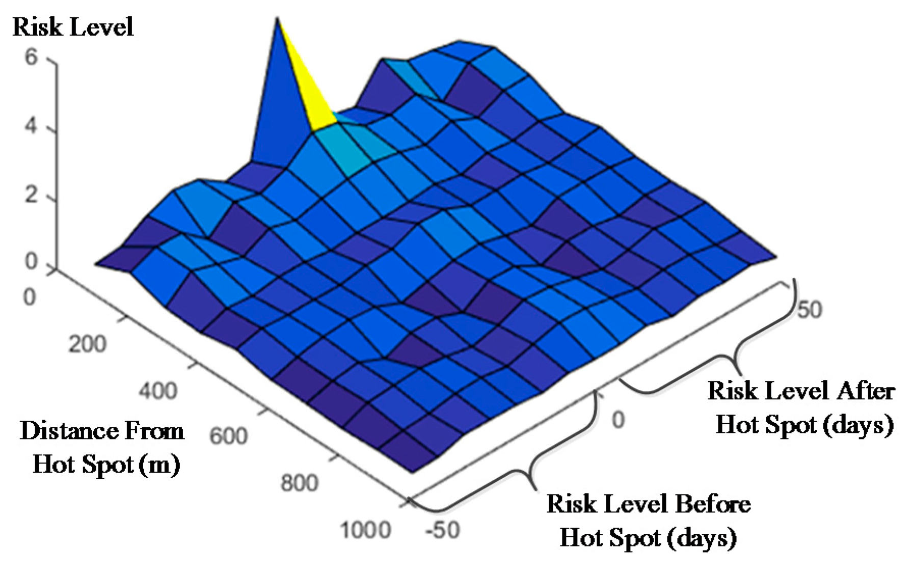
This section will analyze and quantify the crime risk level after the formation of hot spots based on the TENRM method. The experiments are performed on two different scales similar to the ‘hot spot contribution’ analysis. Two different scale matrices are obtained (Table 4 and Table 5), and two diagrams are given to analyze the undulation of the risk level around the hot spots (Figure 3 and Figure 4). The results on the two different scales are very similar. In general, a shorter space-time distance results in a higher risk level. This is also similar to the result of the ‘contribution matrix’ analysis.
In the result on the 100 m and seven day scale, the risk level within 200 m and seven days is nearly twice that of the normal level. The risk level near the hot spots will also increase simultaneously. For example, a risk level at day ‘0’ and ‘100–200’ m is 2.16 times higher than normal, which suggests an additional week with high crime risk following the hot spots. The risk level deceases as the distance gradually increases within the range of 400 m. However, the risk increases again in the day ‘0’ and ‘400–900’ meter bands. Thus, when a hot spot forms, another high risk location may exist nearby (400–900 m). This phenomenon suggests that different locales may be characterized by high crime risks simultaneously. Before the occurrence of hot spots, the crime risk levels of several adjacent units did not increase significantly. For example, the risk level of the two bands within ‘200’ m and ‘0–7’ days did not increase significantly, although the bands around them have a relatively high risk level (‘<100’ and ‘−15–21’, ‘100–300’ and ‘0–21’). It appears then that hot spot locations occur abruptly coincident with many crime incidents relative to normal conditions. However, the other bands near these bands also have high risk levels. Therefore, it appears that the hot spots move in space and time. This phenomenon has been discussed by Nakaya [33]. Moreover, the risk level rises significantly from ‘22’ to ‘42’ following hot spots, suggesting that hot spots will move to neighboring locations (i.e. within 100–300 m) and return to former sites three to five weeks later. As observed from the image view of the TENRM (Figure 2), the transfer and reduction process of the crime risk level is wave-like in nature. In addition, the risk level within 400–800 m increases synchronous with the hot spot, and it continues for one week after the hot spot forms. Thus, to improve the accuracy of crime prediction, it is important to understand that hot spots may occur abruptly, move to adjacent locales, occur simultaneously, and subsequently return to their original location. These characteristics are all very important for crime researchers and investigators.
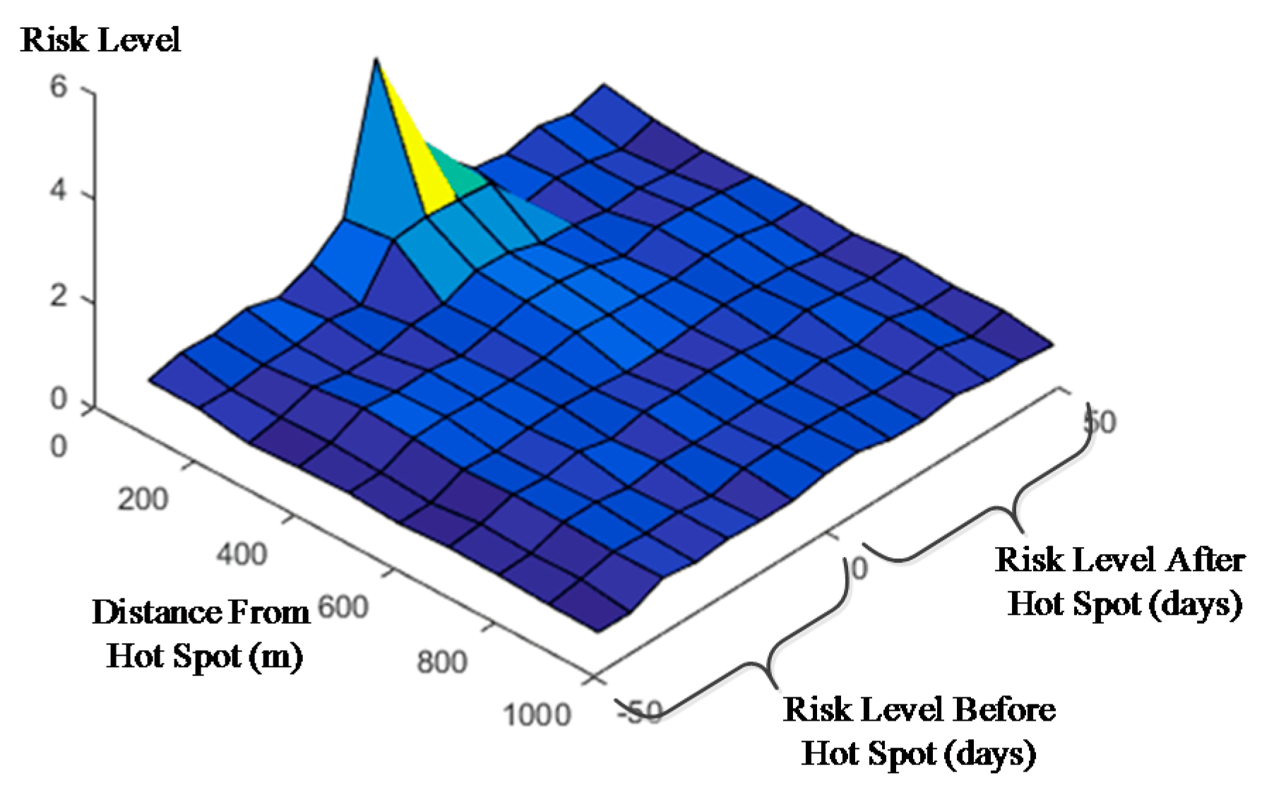
In the results for the 200 m and 14 day scale, the effects of the hot spot become weak with increasing space-time distance. This is similar to Table 1 and Table 4. The risk level seven days after the hot spot is 2.66 times higher than normal. In the period from seven days before and 14 days after a hot spot forms, the cells within a range of 500 m all have a higher risk level than normal. This may be caused by the change in the spatio-temporal scale. On a 200 m and 14 day scale, the range of the hot spots increases and more space-time bands are affected. In the bands following hot spot formation (15–35 days, 100–300 m), the risk level becomes very low, and the risk level at higher ranges (15–35 days, 300–500 m) becomes very high. This is similar to Figure 4 inasmuch as crime hot spots move in space and time. The risk level prior to a hot spot is not significant (−15–21, <100), but the nearby bands (−15–21 day, 100–200 m) occur within certain high-risk areas. Therefore, before hot spots are formed, the nearby area (100–300 m) always presents a high risk instead of the original location (<100 m). Beyond that, areas located from 600 m to 700 m from the hot spots also show a high risk. This pattern is similar to that of the band in the aforementioned case in that the risk level also shows a wavy undulation (Figure 4). As observed from the experimental results on the 200 m-14 day scale, the patterns before and after hot spots are roughly similar.
6. Discussion
The experiment conducted in this paper proves that in a large city in southeastern China, there exists near-repeat victimization in burglary scenarios. This is consistent with previous research results in other large American [28] and Chinese cities [32,38]. Currently, most research is focused on how much near repeats are involved in hot spots and how to use the theories concerning near-repeat victimization to interpret the formation of hot spots. In other words, numerous research studies have focused on the internal mechanisms of hot spots. Minimal research has investigated the risk outside (before and after) hot spots. The research concerning near-repeat victimization treats all crime events as having the same ability to ‘burst’ or induce future crime incidents [38].
In this paper, we investigated the relationship between hot spots and near-repeat victimization on two different space-time scales. The experiment on the scale of 100 m and seven days shows that hot spots provide a larger contribution to the increased risk level within 300 m and 21 days. Meanwhile, an experiment on another scale shows that hot spots also contribute substantially to near repeats within 1000 m and 42 days. These results show that hot spots contribute, in large measure, to near-repeat victimization on different space-time scales (Figure 2 and Figure 3). Therefore, hot-spot-related victimizations are different from other types inasmuch as they ‘burst’ future criminal victimizations. This conclusion not only sufficiently certifies the relationship between hot spots and near-repeat victimization but also poses the question of how to quantify the risk level before and after hot spots.
The temporal expanded near repeat matrix (TENRM) was proposed to analyze the risk level before and after hot spots. The experiments were processed on two space-time scales. Although the results on two space-time scales show some differences, they generally remain similar. First, the crime risk level decreases with increasing space and time distance after the formation of a hot spot. This pattern is similar to near repeats.
Second, crime risk moves in space and time. The risk level remains low before hot spots form, and the risk lasts for a certain amount of time afterward. However, the adjacent areas before and after hot spots are characterized by a high crime risk. This phenomenon can be interpreted by offender foraging explanations [19]. The active offenders in a hot spot may acquire more knowledge of nearby areas. The experienced offenders might become sensitive to new opportunities, which leads to a high risk level within the nearby areas. Specifically, before and after crime hot spots form, the crime risk level moves in space and time. Current research mostly considers repeat and near-repeat victimizations as the main components of hot spots. Many theories have also been proposed to interpret the formation of hot spots. In this paper, we analyze the risk displacement outside hot spots rather than the internal formation of hot spots. Existing research on crime displacement interprets the phenomenon to be a result of interactions with local policing activities. It is also interpreted that offenders always change to another attractive target considering the enhanced crime-prevention activities after the outbreak of hot spots [35,36]. In general, crime risk levels are characterized by a wave-like reduction process. This conclusion is useful in crime prediction and police patrols.
Third, simultaneous with the formation of hot spots, some high risk areas may exist nearby. This phenomenon may be caused by the periodic nature of burglaries. For example, studies show that the occurrence of crimes follows a certain pattern on a daily basis [50]. Other studies also demonstrate crime patterns both monthly and seasonally [51]. The difference here is that the result in this paper is processed on another scale.
7. Conclusions
We have described a new approach for crime risk investigation after proposing a method called the temporal expanded near-repeat matrix. Existing research on crime risk investigation is mainly based on repeat and near-repeat victimizations, which consider the risk level after every crime event. Compared to traditional analysis, this new method using a hot spot as the initial cell is particularly useful after considering the information over a past period as well as in quantifying the diffusion and displacement of crime risk.
Our model is designed to use a hot spot detection method and the Knox method for crime risk measurements. We choose a grid-based hot spot detection method to place hot spots into the matrix in the Knox method. To investigate the risk prior to the occurrence of a hot spot, the temporal axis is expanded in the matrix. The bandwidth is unified to be 100 m and seven days. Based on this matrix, the risk level pattern before and after hot spot occurrence is analyzed.
The conclusions herein are based on data from the large Chinese city of N. First, the current study investigates the existence of the near-repeat phenomenon from the literature using burglary data from N, China. The risk level shortly after every crime event will rise sharply but then decrease slowly. This is consistent with previous studies. Second, through a post-experiment analysis, it is proven that crime hot spots provide additional contributions to the near-repeat phenomena. Finally, a temporal expanded near repeat matrix (TENRM) was proposed to combine hot spots and the near-repeat phenomena. The experimental results show that crime hot spots always occur abruptly and disappear slowly. Furthermore, crime risk always moves in space and time. Thus, when a high risk forms near a given location, it can generate a hot spot. After the hot spot forms, the risk level may move to another area nearby. The distance depends on the hot spot scale. Another, more interesting fact is that hot spots may return after several days. An interpretation about crime displacement is also discussed. The conclusions in this study can be used to facilitate a detailed analysis of crime patterns, which not only advances previous research but also provides valuable results for crime prediction and prevention.
Certainly, there are limitations worth noticing in this study. The first limitation is related to the crime data that we relied on. Due to the format of the crime data, it is difficult to recognize crime pairs with the same location. Thus, repeat and near-repeat victimizations are not distinguished in this study. The second limitation is that the model has only been tested using crime data from a city in China. A comparison experiment with other areas is needed for future studies. The third limitation is that the analysis assumes a continuous space over which offenders can operate. The analysis cannot be performed where houses are present. Thus, how the availability of housing within the model impacts burglaries will be discussed in future studies.
Acknowledgments
This work was supported by the National Natural Science Foundation of China (No. 41501488), Surveying and Mapping Geographic Information Scientific Research Project in Jiangsu Province (No. JSCHKY201602), Youth Science and Technology Innovation Fund of Nanjing Forestry University (No. CX2015007), and the Open Research Fund Program of Key Laboratory of Police Geographic Information Technology, Ministry of Public Security (No. 2016 LPGIT06).
Author Contributions
Zengli Wang designed the research and analyzed the data; Xuejun Liu provided feedback on analysis and edited the paper.
Conflicts of Interest
The authors declare no conflict of interest.
References
- Johnson, S.D.; Bowers, K.J. The burglary as clue to the future: The beginnings of prospective hot-spotting. Eur. J. Criminol. 2004, 1, 237–255. [Google Scholar] [CrossRef]
- Townsley, M.; Homel, R.; Chaseling, J. Repeat burglary victimization: Spatial and temporal patterns. Aust. N. Z. J. Criminol. 2000, 33, 37–63. [Google Scholar] [CrossRef]
- Jochelson, R. Crime and Place: An Analysis of Assaults and Robberies in Inner Sydney; General Report Series; New SouthWales Bureau of Crime Statistics and Research: Sydney, Australia, 1997.
- Ratcliffe, J.H.; Rengert, G.F. Near-repeat patterns in Philadelphia shootings. Secur. J. 2008, 21, 58–76. [Google Scholar] [CrossRef]
- Shaw, C.R.; McKay, H.D. Social Factors in Juvenile Delinquency; Government Press: New York, NY, USA, 1931.
- Quetelet, A.J. Sur l’Homme et le Développement de ses Facultés, ou Essai de Physique Sociale; Bachelier: Paris, France, 1835. [Google Scholar]
- Mastrofski, S.D.; Weisburd, D.; Braga, A.A. Rethinking policing: The policy implications of hot spots of crime. In Contemporary Issues in Criminal Justice Policy, 2010Belmont; Natasha, F., Joshua, F., Todd, C., Eds.; CAWadsworth Cengage Learning: Boston, MA, USA, 2010; pp. 251–264. [Google Scholar]
- Cohen, L.E.; Felson, M. Social change and crime rate trends: A routine activity approach. Am. Sociol. Rev. 1979, 44, 588–608. [Google Scholar] [CrossRef]
- Clarke, R.V.G. Situational Crime Prevention: Successful Case Studies; Criminal Justice Press: Cincinnati, OH, USA, 1997. [Google Scholar]
- Rengert, G.F. The Journey to Crime: Conceptual Foundations and Policy Implications; Crime Policing Place: Essays in Environmental Criminology; Routledge: London, UK, 1992; pp. 109–117. [Google Scholar]
- Brantingham, P.L.; Brantingham, P.J. Crime pattern theory. In Environmental Criminology and Crime Analysis; Wortley, R., Mazerolle, L., Rombouts, S., Eds.; Willan Publishing: Cullompton, UK, 2008; pp. 78–93. [Google Scholar]
- Pease, K. Repeat Victimization: Taking Stock; Police Research Group: Crime Detection and Prevention Series Paper 90; The Home Office: London, UK, 1998.
- Morgan, F. Repeat burglary in a Perth suburb: Indicator of short-term or long-term risk? In Repeat Victimization; Farrell, G., Pease, K., Eds.; Monsey: New York, NY, USA, 2001; pp. 83–118. [Google Scholar]
- Johnson, S.D. Repeat burglary victimisation: A tale of two theories. J. Exp. Criminol. 2008, 4, 215–240. [Google Scholar] [CrossRef]
- Farrell, G.; Phillips, C.; Pease, K. Like taking candy: Why does repeat victimization occur? Br. J. Criminol. 1995, 35, 384–399. [Google Scholar] [CrossRef]
- Helbich, M.; Leitner, M. Frontiers in Spatial and Spatiotemporal Crime Analytics—An Editorial. ISPRS Int. J. Geo-Inf. 2017, 6, 73. [Google Scholar] [CrossRef]
- Sagovsky, A.; Johnson, S.D. When does repeat burglary occur? Aust. N. Z. J. Criminol. 2007, 40, 1–26. [Google Scholar] [CrossRef]
- Bowers, K.J.; Johnson, S.D. Who commits near repeats? A test of the boost explanation. Western Criminol. Rev. 2004, 5, 12–24. [Google Scholar]
- Johnson, S.D.; Summers, L.; Pease, K. Offender as forager? A direct test of the boost account of victimization. J. Quant. Criminol. 2009, 25, 181–200. [Google Scholar] [CrossRef]
- Knox, E.G.; Bartlett, M.S. The detection of space-time interactions. J. R. Stat. Soc. Series C (Appl. Stat.) 1964, 13, 25–30. [Google Scholar] [CrossRef]
- Townsley, M.; Homel, R.; Chaseling, J. Infectious burglaries: A test of the near repeat hypothesis. Br. J. Criminol. 2003, 43, 615–633. [Google Scholar] [CrossRef]
- Johnson, S.D.; Bernasco, W.; Bowers, K.J.; Elffers, H.; Ratcliffe, J.; Rengert, G.; Townsley, M. Space–time patterns of risk: A cross national assessment of residential burglary victimization. J. Quant. Criminol. 2007, 23, 201–219. [Google Scholar] [CrossRef]
- Johnson, S.D.; Bowers, K.J.; Birks, D.J.; Pease, K. Predictive mapping of crime by ProMap: Accuracy, units of analysis, and the environmental backcloth. In Putting Crime in Its Place; Springer: New York, NY, USA, 2009; pp. 171–198. [Google Scholar]
- Short, M.B.; D’Orsogna, M.R.; Brantingham, P.J.; Tita, G.E. Measuring and modeling repeat and near-repeat burglary effects. J. Quant. Criminol. 2009, 25, 325–339. [Google Scholar] [CrossRef]
- Bowers, K.J.; Johnson, S.D.; Pease, K. Prospective hot-spotting the future of crime mapping? Br. J. Criminol. 2004, 44, 641–658. [Google Scholar] [CrossRef]
- Johnson, S.D.; Birks, D.J.; McLaughlin, L.; Bowers, K.J.; Pease, K. Prospective Crime Mapping in Operational Context: Final Report; UCL, Jill Dando Institute of Crime Science: London, UK, 2007. [Google Scholar]
- Block, C.R. STAC hot-spot areas: A statistical tool for law enforcement decisions. In Crime Analysis Through Computer Mapping; Police Executive Research Forum: Washington, DC, USA, 1995; pp. 15–32. [Google Scholar]
- Ratcliffe, J.H.; McCullagh, M.J. Identifying repeat victimization with GIS. Br. J. Criminol. 1998, 38, 651–662. [Google Scholar] [CrossRef]
- Brunsdon, C.; Corcoran, J.; Higgs, G. Visualising space and time in crime patterns: A comparison of methods. Comput. Environ. Urban Syst. 2007, 31, 52–75. [Google Scholar] [CrossRef]
- Shiode, S.; Shiode, N. Network-based space-time search-window technique for hotspot detection of street-level crime incidents. Int. J. Geogr. Inf. Sci. 2013, 27, 866–882. [Google Scholar] [CrossRef]
- Haberman, C.P.; Ratcliffe, J.H. The predictive policing challenges of near repeat armed street robberies. Policing 2012, 6, 151–166. [Google Scholar] [CrossRef]
- Wu, L.; Xu, X.; Ye, X.; Zhu, X. Repeat and near-repeat burglaries and offender involvement in a large Chinese city. Cartogr. Geogr. Inf. Sci. 2015, 42, 178–189. [Google Scholar] [CrossRef]
- Nakaya, T.; Yano, K. Visualising crime clusters in a space-time cube: An exploratory data-analysis approach using space-time kernel density estimation and scan statistics. Trans. GIS 2010, 14, 223–239. [Google Scholar] [CrossRef]
- Leong, K.; Li, J.; Chan, S.C.; Ng, V. An application of the dynamic pattern analysis framework to the analysis of spatial-temporal crime relationships. J. UCS 2009, 15, 1852–1870. [Google Scholar]
- Piquero, A.R. Rational Choice and Criminal Behavior: Recent Research and Future Challenges; Routledge: London, UK, 2012. [Google Scholar]
- Paulsen, D.J.; Robinson, M.B. Spatial Aspects of Crime: Theory and Practice; Allyn & Bacon: Boston, MA, USA, 2004. [Google Scholar]
- Groff, E.R.; Johnson, L.; Ratcliffe, J.H.; Wood, J. Exploring the relationship between foot and car patrol in violent crime areas. Policing 2013, 36, 119–139. [Google Scholar] [CrossRef]
- Chen, P.; Yuan, H.; Li, D. Space-time analysis of burglary in Beijing. Secur. J. 2013, 26, 1–15. [Google Scholar] [CrossRef]
- Wang, Z.; Liu, X.; Lu, J. Multiscale geographic analysis of burglary. ACTA Geogr. Sin. 2017, 72, 329–340. [Google Scholar]
- Xu, C.; Zhou, S.; Liu, L. Patterns of near-repeat street robbery in DP peninsula. Geogr. Res. 2015, 34, 384–394. [Google Scholar]
- Wang, Z.; Liu, X.; Wu, W.; Lu, J. Construction and spatial-temporal analysis of crime network: A case study on burglary. Geomatics and Information Science of Wuhan University. Available online: http://www.cnki.net/kcms/detail/42.1676.TN.20160714.1324.003.html (accessed on 9 May 2017).
- Ratcliffe, J.H.; McCullagh, M.J. Hotbeds of crime and the search for spatial accuracy. J. Geogr. Syst. 1999, 1, 385–398. [Google Scholar] [CrossRef]
- McLafferty, S.; Williamson, D.; McGuire, P.G. Identifying crime hot spots using kernel smoothing. In Analyzing Crime Patterns: Frontiers of Practice; SAGE Publications: Thousand Oaks, CA, USA, 2000; pp. 77–85. [Google Scholar]
- Block, R.L.; Block, C.R. Space, place and crime: Hot spot areas and hot places of liquor-related crime. Crime Place 1995, 4, 145–184. [Google Scholar]
- Levine, N. CrimeStat III: A Spatial Statistics Program for the Analysis of Crime Incident Locations (version 3.0); Ned Levine & Associates: Houston, TX, USA; National Institute of Justice: Washington, DC, USA, 2004.
- Duczmal, L.; Assuncao, R. A simulated annealing strategy for the detection of arbitrarily shaped spatial clusters. Comput. Stat. Data Anal. 2004, 45, 269–286. [Google Scholar] [CrossRef]
- Takahashi, K.; Kulldorff, M.; Tango, T.; Yih, K. A flexibly shaped space-time scan statistic for disease outbreak detection and monitoring. Int. J. Health Geogr. 2008, 7, 14. [Google Scholar] [CrossRef] [PubMed]
- Shiode, S. Street-level spatial scan statistic and STAC for analysing street crime concentrations. Trans. GIS 2011, 15, 365–383. [Google Scholar] [CrossRef]
- Glasner, P.; Leitner, M. Evaluating the Impact the Weekday Has on Near-Repeat Victimization: A Spatio-Temporal Analysis of Street Robberies in the City of Vienna, Austria. ISPRS Int. J. Geo-Inf. 2016, 6, 3. [Google Scholar] [CrossRef]
- Chen, P.; Shu, X.; Yan, J.; Yuan, H. Timing of criminal activities during the day. J. Tsinghua Univ. (Sci. Tech.) 2009, 49, 2036–2039. [Google Scholar]
- Andresen, M.A.; Malleson, N. Crime seasonality and its variations across space. Appl. Geogr. 2013, 43, 25–35. [Google Scholar] [CrossRef]
Figure 1.
Overview of the study area.

Figure 2.
Diagram of temporal expanded near-repeat algorithm.

Figure 3.
Image from TENRM of hot spots (100 m and seven days).

Figure 4.
Image from TENRM of hot spots (200 m and 14 days).


Table 1.
Near-repeat results of the research area.
| Spatial Distance (m) | Temporal Distance (Day) | ||||||
|---|---|---|---|---|---|---|---|
| 0–7 | 8–14 | 15–21 | 22–28 | 29–35 | 35–42 | 42+ | |
| <100 | 2.85 ** | 1.77 ** | 1.70 ** | 1.72 ** | 1.45 ** | 1.29 ** | 1.05 |
| 100–200 | 1.81 ** | 1.50 ** | 1.41 ** | 1.32 ** | 1.15 ** | 1.02 | 1.02 |
| 200–300 | 1.72 ** | 1.54 ** | 1.37 ** | 1.34 ** | 1.20 ** | 1.09 | 1.09 |
| 300–400 | 1.48 ** | 1.35 ** | 1.28 ** | 1.26 ** | 1.19 ** | 1.11 * | 1.04 |
| 400–500 | 1.43 ** | 1.37 ** | 1.29 ** | 1.23 ** | 1.18 ** | 1.15 * | 1.12 |
| 500–600 | 1.28 ** | 1.28 ** | 1.19 ** | 1.17 * | 1.16 * | 1.16 * | 1.05 |
| 600–700 | 1.27 ** | 1.21 ** | 1.19 ** | 1.10 * | 1.05 | 1.03 | 1.01 |
| 700–800 | 1.24 ** | 1.20 ** | 1.12 * | 1.09 | 1.04 | 1.05 | 1.01 |
| 800–900 | 1.27 * | 1.19 * | 1.16 * | 1.11 * | 1.08 | 1.03 | 1.08 |
| 900–1000 | 1.20 * | 1.15 * | 1.08 | 1.13 * | 1.10 | 1.13 | 1.06 |
Note: * p < 0.01, ** p < 0.001.
Table 2.
Contributions of hot spots to near-repeat phenomena (100 m and seven days).
| Spatial Distance (m) | Temporal Distance (Day) | ||||||
|---|---|---|---|---|---|---|---|
| 0–7 | 8–14 | 15–21 | 22–28 | 29–35 | 35–42 | 42+ | |
| <100 | 62.2% | 34.7% | 33.9% | 29.5% | 28.9% | 27.5% | 26.6% |
| 100–200 | 37.0% | 30.3% | 26.1% | 26.2% | 26.3% | 27.3% | 26.6% |
| 200–300 | 29.2% | 28.2% | 26.1% | 25.5% | 24.4% | 26.2% | 22.6% |
| 300–400 | 25.8% | 24.9% | 24.6% | 25.6% | 24.4% | 25.4% | 24.8% |
| 400–500 | 26.9% | 23.4% | 24.4% | 22.7% | 25.6% | 26.4% | 22.6% |
| 500–600 | 26.5% | 25.5% | 24.7% | 24.0% | 24.3% | 24.4% | 25.1% |
| 600–700 | 25.3% | 23.9% | 25.4% | 24.2% | 24.3% | 23.6% | 24.0% |
| 700–800 | 25.4% | 24.4% | 25.2% | 25.0% | 24.2% | 24.7% | 23.5% |
| 800–900 | 25.7% | 24.9% | 24.2% | 24.1% | 25.4% | 24.6% | 24.1% |
| 900–1000 | 25.7% | 25.6% | 25.2% | 25.5% | 24.2% | 25.6% | 23.9% |
Table 3.
Contributions of hot spots to near-repeat phenomena (200 m and 14 days).
| Spatial Distance (m) | Temporal Distance (Day) | ||||||
|---|---|---|---|---|---|---|---|
| 0–7 | 8–14 | 15–21 | 22–28 | 29–35 | 35–42 | 42+ | |
| <100 | 100.0% | 98.5% | 79.3% | 72.0% | 70.6% | 64.2% | 61.1% |
| 100–200 | 100.0% | 99.3% | 78.7% | 71.5% | 71.9% | 65.7% | 60.1% |
| 200–300 | 74.9% | 74.4% | 74.9% | 64.1% | 62.4% | 56.4% | 53.8% |
| 300–400 | 71.4% | 70.7% | 68.3% | 61.5% | 60.2% | 54.5% | 49.8% |
| 400–500 | 66.3% | 66.8% | 65.9% | 58.3% | 57.6% | 51.3% | 46.0% |
| 500–600 | 64.2% | 64.8% | 63.1% | 55.0% | 56.3% | 46.5% | 45.0% |
| 600–700 | 63.9% | 60.7% | 60.9% | 52.5% | 49.8% | 44.8% | 41.3% |
| 700–800 | 57.0% | 58.4% | 57.7% | 50.0% | 47.5% | 38.1% | 38.0% |
| 800–900 | 55.7% | 57.6% | 54.5% | 50.0% | 46.8% | 41.9% | 37.8% |
| 900–1000 | 58.9% | 56.5% | 58.9% | 49.7% | 47.7% | 41.5% | 38.1% |
Table 4.
Temporal expanded near repeat matrix (TENRM) of hot spots (100 m and seven days)
| Temporal Distance (Day) | Spatial Distance (m) | |||||||||
|---|---|---|---|---|---|---|---|---|---|---|
| <100 | 100–200 | 200–300 | 300–400 | 400–500 | 500–600 | 600–700 | 700–800 | 800–900 | 900–1000 | |
| −43–49 | 0.78 | 1.21 ** | 0.86 | 0.80 | 1.00 | 0.78 | 0.77 | 0.72 | 0.77 | 0.77 |
| −36–42 | 0.85 | 1.52 ** | 1.49 ** | 1.08 | 1.17 * | 1.01 | 0.98 | 1.03 | 0.89 | 0.79 |
| −29–35 | 1.30 ** | 1.47 ** | 1.24 ** | 0.98 | 1.11 * | 1.15 * | 1.08 | 1.08 | 0.94 | 1.00 |
| −22–28 | 1.60 ** | 0.84 | 1.00 | 1.09 | 1.11 * | 1.20 * | 0.74 | 1.13 | 1.07 | 0.99 |
| −15–21 | 1.46 ** | 1.49 ** | 1.38 ** | 1.08 | 1.07 | 1.12 | 1.04 | 1.03 | 1.09 | 0.97 |
| −8–14 | 0.93 | 1.27 ** | 1.17 | 0.97 | 1.21 * | 0.79 | 1.05 | 0.86 | 0.97 | 0.87 |
| 0–7 | 1.09 | 1.56 ** | 1.35 ** | 1.03 | 1.23 * | 0.97 | 0.74 | 1.04 | 1.16 | 1.00 |
| 0 | 4.84 ** | 2.16 ** | 1.47 ** | 1.02 | 1.53 ** | 1.13 * | 1.22 * | 1.34 * | 1.35 * | 0.94 |
| 0–7 | 2.06 ** | 2.00 ** | 1.51 ** | 1.05 | 1.50 ** | 1.17 * | 1.19 * | 1.26 * | 1.32 * | 0.94 |
| 8–14 | 1.06 | 1.45 ** | 1.37 * | 1.11 * | 1.16 * | 0.95 | 0.76 | 1.07 | 1.16 | 1.04 |
| 15–21 | 0.88 | 1.32 ** | 1.13 * | 0.93 | 1.15 | 0.80 | 1.02 | 0.88 | 0.99 | 0.85 |
| 22–28 | 1.84 ** | 1.49 ** | 1.37 * | 1.13 * | 1.18 * | 1.18 * | 1.01 | 0.99 | 1.09 | 0.98 |
| 29–35 | 1.33 ** | 0.80 | 1.01 | 1.03 | 1.05 | 1.17 | 0.86 | 1.16 | 1.08 | 0.95 |
| 36–42 | 1.20 ** | 1.50 ** | 1.36 * | 1.14 * | 1.13 * | 1.14 * | 1.01 | 1.05 | 0.92 | 1.01 |
| 43–49 | 1.02 | 1.50 * | 1.37 * | 0.93 | 1.20 | 1.03 | 0.97 | 1.04 | 0.87 | 0.78 |
Note: * p < 0.01, ** p < 0.001.
Table 5.
TENRM of hot spots (200 m and 14 days).
| Temporal Distance (Day) | Spatial Distance (m) | |||||||||
|---|---|---|---|---|---|---|---|---|---|---|
| <100 | 100–200 | 200–300 | 300–400 | 400–500 | 500–600 | 600–700 | 700–800 | 800–900 | 900–1000 | |
| −43–49 | 0.98 | 0.97 | 0.81 | 0.87 | 0.90 | 0.83 | 0.89 | 0.87 | 0.82 | 0.80 |
| −36–42 | 1.13 * | 0.95 | 0.92 | 0.95 | 0.90 | 0.83 | 0.95 | 0.90 | 0.92 | 0.79 |
| −29–35 | 1.09 | 1.02 | 1.11 * | 1.23 * | 1.17 * | 1.08 | 1.12 | 1.11 | 1.06 | 1.08 |
| −22–28 | 1.20 * | 1.02 | 1.00 | 1.15 * | 1.18 * | 1.04 | 1.06 | 1.10 | 1.02 | 0.98 |
| −15–21 | 1.02 | 1.11 * | 0.99 | 1.17 * | 1.14 * | 1.10 * | 1.17 * | 1.00 | 1.04 | 1.04 |
| −8–14 | 1.27 * | 1.00 | 1.13 * | 1.06 | 1.11 | 1.12 | 1.01 | 1.09 | 0.95 | 1.00 |
| −0–7 | 1.75 ** | 1.86 ** | 1.15 * | 1.19 * | 1.15 * | 1.07 | 1.15 * | 1.06 | 1.10 | 1.00 |
| Hot spot | 4.44 ** | 1.91 ** | 1.40 * | 1.32 * | 1.25 * | 1.00 | 1.13 * | 1.06 | 1.12 | 1.13 |
| 0–7 | 2.66 ** | 1.85 ** | 1.36 * | 1.32 * | 1.20 * | 1.01 | 1.15 * | 1.08 | 1.11 | 1.16 |
| 8–14 | 1.77 ** | 1.78 ** | 1.15 * | 1.22 * | 1.15 * | 1.07 | 1.13 * | 1.05 | 1.08 | 1.01 |
| 15–21 | 1.16 * | 1.01 | 1.10 | 1.03 | 1.11 * | 1.13 * | 1.04 | 1.10 | 0.99 | 0.98 |
| 22–28 | 1.05 | 1.10 * | 0.99 | 1.19 * | 1.17 * | 1.09 | 1.16 * | 0.99 | 0.99 | 1.07 |
| 29–35 | 1.19 * | 1.03 | 1.03 | 1.15 * | 1.15 * | 1.05 | 1.07 | 1.12 * | 1.07 | 0.96 |
| 36-42 | 1.04 | 0.88 | 0.95 | 1.09 | 1.01 | 0.93 | 0.98 | 0.95 | 0.90 | 0.94 |
| 43-49 | 1.22 * | 1.06 | 0.98 | 1.00 | 1.00 | 0.93 | 1.02 | 0.96 | 1.01 | 0.87 |
Note: * p < 0.01, ** p < 0.001.
© 2017 by the authors. Licensee MDPI, Basel, Switzerland. This article is an open access article distributed under the terms and conditions of the Creative Commons Attribution (CC BY) license (http://creativecommons.org/licenses/by/4.0/).
Share and Cite
MDPI and ACS Style
Wang, Z.; Liu, X. Analysis of Burglary Hot Spots and Near-Repeat Victimization in a Large Chinese City. ISPRS Int. J. Geo-Inf. 2017, 6, 148. https://0-doi-org.brum.beds.ac.uk/10.3390/ijgi6050148
AMA Style
Wang Z, Liu X. Analysis of Burglary Hot Spots and Near-Repeat Victimization in a Large Chinese City. ISPRS International Journal of Geo-Information. 2017; 6(5):148. https://0-doi-org.brum.beds.ac.uk/10.3390/ijgi6050148
Chicago/Turabian StyleWang, Zengli, and Xuejun Liu. 2017. "Analysis of Burglary Hot Spots and Near-Repeat Victimization in a Large Chinese City" ISPRS International Journal of Geo-Information 6, no. 5: 148. https://0-doi-org.brum.beds.ac.uk/10.3390/ijgi6050148
Note that from the first issue of 2016, this journal uses article numbers instead of page numbers. See further details here.